Learning Green’s Functions of Linear Reaction-Diffusion Equations with Application to Fast Numerical Solver

Abstract

Partial differential equations are commonly used to model various physical phenomena, such as heat diffusion, wave propagation, fluid dynamics, elasticity, electrodynamics and so on. Due to their tremendous applications in scientific and engineering research, many numerical methods have been developed in past decades for efficient and accurate solutions of these equations on modern computing systems. Inspired by the rapidly growing impact of deep learning techniques, we propose in this paper a novel neural network method, “GF-Net”, for learning the Green’s functions of the classic linear reaction-diffusion equation with Dirichlet boundary condition in the unsupervised fashion. The proposed method overcomes the numerical challenges for finding the Green’s functions of the equations on general domains by utilizing the physics-informed neural network and the domain decomposition approach. As a consequence, it also leads to a fast numerical solver for the target equation subject to arbitrarily given sources and boundary values without network retraining. We numerically demonstrate the effectiveness of the proposed method by extensive experiments with various domains and operator coefficients.

1 Introduction

Rapid development and great success of deep learning for computer vision and natural language processing have significantly prompted its application to many other science and engineering problems in recent years. Thanks to the integration of available big data, effective learning algorithms and unprecedented computing powers, the resulted deep learning studies have showed increasing impacts on various subjects including partial differential equations (PDEs), dynamical system, reduced order modeling and so on. In particular, the synthesis of deep learning techniques and numerical solution of PDEs has become an emerging research topic in addition to conventional numerical methods such as finite difference, finite element and finite volume ones.

Some popular deep learning algorithms include the physics-informed neural networks (PINNs) (Raissi et al., 2019), the deep Ritz method (DRM) (E and Yu, 2018), the deep Galerkin method (DGM) (Sirignano and Spiliopoulos, 2018) and the PDE-Net (Long et al., 2018). Note that the first three are meshfree and trained without any explicitly observed data and the last one uses instead rectangular meshes and ground-truth information for training. Deep learning based methods also have been applied to construct computational surrogates for PDE models in a series of research (Khoo et al., 2021; Nagoor Kani and Elsheikh, 2017; Nabian and Meidani, 2019; Lee and Carlberg, 2020; San et al., 2019; Mücke et al., 2019; Zhu et al., 2019; Sun et al., 2020). On the other hand, classic methods for solving PDEs also have been used to understand and further improve the network structure and training settings. For instance, the connection between multigrid methods and convolutional neural networks (CNNs) was discussed in (He and Xu, 2019) and MGNet was then proposed to incorporate them.

The goal of our work is to design a neural network based method for fast numerical solution of the classic linear reaction-diffusion equation on arbitrary domains, that could yield an accurate response to various sources and Dirichlet boundary values without retraining. To achieve this, we propose a neural network, called “GF-Net”, that computes the Green’s functions associated with the target PDE under Dirichlet boundary conditions. Note that the exact solution of the target equation can be explicitly expressed in terms of the Green’s function, source term and boundary values via area and line integrals (Evans, 1998). After evaluating the Green’s function at a set of sample points with the trained GF-Net, the target PDE problem can numerically be solved in an efficient manner. As the Green’s function is the impulse response of the linear differential operator, which is well approximated by the GF-Net through a nonlinear mapping, a significant advantage of the proposed method compared to most existing deep learning methods for numerical PDEs is that it does not need network retraining when the PDE source and/or the Dirichlet boundary condition change. How to determine the Green’s functions of a PDE is a classic problem. The analytic formulation of Green’s functions are only known for a few operators on either open spaces or domains with simple geometry (Evans, 1998), such as the linear reaction-diffusion operator. On the other hand, finding their numerical approximations by traditional numerical methods often turns out to be too expensive in terms of computation and memory. In addition, the high-dimensional parameter space makes it almost impossible to use model reduction to find efficient surrogates for the Green’s functions.

In this paper, we propose a neural network architecture GF-Net that can provide a new way to tackle this classic problem for the linear reaction-diffusion equation with Dirichlet boundary condition through deep learning to overcome some limitations of traditional methods. In particular, our GF-Net is physics-informed: a forward neural network is trained by minimizing the loss function measuring the pointwise residuals, discrepancy in boundary values, and an additional term for penalizing the asymmetry of the output due to the underlying property of symmetry possessed by Green’s functions. Meanwhile, to accelerate the training process, we also design a sampling strategy based on the position of the point source, and further put forth a domain decomposition approach to train multiple GF-Nets in parallel on many blocks. Note that each GF-Net is assigned and associated with a specific subdomain block. Finally, the application of the produced GF-Nets to fast numerical solution of the target equation with different sources and boundary values is carefully tested and demonstrated through experiments with various domain and operator coefficients.

2 Related work

Using neural networks to solve differential equations has been investigated in several early works, e.g., (Dissanayake and Phan-Thien, 1994; Lagaris et al., 1998), and recent advances in deep learning techniques have further stimulated new exploration towards this direction.

The physics-informed neural network (PINN) (Raissi et al., 2019) represents the mapping from spatial and/or temporal variables to the state of the system by deep neural networks, which is then trained by minimizing the weighted sum of the residuals of PDEs at randomly selected interior points and the errors at initial/boundary points. This approach later has been extended to solve inverse problems (Raissi et al., 2020), fractional differential equations (Pang et al., 2019), stochastic differential equations and uncertainty quantification (Nabian and Meidani, 2019; Yang et al., 2020; Zhang et al., 2020, 2019). Improved sampling and training strategies have been considered in (Lu et al., 2021b; Anitescu et al., 2019; Zhao and Wright, 2021; Krishnapriyan et al., 2021). In order to solve topology optimization problems for inverse design, PINNs with hard constraints were also investigated in (Lu et al., 2021c). The deep Ritz method (DRM) (E and Yu, 2018) considers the variational form of PDEs, which combines the mini-batch stochastic gradient descent algorithms with numerical integration to optimize the network. Note that later the variational formulation was also considered in weak adversarial networks (Zang et al., 2020). The deep Galerkin method (DGM) (Sirignano and Spiliopoulos, 2018) merges the classic Galerkin method and machine learning, that is specially designed for solving a class of high-dimensional free boundary PDEs. The above three learning methods use no meshes as opposed to traditional numerical methods and are trained in the unsupervised fashion (i.e., without ground-truth data). The PDE-Net (Long et al., 2018) proposes a stack of networks ($\delta t$-blocks) to advance the PDE solutions over a multiple of time steps. It recognizes the equivalence between convolutional filters and differentiation operators in rectangular meshes under the supervised training with ground-truth data. This approach was further combined with a symbolic multilayer neural network for recovering PDE models in (Long et al., 2019).

Learning the operators can provide better capability and efficiency by solving a whole family of PDEs instead of a single fixed equation. The Fourier neural operator (FNO) (Li et al., 2021a) aims to parameterize the integral kernel in Fourier space and is able to generalize trained models to different spatial and time resolutions. The DeepONet (Lu et al., 2021a) extends the universal approximation theorem for operators in (Chen and Chen, 1995) to deep neural networks. It contains two subnetworks to encoder the input functions and its transformed location variable respectively and then uses the extended theorem to generate the target output. DeepONet has quite powerful generalization ability to handle diverse linear/nonlinear explicit and implicit operators. Error estimation for DeepONet was recently investigated in (Lanthaler et al., 2022). Physics-informed DeepONets proposed in (Wang et al., 2021) further reduces the requirement for data and achieves up to three order of magnitude faster inference time than convectional method. Learning operators by using graph neural networks (GNN) was first considered in (Anandkumar et al., 2020) and later improved in (Li et al., 2020). In (Li et al., 2021b), the physics-informed neural operator (PINO), which combines the operator learning and function approximation frameworks to achieve higher accuracy, was proposed. In addition, attention mechanism was further introduced in (Kissas et al., 2022) to solve the climate prediction problem.

There also exist a few works which compute or use Green’s functions to solve PDEs. The data-driven method recently proposed in (Boullé et al., 2022) applies rational neural network structure to train networks with generated excitation for approximating Green’s functions and the homogeneous solution separately. The PINN was recently used to solving some PDEs with point source in (Huang et al., 2021). For handling nonlinear boundary value problems, the DeepGreen in (Gin et al., 2021) first linearizes the nonlinear problems using a dual autoencoder architecture, then evaluates the Green’s function of the linear operator, and finally inversely transforms the linear solution to solve the nonlinear problem.

3 Linear Reaction-diffusion equations and Green’s functions

Let $\Omega\subset\mathbb{R}^{d}$ be a bounded domain, we consider the linear reaction-diffusion operator of the following form:

$$\begin{array}[]{rrl}{\cal L}(u)({\boldsymbol{x}})&:=&-\nabla\cdot(a({\boldsymbol{x}})\nabla u({\boldsymbol{x}}))+r({\boldsymbol{x}})u({\boldsymbol{x}}),\quad{\boldsymbol{x}}\in\Omega,\end{array}$$ (1)

where $a({\boldsymbol{x}})>0$ is the diffusion coefficient and $r({\boldsymbol{x}})\geq 0$ is the reaction coefficient. The corresponding linear reaction-diffusion problem with Dirichlet boundary condition then reads:

$$\left\{\begin{array}[]{rl}{\cal L}(u)({\boldsymbol{x}})=f({\boldsymbol{x}}),&\quad{\boldsymbol{x}}\in\Omega,\\ u({\boldsymbol{x}})=g({\boldsymbol{x}}),&\quad{\boldsymbol{x}}\in\partial\Omega,\end{array}\right.$$ (2)

where $f({\boldsymbol{x}})$ is the given source term and $g({\boldsymbol{x}})$ the boundary value. The Green’s function $G({\boldsymbol{x}},{\boldsymbol{\xi}})$ represents the impulse response of the PDE subject to homogeneous Dirichlet boundary condition, that is, for any impulse source point ${\boldsymbol{\xi}}\in\Omega$,

$$\left\{\begin{array}[]{rl}{\cal L}(G)({\boldsymbol{x}},{\boldsymbol{\xi}})=\delta({\boldsymbol{x}}-{\boldsymbol{\xi}}),&\quad{\boldsymbol{x}}\in\Omega,\\ G({\boldsymbol{x}},{\boldsymbol{\xi}})=0,&\quad{\boldsymbol{x}}\in\partial\Omega,\end{array}\right.$$ (3)

where $\delta({\boldsymbol{x}})$ denotes the Dirac delta source function satisfying $\delta({\boldsymbol{x}})=0$ if ${\boldsymbol{x}}\neq{\bf 0}$ and $\int_{\mathbb{R}^{d}}\delta({\boldsymbol{x}})\,d{\boldsymbol{x}}=1$. Note that the Green’s function $G$ is symmetric, i.e., $G({\boldsymbol{x}},{\boldsymbol{\xi}})=G({\boldsymbol{\xi}},{\boldsymbol{x}})$. If $G({\boldsymbol{x}},{\boldsymbol{\xi}})$ is known, the solution of the problem (2) can be readily expressed by the following formula:

$$u({\boldsymbol{x}})=\int_{\Omega}f({\boldsymbol{\xi}})G({\boldsymbol{x}},{\boldsymbol{\xi}})\,d{\boldsymbol{\xi}}-\int_{\partial\Omega}g({\boldsymbol{\xi}})a({\boldsymbol{\xi}})({\nabla_{{\boldsymbol{\xi}}}G}({\boldsymbol{x}},{\boldsymbol{\xi}})\cdot{\vec{\bf n}}_{{\boldsymbol{\xi}}})\,dS({\boldsymbol{\xi}}),\quad\forall\,{\boldsymbol{x}}\in\Omega,$$ (4)

where ${\vec{\bf n}}_{{\boldsymbol{\xi}}}$ denotes the unit outer normal vector on $\partial\Omega$. However, the above Green’s function (i.e., the solution of (3)) on a general domain usually does not have analytic form, and consequently we need to numerically approximate the Green’s function.

4 GF-Net: Learning Green’s functions

We will construct a deep feedforward network, GF-Net, to learn the Green’s function associated with the operator (1), and then use it to fast solve the problem (2) based on the formula (4). In order to represent the Green’s function obeying (3), we adopt the framework of PINNs (Raissi et al., 2019), a fully connected neural network, with slight modifications and accommodate the symmetric characteristic of Green’s function into the network structure. In this work, we take the two-dimensional problem for illustration and testing of the GF-Net considering computing and memory budgets, but the proposed method can be naturally generalized to higher dimensions.

4.1 Network architecture

The architecture of GF-Net for a 2D problem is shown in Figure 1.

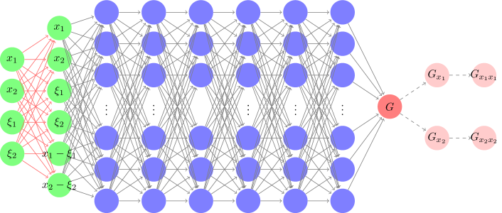
Figure 1: An illustration of the GF-Net architecture with 1 auxiliary layer (green) and 6 hidden layers (blue) for a 2D problem. The derivatives, such as $G_{x_{1}},G_{x_{1}x_{1}},\cdots$, can be naturally obtained by applying derivatives on $G$ with automatic differentiation.

The vector ${\boldsymbol{v}}=[{\boldsymbol{x}},{\boldsymbol{\xi}}]^{\intercal}$ is fed as input to the network, followed by an auxiliary layer without bias and activation:

$$\ell_{0}({\boldsymbol{x}},{\boldsymbol{\xi}})={\boldsymbol{W}}^{0}\left[\begin{array}[]{c}{\boldsymbol{x}}\\ {\boldsymbol{\xi}}\end{array}\right],~{}\quad{\boldsymbol{W}}^{0}=\left[\begin{array}[]{rr}{\boldsymbol{I}}&\boldsymbol{0}\\ \boldsymbol{0}&{\boldsymbol{I}}\\ {\boldsymbol{I}}&-{\boldsymbol{I}}\end{array}\right].$$

This is a preprocessing or auxiliary layer inspired by the formulation of the Greens’ function containing the variables ${\boldsymbol{x}},{\boldsymbol{\xi}}$ and ${\boldsymbol{x}}-{\boldsymbol{\xi}}$. The layer is then connected to $D-1$ hidden layers and an output layer, which form a fully-connected neural network of depth $D$. Letting $\ell_{k}$ be the $k$-th layer after the auxiliary layer, then this layer receives an input ${\boldsymbol{v}}^{k-1}$ from the previous layer output and transforms it by an affine mapping to

$$\ell_{k}({\boldsymbol{v}}^{k-1})={\boldsymbol{W}}^{k}{\boldsymbol{v}}^{k-1}+{\boldsymbol{b}}^{k},$$ (5)

where ${\boldsymbol{W}}^{k}$ is called the connection weight and ${\boldsymbol{b}}^{k}$ the bias. The nonlinear activation function $\sigma(\cdot)$ is applied to each component of the transformed vector before sending it to the next layer, except the last hidden one. The network thus is a composite of a sequence of nonlinear functions:

$$G({\boldsymbol{x}},{\boldsymbol{\xi}};{\boldsymbol{\Theta}})=\left(\ell_{D}\circ\sigma\circ\ell_{D-1}\circ\cdots\circ\sigma\circ\ell_{1}\circ\ell_{0}\right)({\boldsymbol{x}},{\boldsymbol{\xi}}),$$ (6)

where the operator “$\circ$” denotes the composition and ${\boldsymbol{\Theta}}=\{{\boldsymbol{W}}^{k},{\boldsymbol{b}}^{k}\}_{k=1}^{D}$ represents the trainable parameters in the network. It should be noted that the weight ${\boldsymbol{W}}^{0}$ is frozen that needs not to be updated during the training process.

4.2 Approximation of the Dirac delta function

In the network setting, we seek for a classic (smooth) solution satisfying the strong form of the PDE (3). However, $G({\boldsymbol{x}},{\boldsymbol{\xi}})$ is not differentiable everywhere as it is a response to the impulse source defined by the Dirac delta function. Indeed, it can only be well defined in the sense of distribution. In practice, we approximate the Dirac delta function by a multidimensional Gaussian density function:

$$\rho({\boldsymbol{x}}-{\boldsymbol{\xi}})={\frac{1}{(\sqrt{2\pi}s)^{2}}}e^{-\frac{|{\boldsymbol{x}}-{\boldsymbol{\xi}}|^{2}}{2s^{2}}},$$ (7)

where the parameter $s>0$ denotes the standard deviation of the distribution. As $s\rightarrow 0$, the function (7) converges to the Dirac delta function pointwisely except at the point ${\boldsymbol{x}}={\boldsymbol{\xi}}$.

4.3 Sampling strategy for the variable ${\boldsymbol{x}}$

Since the GF-Net takes both ${\boldsymbol{x}}$ and ${\boldsymbol{\xi}}$ as input, how to sample them in a reasonable manner could be crucial to the training process. In particular, the distribution of ${\boldsymbol{x}}$-samples with respect to different ${\boldsymbol{\xi}}$ should vary following the behaviour of $\rho({\boldsymbol{x}}-{\boldsymbol{\xi}})$: most samples need to be placed within $3$ standard deviations away from the mean of a Gaussian distribution based on the empirical rule.

To make the sampling effective, we put forth the following strategy: Since the spatial domain $\Omega$ may have complex geometrical shape, we adopt a mesh generator to first partition $\Omega$ into a triangular mesh $\mathcal{T}_{\boldsymbol{\xi}}=(\mathcal{V}_{\boldsymbol{\xi}},\mathcal{E}_{\boldsymbol{\xi}})$ where $\mathcal{V}_{\boldsymbol{\xi}}$ denotes the vertex set and $\mathcal{E}_{\boldsymbol{\xi}}$ denotes the edge set, and then collect ${\boldsymbol{\xi}}$-samples from the interior vertices to form $\mathcal{S}_{\boldsymbol{\xi}}=\{{\boldsymbol{\xi}}\in\mathcal{V}_{{\boldsymbol{\xi}}}:{\boldsymbol{\xi}}\notin\partial\Omega\}$. For each fixed ${\boldsymbol{\xi}}$, we select ${\boldsymbol{x}}$-samples that concentrate around it because the Gaussian density function centers at this ${\boldsymbol{\xi}}$. Hence, we generate another three meshes $\{\mathcal{T}_{\boldsymbol{x}}^{i}=(\mathcal{V}_{\boldsymbol{x}}^{i},\mathcal{E}_{\boldsymbol{x}}^{i})\}_{i=1}^{3}$ of resolutions from high to low, and collect ${\boldsymbol{x}}$-samples to form the set $\mathcal{S}_{{\boldsymbol{x}},{\boldsymbol{\xi}}}=\mathcal{S}_{{\boldsymbol{x}},{\boldsymbol{\xi}}}^{1}\cup\mathcal{S}_{{\boldsymbol{x}},{\boldsymbol{\xi}}}^{2}\cup\mathcal{S}_{{\boldsymbol{x}},{\boldsymbol{\xi}}}^{3},$ in which

$$\mathcal{S}_{{\boldsymbol{x}},{\boldsymbol{\xi}}}^{1} =\{{\boldsymbol{x}}\in\mathcal{V}_{\boldsymbol{x}}^{1}:\|{\boldsymbol{x}}-{\boldsymbol{\xi}}\|_{\infty}\leq c_{1}s\},$$

$$\mathcal{S}_{{\boldsymbol{x}},{\boldsymbol{\xi}}}^{2} =\{{\boldsymbol{x}}\in\mathcal{V}_{\boldsymbol{x}}^{2}:c_{1}s<\|{\boldsymbol{x}}-{\boldsymbol{\xi}}\|_{\infty}<c_{2}s\},$$

$$\mathcal{S}_{{\boldsymbol{x}},{\boldsymbol{\xi}}}^{3} =\{{\boldsymbol{x}}\in\mathcal{V}_{\boldsymbol{x}}^{3}:\|{\boldsymbol{x}}-{\boldsymbol{\xi}}\|_{\infty}\geq c_{2}s\},$$

and $c_{1},c_{2}$ are two hyperparameters. Finally, the overall dataset is selected as $\mathcal{S}=\{({\boldsymbol{x}},{\boldsymbol{\xi}}):{\boldsymbol{\xi}}\in\mathcal{S}_{\boldsymbol{\xi}},{\boldsymbol{x}}\in\mathcal{S}_{{\boldsymbol{x}},{\boldsymbol{\xi}}}\}.$ To highlight this sampling strategy, we plot in Figure 2 the ${\boldsymbol{x}}$-samples associated to given ${\boldsymbol{\xi}}$ in three types of domains (square, annulus and L-shaped) considered in numerical tests.

In all experiments, we adopt the mesh generator in (Ju, 2007) to generate the sampling points since it is easily applicable to plenty of commonly used complex domains. Random or pseudo-random sampling methods may have some inconveniences and need extra process in dealing with irregular regions; for instance, the popular Latin hypercube sampling (McKay et al., 1979) method plus the rejection procedure (Ross, 1976) also can be used here.

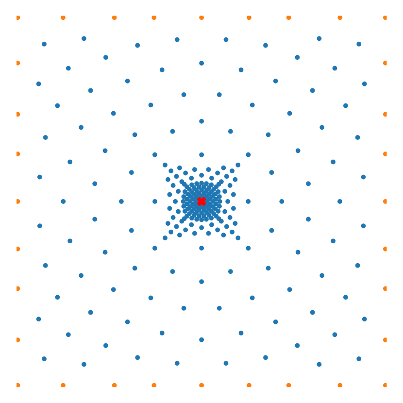
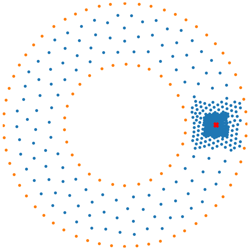
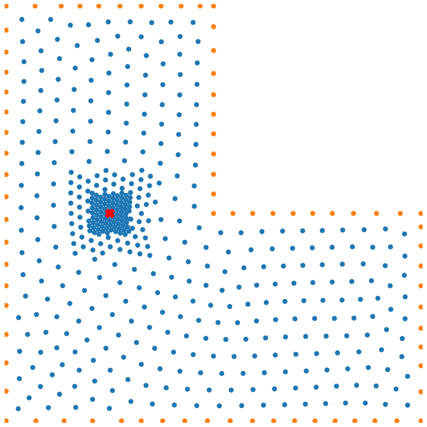
Figure 2: Locally refined ${\boldsymbol{x}}$-samples for a given ${\boldsymbol{\xi}}$ (marked by the large red cross). Left: ${\boldsymbol{\xi}}=(0,0)$ in a square; middle: ${\boldsymbol{\xi}}=(\frac{3}{4},0)$ in an annulus; right: ${\boldsymbol{\xi}}=(-\frac{1}{2},0)$ in a L-shaped domain.

4.4 Partitioning strategy for the point source location ${\boldsymbol{\xi}}$

Ideally, we wish to use one single GF-Net to model the Green’s function associated to any ${\boldsymbol{\xi}}$ in the domain $\Omega$, but such a network may easily become unmanageable due to a large amount of data in $\mathcal{S}$, or be very difficult to train as different ${\boldsymbol{\xi}}$ may yield totally distinct behaviors of the Green’s function. On the other hand, since the Green’s function corresponding to different ${\boldsymbol{\xi}}$ can be solved individually, it is feasible to train a GF-Net for each sample ${\boldsymbol{\xi}}$, which however would cause the loss of efficiency and result in large storage issues. Therefore, we propose an domain decomposition strategy for ${\boldsymbol{\xi}}$ and train a set of GF-Nets on ${\boldsymbol{\xi}}$-blocks. Given any target 2D domain $\Omega$, we first identify an circumscribed rectangle of $\Omega$, then divide it into $m\times n$ blocks uniformly. Suppose there are $K$ $(\leq m\times n)$ blocks containing samples of ${\boldsymbol{\xi}}$, we denote the ${\boldsymbol{\xi}}$-sample set in the $k$-th block by $\mathcal{S}_{{\boldsymbol{\xi}}}^{k}$, for $k=1,\ldots,K$. Figure 3 shows the ${\boldsymbol{\xi}}$-blocks associated to the three different domains (square, annulus and L-shaped). Consequently, we define the sample set associated to the $k$-th ${\boldsymbol{\xi}}$-block by $\mathcal{S}^{k}=\{({\boldsymbol{x}},{\boldsymbol{\xi}}):{\boldsymbol{\xi}}\in\mathcal{S}_{\boldsymbol{\xi}}^{k},{\boldsymbol{x}}\in\mathcal{S}_{{\boldsymbol{x}},{\boldsymbol{\xi}}}\}$. Based on the new partitioned samples, a set of $K$ GF-Nets will be independently trained. The approach has at least two advantages: first, the training tasks are divided into many small subtasks, which are naturally parallelizable and can be distributed to multiple GPUs for efficient implementations; second, locally trained models tend to obtain better accuracy and stronger generalization ability (for unseen/predicted ${\boldsymbol{\xi}}$ located in corresponding blocks) than the global single model.

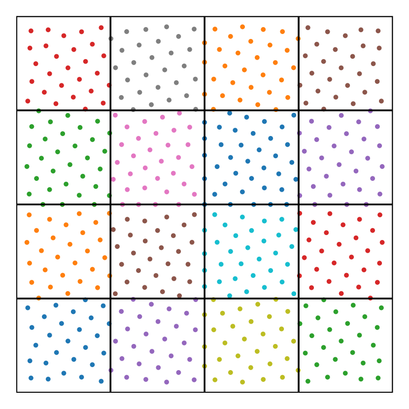
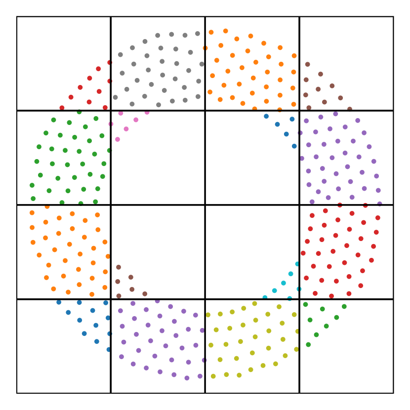
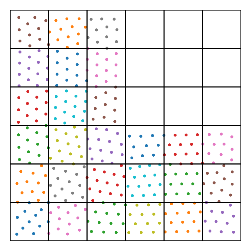
Figure 3: Illustration of uniform sampling on three different domains (square, annulus and L-shaped) and domain partitioning for the point source location ${\boldsymbol{\xi}}$. Left: $4\times 4$ blocks; middle: $4\times 4$ blocks; right: $6\times 6$ blocks.

4.5 Loss function

Define the training data for the set of GF-Nets: $\mathcal{S}^{k}=\mathcal{S}_{c}^{k}\cup\mathcal{S}_{b}^{k},$ where $\mathcal{S}_{c}^{k}=\{({\boldsymbol{x}},{\boldsymbol{\xi}})\in\mathcal{S}^{k}:{\boldsymbol{x}}\notin\partial\Omega\}$ and $\mathcal{S}_{b}^{k}=\{({\boldsymbol{x}},{\boldsymbol{\xi}})\in\mathcal{S}^{k}:{\boldsymbol{x}}\in\partial\Omega\}$, for $k=1,\ldots,K$. The $k$-th GF-Net is trained by minimizing the following total loss:

$$L({\boldsymbol{\Theta}}_{k})=L_{res}({\boldsymbol{\Theta}}_{k})+\lambda_{b}L_{bdry}({\boldsymbol{\Theta}}_{k})+\lambda_{s}L_{sym}({\boldsymbol{\Theta}}_{k}),$$ (8)

where

$$L_{res}({\boldsymbol{\Theta}}_{k}) =\frac{1}{|\mathcal{S}_{c}^{k}|}\sum_{({\boldsymbol{x}},{\boldsymbol{\xi}})\in\mathcal{S}_{c}^{k}}\left[\mathcal{L}G({\boldsymbol{x}},{\boldsymbol{\xi}};{\boldsymbol{\Theta}}_{k})-\rho({\boldsymbol{x}},{\boldsymbol{\xi}})\right]^{2},$$

$$L_{bdry}({\boldsymbol{\Theta}}_{k}) =\frac{1}{|\mathcal{S}_{b}^{k}|}\sum_{({\boldsymbol{x}},{\boldsymbol{\xi}})\in\mathcal{S}_{b}^{k}}\left[G({\boldsymbol{x}},{\boldsymbol{\xi}};{\boldsymbol{\Theta}}_{k})\right]^{2},$$

$$L_{sym}({\boldsymbol{\Theta}}_{k}) =\frac{1}{|\mathcal{S}_{c}^{k}|}\sum_{({\boldsymbol{x}},{\boldsymbol{\xi}})\in\mathcal{S}_{c}^{k}}\left[G({\boldsymbol{x}},{\boldsymbol{\xi}};{\boldsymbol{\Theta}}_{k})-G({\boldsymbol{\xi}},{\boldsymbol{x}};{\boldsymbol{\Theta}}_{k})\right]^{2}.$$

Here, $L_{res}({\boldsymbol{\Theta}}_{k})$ represents the pointwise PDE residual defined for each $({\boldsymbol{x}},{\boldsymbol{\xi}})$ pair, $L_{bdry}$ measures the errors on boundary, $L_{sym}({\boldsymbol{\Theta}}_{k})$ is introduced to enforce the intrinsic symmetry property of the Green’s function, and $\lambda_{b}$ and $\lambda_{s}$ are two hyperparameters for balancing the three terms. Note that the loss function (8) does not use any ground-truth data (i.e., the exact or certain approximate solution of the problem (3)).

5 A Fast Numerical Solver using GF-Nets

After training the set of GF-Nets, numerical solutions of the linear reaction-diffusion problem (2) can be directly computed based on the formula (4) using GF-Nets. In order to evaluate the integrals in (4) accurately, we apply numerical quadrature on triangular meshes. To this end, we generate a triangulation for the domain $\Omega$ consisting of triangles $\mathcal{T}_{q}=\{T_{l}\}$. Denote the intersection of the triangle edges with the domain boundary by ${\cal E}_{q}^{bdry}=\{E_{m}\}$. For any ${\boldsymbol{x}}\in\Omega$, we have

$$u({\boldsymbol{x}})\approx\sum_{T_{l}\in{\cal T}_{q}}I^{T_{l}}_{{\boldsymbol{\xi}},h}\big{[}f({\boldsymbol{\xi}})G({\boldsymbol{\xi}},{\boldsymbol{x}})\big{]}-\sum_{E_{m}\in{\cal E}_{q}^{bdry}}I^{E_{m}}_{{\boldsymbol{\xi}},h}\big{[}g({\boldsymbol{\xi}})a({\boldsymbol{\xi}})({\nabla_{{\boldsymbol{\xi}}}G}({\boldsymbol{\xi}},{\boldsymbol{x}})\cdot{\vec{\bf n}}_{{\boldsymbol{\xi}}})\big{]},$$ (9)

where $I^{T_{l}}_{{\boldsymbol{\xi}},h}[\cdot]$ denotes the numerical quadrature for evaluating $\int_{T_{l}}f({\boldsymbol{\xi}})G({\boldsymbol{\xi}},{\boldsymbol{x}})\,d{\boldsymbol{\xi}}$ and $I^{E_{m}}_{{\boldsymbol{\xi}},h}[\cdot]$ the quadrature for evaluating $\int_{E_{m}}g({\boldsymbol{\xi}})a({\boldsymbol{\xi}})({\nabla_{{\boldsymbol{\xi}}}G}({\boldsymbol{\xi}},{\boldsymbol{x}})\cdot{\vec{\bf n}}_{{\boldsymbol{\xi}}})\,dS({\boldsymbol{\xi}})$, respectively. For clarity, in Figure 4, we plot the quadrature points used in evaluating $I^{T_{l}}_{{\boldsymbol{\xi}},h}[\cdot]$ by a $4$-point Gaussian quadrature rule for triangular elements and $I^{E_{m}}_{{\boldsymbol{\xi}},h}[\cdot]$ by a $3$-point Gaussian quadrature rule on boundary segments. Due to the symmetry of $G({\boldsymbol{\xi}},{\boldsymbol{x}})$, the formula (9) can also be rewritten as an integration with respect to ${\boldsymbol{x}}$ instead of ${\boldsymbol{\xi}}$. The algorithm for solving the PDE problem (2) with GF-Nets is summarized in Algorithm 1.

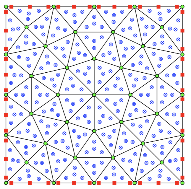
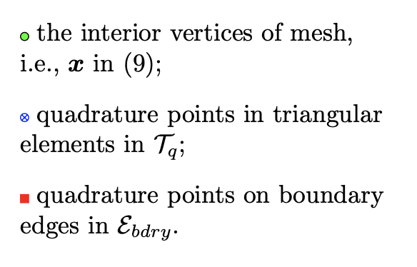
Figure 4: An illustration of the triangular mesh $\mathcal{T}_{q}$ and the quadrature points.

Algorithm 1 Solving the model problem (2) by GF-Nets

${\cal L}(\cdot)$, $f({\boldsymbol{x}})$ and $g({\boldsymbol{x}})$, the mesh $\mathcal{T}_{q}$, and an interior vertex $\widehat{{\boldsymbol{x}}}\in\Omega$ The PDE solution at $\widehat{{\boldsymbol{x}}}$: $u(\widehat{{\boldsymbol{x}}})$

1:  Generate sampling points $\mathcal{S}_{{\boldsymbol{\xi}}}$ and $\mathcal{S}_{{\boldsymbol{x}},{\boldsymbol{\xi}}}$.

2:  Apply the domain partition to divide $\Omega$ into $K$ blocks.

3:  for $k=1$ to $K$ do

4:     Collect the dataset in the $k$-th ${\boldsymbol{\xi}}$-block $\mathcal{S}^{k}=\{({\boldsymbol{x}},{\boldsymbol{\xi}}):{\boldsymbol{\xi}}\in\mathcal{S}_{\boldsymbol{\xi}}^{k},{\boldsymbol{x}}\in\mathcal{S}_{{\boldsymbol{x}},{\boldsymbol{\xi}}}\}$.

5:     Train the GF-Nets $G({\boldsymbol{x}},{\boldsymbol{\xi}};{\boldsymbol{\Theta}}_{k})$ by feeding all $({\boldsymbol{x}},{\boldsymbol{\xi}})\in\mathcal{S}^{k}$. 

6:  end for

7:  Check index $k$ of the ${\boldsymbol{\xi}}$-block which $\widehat{{\boldsymbol{x}}}$ locates in, $u(\widehat{{\boldsymbol{x}}})$ is computed from (9) using the $G({\boldsymbol{\xi}},{\boldsymbol{x}};{\boldsymbol{\Theta}}_{k})$.

6 Experimental results

In this section, we will investigate the performance of the proposed GF-Nets for approximating the Green’s functions (3) and its application for fast solution of the linear reaction-diffusion problem (2) by Algorithm 1.

6.1 Model parameters setting

Each GF-Net (associated with one block) in the experiments has $1$ auxiliary layer and $6$ hidden layers with $50$ neurons per layer, $\sigma({\boldsymbol{x}})=\sin({\boldsymbol{x}})$ is used as the activation function, $\lambda_{b}=400$ and $\lambda_{s}=1$ are taken in the loss function if not otherwisely specified, and $s=0.02$ is used in the Gaussian density function for approximating the Dirac delta function. For generating the training sample sets, we choose $c_{1}=5$ and $c_{2}=10$. Both the Adam and LBFGS optimizers are used in the training process. The purpose of the former is to provide a good initial guess to the latter. The Adam is run for up to $2\times 10^{4}$ steps with the training loss tolerance $\epsilon_{1}=0.5$ for possible early stopping, which is then followed by the LBFGS optimization for at most $1\times 10^{4}$ steps with the loss tolerance $\epsilon_{2}=1\times 10^{-4}$. The same settings are used in training all GF-Nets for ensuring them to possess the same level of accuracy.

To test the ability of the GF-Net for approximating the Green’s functions, we consider both the Poisson’s (pure diffusion) equations and a reaction-diffusion equation in the square $\Omega_{1}=[-1,1]^{2}$, the annulus $\Omega_{2}=B_{1}(\boldsymbol{0})\backslash B_{1/2}(\boldsymbol{0})$ with $B_{r}(\boldsymbol{0})$ denoting a circle centered at the origin with radius $r$, and the L-shaped domain $\Omega_{3}=[-1,1]^{2}\backslash[0,1]^{2}$, as shown in Figure 3. The numerical solutions of the PDEs at all the interior vertices $\mathcal{V}_{q}$ of the triangulation $\mathcal{T}_{q}$ are used for quantifying the performance, which are evaluated by the relative error in the $l_{2}$ norm:

$$Error =\frac{\big{(}\sum_{{\boldsymbol{x}}\in\mathcal{V}_{q}}\left|u_{e}({\boldsymbol{x}})-u_{p}({\boldsymbol{x}})\right|^{2}A_{\boldsymbol{x}}\big{)}^{1/2}}{\big{(}\sum_{{\boldsymbol{x}}\in\mathcal{V}_{q}}\left|u_{e}({\boldsymbol{x}})\right|^{2}A_{\boldsymbol{x}}\big{)}^{1/2}},$$

where $A_{\boldsymbol{x}}$ is the area of the dual cell related to the vertex ${\boldsymbol{x}}$, $u_{e}$ and $u_{p}$ denote the exact solution and approximate solution, respectively. All the experiments reported in this work are performed on an Ubuntu 18.04.3 LTS desktop with a 3.6GHz Intel Core i9-9900K CPU, 64GB DDR4 memory and Dual NVIDIA RTX 2080 GPUs.

6.2 Ablation study based on the Green’s function with a fixed point source

In this subsection, we choose the classic Poisson’s equation in a unit disk with a fixed point source ${\boldsymbol{\xi}}$ located at its center (i.e., the origin) to conduct ablation study of the proposed GF-Net, including the learning accuracy and the effect of using the symmetric loss term $L_{sym}$ in (8). Furthermore, detailed discussions about the choice of activation function and the effect of the auxiliary layer are presented in Appendix A.1. The analytic form of this specific Green’s function is given as below:

$$G_{\mathrm{e}}({\boldsymbol{x}},\boldsymbol{0})=-\frac{1}{4\pi}\ln{(x_{1}^{2}+x_{2}^{2})},\quad{\boldsymbol{x}}\in B_{1}(\boldsymbol{0}).$$

Since the point source ${\boldsymbol{\xi}}$ is fixed at the origin, only ${\boldsymbol{x}}$ needs to be sampled for training and we still adopt sampling strategy in Subsection 4.3 to obtain $\mathcal{S}_{{\boldsymbol{x}},\boldsymbol{0}}$, where three different levels of meshes $\{\mathcal{T}_{{\boldsymbol{x}}}\}_{i=1}^{3}$ with $\#\mathcal{V}_{\boldsymbol{x}}^{1}=31213,\#\mathcal{V}_{\boldsymbol{x}}^{2}=7842,\#\mathcal{V}_{\boldsymbol{x}}^{3}=1982$ are used. No domain partition is used since there is only one source point in this case.

Accuracy of learned Green’s function

To measure the accuracy of the predicted Green’s function produced by GF-Net, we calculate its relative $l_{2}$ error in $B_{\backslash\epsilon}(\boldsymbol{0})=B_{1}(\boldsymbol{0})\backslash B_{\epsilon}(\boldsymbol{0})$ with $\epsilon=3s$ to avoid the singularity at the origin. Quantitatively, we find the relative $l_{2}$ error is only about $1.29\times 10^{-3}$, which demonstrate very good performance of the proposed GF-Net for predicting the Green’s function. Figure 5 plots qualitative comparison of the Green’s function and its prediction by GF-Net, from which we see that the error mainly concentrates at the origin (the point source location) and decays rapidly to the boundary.

[$G_{\mathrm{e}}({\boldsymbol{x}},\boldsymbol{0})$] [$G_{\mathrm{a}}({\boldsymbol{x}},\boldsymbol{0})$] [$|G_{\mathrm{a}}({\boldsymbol{x}},\boldsymbol{0})-G_{\mathrm{e}}({\boldsymbol{x}},\boldsymbol{0})|$]

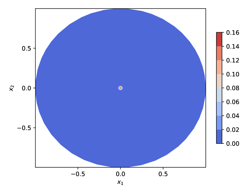
Figure 5: Numerical results for the Green’s function in the unit disk with the point source at the origin: the exact solution (left), the predicted solution by GF-Net (middle) and the numerical error (right).

Effect of the symmetric loss

Since the Green’s function is symmetric about ${\boldsymbol{x}}$ and ${\boldsymbol{\xi}}$, i.e., $G({\boldsymbol{x}},{\boldsymbol{\xi}})=G({\boldsymbol{\xi}},{\boldsymbol{x}})$ and such symmetric property is crucial to the quadrature formula (9), we introduce a symmetric error term into the total loss (8) so that the predicted Green’s function by GF-Net could preserve this property. To test the effect of this term to the learning outcome, we train the model in two ways: one includes the symmetric loss with $\lambda_{s}=1$, and the other excludes the symmetric loss from (8). The test results are shown in Figure 6, from which we see that adding the symmetric loss clearly improves the accuracy of predicted Green’s function.

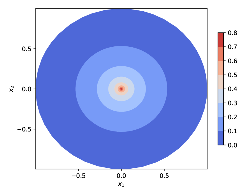
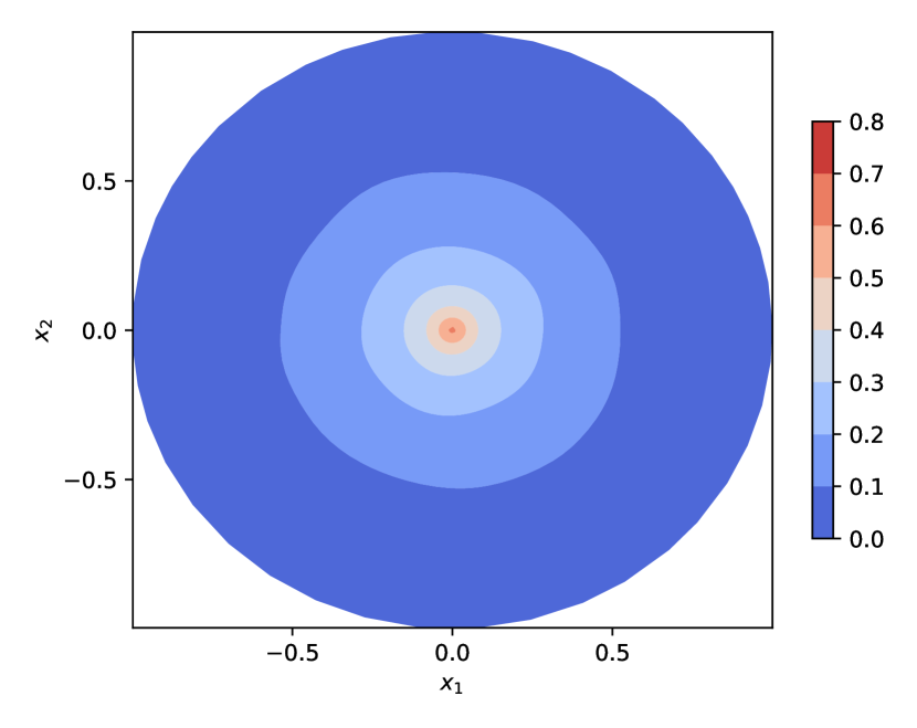
[$G_{\mathrm{e}}(\boldsymbol{0},{\boldsymbol{x}})$] [$G_{\mathrm{a}}(\boldsymbol{0},{\boldsymbol{x}})$ with $\lambda_{s}=1$] [$G_{\mathrm{a}}(\boldsymbol{0},{\boldsymbol{x}})$ with $\lambda_{s}=0$]

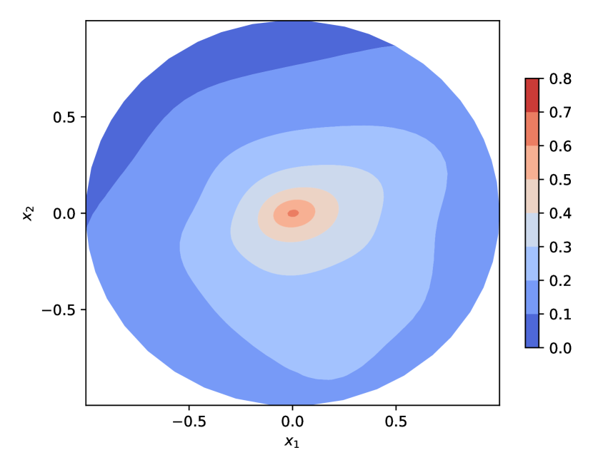
Figure 6: Numerical results for the symmetric property of Green’s function in the unit disk with the point source at the origin: the exact solution (left) and the predicted solutions by GF-Net with (middle) and without (right) the symmetric loss, respectively.

6.3 Ablation study based on Poisson’s equation with homogeneous and inhomogeneous boundary conditions

In this subsection, we investigate the effect of the domain partitioning strategies and the choice of the Gaussian parameter $s$ on the performance of the proposed GF-Net. For testing purpose, we consider the Poisson’s equation (i.e., the pure diffusion case with $a({\boldsymbol{x}})=1$ and $r({\boldsymbol{x}})=0$ in (1)) in the square $\Omega_{1}$. Both homogeneous and inhomogeneous Dirichlet boundary conditions are considered as below:

$$\textit{Case I (homogeneous BC)}:\quad u(x_{1},x_{2})=\sin(2\pi x_{1})\sin(2\pi x_{2}),$$

$$\textit{Case II (inhomogeneous BC)}:\quad u(x_{1},x_{2})=\cos(\pi x_{1})\cos(\pi x_{2}).$$

The source term $f(x_{1},x_{2})$ and the boundary values $g(x_{1},x_{2})$ are accordingly imposed to match the exact solution for interior and boundary points. $s=0.02$ and $s=0.015$ are used to examine how approxiamtion of Dirac delta function would affect the GF-Net. To train our GF-Net, we choose the mesh $\mathcal{T}_{\boldsymbol{\xi}}$ with $\#\mathcal{V}_{\boldsymbol{\xi}}=545$ for ${\boldsymbol{\xi}}$-samples and the related ${\boldsymbol{x}}$-samples are selected from three meshes $\{\mathcal{T}_{{\boldsymbol{x}}}^{i}\}_{i=1}^{3}$ with $\#\mathcal{V}_{\boldsymbol{x}}^{1}=32753,\#\mathcal{V}_{\boldsymbol{x}}^{2}=8265,\#\mathcal{V}_{\boldsymbol{x}}^{3}=2105$ to generate the sampling point set $\mathcal{S}$.

Effect of the domain partitioning strategy

We test the impact of the domain partitioning strategy on GF-Nets by considering $4\times 4,5\times 5$ and $6\times 6$ blocks. For the case of $4\times 4$ blocks, the predicted Green’s function with the source point ${\boldsymbol{\xi}}=(-0.8,0.8)$ is shown in Figure 9 (left). Moreover, the time costs of the training process under different domain partition settings are reported in Appendix A.2. The trained GF-Net is then applied for solving the Poisson’s equation. Three sets of quadrature points ($\#\mathcal{V}_{q}=145,289,545$) for numerical integration are considered and the resulted solution errors are reported in Table 1. It is easy to see that although different domain partitions are used, the numerical accuracy remains almost at the same level, with only slight improvements for larger partitions and more quadrature points in both cases. The predicted results by GF-Nets with $6\times 6$ subdomain blocks are presented in Figure 7 for visual illustration.

$\#\mathcal{V}_{q}$	Case I			Case II
	$4\times 4$	$5\times 5$	$6\times 6$	$4\times 4$	$5\times 5$	$6\times 6$
145	9.97e-3	9.63e-3	8.67e-3	6.00e-3	6.17e-3	5.78e-3
289	9.42e-3	8.91e-3	8.54e-3	4.46e-3	4.67e-3	5.32e-3
545	1.26e-2	1.19e-2	1.18e-2	4.31e-3	4.79e-3	4.23e-3

Table 1: Numerical errors of the predicted solutions to the Poisson’s equation in $\Omega_{1}$ obtained by using GF-Nets when three different domain partitions are used.

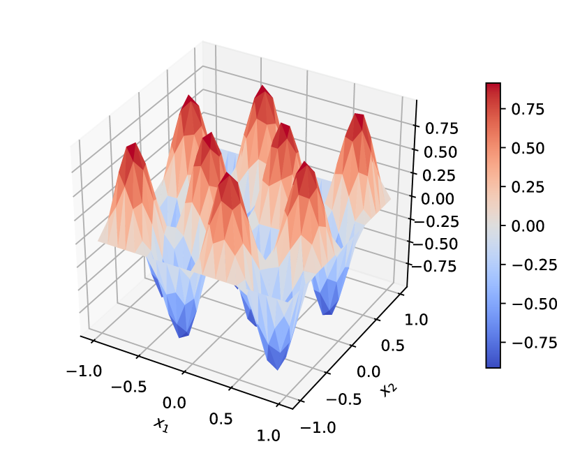
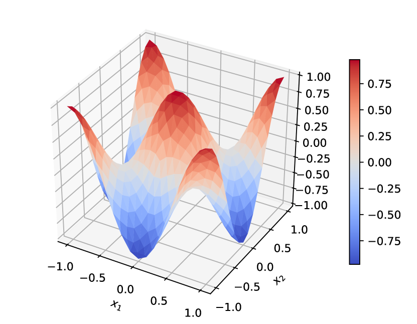
[Exact solution] [Predicted solution] [Error]

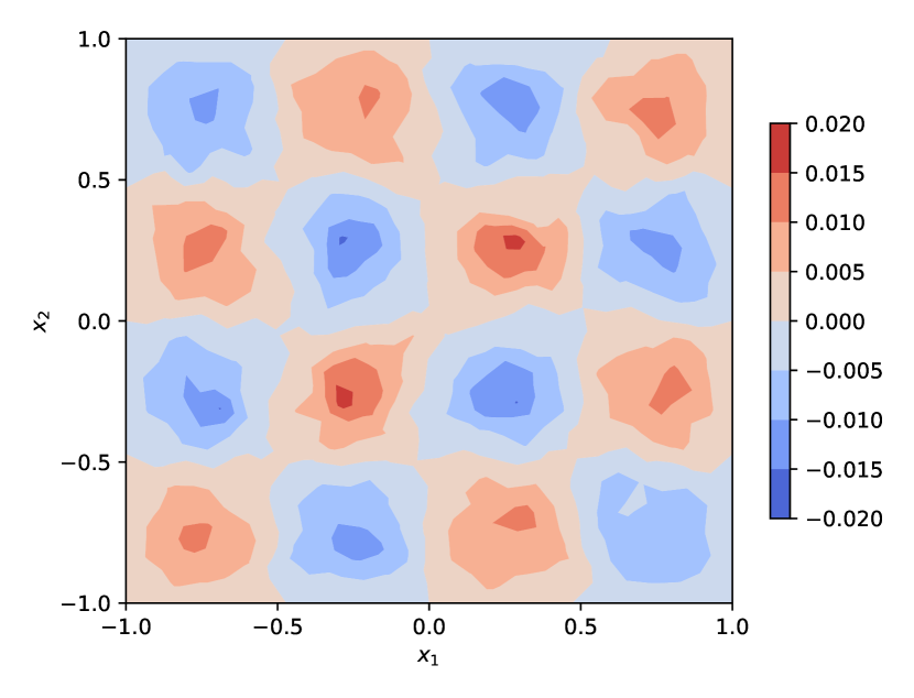
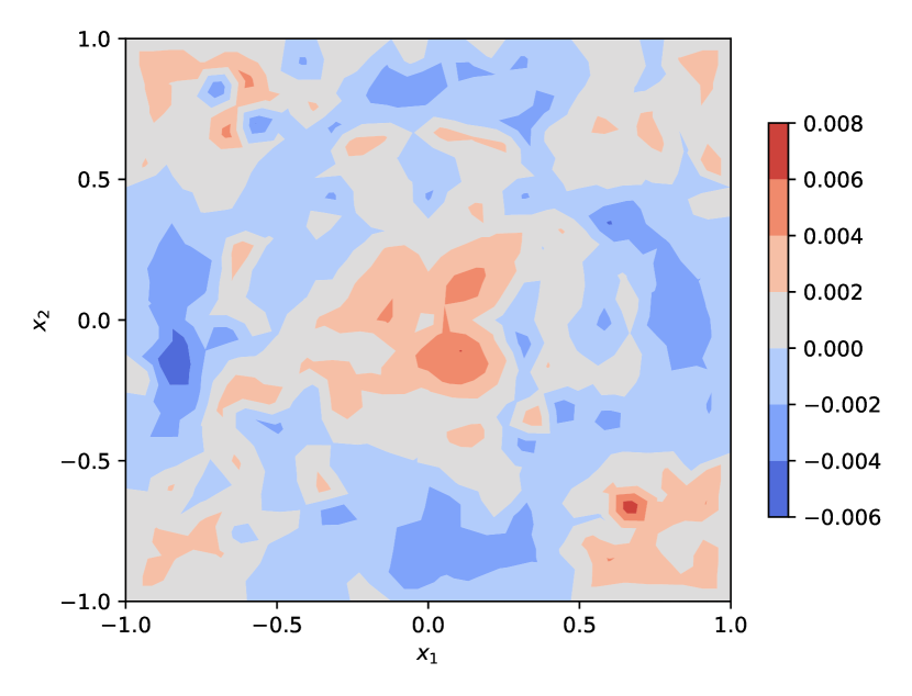
Figure 7: Numerical results for the solution of Poisson’s equation in $\Omega_{1}$ under Cases I (top row) and II (bottom row) obtained by using the trained GF-Nets with $6\times 6$ subdomain blocks. Left: the exact solutions; middle: the predicted solutions; right: the numerical errors.

Effect of the Gaussian parameter $s$

The value of the Gaussian parameter $s$ plays the most important role in accurately approximating the Dirac delta function. When the impulse source point ${\boldsymbol{\xi}}$ is positioned near the boundary, the Gaussian density function could not quickly decay to zero on the boundary if $s$ is not sufficiently small, which then causes large approximation errors due to the sudden truncation on the boundary (see the corresponding Gaussian density functions illustrated in Figure 8). To find how such truncation error would affect the accuracy of GF-Nets and corresponding fast solver for the Poisson’s equation, we repeatedly fine-tuned the obtained GF-Net from $s=0.02$ to $s=0.015$ based on two experimental observations: 1) Directly training GF-Nets with $s=0.015$ or even smaller could be unstable because training samples are insufficient to represent a sharp distribution change around the impulse source; 2) Even by applying the fine-tuning strategy, the training time for a smaller $s$ is much higher. The resulting numerical errors of the predicted solutions to the Poisson’s equation are compared in Table 2, where 545 training samples for ${\boldsymbol{\xi}}$ and $6\times 6$ subdomain block are used. It is observed that a smaller $s$ leads to more accurate results when the integral quadrature is accurate enough, but of course at the cost of longer training times and larger memory usages. Considering that the choice of $s=0.02$ already yields good approximations, we will stick with it in the subsequent numerical tests.

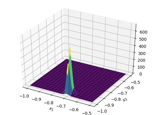
Figure 8: The approximations of the Dirac delta function with the source point at $(-0.7,-0.96)$ by the Gaussian density functions with $s=0.02$ (left), $s=0.015$ (middle) and $s=0.01$ (right), respectively.

$\#\mathcal{V}_{q}$	Case I		Case II
	$s=0.02$	$s=0.015$	$s=0.02$	$s=0.015$
145	8.67e-3	8.84e-3	5.78e-3	6.15e-3
289	8.54e-3	6.80e-3	5.32e-3	5.27e-3
545	1.18e-2	5.71e-3	4.23e-3	3.95e-3

Table 2: Numerical errors of the predicted solutions to the Poisson’s equation on $\Omega_{1}$ obtained by using GF-Nets with two different Gaussian parameter $s$.

6.4 More tests on Poisson’s equation

To further investigate the performance of the proposed GF-Net on non-convex domains, we also test the proposed GF-Nets and corresponding fast solver in the annulus $\Omega_{2}$ and the L-shaped domain $\Omega_{3}$. The same exact solutions as those (Cases I and II) in the previous subsection are considered. Some model parameters are listed in Table 3. Examples of the predicted Green’s functions $G({\boldsymbol{x}},{\boldsymbol{\xi}})$ in $\Omega_{2}$ with the source point ${\boldsymbol{\xi}}=(0,0.8)$ and in $\Omega_{3}$ with ${\boldsymbol{\xi}}=(-0.2,-0.2)$ are shown in Figure 9 (middle and right). As an example, numerical results for the solution of Poisson’s equation under Case II in $\Omega_{2}$ and $\Omega_{3}$ obtained using the trained GF-Nets are also plotted in Figure 10 for visual illustration. More related test results are provided in Appendix B.

Domain	$\#\mathcal{V}_{\boldsymbol{\xi}}$	$\#\mathcal{V}_{\boldsymbol{x}}^{1}$	$\#\mathcal{V}_{\boldsymbol{x}}^{2}$	$\#\mathcal{V}_{\boldsymbol{x}}^{3}$	$m$	$n$	$c_{1}$	$c_{2}$
$\Omega_{1}$	545	32753	8265	2105	4	4	5	10
$\Omega_{2}$	493	27352	6981	1819	4	4	5	10
$\Omega_{3}$	411	49663	6102	1565	6	6	5	10

Table 3: Parameter settings for the GF-Nets and the corresponding fast solver.

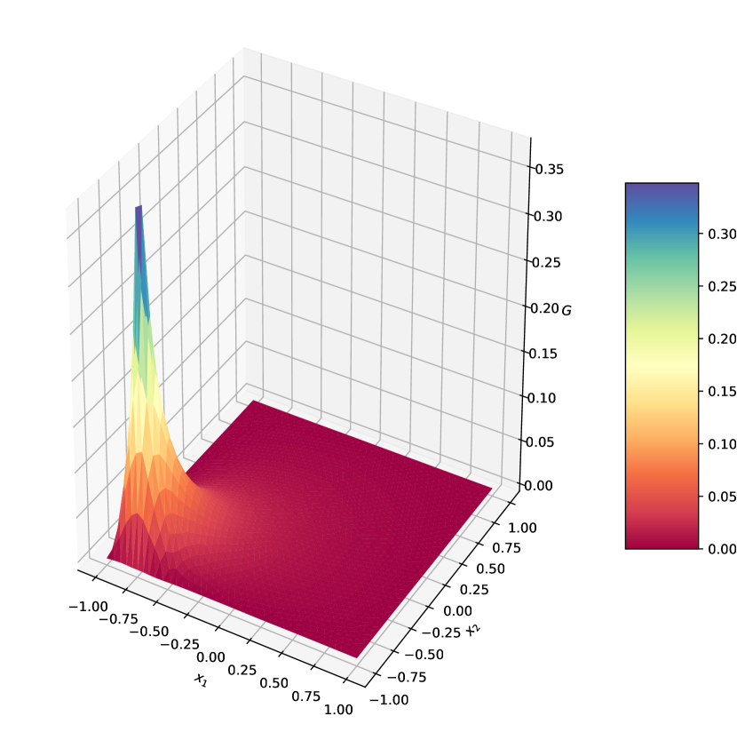
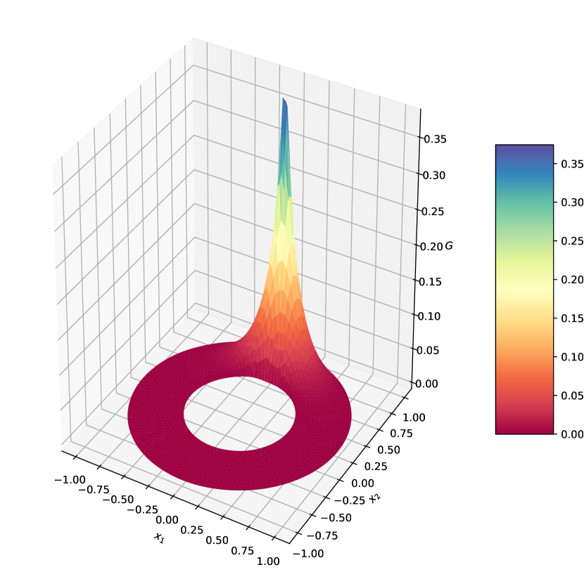
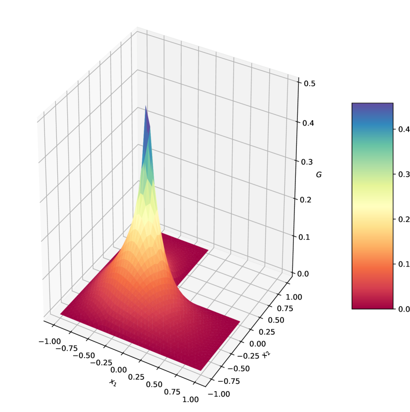
Figure 9: Predicted Green’s functions $G({\boldsymbol{x}},{\boldsymbol{\xi}})$ of the Poisson’s equation by GF-Nets. Left: $\Omega_{1}$ with ${\boldsymbol{\xi}}=(-0.8,-0.8)$; middle: $\Omega_{2}$ with ${\boldsymbol{\xi}}=(0,0.8)$; right: $\Omega_{3}$ with ${\boldsymbol{\xi}}=(-0.2,-0.2)$.

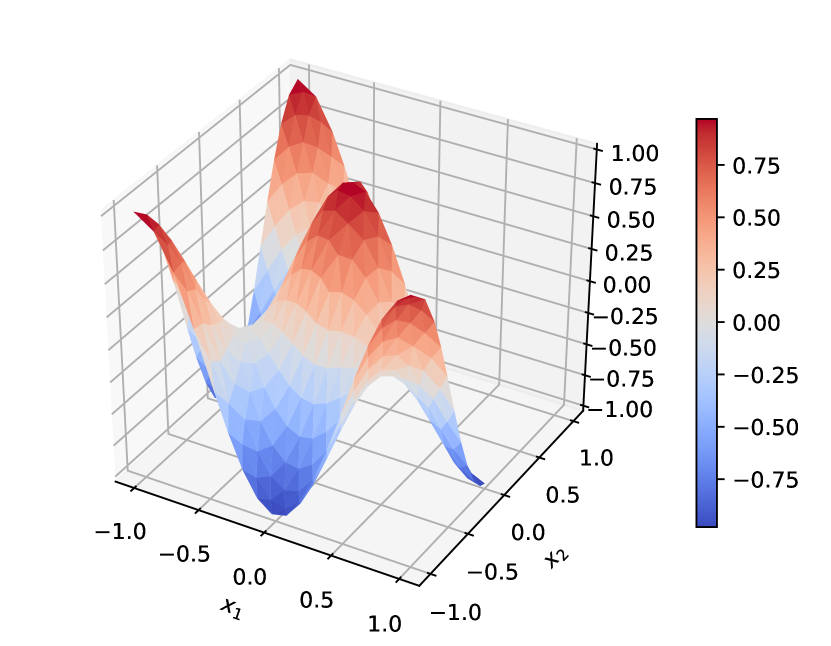
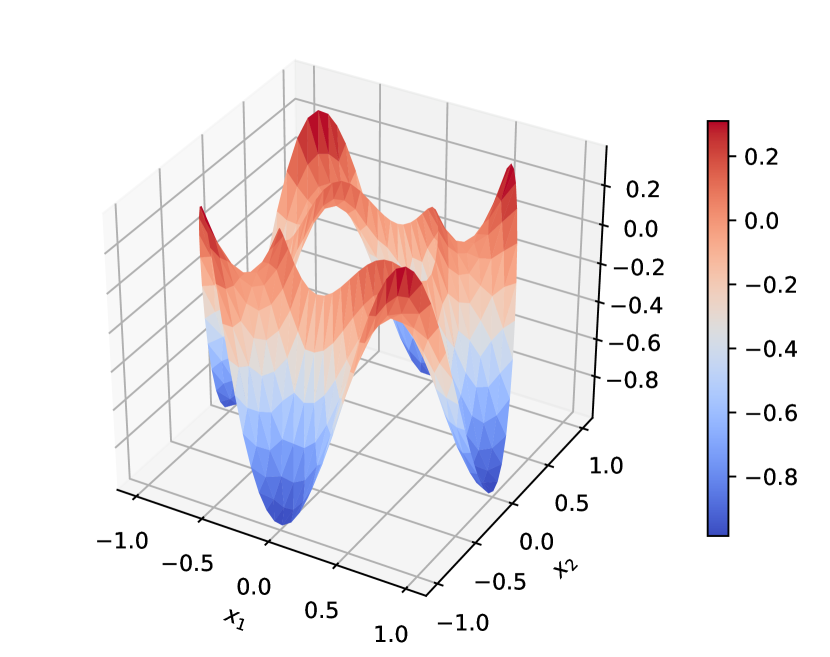
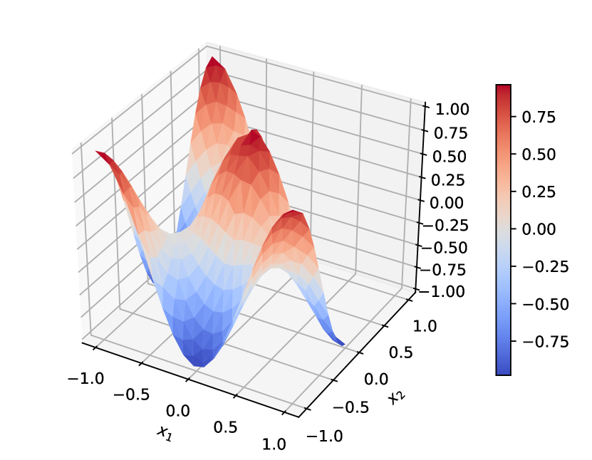
[Exact solution] [Predicted solution] [Error]

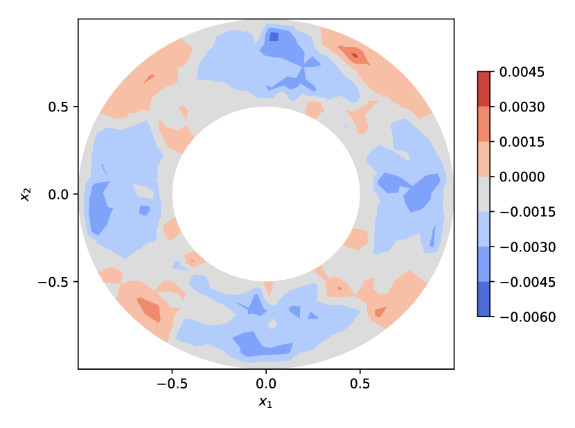
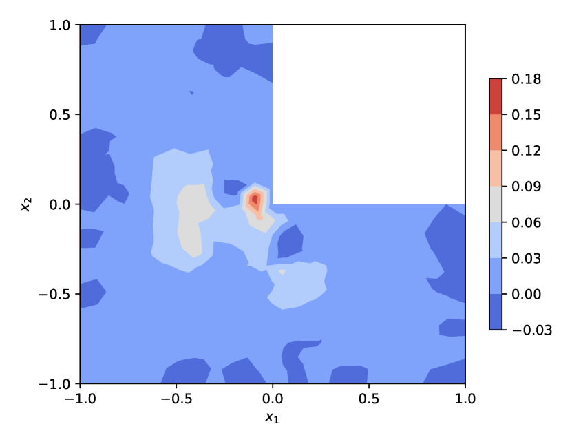
Figure 10: Numerical results for the solution of Poisson’s equation (Case II) in $\Omega_{2}$ (top row) and $\Omega_{3}$ (bottom row) obtained by using the trained GF-Nets. Left: the exact solutions; middle: the predicted solutions; right: the numerical errors.

To demonstrate the accuracy and efficiency of the proposed method as a numerical solver of the target PDE, we also compare the numerical solutions of the Poisson’s equation obtained by the trained GF-Nets with those of the classic finite element method (FEM) (implemented by FEniCS (Alnaes et al., 2015)) in the three domains $\Omega_{1},\Omega_{2}$ and $\Omega_{3}$. For a fair comparison, the FEM solutions are computed on the same meshes as those used for evaluating (9) with GF-Net. Numerical results for the Poisson’s equation, including solution errors and computation times (in seconds per GPU card), are reported in Table 4. We observe: 1) GF-Net is able to predict Green’s functions as well as FEM on all the three domains; 2) Evaluating the formula (9) on a finer quadrature mesh doesn’t improve the accuracy significantly, which indicates the numerical error is dominated by Green’s function approximation error in these cases; 3) the prediction accuracy of GF-Net can be better than that of FEM, at least on the relatively coarse grid; 4) the time costs of GF-Net are comparable to that of FEM, and furthermore, due to the superior parallelism for multiple GF-Nets, the computation time by GF-Nets can be be significantly reduced when multiple GPU cards are available.

$\Omega_{1}$: $\#\mathcal{V}_{q}$	Case I				Case II
	GF-Net	Time	FEM	Time	GF-Net	Time	FEM	Time
145	9.97e-3	0.11	2.36e-1	0.15	6.00e-3	0.11	6.35e-2	0.16
289	9.42e-3	0.18	1.15e-1	0.17	4.46e-3	0.18	2.67e-2	0.16
545	1.26e-2	0.40	5.19e-2	0.24	4.31e-3	0.34	1.46e-2	0.23
$\Omega_{2}$: $\#\mathcal{V}_{q}$	Case I				Case II
	GF-Net	Time	FEM	Time	GF-Net	Time	FEM	Time
143	1.27e-2	0.11	6.11e-1	0.16	8.14e-3	0.11	4.33e-2	0.15
224	1.42e-2	0.14	5.51e-1	0.17	8.27e-3	0.13	2.45e-2	0.16
493	1.36e-2	0.30	5.20e-1	0.22	4.53e-3	0.28	9.95e-3	0.30
$\Omega_{3}$: $\#\mathcal{V}_{q}$	Case I				Case II
	GF-Net	Time	FEM	Time	GF-Net	Time	FEM	Time
113	1.08e-2	0.17	2.48e-1	0.14	5.09e-2	0.17	6.11e-2	0.15
225	8.79e-3	0.24	1.13e-1	0.15	5.77e-2	0.23	2.65e-2	0.16
411	1.18e-2	0.38	5.37e-2	0.22	4.89e-2	0.37	1.46e-2	0.23

Table 4: Quantitative comparisons of solution errors and computation times (seconds) used by the GF-Net and the FEM for solving the Poisson’s equation.

6.5 Tests on the reaction-diffusion equation

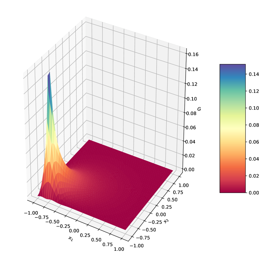
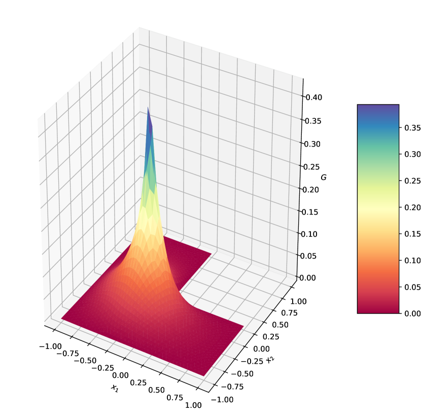
Figure 11: Predicted Green’s functions $G({\boldsymbol{x}},{\boldsymbol{\xi}})$ of the reaction-diffusion equation (10) by GF-Nets. Left: $\Omega_{1}$ with ${\boldsymbol{\xi}}=(-0.8,-0.8)$; middle: $\Omega_{2}$ with ${\boldsymbol{\xi}}=(0,0.8)$; right: $\Omega_{3}$ with ${\boldsymbol{\xi}}=(-0.2,-0.2)$.

We next test the following reaction-diffusion operator:

$${\cal L}(u)=-\nabla\cdot((1+2x_{2}^{2})\nabla u)+(1+x_{1}^{2})u$$ (10)

defined in the same three typical domains as before. The exact solution is chosen as $u(x_{1},x_{2})=e^{-(x_{1}^{2}+2x_{2}^{2}+1)}$ and the boundary conditions and the source term are determined accordingly. We use the same parameters as listed in Table 3. The predicted Green’s functions $G({\boldsymbol{x}},{\boldsymbol{\xi}})$ are shown in Figure 11 for the problem in $\Omega_{1}$ with the source point ${\boldsymbol{\xi}}=(-0.8,-0.8)$, $\Omega_{2}$ with ${\boldsymbol{\xi}}=(0,0.8)$, and $\Omega_{3}$ with ${\boldsymbol{\xi}}=(-0.2,-0.2)$. Numerical results for the predicted solutions to the reaction-diffusion equation (10) are reported in Table 5 and plotted in Figure 12. It is observed that the proposed GF-Net method again achieves similar numerical performance as to the Poisson’s equation.

$\Omega_{1}$		$\Omega_{2}$		$\Omega_{3}$
$\#\mathcal{V}_{q}$	$Error$	$\#\mathcal{V}_{q}$	$Error$	$\#\mathcal{V}_{q}$	$Error$
145	4.82e-3	143	7.89e-3	113	4.34e-2
289	4.52e-3	224	5.08e-3	225	5.10e-2
545	5.02e-3	493	2.23e-3	411	4.50e-2

Table 5: Numerical errors of the predicted solutions to the reaction-diffusion equation (10) in $\Omega_{1},\Omega_{2}$ and $\Omega_{3}$, obtained by using the trained GF-Nets.

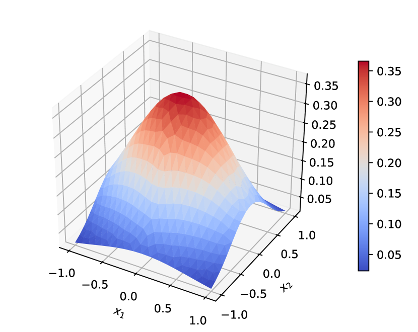
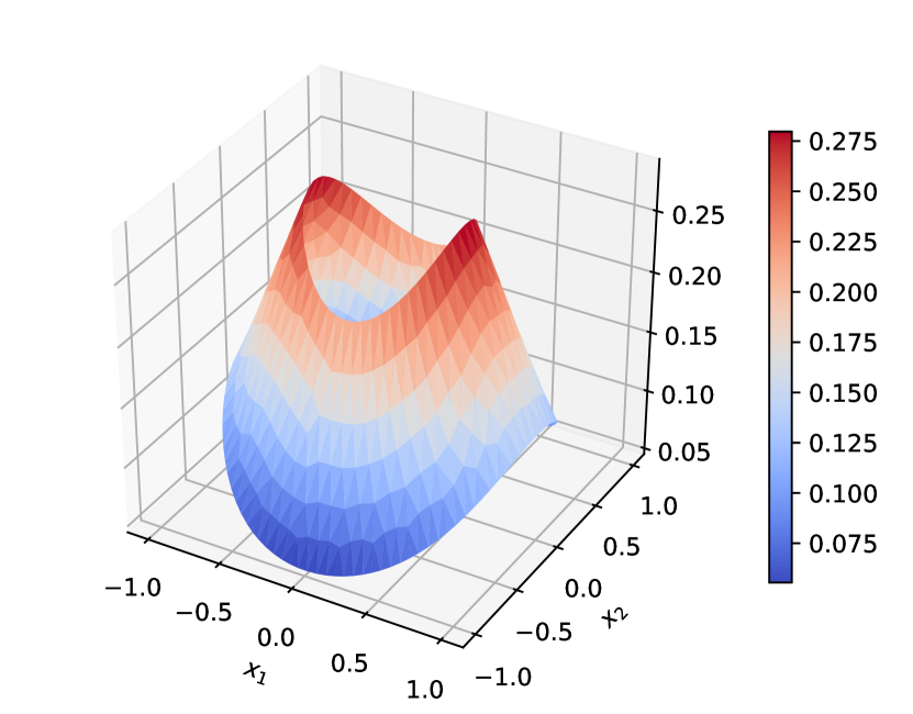
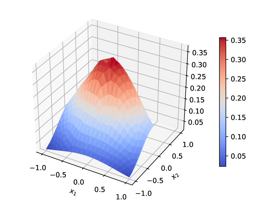
[Exact solution] [Predicted solution] [Error]

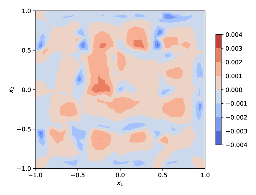
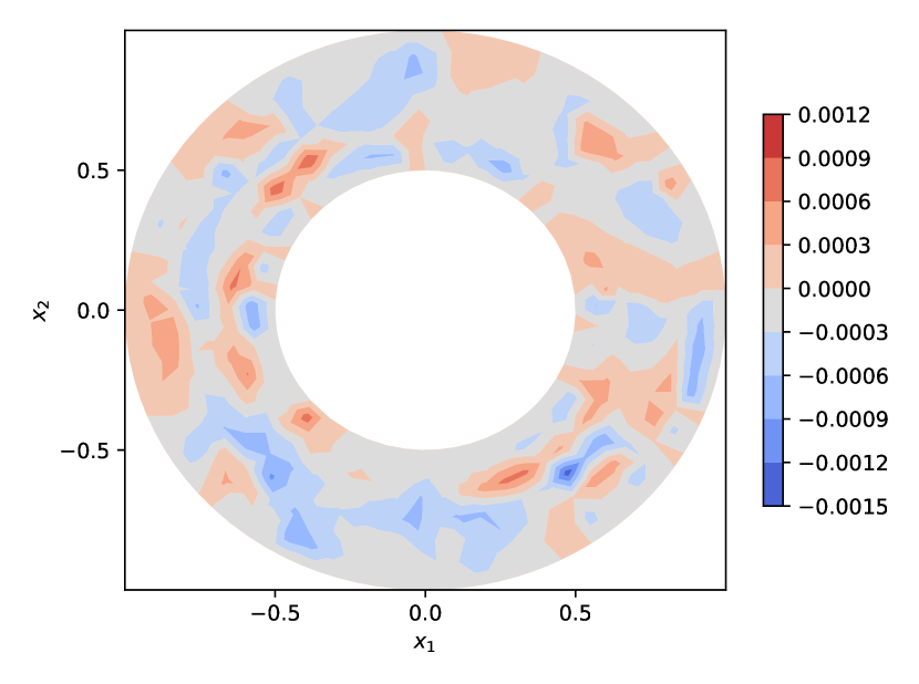
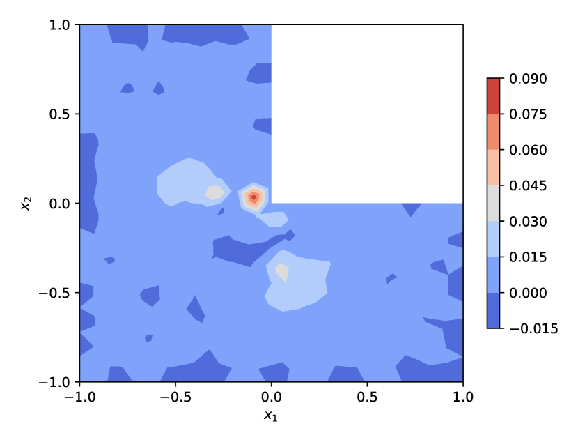
Figure 12: Numerical results for the solution of the reaction-diffusion equation (10) in $\Omega_{1}$ (top row), $\Omega_{2}$ (middle row) and $\Omega_{3}$ (bottom row) obtained by using the trained GF-Nets. Left: the exact solutions; middle: the predicted solutions; right: the numerical errors.

7 Conclusion

In this paper, we proposed the neural network model “GF-Net” to learn the Green’s functions of the classic linear reaction-diffusion equations in the unsupervised fashion. Our method overcomes the challenges faced by classic and machine learning approaches in determining the Green’s functions to differential operators in arbitrary domains. A series of procedures were taken to embed underlying properties of the Green’s functions into the GF-Net model. In particular, the symmetry feature is preserved by adding a penalization term to the loss function, and a domain decomposition approach is used for accelerating training and achieving better accuracy. The GF-Nets then can be used for fast numerical solutions of the target PDE subject to various sources and Dirichlet boundary conditions without the need of network retraining. Numerical experiments were also performed that show our GF-Nets can well handle the reaction-diffusion equations in arbitrary domains. Some interesting future works include the use of hard constraints for better match of the boundary values, the improvement of the sampling strategies for training GF-Nets for higher dimensional problems, and the extension of the proposed method to time-dependent and nonlinear PDEs.

X. Zhang’s work is partially supported by National Key Research and Development Program of China (2021YFD1900805-02). Z. Wang’s work is partially supported by U.S. National Science Foundation grant DMS-2012469. L. Ju’s work is partially supported by U.S. Department of Energy grant number DE-SC0022254.

Appendix A More Ablation Studies

A.1 Based on the Green’s function with a fixed point source

Effect of the activation function

Choosing a proper activation function sometimes could be a key part to the success of neural network models, thus we compare the effect of three commonly used activation functions ($\sin$, $\tanh$ and ${\rm sigmod}$) for training GF-Net and their performance in predicting the Green’s function. The training loss curves are displayed in Figure 13 (left), which shows that both $\tanh$ and $\sin$ work much better than ${\rm sigmoid}$ in terms of the decaying of training loss. Table 6 reports numerical errors of the predicted Green’s function. It is again observed that $\tanh$ and $\sin$ easily outperform ${\rm sigmoid}$, and $\sin$ performs the best among them. Hence, $\sin$ is selected as the activation function for GF-Net in all the experiments in this work.

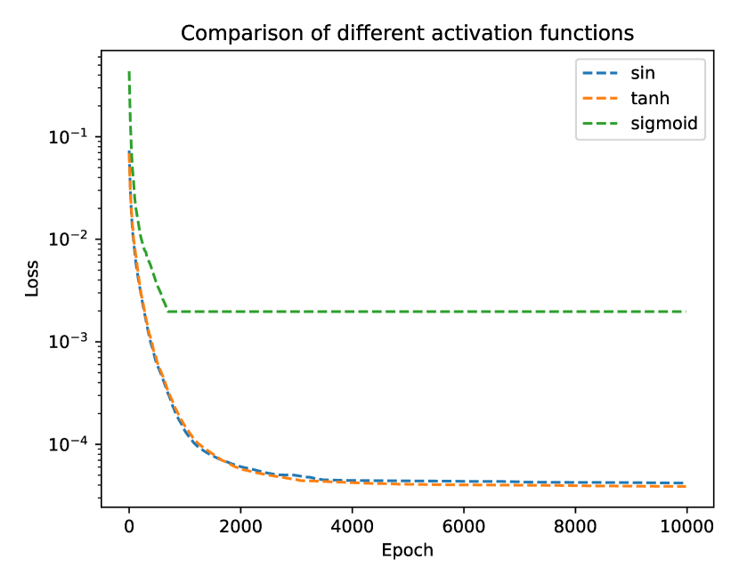
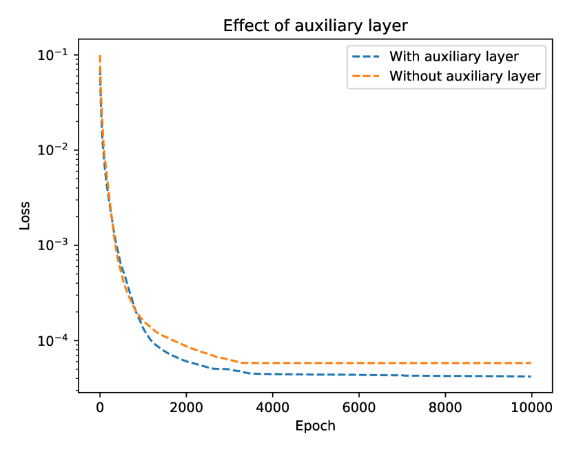
Figure 13: Comparison of different activation functions (left) and the effect of the auxiliary layer (right) for training the GF-Net in the unit disk with the point source at the origin. Note that only the LBFGS steps of the training process are shown here.

Effect of the auxiliary layer

We also compare the decaying of training loss with and without the auxiliary layer, see Figure 13 (right). It is easy to see that the training loss decays faster when the auxiliary layer is used.

Activation function	$\sin$	$\tanh$	sigmoid
Error	1.29e-3	1.38e-3	1.72e-2

Table 6: Numerical errors of the predicted Green’s function in the unit disk with the point source at the origin when different activation functions are used for GF-Net.

A.2 Training times with respect to the domain partitioning strategy

The computation costs of the training process under different domain partition settings are reported in Figure 14. It is observed that: 1) the training on blocks away from corners and boundaries of the domain are generally faster. In fact, it is found through experiments that the training processes for all interior blocks always terminates within several thousand LBFGS steps; 2) the training time per block decreases as the number of blocks increases, which implies this strategy is very suitable for parallel training when many GPU cards are available.

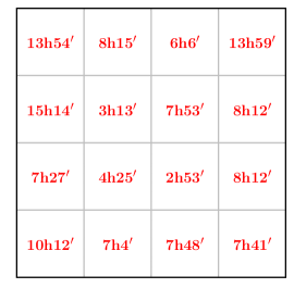
Figure 14: Training time of the GF-Net on each block for $4\times 4$ (left), $5\times 5$ (middle) and $6\times 6$ domain partitions (right).

Appendix B More Experiments for Poisson’s Equation

We investigate more on the application of the GF-Net to solve Poisson’s equation with Dirichlet boundary conditions. The three selected exact solutions are listed below:

$$u(x_{1},x_{2}) =x_{1}^{2}+x_{2}^{2}$$ (B.1)

$$u(x_{1},x_{2}) =\begin{cases}\cos(\pi x_{2}/2)&x_{1}\leq 0.6(x_{2}+1)\\ \cos(\pi x_{2}/2)+(x_{1}-0.6(x_{2}+1))^{\frac{3}{2}}&x_{1}>0.6(x_{2}+1)\end{cases}$$ (B.2)

$$u(x_{1},x_{2}) =e^{-100((x_{1}+0.5)^{2}+(x_{2}+0.5)^{2})}$$ (B.3)

which then accordingly determine the source term $f$ and the Dirichlet boundary condition $g$ for any given domain. The numerical results are shown in Figures 15, 16, 17, which are produced by the trained GF-Nets with the parameter settings given in Table 3. We observe that the approximation errors and simulation times remain at the similar magnitudes as those reported in Table 4.

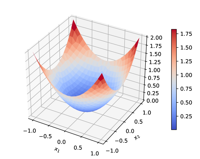
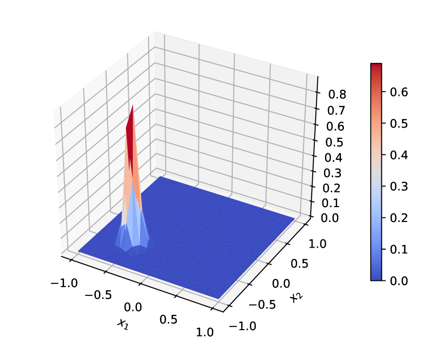
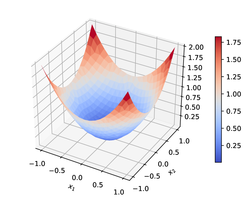
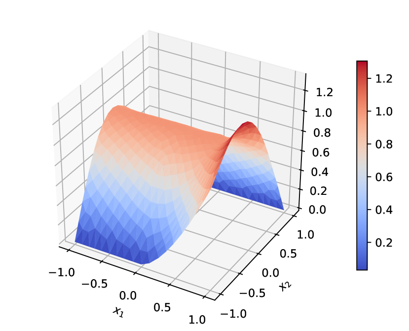
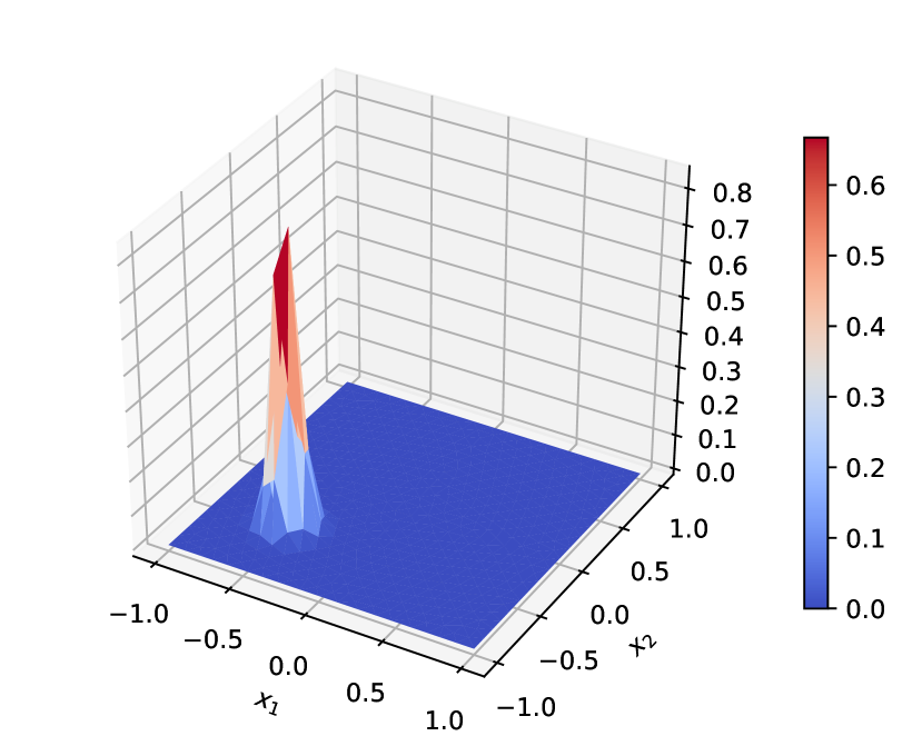
[Exact solutions] [Predicted solutions] [Errors]

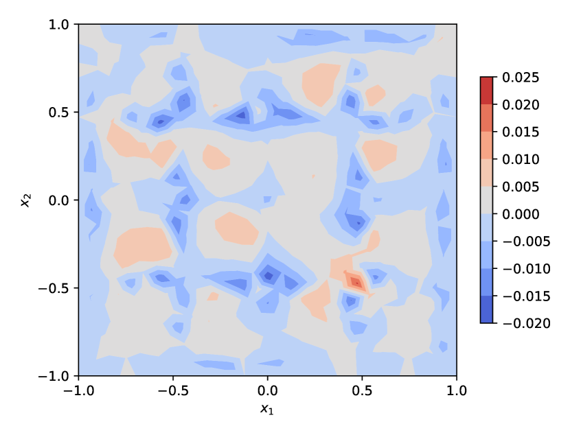
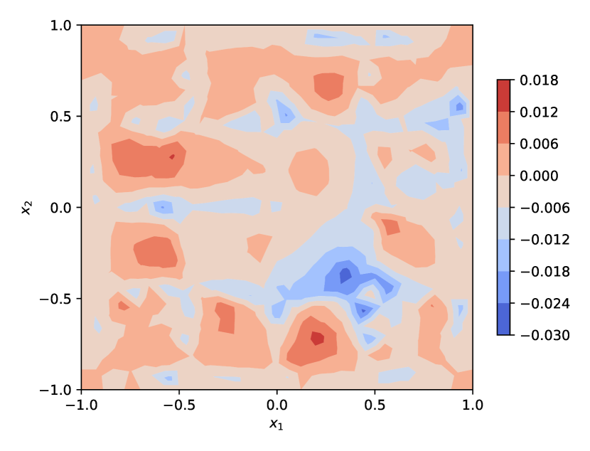
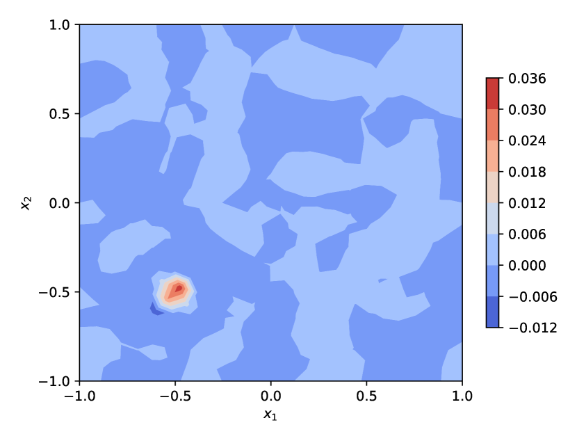
Figure 15: Numerical result for the solution of Poisson’s equation in $\Omega_{1}$ under different sets of source terms and boundary conditions, where the exact solutions (left), the predicted solutions by GF-Nets (middle), and the numerical errors (right) are presented. First row: Case (B.1); second row: Case (B.2); and last row: Case (B.3).

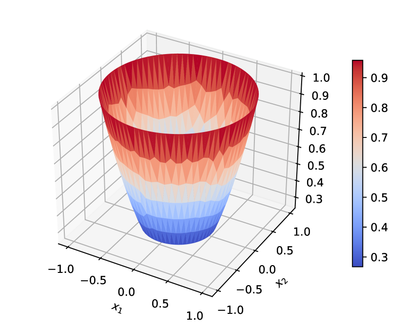
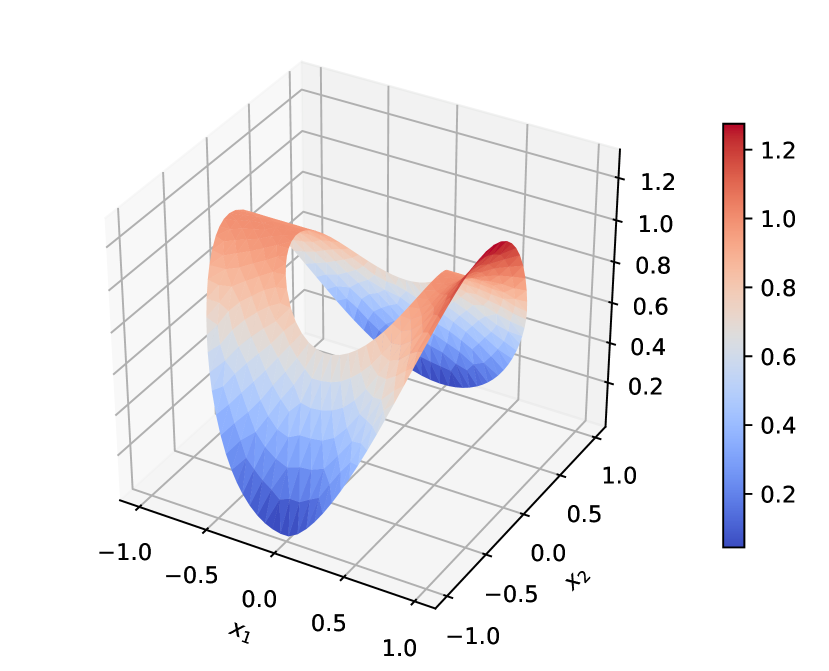
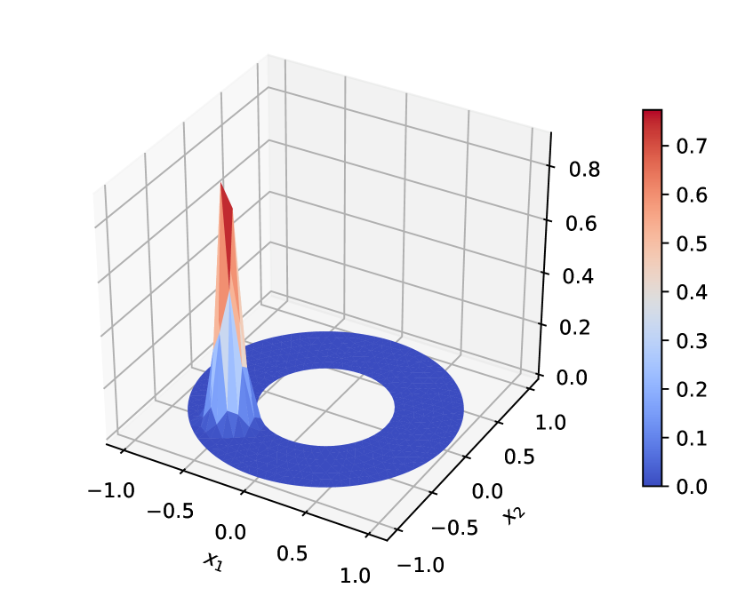
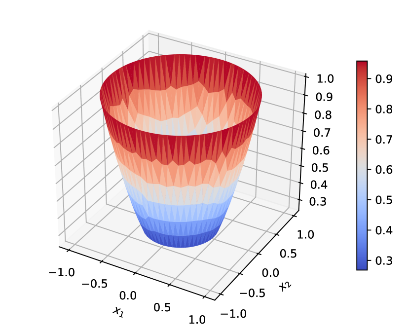
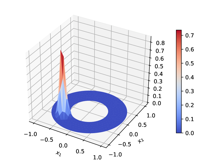
[Exact solution] [Predicted solution] [Error]

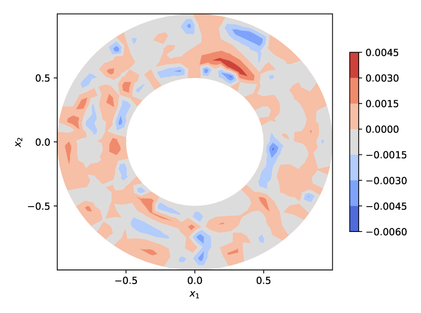
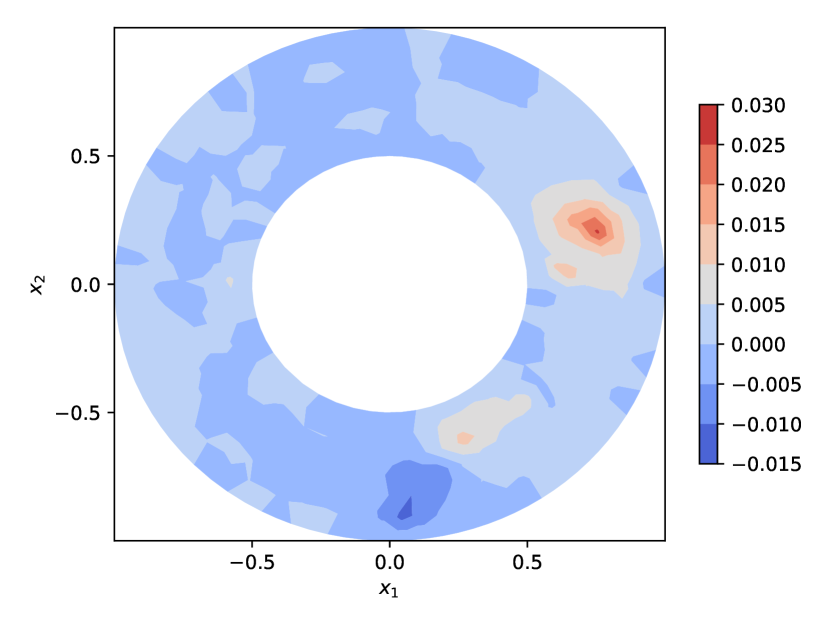
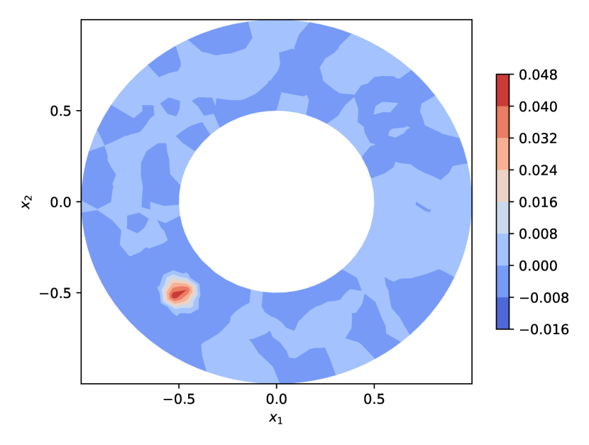
Figure 16: Numerical tests on Poisson’s equation in $\Omega_{2}$ under different sets of source terms and boundary conditions, where the exact solutions (left), the predicted solutions by GF-Nets (middle), and the numerical errors (right) are presented. First row: Case (B.1); second row: Case (B.2); and last row: Case (B.3).

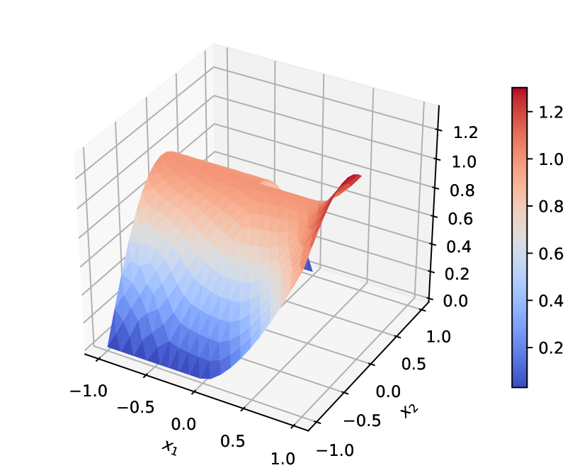
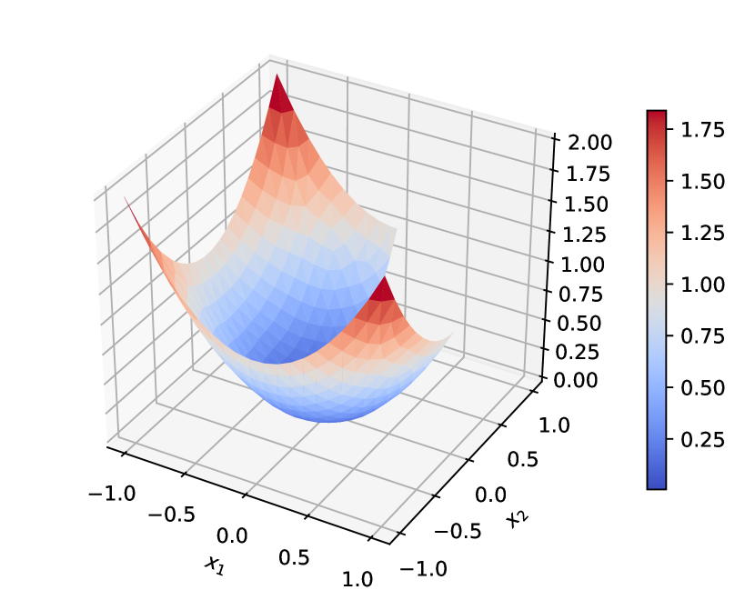
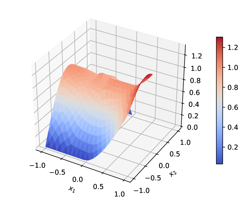
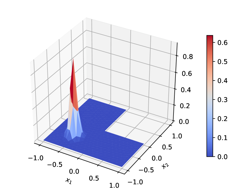
[Exact solution] [Predicted solution] [Error]

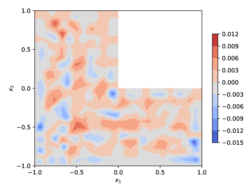
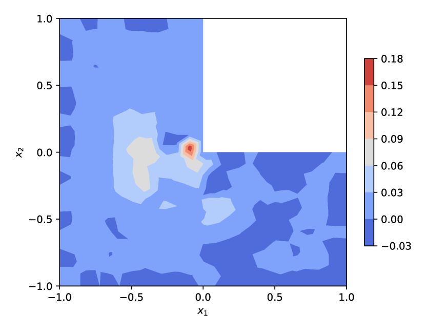
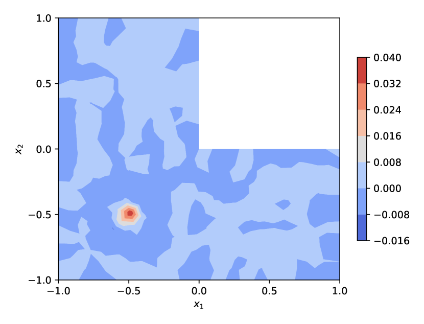
Figure 17: Numerical tests on Poisson’s equation in $\Omega_{3}$ under different sets of source terms and boundary conditions, where the exact solutions (left), the predicted solutions by GF-Nets (middle), and the numerical errors (right) are presented. First row: Case (B.1); second row: Case (B.2); and last row: Case (B.3).

References

- Alnaes et al. (2015) M. S. Alnaes, J. Blechta, J. Hake, A. Johansson, B. Kehlet, A. Logg, C. Richardson, J. Ring, M. E. Rognes, and G. N. Wells. The fenics project version 1.5. Archive of Numerical Software, 3(100):9–23, 2015.
- Anandkumar et al. (2020) Anima Anandkumar, Kamyar Azizzadenesheli, Kaushik Bhattacharya, Nikola Kovachki, Zongyi Li, Burigede Liu, and Andrew Stuart. Neural operator: Graph kernel network for partial differential equations. In ICLR 2020 Workshop on Integration of Deep Neural Models and Differential Equations, 2020.
- Anitescu et al. (2019) Cosmin Anitescu, Elena Atroshchenko, Naif Alajlan, and Timon Rabczuk. Artificial neural network methods for the solution of second order boundary value problems. Computers, Materials & Continua, 59(1):345–359, 2019.
- Boullé et al. (2022) Nicolas Boullé, Christopher J Earls, and Alex Townsend. Data-driven discovery of green’s functions with human-understandable deep learning. Scientific reports, 12(1):1–9, 2022.
- Chen and Chen (1995) Tianping Chen and Hong Chen. Universal approximation to nonlinear operators by neural networks with arbitrary activation functions and its application to dynamical systems. IEEE Transactions on Neural Networks, 6(4):911–917, 1995.
- Dissanayake and Phan-Thien (1994) M. Dissanayake and N. Phan-Thien. Neural-network-based approximations for solving partial differential equations. Communications in Numerical Methods in Engineering, 10(3):195–201, 1994.
- E and Yu (2018) Weinan E and Bing Yu. The deep Ritz method: a deep learning-based numerical algorithm for solving variational problems. Communication in Mathematics and Statistics, 6(1):1–12, 2018.
- Evans (1998) Lawrence C. Evans. Partial Differential Equations. American Mathematical Society, 1998.
- Gin et al. (2021) Craig R Gin, Daniel E Shea, Steven L Brunton, and J Nathan Kutz. Deepgreen: deep learning of green’s functions for nonlinear boundary value problems. Scientific Reports, 11(1):1–14, 2021.
- He and Xu (2019) Juncai He and Jinchao Xu. MgNet: A unified framework of multigrid and convolutional neural network. Science China Mathematics, 62:1331–1354, 2019.
- Huang et al. (2021) Xiang Huang, Hongsheng Liu, Beiji Shi, Zidong Wang, Kang Yang, Yang Li, Bingya Weng, Min Wang, Haotian Chu, Jing Zhou, Fan Yu, Bei Hua, Lei Chen, and Bin Dong. Solving partial differential equations with point source based on physics-informed neural networks. arXiv preprint arXiv.2111.01394, 2021.
- Ju (2007) Lili Ju. Conforming centroidal voronoi delaunay triangulation for quality mesh generation. International Journal of Numerical Analysis and Modeling, 4:531–546, 2007.
- Khoo et al. (2021) Yuehaw Khoo, Jianfeng Lu, and Lexing Ying. Solving parametric pde problems with artificial neural networks. European Journal of Applied Mathematics, 32(3):421–435, 2021.
- Kissas et al. (2022) Georgios Kissas, Jacob Seidman, Leonardo Ferreira Guilhoto, Victor M Preciado, George J Pappas, and Paris Perdikaris. Learning operators with coupled attention. arXiv preprint arXiv:2201.01032, 2022.
- Krishnapriyan et al. (2021) Aditi Krishnapriyan, Amir Gholami, Shandian Zhe, Robert Kirby, and Michael W Mahoney. Characterizing possible failure modes in physics-informed neural networks. Advances in Neural Information Processing Systems, 34, 2021.
- Lagaris et al. (1998) Isaac E Lagaris, Aristidis Likas, and Dimitrios I Fotiadis. Artificial neural networks for solving ordinary and partial differential equations. IEEE transactions on neural networks, 9(5):987–1000, 1998.
- Lanthaler et al. (2022) Samuel Lanthaler, Siddhartha Mishra, and George E Karniadakis. Error estimates for deeponets: A deep learning framework in infinite dimensions. Transactions of Mathematics and Its Applications, 6(1):tnac001, 2022.
- Lee and Carlberg (2020) Kookjin Lee and Kevin Carlberg. Model reduction of dynamical systems on nonlinear manifolds using deep convolutional autoencoders. Journal of Computational Physics, 404:108973, 2020.
- Li et al. (2020) Zongyi Li, Nikola Kovachki, Kamyar Azizzadenesheli, Burigede Liu, Andrew Stuart, Kaushik Bhattacharya, and Anima Anandkumar. Multipole graph neural operator for parametric partial differential equations. Advances in Neural Information Processing Systems, 33:6755–6766, 2020.
- Li et al. (2021a) Zongyi Li, Nikola Borislavov Kovachki, Kamyar Azizzadenesheli, Kaushik Bhattacharya, Andrew Stuart, Anima Anandkumar, et al. Fourier neural operator for parametric partial differential equations. In International Conference on Learning Representations, 2021a.
- Li et al. (2021b) Zongyi Li, Hongkai Zheng, Nikola Kovachki, David Jin, Haoxuan Chen, Burigede Liu, Kamyar Azizzadenesheli, and Anima Anandkumar. Physics-informed neural operator for learning partial differential equations. arXiv preprint arXiv:2111.03794, 2021b.
- Long et al. (2018) Zichao Long, Yiping Lu, Xianzhong Ma, and Bin Dong. PDE-Net: Learning PDEs from data. In International Conference on Machine Learning, pages 3214–3222, 2018.
- Long et al. (2019) Zichao Long, Yiping Lu, and Bin Dong. PDE-Net 2.0: Learning PDEs from data with a numeric-symbolic hybrid deep network. Journal of Computational Physics, 399:108925, 2019.
- Lu et al. (2021a) Lu Lu, Pengzhan Jin, Guofei Pang, Zhongqiang Zhang, and George Em Karniadakis. Learning nonlinear operators via DeepONet based on the universal approximation theorem of operators. Nature Machine Intelligence, 3(3):218–229, 2021a.
- Lu et al. (2021b) Lu Lu, Xuhui Meng, Zhiping Mao, and George Em Karniadakis. Deepxde: A deep learning library for solving differential equations. SIAM Review, 63(1):208–228, 2021b.
- Lu et al. (2021c) Lu Lu, Raphael Pestourie, Wenjie Yao, Zhicheng Wang, Francesc Verdugo, and Steven G Johnson. Physics-informed neural networks with hard constraints for inverse design. SIAM Journal on Scientific Computing, 43(6):B1105–B1132, 2021c.
- McKay et al. (1979) M.D. McKay, R.J. Beckman, and W.J. Conover. A comparison of three methods for selecting values of input variables in the analysis of output from a computer code. Technometrics. American Statistical Association, 21(2):239–245, 1979.
- Mücke et al. (2019) Nikolaj Takata Mücke, Lasse Hjuler Christiansen, Allan Peter Engsig-Karup, and John Bagterp Jørgensen. Reduced order modeling for nonlinear pde-constrained optimization using neural networks. In 2019 IEEE 58th Conference on Decision and Control (CDC), pages 4267–4272. IEEE, 2019.
- Nabian and Meidani (2019) Mohammad Amin Nabian and Hadi Meidani. A deep learning solution approach for high-dimensional random differential equations. Probabilistic Engineering Mechanics, 57:14–25, 2019.
- Nagoor Kani and Elsheikh (2017) J Nagoor Kani and Ahmed H Elsheikh. Dr-rnn: a deep residual recurrent neural network for model reduction. arXiv preprint arXiv:1709.00939, 2017.
- Pang et al. (2019) Guofei Pang, Lu Lu, and George Em Karniadakis. fPINNs: Fractional physics-informed neural networks. SIAM Journal on Scientific Computing, 41(4):A2603–A2626, 2019.
- Raissi et al. (2019) Maziar Raissi, Paris Perdikaris, and George E Karniadakis. Physics-informed neural networks: A deep learning framework for solving forward and inverse problems involving nonlinear partial differential equations. Journal of Computational Physics, 378:686–707, 2019.
- Raissi et al. (2020) Maziar Raissi, Alireza Yazdani, and George Em Karniadakis. Hidden fluid mechanics: Learning velocity and pressure fields from flow visualizations. Science, 367(6481):1026–1030, 2020.
- Ross (1976) Sheldon Ross. A First Course in Probability. MacMillan Publishing Company, 1976.
- San et al. (2019) Omer San, Romit Maulik, and Mansoor Ahmed. An artificial neural network framework for reduced order modeling of transient flows. Communications in Nonlinear Science and Numerical Simulation, 77:271–287, 2019.
- Sirignano and Spiliopoulos (2018) Justin Sirignano and Konstantinos Spiliopoulos. DGM: A deep learning algorithm for solving partial differential equations. Journal of Computational Physics, 375:1339–1354, 2018.
- Sun et al. (2020) Luning Sun, Han Gao, Shaowu Pan, and Jian-Xun Wang. Surrogate modeling for fluid flows based on physics-constrained deep learning without simulation data. Computer Methods in Applied Mechanics and Engineering, 361:112732, 2020.
- Wang et al. (2021) Sifan Wang, Hanwen Wang, and Paris Perdikaris. Learning the solution operator of parametric partial differential equations with physics-informed deeponets. Science Advances, 7(40):eabi8605, 2021.
- Yang et al. (2020) Liu Yang, Dongkun Zhang, and George Em Karniadakis. Physics-informed generative adversarial networks for stochastic differential equations. SIAM Journal on Scientific Computing, 42(1):A292–A317, 2020.
- Zang et al. (2020) Yaohua Zang, Gang Bao, Xiaojing Ye, and Haomin Zhou. Weak adversarial networks for high-dimensional partial differential equations. Journal of Computational Physics, 411:109409, 2020.
- Zhang et al. (2019) Dongkun Zhang, Lu Lu, Ling Guo, and George Em Karniadakis. Quantifying total uncertainty in physics-informed neural networks for solving forward and inverse stochastic problems. Journal of Computational Physics, 397:108850, 2019.
- Zhang et al. (2020) Dongkun Zhang, Ling Guo, and George Em Karniadakis. Learning in modal space: Solving time-dependent stochastic pdes using physics-informed neural networks. SIAM Journal on Scientific Computing, 42(2):A639–A665, 2020.
- Zhao and Wright (2021) Jia Zhao and Colby L Wright. Solving allen-cahn and cahn-hilliard equations using the adaptive physics informed neural networks. Communications in Computational Physics, 29:930–954, 2021.
- Zhu et al. (2019) Yinhao Zhu, Nicholas Zabaras, Phaedon-Stelios Koutsourelakis, and Paris Perdikaris. Physics-constrained deep learning for high-dimensional surrogate modeling and uncertainty quantification without labeled data. Journal of Computational Physics, 394:56–81, 2019.