Cooperative Multi-Agent Path Finding: Beyond Path Planning and Collision Avoidance

Abstract

We introduce the Cooperative Multi-Agent Path Finding (Co-MAPF) problem, an extension to the classical MAPF problem, where cooperative behavior is incorporated. In this setting, a group of autonomous agents operate in a shared environment and have to complete cooperative tasks while avoiding collisions with the other agents in the group. This extension naturally models many real-world applications, where groups of agents are required to collaborate in order to complete a given task. To this end, we formalize the Co-MAPF problem and introduce Cooperative Conflict-Based Search (Co-CBS), a CBS-based algorithm for solving the problem optimally for a wide set of Co-MAPF problems. Co-CBS uses a cooperation-planning module integrated into CBS such that cooperation planning is decoupled from path planning. Finally, we present empirical results on several MAPF benchmarks demonstrating our algorithm’s properties.

I Introduction and Related Work

The Multi-Agent Path-Finding (MAPF) problem is a special and important type of the more general Multi-Agent Planning (MAP) problem [1]. In MAPF [2], the task is to find paths for each agent in a group, from a start to a goal location, where interactions between agents are restricted to collision avoidance, as agents move in a shared environment. While relevant to many real-world applications, such as warehouse automation [3], autonomous vehicles [4, 5] and robotics [6], recent research in the field has focused on expanding the classical MAPF framework to fit more real-world applications [7, 8, 9].

A main research direction towards the real-world applicability of MAPF problems is the problem of lifelong MAPF, also known as the Multi-Agent Pickup and Delivery (MAPD) problem. In this problem, a group of autonomous agents operate in a shared environment to complete a stream of incoming tasks, each with start and goal locations, while avoiding collisions with each others [10, 11]. A similar problem, studied by Ma et al. [12] is the package-exchange robot-routing problem (PERR) where payload exchanges and transfers are allowed thus enabling the modelling of more general transportation problems.

In this work, we introduce the Cooperative-MAPF (Co-MAPF) framework, a MAPF extension, in which a group of agents collaborate towards completing a cooperative task. The classical MAPF problem is inherently cooperative, since each agent has to arrive at its goal, without colliding with other agents. However, in many real-world applications, agents that operate in a shared environment are often heterogeneous [13] and may have a different set of abilities and restrictions. Therefore, in the Co-MAPF framework, achieving goals and completing tasks may not depend only on avoiding collisions between agents, but also on actively coordinating their actions. Simply put, we may want agents not just to “not interrupt” each other, but also help each other achieve their goals. We term this a truly cooperative setting.

Our motivating problem is taken from the warehouse-automation domain [3]. In this problem, storage locations host inventory pods that hold goods of different kinds. Robots operate autonomously in the warehouse, picking up and carrying inventory pods to designated drop-off locations, where goods are manually taken off the pods for packaging. In this scenario, the robot’s main task is to transport the pods around the warehouse, and we refer to robots executing such tasks as transfer units. Research in a different, yet closely-related area, has studied the problem of autonomous robotic arms capable of picking-up a specific item from an inventory pod [14]. We refer to a moving robot with such arm as a grasp unit. This motivates the investigation of an improved warehouse scenario, where robots of two types, grasp and transfer units, can work together in coordination (for example, by scheduling a meeting between them) to improve some optimization objective. For instance, the number of completed tasks for a given time period. This motivating example is depicted in Fig. 1.

We incorporate a truly cooperative behavior to classical MAPF by assigning cooperative tasks (rather than goals) to agents, similar to (non-cooperative) tasks defined in the MAPD literature [10, 11]. Agents cooperate in the context of these cooperative tasks, and are only able to complete tasks by coordinating their actions and goals with each other.

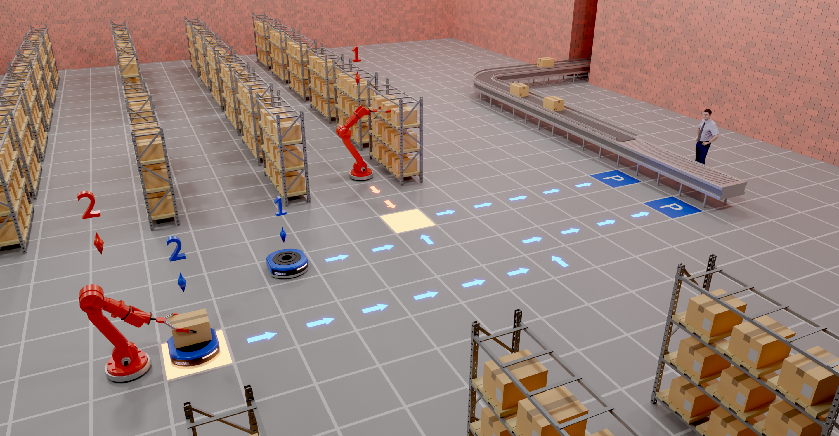
Figure 1: Two pairs of robots operate in a warehouse–two grasp units and two transfer units. Grasp unit $\#1$ arrived at the task start location, i.e., next to the shelf. It will pick up the box and then drive to the meeting location (marked with a yellow square) to transfer the box to transfer unit $\#1$. The transfer unit has a path (marked with blue arrows) to the meeting point, and from there to the task goal (the P square), where the box will be picked by a human employee. The second pair of robots ($\#2$) are at their meeting location.

We suggest a formulation to the Co-MAPF problem which is derived from the classical MAPF formulation [2]. In addition, we discuss differences and further extensions to the Co-MAPF framework which can be used towards achieving more cooperative capabilities in a MAPF problem. In the suggested formulation, presented in Section II, there is more than one set of agents, possibly representing heterogeneous real-world agents, and we specifically focus on the case of two sets of agents. The cooperation between agents is restricted to the form of meetings, where agents have to schedule a meeting location and time to complete a task. We also discuss other forms of agent interactions, and generalizations to the suggested formulation. Besides the aforementioned warehouse problem, more real-world problems can be modeled using the Co-MAPF framework, such as the involvement of aerial robots in fulfilment centers [15], the truck-and-drone “last-mile” delivery problem [16] and multi-drone delivery using transit networks [17].

Based on the suggested formulation, we introduce (in Section III) Cooperative Conflict-Based Search (Co-CBS), an optimal three-level algorithm that is heavily based on two previously-suggested optimal algorithms: the well-known Conflict-Based Search (CBS) [18] for solving a classical MAPF problem and the Conflict-Based Search with Optimal Task Assignment (CBS-TA) [19] for solving the anonymous MAPF problem, where we also need to assign goals (or tasks) to each agent. We define, similarly to MAPD problems [20, 10], a notion of well-formed problem instances, representing realistic and practical environments in MAPF domains, for which a solution to the Co-MAPF problem is guaranteed to exist. Finally, we introduce two improvements to the basic version of Co-CBS.

For clarity of exposition, the description of our Co-CBS algorithm is based on the original CBS algorithm which has numerous extensions and improvements. Many of these improvements can be immediately applied to Co-CBS, as we discuss in Section VII.

A theoretical analysis of Co-CBS is presented in Section IV where we prove that Co-CBS finds an optimal solution for any well-formed Co-MAPF problem instance (formally defined in Section II-D). Since the MAPF problem is NP-hard, so is Co-MAPF. We therefore discuss Co-CBS runtime, provide a qualitative analysis, and show empirically that it can solve nontrivial problem instances. More specifically, we present results of running Co-CBS on several MAPF benchmarks (detailed in Section VI). We show that our two suggested Co-CBS improvements significantly improve the algorithm’s performance.

Finally, in Section VII we discuss some extensions and research directions, specifically for Co-CBS, but more importantly, general for the Co-MAPF framework.

II Background and Setting

We first describe and formulate the classical MAPF problem followed by a formulation of our proposed Cooperative-MAPF (Co-MAPF) framework. Then, we define the objective function used in Co-MAPF.

II-A Classical MAPF

In the classical MAPF problem [2], we are given an undirected graph $G=\left(V,E\right)$ whose vertices $V$ correspond to locations and whose edges $E$ correspond to connections between the locations that the agents can move along. ${A=\left\{a_{1},\dots,a_{k}\right\}}$ is a set of $k$ agents, each is provided with a start and goal location, $\left(s_{i},g_{i}\right)$ s.t. ${s_{i},g_{i}\in V}$.

Time is discretized and at each time step, each agent can either move on the graph or wait at its current vertex. A feasible MAPF solution is a set of paths $\mathcal{P}=\left\{p_{1},\dots,p_{k}\right\}$ such that $p_{i}$ is a path for agent $a_{i}$ from vertex $s_{i}$ to vertex $g_{i}$ and there are no conflicts between any two paths in $\mathcal{P}$. We consider two types of conflicts—a vertex conflict, in which two agents occupy the same vertex at the same time step, and an edge conflict (or swapping conflict), in which two agents traverse the same edge from opposite sides (“switch sides”) at the same time step. An optimal solution is a feasible set of paths $\mathcal{P}$ which optimizes some objective function (specifically defined in Section II-C).

II-B Cooperative-MAPF (Co-MAPF)

We wish to incorporate cooperative behavior into the classical MAPF problem. This is done by replacing agent goals with a set of cooperative tasks, i.e., tasks that require the cooperation and coordination of a group of agents in order to be completed. Specifically, here we limit ourselves to cooperative tasks (simply referred to as tasks in the rest of this paper) that require pre-defined pairs of agents to work together. We discuss possible extensions in Section VII.

In the Co-MAPF problem we are given an undirected graph $G=\left(V,E\right)$. The set of agents $A$ consists of two distinguishable sets, i.e., ${A=\mathcal{A}\cup\mathcal{B}}$. Each set includes $k$ agents of a specific type, namely ${\mathcal{A}=\left\{\alpha_{1},\dots,\alpha_{k}\right\}}$ and ${\mathcal{B}=\left\{\beta_{1},\dots,\beta_{k}\right\}}$. The two types of agents may differ in their traversal capabilities or possible actions in a location (for instance, picking up an object). We are also given a set of tasks ${\mathcal{T}=\left\{\tau_{1},\dots,\tau_{k}\right\}}$ s.t. each task $\tau_{i}$ is assigned to a pair of agents ${\left(\alpha_{i},\beta_{i}\right)}$. We refer to ${\alpha_{i}}$ and ${\beta_{i}}$ as the initiator and executor agents, respectively. Each task ${\tau_{i}\in\mathcal{T}}$ is defined by a start location $s_{i}$ and a goal location $g_{i}$.

Each agent has a unique start location given by a function ${\mathcal{V}_{0}:A\rightarrow V}$ s.t. ${\mathcal{V}_{0}\left(a\right)}$ is the location of agent $a$ at time step 0. An agent goal is not directly given but rather derived from its assigned task. In our setting, a task ${\tau_{i}=(s_{i},g_{i})}$ for agents ${(\alpha_{i},\beta_{i})}$ is composed of the following steps: (i) moving the initiator agent $\alpha_{i}$ to the task’s start location $s_{i}$, (ii) moving both agents to a so-called meeting ${m_{i}=\left(v_{i}^{m},t_{i}^{m}\right)}$ where ${v_{i}^{m}\in V}$ is the meeting location and ${t_{i}^{m}}$ is the meeting time step, both of which are computed by the algorithm (and not specified by the task), (iii) moving the executor agent to the task’s goal location $g_{i}$. For a visualization, see Fig. 1.

Formally, a solution to a Co-MAPF instance is a set of paths pairs ${\mathcal{P}=\left\{(p_{1}^{\alpha},p_{1}^{\beta}),\dots,(p_{k}^{\alpha},p_{k}^{\beta})\right\}}$ s.t. for each pair ${1\leq i\leq k},\>$ $p_{i}^{\alpha},p_{i}^{\beta}$ start in ${\mathcal{V}_{0}\left(\alpha_{i}\right)}$ and $\mathcal{V}_{0}\left(\beta_{i}\right)$, respectively. Path ${p_{i}^{\alpha}}$ goes through ${s_{i}}$ at some time step $t_{i}$, and both paths contain a meeting at vertex ${v_{i}^{m}}$ at the same time ${t_{i}^{m}}$ s.t. ${t_{i}\leq t_{i}^{m}}$. Finally, ${p_{i}^{\alpha}}$ ends in vertex ${v_{i}^{m}}$ at time ${t_{i}^{m}}$ and ${p_{i}^{\beta}}$ ends in vertex ${g_{i}}$. Similarly to classical MAPF, in order for a solution to be feasible, there should be no conflicts between the paths in $\mathcal{P}$, with the exception that the paths of agents sharing a task intersect at their meeting point.

II-C Objective functions for Cooperative MAPF

Arguably, the most common objective functions used in classical MAPF to evaluate solutions are makespan (MKSP) and sum-of-costs (SOC) [2], both to be minimized. MKSP is defined as the number of time steps required for all agents to reach their target, while SOC is the sum of time steps required by each agent to complete all tasks. In this paper we focus on the SOC objective, which is, arguably, more natural for our setting—it implicitly minimizes both the time it takes to complete a task, and the time the initiator finishes its part in the task. We note that all results presented can be applied to the MKSP objective as well. The sum of costs of $\mathcal{P}$ is defined as $\sum_{1\leq i\leq k}{\left|p_{i}^{\alpha}\right|+|p_{i}^{\beta}|}$. Wait actions are counted until an agent finishes its plan (i.e., after the meeting for $\alpha_{i}$ and after arriving at $g_{i}$ for $\beta_{i}$).

II-D Well-Formed Co-MAPF Instances

It is possible to efficiently check if a MAPF instance is solvable [21]. However, checking if a Co-MAPF instance is solvable is not trivial due to the additional requirement that meetings need to be computed. Therefore, we restrict our discussion to well-formed instances [20, 10]. The intuition behind the well-formed definition is that agents can rest (that is, stay forever) in locations, called endpoints, where they cannot block the execution of other tasks.

The set $V_{ep}$ of endpoints contains the start locations of all agents together with the start and goal locations of all tasks. The complement set ${V\setminus V_{ep}}$ contains all non-endpoints vertices. We define a pair of vertices as connected if there exists a path between them which only includes non-endpoint vertices.

Definition II.1

A Co-MAPF instance is well-formed iff

1. For every task there exists a vertex ${v\in V\setminus V_{ep}}$ that is: (i) connected with the task start vertex, (ii) connected with the task goal vertex, and (iii) connected with the executor agent’s start vertex.

2. For every task, the task start vertex is connected with the initiator agent’s start vertex.

(a)

(b)

Figure 2: A not well-formed (a) and well-formed (b) Co-MAPF instances. Black squares are obstacles. In (a), no meeting point that adheres to (C1) in Definition II.1 exists. In (b), agents can meet at any of the white cells.

Fig. 2(a) shows an example of a Co-MAPF instance which is not well-formed. In this problem, (C1) in Definition II.1 is violated: there does not exist a vertex $u$ which is connected to both $s_{1}$ and $\mathcal{V}_{0}\left(\beta_{1}\right)$. Fig. 2(b) shows a well-formed instance: all white squares are valid meeting points.

We restrict the discussion on Co-MAPF only to well-formed instances. It allows us to efficiently test if an instance is solvable and ensure completeness of our suggested algorithm. We summarize this guarantee in the following claim and lemma. Proofs omitted due to space considerations.

Claim II.1

Checking if a Co-MAPF instance is well-formed can be done in polynomial time.

Lemma II.1

Every well-formed Co-MAPF instance is solvable.

III Cooperative Conflict-Based Search

We now present the Cooperative Conflict-Based Search (Co-CBS) algorithm, a three-level optimal planning algorithm for solving well-formed Co-MAPF problem instances. As our suggested algorithm is based on CBS [18], we start with a brief description of it. CBS is a two-level search algorithm. The high-level performs a best-first search over a so-called conflicts-tree (CT). Each CT node consists of a solution, its cost and a set of constraints. CBS finds conflicts in the solution and resolves them by imposing constraints on agents. A constraint is either a vertex constraint $\left(a,v,t\right)$, or an edge constraint $\left(a,u,v,t\right)$. The low-level constructs paths for each individual agent while satisfying the imposed constraints. CBS resolves conflicts by splitting a CT node and introducing an additional constraint for each agent participating in the conflict at the lower level.

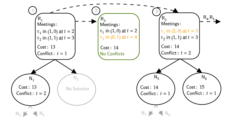
(b) Co-CBS search forest.

Figure 3: Example execution of Co-CBS (3(b)) on the instance depicted in (3(a)). Root and regular nodes are denoted with $R$ and $N$, respectively. The initial root node $R_{1}$ contains the optimal set of meetings, has a cost of $13$ and a conflict at $t=1$. It is expanded to root nodes $R_{2},R_{3}$ (with cost $14$) and split on its first conflict, creating $N_{1},N_{2}$. $N_{2}$ has no solution, thus $N_{1}$ will be chosen next for expansion, creating $N_{3},N_{4}$, both with no solution. In the next iterations, Co-CBS will expand $R_{2}$ (to $R_{4},R_{5},N_{5},N_{6}$), then $N_{5}$, and finally $R_{3}$. Since $R_{3}$ has no conflicts, it will be returned as a feasible optimal solution.

We now continue with an overview of Co-CBS (depicted in Fig. 3 and outlined in Algorithm 1). We then continue with lower-level details.

III-1 Algorithm overview

Co-CBS is a search algorithm based on CBS that considers the cooperative aspect of the problem. More specifically, Co-CBS consists of three levels of search in three different spaces (similar to [19] and [22]): (i) the meetings space, (ii) the conflicts space and (iii) the paths space. The meetings space contains all possible combinations of meetings, one for each task. We’ll refer to the three levels of search as the meetings level, conflicts level and paths level, respectively.

Algorithm 1 Cooperative Conflict-Based Search (Co-CBS)

1:Input: $G,\mathcal{A},\mathcal{B},\mathcal{V}_{0},\mathcal{T}$ $\triangleright$ Co-MAPF problem instance

2:Returns: optimal path for each agent

3:for all $\tau_{i}\in\mathcal{T}$ do $\triangleright$ using Algorithm 2 for each task

4:     $T_{i}\leftarrow compute\_meetings\_table(\tau_{i},\alpha_{i},\beta_{i})$

5:$R.constraints\leftarrow\emptyset$

6:$R.meetings\leftarrow$ get the initial set of optimal meetings

7:$R.root\leftarrow$ True

8:$R.solution\leftarrow plan\_paths()$ $\triangleright$ to and from meetings

9:$R.cost\leftarrow compute\_cost(R.solution)$

10:insert $R$ to OpenRoots

11:while Open $not$ $empty$ or OpenRoots $not$ $empty$ do

12:     $N\leftarrow$ lowest cost node from Open$\cup$OpenRoots

13:     Validate the path in $N$ until a conflict occurs

14:     if $N$ has no conflicts then

15:         return $N.solution$ $\triangleright$ $N$ is goal      

16:     if $N.root\ is\ True$ then

17:         $expand\_root(N)$ $\triangleright$ using Algorithm 3      

18:     $C\leftarrow$ first conflict $\left(a_{i},a_{j},v,t\right)$ in $N$

19:     for all $agent\>a_{i}\>in\>C$ do

20:         $A\leftarrow$ new node

21:         $A.constraints\leftarrow N.constraints+\left(a_{i},v,t\right)$

22:         $A.meetings\leftarrow N.meetings$

23:         $A.root\leftarrow$ False

24:         $A.solution\leftarrow N.solution$

25:         Update $A.solution$ by invoking $plan\_paths(a_{i})$

26:         $A.cost\leftarrow compute\_cost(A.solution)$

27:         Insert $A$ to Open      

Co-CBS simultaneously searches over all possible meetings and for each meeting, over all possible paths. To perform this search in a systematic and efficient manner, we need to consider an ordering of the meetings. Indeed, in Equation 1 we define a meeting’s cost which is dependent both on the meeting’s location and time. To efficiently traverse the set of possible meetings, we introduce the notion of a Meetings Table which stores for each meeting location the currently-best meeting time. As we will see, this table will allow us to iterate over all meetings in a best-first manner.

In contrast to CBS that constructs a single conflicts-tree (CT), Co-CBS creates a forest of CTs, similar to [19]. Each CT starts in a root node and corresponds to a specific set of meetings (a specific meeting for each task). In Co-CBS, each CT node has two additional fields (when compared to CBS): root specifies if the node is a root or a regular node and meetings specifies the current set of meetings (one for each task) which is used during the path-level search.

Co-CBS starts with a single root node, with the optimal set of meetings (see Equation 3), while ignoring possible conflicts between agents. In each iteration, Co-CBS selects a lowest-cost node from the Open list (either a root or regular node), in a best-first approach similar to CBS. Whenever a root node is selected, in addition to splitting the tree due to a conflict, Co-CBS also expands it in the meetings space by generating the next best sets of meetings. Namely, new root nodes are created only on demand. For each expanded node, given its set of meetings and constraints, the paths level computes a solution by planning the different steps a task solution is composed of (Section II-B).

Algorithm 2 Compute Meetings Table

1:Input: A Task $\tau_{i}$ and two assigned agents

2:Returns: $T_{i}$, the meetings table for task $\tau_{i}$

3:Compute $d\left(\mathcal{V}_{0}\left(\alpha_{i}\right),s_{i}\right)$ $\triangleright$ initiator start to task start

4:Compute $d\left(s_{i},v\right),\forall v\in V$ $\triangleright$ task start to all

5:Compute $d\left(\mathcal{V}_{0}\left(\beta_{i}\right),v\right),\forall v\in V$ $\triangleright$ executor start to all

6:Compute $d\left(v,g_{i}\right),\forall v\in V$ $\triangleright$ task goal to all

7:for all $v\in V$ do

8:     Calculate $t_{i}^{*}\left(v\right)$ $\triangleright$ earliest meeting time in $v$

9:     Calculate $T_{i}\left(v\right)$ $\triangleright$ task cost with meeting at $v$

10:     Store $\left(v,t_{i}^{*}\left(v\right),T_{i}\left(v\right)\right)$ in table

Algorithm 3 Expand root

1:Input: Meetings tables of all tasks, a root node $P$

2:for all $\tau_{i}\in\mathcal{T}$ do $\triangleright$ loop over all tasks

3:     $R=$ new node

4:     $R.constraints=\emptyset$

5:     $R.meetings=P.meetings$

6:     $R.meetings[\tau_{i}]=get\_next\_meeting(T_{i})$

7:     $R.root$ = True

8:     Update $R.solution$ by invoking $plan\_paths(\alpha_{i},\beta_{i})$

9:     $R.cost=compute\_cost(R.solution)$

10:     insert $R$ to OpenRoots

III-2 Computing the Meetings Table

We denote the cost of a meeting $m_{i}=\left(v_{i}^{m},t_{i}^{m}\right)$ as $C_{i}(v_{i}^{m},t_{i}^{m})$. $C_{i}$ is given for the SOC objective, by

$$C_{i}(v,t)=\left\{\begin{array}[]{cc}2\cdot t+d\left(v,g_{i}\right),&t\geq t_{i}^{*}\left(v\right)\\ \infty,&\text{otherwise}\end{array}\right.,$$ (1)

where $t_{i}^{*}\left(v\right)$ is the earliest possible meeting time at $v$ for task $\tau_{i}$, i.e., the earliest time both assigned agents can arrive at $v$. Specifically, $t_{i}^{*}\left(v\right)$ is defined as

$$\begin{split}t_{i}^{*}\left(v\right)=\max\left\{d\left(\mathcal{V}_{0}\left(\alpha_{i}\right),s_{i}\right)+d\left(s_{i},v\right),\right.\\ \left.d\left(\mathcal{V}_{0}\left(\beta_{i}\right),v\right)\right\}\end{split},$$ (2)

where $d(u,v)$ is the length of the single-agent shortest path from $u$ to $v$. If ${d(u,v)=\infty}$, no such path exists.

The first step of Co-CBS is to compute $T_{i}$, the meetings table for each task $\tau_{i}$ (lines 3-4). The meetings table is a function ${T_{i}:V\rightarrow\mathbb{R}\cup\left\{\infty\right\}}$ that returns for each vertex ${v\in V}$ the cost for completing task $\tau_{i}$ with a meeting in $v$ at the earliest possible time. ${T_{i}\left(v\right)}$ is initialized for each ${v\in V}$ with ${T_{i}\left(v\right)=C_{i}(v,t_{i}^{*}\left(v\right))}$. Each meetings table is stored as a heap which allows for $insert$, $update$ and $getMin$ operations in $\mathcal{O}(\log\left|V\right|)$. These operations are used during the root node expansion which will be described shortly.

We compute $T_{i}\left(v\right)$ for all $v\in V$ in polynomial time using A* and Dijkstra’s algorithm as described in Algorithm 2. Computing the meetings table for each task $\tau_{i}$ requires finding paths from every node $v\in V$ to the agents’ start locations, as well as tasks’ start and goal locations. Given the meeting tables, we can check if the given problem instance is well-formed (see Definition II.1). More specifically, it is well-formed iff for every meetings table $T_{i}$ there exists a vertex $v\in V\setminus V_{ep}$ such that $T_{i}\left(v\right)<\infty$.

(a) Example instance with two tasks: $\alpha_{1}$ and $\beta_{1}$ execute $\tau_{1}$ from $s_{1}$ to $g_{1}$ and $\alpha_{2}$ and $\beta_{2}$ execute $\tau_{2}$ from $s_{2}$ to $g_{2}$.

III-3 Root initialization

We define the cost of a set of meetings ${\mathcal{M}=\left\{m_{1},\dots,m_{k}\right\}}$ as follows: ${C\left(\mathcal{M}\right)=\sum_{i=1}^{k}{C_{i}\left(v_{i}^{m},t_{i}^{m}\right)}}$. $\mathcal{M}^{*}$ is an optimal set of meetings that minimizes the problem objective while ignoring possible conflicts between agents. Namely,

$$\mathcal{M}^{*}\in\operatorname*{arg\,min}_{\mathcal{M}}{C\left(\mathcal{M}\right)}.$$ (3)

Co-CBS’s search starts with creating the initial CT root node with an empty set of constraints, and an optimal set of meetings ${\mathcal{M}^{*}}$, by choosing a lowest-cost meeting for each task from the meeting tables (lines 5-7). Given $\mathcal{M}^{*}$, the paths level is called to compute individual paths for each agent (line 8). This is similar to CBS, except that in the path-level search we plan for each task $\tau_{i}$ in parts: (i) for ${\alpha_{i}}$ from ${\mathcal{V}_{0}\left(\alpha_{i}\right)}$ to $s_{i}$, and then from $s_{i}$ to ${v_{i}^{m}}$ at time $t_{i}^{m}$, and (ii) for ${\beta_{i}}$ from ${\mathcal{V}_{0}\left(\beta_{i}\right)}$ to ${v_{i}^{m}}$ at time ${t_{i}^{m}}$ and then to $g_{i}$. Note that when planning for a meeting, we should consider both the meeting location and time. The initial CT root node cost is computed and it is inserted to the Open list (lines 9-10).

III-4 Selecting a node for expansion

As long as there are nodes in the Open list (line 11), we follow CBS’s best-first search approach and select a node with a lowest cost (line 12). If the Open list contains both root and regular nodes with the same lowest cost, Co-CBS chooses to expand a regular node (to perform this in practice, Co-CBS keeps root and regular nodes in two separate Open lists).

III-5 Expanding a root node

After selecting a lowest-cost node $N$ from the Open list, Co-CBS checks for conflicts in its solution (line 13). If none are found, $N.solution$ is returned as the optimal solution (lines 14-15). Otherwise, if $N$ is a root node, it is expanded to get its successors in the meetings space (lines 16-17). The process of expanding a root node is described in Algorithm 3. Given the current set of meetings (in the expanded root node) ${\mathcal{M}=\left\{m_{1},\dots,m_{k}\right\}}$, Co-CBS generates up to $k$ new sets of meetings, one for each task. This is done in a non-decreasing manner, by replacing one meeting $m_{i}\in\mathcal{M}$ at a time, an idea similar to the Increasing Cost Tree Search (ICTS) [23] algorithm, thus creating $k$ new root nodes.

To get the next-best meeting for task $\tau_{i}$, we have to search both for different locations and time steps in the meetings space. The meetings table $T_{i}$ of $\tau_{i}$ initially consists of meetings at each possible location, at the earliest time possible. Each time Co-CBS invokes the get-next-meeting procedure for $\tau_{i}$ (line 6 in Algorithm 3), it returns the lowest-cost meeting ${m_{i}=\left(v_{i}^{m},t_{i}^{m}\right)}$ from $T_{i}$. The table is then updated so that it holds the next lowest-cost meeting. This is done by updating ${T_{i}\left(v_{i}^{m}\right)=C_{i}\left(v_{i}^{m},t_{i}^{m}+1\right)}$. Namely, updating the cost of meeting at ${v_{i}^{m}}$, but at time ${t_{i}^{m}+1}$ rather than ${t_{i}^{m}}$. The next time the get-next-meeting procedure is invoked, the next best meeting will be returned by the table.

Subsequently, a new path is planned for the pair of agents whose meeting changed, the new CT node cost is computed and it is inserted into the Open list.

III-6 Resolving a conflict

The last part of the algorithm is almost identical to CBS: when expanding a node $N$ (either root or regular) Co-CBS splits its CT and creates a regular node for each agent by the first conflict found (lines 18-19). These nodes has the same set of meetings as $N$ (line 22).

IV Theoretical Analysis

IV-A Co-CBS Completeness

We restrict our discussion to well-formed Co-MAPF instances. We guarantee completeness of Co-CBS on well-formed instances using Claim II.1, which states that if the instance is not well-formed we can identify it by running a polynomial-time test procedure before executing Co-CBS.

Theorem IV.1

Co-CBS will return a solution for any well-formed Co-MAPF instance.

Proof Sketch: By Lemma II.1 we know that there exists a solution. Denote the set of meetings which forms the solution by ${\mathcal{M}=\left\{\left(v_{1}^{m},t_{1}^{m}\right),\left(v_{2}^{m},t_{2}^{m}\right),\dots,\left(v_{k}^{m},t_{k}^{m}\right)\right\}}$. Co-CBS’s meetings level preforms a systematic best-first search across the meetings space, thus, will eventually create a root node, denoted by $R_{\mathcal{M}}$, whose set of meetings is $\mathcal{M}$. There exists a feasible solution such that each pair of agents ${\left(\alpha_{i},\beta_{i}\right)}$ meet at ${\left(v_{i}^{m},t_{i}^{m}\right)}$. By the completeness of CBS it is guaranteed that the search from the CT root node ${R_{\mathcal{M}}}$ will eventually find the solution.  ∎

IV-B Co-CBS Optimality

We again restrict the discussion to well-formed instances. By Theorem IV.1 we are guaranteed that Co-CBS solves every well-formed Co-MAPF instance. We show that it returns an optimal solution for the SOC objective function.

Lemma IV.2

Let $\mathcal{M}$ be a set of meetings with ${C\left(\mathcal{M}\right)=c}$ and let $N$ be a CT node with cost larger than $c$. Co-CBS will generate a root node corresponding to $\mathcal{M}$ before expanding $N$.

Proof Sketch: Assume that there exists a set of meetings $\mathcal{M}$ s.t. ${C(\mathcal{M})=c}$, that hasn’t been generated yet. Assume by contradiction that Co-CBS expands a node $N$ that has a solution with cost ${c^{\prime}>c}$. By definition, the first set of meetings $\mathcal{M}_{0}$ that is generated (line 6 in Algorithm 1) induces a solution which minimizes the SOC objective function. In particular, this implies that the cost of completing all tasks in the (possibly infeasible) solution induced by ${\mathcal{M}_{0}}$ is less than or equal to $c$. Similarly, the cost of completing all tasks in the solution induced by ${\mathcal{M}}$ is less than or equal to $c$. Therefore, there exists a sequence of meeting placements that may be generated during the meetings-level search, from ${\mathcal{M}_{0}}$ to ${\mathcal{M}}$, such that the cost of the meetings sets in the sequence would remain smaller or equal to $c$ at all time, i.e., each set of meetings $\mathcal{M}^{\prime}$ in this sequence holds ${C(\mathcal{M}^{\prime})\leq c}$. The way the meetings-level search works ensures that there must be at least one root node in the Open list consisting of one of these meeting sets. Therefore, there exists a root node that hasn’t been expanded yet in the Open list with a cost smaller than $c^{\prime}$, in contradiction to the best-first search approach which chose node $N$ with a larger cost for expansion.  ∎

Theorem IV.3

Co-CBS returns an optimal solution for any well-formed Co-MAPF instance.

Proof Sketch: Assume that there exists an optimal solution with some cost $c^{*}$. Co-CBS performs a CBS-like search on each generated CT, namely, it searches through a forest of conflict trees. By Lemma IV.2 we get that the cost of each expanded root node of each CT constitutes a lower-bound on $c^{*}$. From the optimality guarantees of CBS, we get that any node expanded in each of those CTs (i.e., regular nodes) is also a lower bound on $c^{*}$. Due to Co-CBS’s best-first approach, it won’t expand a node with a cost larger than $c^{*}$ before completing a search through all possible CT nodes with cost $c^{*}$ (by expanding neither a root node nor a regular one). Since there exists a solution with such cost, and the number of possible solutions with a specific cost is finite, Co-CBS will eventually expand a node with an optimal and feasible solution and return it.  ∎

IV-C Co-CBS Runtime Analysis

Co-CBS is an extension of CBS which adds a level that searches in the meeting space. The size of the meeting space is ${\mathcal{O}((|V|\cdot c^{*})^{k})}$. In the worst case, Co-CBS would generate all possible meetings and perform a CBS search for each set of meetings (up-to cost $c^{*}$). It may result in a number of expanded nodes relative to the number of meeting points, times the number of nodes expanded by CBS [18, 24].

In practice, in our empirical evaluation (Section VI) we observe that the number of generated meeting sets is typically small, especially for large or sparse environments (see Fig. 5(a)). This means that the number of full CBS searches (one for each meetings set) is usually small. However, in scenarios with many conflicts, a large number of root nodes (and, meeting sets) are created. This causes an increase in run time which is exponential in the number of tasks.

V Co-CBS Improvements

In the previous section, we introduced the basic version of Co-CBS for solving the Co-MAPF problem. Co-CBS creates a forest of conflict trees and runs CBS on each tree. Thus, we can apply previously-suggested CBS improvements to Co-CBS. One such improvement that has been shown to significantly decrease CBS’s run-time is prioritizing conflicts (PC) [25]. In this section we present in details the application of PC to Co-CBS. More CBS improvements are discussed in Section VII. In addition, we introduce a unique improvement for Co-CBS called Lazy Expansion (LE), which exploits special characteristics of root nodes. Both improvements keep Co-CBS optimal, while introducing a significant improvement in run time, as shown empirically in Section VI.

V-A Prioritizing Conflicts (PC) for Co-CBS

The Improved CBS (ICBS) algorithm [25] introduced an enhancement to CBS by defining rules dictating how to split the CT. In particular, conflicts are divided into three types: cardinal, semi-cardinal and non-cardinal. Cardinal conflicts always cause an increase in the solution cost, therefore ICBS chooses to split cardinal conflicts first. Cardinal conflicts are identified by examining the width of a multi-value decision diagram (MDD) [23], which is constructed for each low-level path found. The MDD is a directed a-cyclic graph which compactly stores all possible paths of a given cost $c$ for a given agent, from its start vertex to its goal vertex. An MDD of cost $c$ consists of $c$ layers, corresponding to $c$ time steps.

Applying PC to Co-CBS is not straightforward, since an MDD stores paths from a start vertex to a goal vertex, while in Co-MAPF paths are constrained to ensure cooperation between agents. More specifically, in our Co-MAPF setting, each agent has an intermediate goal, i.e., the task start location, or the meeting location (at a specific time). We therefore need to modify the way an MDD is constructed, and indeed we suggest a method for efficiently doing so for both agents.

For the initiator agent, we must ensure it passes through the task’s start location. In other words, we need to prune MDD nodes that are not part of any of the agent’s paths which pass the task’s start location. We refer to such nodes as invalid nodes. Constructing an MDD efficiently is done using two breadth-first searches–one forward and one backward (start to goal and vise versa) [23]. In order to efficiently prune invalid nodes, we follow the following procedure: during the forward search, we mark MDD nodes corresponding to the task start location and all their descendants as valid_forward. Similarly, during the backward search, we mark these nodes and all their ancestors as valid_backward. Finally, all MDD nodes that are not marked with either flags are pruned.

For the executor agent, constructing the MDD requires only slight changes. We need to constrain the agent to be at the meeting’s location at the meeting’s time. We simply do it by eliminating all other nodes from the MDD layer corresponds to the meeting time during the forward pass in the MDD construction.

V-B Lazy Expansion (LE) of root nodes

Co-CBS searches the meetings space by creating root nodes, each corresponding to a unique set of meetings. Note that since no constraints are imposed on paths of root nodes, their cost is given as an aggregation of their meeting costs. Furthermore, meeting costs are computed a-priori during the construction of meeting tables (see Section III). This means that when a root node is expanded, and new root nodes are created, they can immediately be inserted into the Open list without computing their low-level paths. The low-level paths will be computed only when these root nodes are extracted from the Open list. We term this Lazy Expansion (LE).

Each time a root node is expanded, it creates $k$ new root nodes by replacing the meeting of each of the tasks. We emphasize that while generating those nodes is mandatory in order to guarantee optimality, most of them won’t be expanded. Thus, the run-time saved by LE can be significant.

VI Experimental Evaluation

Co-CBS solves the newly introduced Co-MAPF problem. To the best of our knowledge, there does not exist an off-the-shelf optimal solver for MAPF problems involving cooperative behavior. Suggesting a centralized A*-based implementation for solving the Co-MAPF problem is challenging due to constraints imposed on low-level paths to achieve cooperation. Such approach would require to perform a search in the meetings space, resulting in an exponentially-large state space. Moreover, an attempt to solve Co-MAPF using such implementation would yield similar results as solving classical MAPF problem using A* [18], due to their similar search approach and conflict-resolution mechanism. Thus, we restrict our empirical evaluation to the algorithms presented in this paper.

To measure the quality of Co-CBS, we present the results of an empirical evaluation performed on standard MAPF benchmarks [2, 26] showing the performance of the basic version of Co-CBS, as well as the two suggested improvements (see Section V). Co-CBS is implemented in C++ and is based on the implementation of Li et al. [27]. All simulations were performed on an Intel Xeon Platinum 8000 @ 3.1Ghz machine with 32.0 GB RAM.

VI-A Benchmarks and setup

We evaluated Co-CBS on several 2D grid-based benchmarks. Specifically, we tested Co-CBS on different types of maps—a dense game map (DAO, den312d), random map (random-32-32-20), a large warehouse (warehouse-10-20-10-2-1) and a custom small warehouse ($57\times 27$). We ran 25 random queries for each benchmark for the SOC objective with the number of tasks ranging from $6$ tasks ($12$ agents) to $22$ tasks (44 agents) and with a timeout of two minutes. On each benchmark, we compare the performance of three different variances of Co-CBS: (i) basic Co-CBS, (ii) Co-CBS with prioritizing conflicts (PC), and (iii) Co-CBS with PC and lazy expansion (LE) of root nodes. As opposed to the classical MAPF, where each agent is provided with start and goal locations, in Co-MAPF, a task’s start and goal need to be provided (instead of explicitly providing an agents’ goal). Thus, we defined the tasks in each scenario as follows, based on the original benchmark scenario: for each pair of agents, one set of start and goal locations is used for the task, and the other set is used for the agents’ start locations.

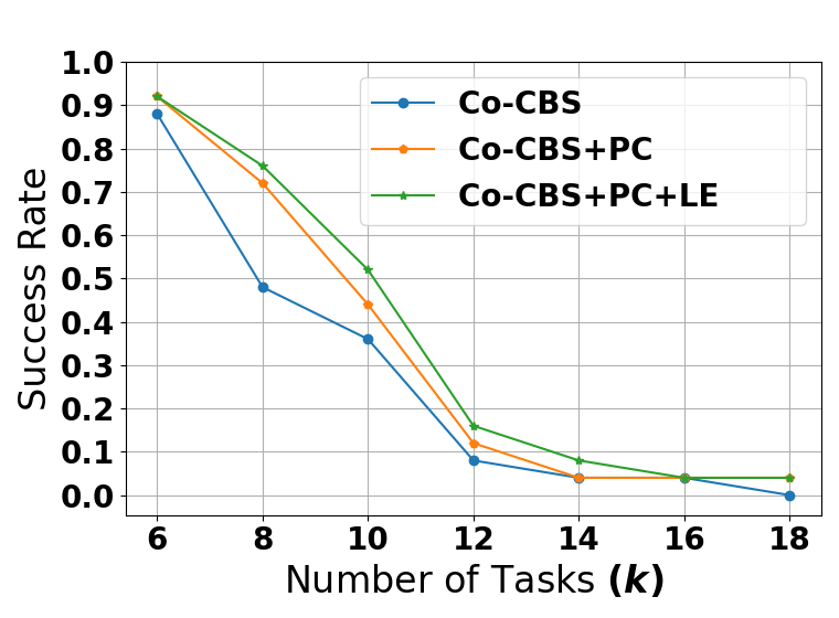
(a) den312d

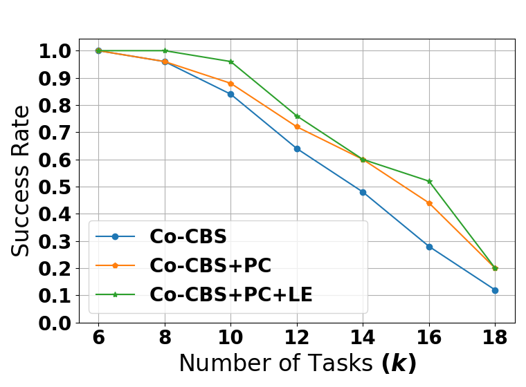
(b) random-32-32-20

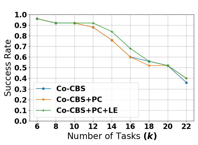
(c) warehouse-10-20-10-2-1

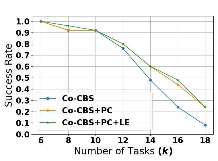
(d) warehouse-57-27

Figure 4: Success rates.

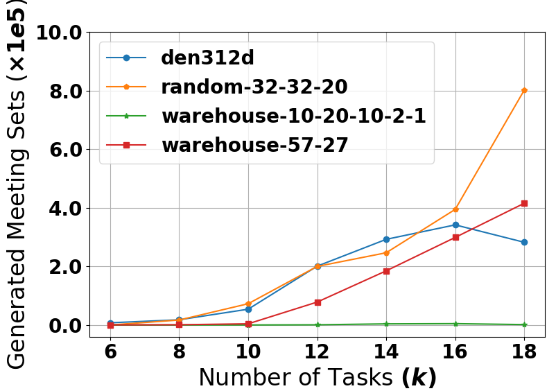
(a)

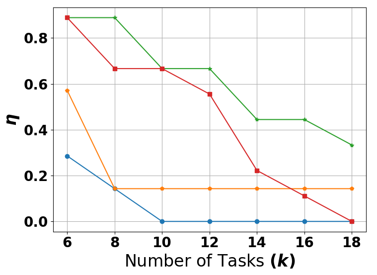
(b)

Figure 5: (5(a)) Number of generated sets of meetings. (5(b)) Ratio $\eta$ between the number of instances solved using the first set of meetings, and the total number of instances.

VI-B Results

We first examine the algorithm’s success rate (i.e., the ratio of solved instances within the time limit) for all benchmarks. Figures 4 shows the success rates of Co-CBS on all maps. Co-CBS successfully solves more than $80\%$ of the instances (excluding the den312d benchmark) with ten tasks. The success rate sharply drops below $20\%$ for twelve tasks or more on the dense den312d map. Using PC improves the basic Co-CBS in all cases, achieving up to $30\%$ increase in the success rate. Furthermore, adding LE on top of PC further improves the performance in most cases, and never degrades the performance. This is especially notable with a large number of tasks, where many root nodes are created.

Fig. 5(a) shows the average number of generated meeting sets. Fig. 5(b) shows the ratio $\eta$ between the number of instances where the first set of meetings is used to obtain the solution and the total number of instances. Both warehouse environments are typically sparser, causing fewer conflicts between agents. Thus, a feasible solution is usually quickly found using the first set of meetings. This is especially true in the large warehouse, namely when $\eta$ is close to one. The search in this case is equivalent to running CBS with the first set of meetings. For the same reason, PC does not improve the performance in this environment. Applying LE as well, however, does manage to improve the success rate for the majority of tasks. In other environments, on the other hand, maps are smaller and denser, and most solutions are not obtained using the first generated set of meetings. A more exhaustive meeting-space search is therefore required to find an optimal solution, as shown in Fig. 5(a).

VII Discussion and Future Work

In this paper, we introduced the Cooperative Multi-Agent Path Finding (Co-MAPF) problem, an extension to classical MAPF that incorporates cooperative behavior. We introduced Co-CBS, a three-level search algorithm that optimally solves Co-MAPF instances, as well as two improvements, Prioritizing Conflict (PC) and Lazy Expansion (LE).

In this section, we provide a comprehensive discussion regarding the suggested model and algorithm. Specifically, we discuss further possible improvements that can be applied to Co-CBS and suggest possible extensions to the Co-MAPF model. We argue that Co-CBS forms a basic framework that may serve as a starting point for future extensions.

VII-A Co-CBS’s Extensions and Improvements

VII-A1 Information reusing between conflict trees

Co-CBS expands root nodes by only changing one meeting in the newly-created node. Moreover, the next selected meeting is usually very close to the current meeting, both in location and time. This implies that Co-CBS searches over multiple trees that potentially have very similar solutions. We may exploit this for more efficient computation.

VII-A2 Meetings-level search

Co-CBS uses a simple-yet-effective method for finding an optimal meeting for each task. For large problem instances, this method may become memory and run-time expensive, due to the maintenance of large meeting tables. We may consider incorporating an algorithm such as the recently-proposed MM* algorithm [28], for the Multi-Agent Meeting problem. Furthermore, we may couple meetings and paths planning, and handle conflicts during the search for a meeting. This may be advantageous as meetings and conflicts may be tightly coupled.

VII-A3 Existing CBS improvements

In addition to the PC improvement presented in Section V, more CBS improvements exist. Some of these include adding heuristics [29], disjoint splitting [30], bypassing a conflict [31], symmetry breaking [32] and exploiting similarities between nodes in a single conflict tree [33]. We can also apply variants of CBS [34] that compute (bounded) sub-optimal solutions to Co-CBS.

VII-B Extensions to the Co-MAPF Framework

VII-B1 Number and types of collaborating agents

A rather straightforward generalization of Co-MAPF is to require more than two agents to collaborate on a task. The problem introduced in Section I motivates this extension: several grasp units may pickup several items for a single transfer unit. Co-CBS can solve this problem with a few minor changes. However, if the number of agents per task isn’t fixed, additional work is required. Moreover, we may consider agents with different traversal capabilities (e.g., different velocities [6]), by possibly changing the single-agent planner.

VII-B2 Other forms of cooperative interaction

We introduced a definition for the Co-MAPF problem, where interaction between agents is expressed via meetings between two types of agents. While this interaction is very intuitive, more forms of cooperative interaction can be modeled (for example, temporal constraints). We may generalize the formulation to include a finite set of possible agent types, and define more complex tasks where each agent type has its dedicated role.

The framework provided by Co-CBS might allow to address such general definitions by only adjusting the cooperation-level search (the meetings level in our case). Any cooperative planning, which results in inducing goals for an agent, can be easily plugged in into Co-CBS.

VII-B3 Task assignment and lifelong planning

In this problem we assume cooperative tasks are pre-assigned to collaborating agents. However, optimizing the task assignment as well may significantly affect solution quality (as in classical MAPF). This is extremely relevant for lifelong-planning problems, where agents have to attend to a stream of incoming tasks. Generalizing the Co-MAPF framework in this direction will advance it even further towards more real-world problems, but introduce significant challenges as well.

References

- [1] A. Torreño, E. Onaindia, A. Komenda, and M. Stolba, “Cooperative multi-agent planning: A survey,” Computing Research Repository (CoRR), vol. abs/1711.09057, 2017.
- [2] R. Stern, N. R. Sturtevant, A. Felner, S. Koenig, H. Ma, T. T. Walker, J. Li, D. Atzmon, L. Cohen, T. K. S. Kumar, R. Barták, and E. Boyarski, “Multi-agent pathfinding: Definitions, variants, and benchmarks,” in Int. Symp. on Combinatorial Search (SOCS), 2019, pp. 151–159.
- [3] P. R. Wurman, R. D’Andrea, and M. Mountz, “Coordinating hundreds of cooperative, autonomous vehicles in warehouses,” Artificial Intelligence, vol. 29, no. 1, pp. 9–20, 2008.
- [4] K. Dresner and P. Stone, “A multiagent approach to autonomous intersection management,” Journal of Artificial Intelligence Research (JAIR), vol. 31, pp. 591–656, 2008.
- [5] J. Švancara, M. Vlk, R. Stern, D. Atzmon, and R. Barták, “Online multi-agent pathfinding,” in AAAI Conf. on Artificial Intelligence, vol. 33, 2019, pp. 7732–7739.
- [6] W. Hönig, T. K. S. Kumar, L. Cohen, H. Ma, H. Xu, N. Ayanian, and S. Koenig, “Multi-agent path finding with kinematic constraints,” in Int. Conf. Automated Planning and Scheduling (ICAPS). AAAI Press, 2016, pp. 477–485.
- [7] H. Ma, S. Koenig, N. Ayanian, L. Cohen, W. Hönig, T. K. S. Kumar, T. Uras, H. Xu, C. A. Tovey, and G. Sharon, “Overview: Generalizations of multi-agent path finding to real-world scenarios,” Computing Research Repository (CoRR), vol. abs/1702.05515, 2017.
- [8] A. Felner, R. Stern, S. E. Shimony, E. Boyarski, M. Goldenberg, G. Sharon, N. R. Sturtevant, G. Wagner, and P. Surynek, “Search-based optimal solvers for the multi-agent pathfinding problem: Summary and challenges,” in Int. Symp. on Combinatorial Search (SOCS), 2017, pp. 29–37.
- [9] O. Salzman and R. Stern, “Research challenges and opportunities in multi-agent path finding and multi-agent pickup and delivery problems,” in Int. Conf. on Autonomous Agents and MultiAgent Systems (AAMAS), 2020, pp. 1711–1715.
- [10] H. Ma, J. Li, T. K. S. Kumar, and S. Koenig, “Lifelong multi-agent path finding for online pickup and delivery tasks,” in Int. Conf. on Autonomous Agents and MultiAgent Systems (AAMAS), 2017, pp. 837–845.
- [11] M. Liu, H. Ma, J. Li, and S. Koenig, “Task and path planning for multi-agent pickup and delivery,” in Int. Conf. on Autonomous Agents and MultiAgent Systems (AAMAS), 2019, pp. 1152–1160.
- [12] H. Ma, C. A. Tovey, G. Sharon, T. K. S. Kumar, and S. Koenig, “Multi-agent path finding with payload transfers and the package-exchange robot-routing problem,” in AAAI Conf. on Artificial Intelligence, 2016, pp. 3166–3173.
- [13] D. Atzmon, Y. Zax, E. Kivity, L. Avitan, J. Morag, and A. Felner, “Generalizing multi-agent path finding for heterogeneous agents,” in Int. Symp. on Combinatorial Search (SOCS), 2020, pp. 101–105.
- [14] N. Correll, K. E. Bekris, D. Berenson, O. Brock, A. Causo, K. Hauser, K. Okada, A. Rodriguez, J. M. Romano, and P. R. Wurman, “Analysis and observations from the first Amazon picking challenge,” IEEE Transactions on Automation Science and Engineering, vol. 15, no. 1, pp. 172–188, 2016.
- [15] R. Shome, “Roadmaps for robot motion planning with groups of robots,” Current Robotics Reports, pp. 1–10, 2021.
- [16] C. C. Murray and R. Raj, “The multiple flying sidekicks traveling salesman problem: Parcel delivery with multiple drones,” Transportation Research Part C: Emerging Technologies, vol. 110, pp. 368–398, 2020.
- [17] S. Choudhury, K. Solovey, M. J. Kochenderfer, and M. Pavone, “Efficient large-scale multi-drone delivery using transit networks,” in IEEE Int. Conf. Robotics and Automation (ICRA), 2020, pp. 4543–4550.
- [18] G. Sharon, R. Stern, A. Felner, and N. R. Sturtevant, “Conflict-based search for optimal multi-agent pathfinding,” Artificial Intelligence, vol. 219, pp. 40–66, 2015.
- [19] W. Hönig, S. Kiesel, A. Tinka, J. W. Durham, and N. Ayanian, “Conflict-based search with optimal task assignment,” in Int. Conf. on Autonomous Agents and MultiAgent Systems (AAMAS), 2018, pp. 757–765.
- [20] M. Cáp, J. Vokrínek, and A. Kleiner, “Complete decentralized method for on-line multi-robot trajectory planning in well-formed infrastructures,” in Int. Conf. Automated Planning and Scheduling (ICAPS), 2015, pp. 324–332.
- [21] J. Yu and D. Rus, “Pebble motion on graphs with rotations: Efficient feasibility tests and planning algorithms,” in Workshop on the Algorithmic Foundations of Robotics (WAFR), ser. Springer Tracts in Advanced Robotics, vol. 107, 2014, pp. 729–746.
- [22] P. Surynek, “Multi-goal multi-agent path finding via decoupled and integrated goal vertex ordering,” Computing Research Repository (CoRR), vol. abs/2009.05161, 2020.
- [23] G. Sharon, R. Stern, M. Goldenberg, and A. Felner, “The increasing cost tree search for optimal multi-agent pathfinding,” Artificial Intelligence, vol. 195, pp. 470–495, 2013.
- [24] O. Gordon, Y. Filmus, and O. Salzman, “Revisiting the complexity analysis of conflict-based search: New computational techniques and improved bounds,” Computing Research Repository (CoRR), vol. abs/2104.08759, 2021.
- [25] E. Boyarski, A. Felner, R. Stern, G. Sharon, D. Tolpin, O. Betzalel, and S. E. Shimony, “ICBS: improved conflict-based search algorithm for multi-agent pathfinding,” in Int. Joint Conf. on Artificial Intelligence (IJCAI), 2015, pp. 740–746.
- [26] N. Sturtevant, “Benchmarks for grid-based pathfinding,” Transactions on Computational Intelligence and AI in Games, vol. 4, no. 2, pp. 144 – 148, 2012. [Online]. Available: http://web.cs.du.edu/ sturtevant/papers/benchmarks.pdf
- [27] J. Li, D. Harabor, P. J. Stuckey, and S. Koenig, “Pairwise symmetry reasoning for multi-agent path finding search,” Computing Research Repository (CoRR), vol. abs/2103.07116, 2021.
- [28] D. Atzmon, J. Li, A. Felner, E. Nachmani, S. S. Shperberg, N. Sturtevant, and S. Koenig, “Multi-directional heuristic search,” in Int. Joint Conf. on Artificial Intelligence (IJCAI), 2020, pp. 4062–4068.
- [29] A. Felner, J. Li, E. Boyarski, H. Ma, L. Cohen, T. K. S. Kumar, and S. Koenig, “Adding heuristics to conflict-based search for multi-agent path finding,” in Int. Conf. Automated Planning and Scheduling (ICAPS), 2018, pp. 83–87.
- [30] J. Li, D. Harabor, P. J. Stuckey, H. Ma, and S. Koenig, “Disjoint splitting for multi-agent path finding with conflict-based search,” in Int. Conf. Automated Planning and Scheduling (ICAPS), 2019, pp. 279–283.
- [31] E. Boyarski, A. Felner, G. Sharon, and R. Stern, “Don’t split, try to work it out: Bypassing conflicts in multi-agent pathfinding,” in Int. Conf. Automated Planning and Scheduling (ICAPS), 2015, pp. 47–51.
- [32] J. Li, G. Gange, D. Harabor, P. J. Stuckey, H. Ma, and S. Koenig, “New techniques for pairwise symmetry breaking in multi-agent path finding,” in Int. Conf. Automated Planning and Scheduling (ICAPS), 2020, pp. 193–201.
- [33] E. Boyarski, A. Felner, D. Harabor, P. J. Stuckey, L. Cohen, J. Li, and S. Koenig, “Iterative-deepening conflict-based search,” in Int. Joint Conf. on Artificial Intelligence (IJCAI), 2020, pp. 4084–4090.
- [34] M. Barer, G. Sharon, R. Stern, and A. Felner, “Suboptimal variants of the conflict-based search algorithm for the multi-agent pathfinding problem,” in Int. Symp. on Combinatorial Search (SOCS), 2014.