FBI-Denoiser: Fast Blind Image Denoiser for Poisson-Gaussian Noise

Abstract

We consider the challenging blind denoising problem for Poisson-Gaussian noise, in which no additional information about clean images or noise level parameters is available. Particularly, when only “single” noisy images are available for training a denoiser, the denoising performance of existing methods was not satisfactory. Recently, the blind pixelwise affine image denoiser (BP-AIDE) was proposed and significantly improved the performance in the above setting, to the extent that it is competitive with denoisers which utilized additional information. However, BP-AIDE seriously suffered from slow inference time due to the inefficiency of noise level estimation procedure and that of the blind-spot network (BSN) architecture it used. To that end, we propose Fast Blind Image Denoiser (FBI-Denoiser) for Poisson-Gaussian noise, which consists of two neural network models; 1) PGE-Net that estimates Poisson-Gaussian noise parameters $2000$ times faster than the conventional methods and 2) FBI-Net that realizes a much more efficient BSN for pixelwise affine denoiser in terms of the number of parameters and inference speed. Consequently, we show that our FBI-Denoiser blindly trained solely based on single noisy images can achieve the state-of-the-art performance on several real-world noisy image benchmark datasets with much faster inference time ($\times 10$), compared to BP-AIDE. The official code of our method is available at https://github.com/csm9493/FBI-Denoiser.

1 Introduction

Convolutional neural network (CNN)-based denoisers achieved impressive state-of-the-art denoising performances mainly by utilizing the supervised learning approach based on collecting many clean and noisy image pairs. The performance gain was first shown in the additive white Gaussian noise setting [47, 42, 48, 26, 36, 14], then the approach was extended also to the Poisson-Gaussian noise setting, which better models the real-world source-dependent noise. It was demonstrated that the gain was attained not only with respect to the quantitative metrics, e.g., PSNR or SSIM [44], on the real-world noise benchmarks such as DND [35], SIDD [3] and FMD [49], but also with respect to the inference time for denoising (using GPUs), compared to the more conventional prior- or optimization-based methods [17, 21].

Despite above promising achievements, the plain supervised learning approach has a critical drawback in a more practical, real-world setting, since the availability of the enough number of the clean-noisy image pairs for training is sometimes a luxury that cannot be simply assumed. For example, in medical imaging (CT or MRI), obtaining the underlying clean image for a noisy image becomes extremely time-consuming and expensive. In order to overcome this drawback, several attempts have been made in recent years. The first approach is to utilize unpaired clean images and generate synthetic noisy images to again carry on the supervised training with the generated pairs. For example, in [7, 46], based on in-camera signal processing (ISP) pipeline and specific Poisson-Gaussian noise parameters, they generated synthetic noisy sRGB or rawRGB images from clean sRGB images. Another examples can be found in [45, 16], in which they learned a model to generate noise present in the given noisy images, then used that model to corrupt the clean images to build paired supervised training set. While these approaches were shown to achieve good performance for some specific settings, they either lack generalities or have limited performance for real-world noisy image denoising. The second recent approach to remove the requirement of clean-noisy pairs is to train a denoiser solely based on noisy images [25, 23, 6, 24, 38, 34, 13, 41]. However, those methods also had their own limitations, such as requiring pairs of independently realized noisy images for the same clean source [25, 50], poor performance on benchmark datasets [23, 6], large inference time due to requiring many number of samplings [38], and limited or no experiment on real-world noise setting [24, 34, 41, 50, 13].

Recently, BP-AIDE [10], which extends the framework of [12, 11], was proposed as another attempt to lift the requirement of clean images. Namely, the scheme made a unique combination of Generalized Anscombe Transformation (GAT) [5], Poisson-Gaussian noise estimation [28, 20], and an unbiased estimator of MSE for pixelwise affine denoisers proposed in [11] in order to train a blind denoiser for Poisson-Gaussian noise solely on single noisy images with no additional information. The method achieved the state-of-the-art performance on several benchmarks for real-world noise [49, 3, 35] compared to the methods [23, 17] that operate in the identical setting. However, BP-AIDE had one critical limitation; it suffers from the slow inference time due to the following two reasons. First, for every given noisy image, BP-AIDE must separately carry out the Poisson-Gaussian noise parameter estimation, which usually takes a couple of seconds for moderately sized images. Second, the method simply utilizes the so-called blind-spot network (BSN) architecture proposed in [12] as a denoiser, but the corresponding structure is quite complex and requires large GPU memory, leading to a slow inference time.

To tackle above limitation, we make two significant improvements on BP-AIDE and propose Fast Blind Image Denoiser (FBI-Denoiser). Firstly, we propose PGE (Poisson-Gaussian Estimation)-Net, which learns to estimate the Poisson-Gaussian noise parameters solely from noisy images by converting GAT and Gaussian noise estimation steps to tensor operations and by proposing a novel loss function. Secondly, we devise FBI-Net, a new compact fully convolutional BSN, which performs almost the same as the network in [12] but significantly reduces the inference time. The FBI-Denoiser is trained in two steps; first train PGE-Net with noisy images, then train FBI-Net again with the same noisy images and the outputs of PGE-Net, following the procedures of BP-AIDE. As a result, we significantly improve the inference time of BP-AIDE ($\times 10$ speed-up) as well as achieve the state-of-the-art blind denoising performance on real-world noise benchmarks [49, 3, 35].

2 Related Works

Neural network based blind image denoising As mentioned above, several blind image denoisers are proposed to resolve the issue of the dependence on clean images for training. Table 1 summarizes and compares the settings of recently proposed schemes. A variety of schemes [24, 41, 33, 34, 13, 50] were proposed, but their applicability to the Poisson-Gaussian noise was limited. Noise2Noise (N2N) [25] has been shown to be effective for Poisson-Gaussian noise setting, but it still required two independent realizations of noisy images for the same source, which is not practical. For address such limitation of N2N, Noise2void (N2V) [23], Noise2self (N2S)[6], and BP-AIDE [10] adopted self-supervised learning approach which can be solely trained with single images corrupted by Poisson-Gaussian noise. Their settings fully coincide with ours, but they suffer from either poor performance or slow inference time. More recently, D-BSN [45] was proposed for the setting with unpaired clean and noisy images. It also contains self-supervised (self-sup) learning step that improved N2V by elaborating the blind spot network architecture and pixelwise noise level estimation network, but we show that our FBI-Denoiser significantly outperforms it.

Table 1: Summary of different settings among the recent baselines.

Alg. \Requirements	Noisy pairs	Poisson-Gaussian noise
HQ-SSL [24], SURE [41, 33], Noiser2Noise [34], GAN2GAN [13]	✗	✗
Ext. SURE [50]	✓	✗
N2N [25]	✓	✓
N2V [23], N2S [6], BP-AIDE [10], D-BSN [45] (Self-Sup), Self2Self [38]	✗	✓
FBI-Denoiser	✗	✓

Traditional denoising method   The classical denoising methods, e.g., wavelet-based [18], filtering-based [8, 17], optimization-based [19, 29, 21] and effective prior-based [51], are typically capable of denoising with only single noisy images. However, since the training procedure with multiple images is absent in these methods, they suffer from large inference time and limited performance.

Noise estimation method Most of above methods assume that prior knowledge about noise characteristics is given, but, it is typically unavailable in practice. To alleviate this unrealistic assumption, several noise estimation methods have been proposed, especially for two well-known noise models: additive white Gaussian noise (AWGN) and Poisson-Gaussian noise model. For AWGN, the noise variance of an image is assumed to be constant over all pixel values, i.e., the only parameter is the noise variance. Recently, low-rank patch selection methods [27, 37] using principal component analysis (PCA) showed the state-of-the-art performance in the AWGN case. [15] further refined this approach by resolving the underestimation problem of [27, 37] through statistical analysis of the eigenvalues. Unlike the case of AWGN, the Poisson-Gaussian noise model [20], which is often used to characterize the real source-dependent noise in the raw-sensed images, has a heterogeneous noise variance and two parameters $(\alpha,\sigma)$. Most existing methods [20, 4, 43, 28] for estimating Poisson-Gaussian noise first obtain the local estimated means and variances, then fit the noise model with these local estimates using maximum likelihood estimation (MLE). [20] first proposed the Poisson-Gaussian noise model and an estimation algorithm for it using wavelet decomposition. Recently, [28] extended this approach to the generalized source-dependent noise by suggesting iterative patch selection method.

3 Problem Setting and Preliminaries

3.1 Notations

We denote $\bm{x}\in\mathbb{R}^{n}$ as the clean image and $\bm{Y}\in\mathbb{R}^{n}$ as its noise-corrupted observation. The real-world image sensor noise is generally modeled with the Poisson-Gaussian noise model [20] which consists of two mutually independent components. Under this model, the $i$-th noisy pixel becomes

$$Y_{i}=\alpha P_{i}+N_{i},\ \ i=1,\dots,n$$ (1)

in which $P_{i}\sim\text{Poisson}({x}_{i})$ is the source-dependent Poisson noise with mean $x_{i}$ caused by photon sensing, $N_{i}\sim\mathcal{N}(0,\sigma^{2})$ is the remaining signal-independent Gaussian noise. Here, $\alpha>0$ is a scaling factor which depends on the sensor and analog gain, and $\sigma$ is the standard deviation of the Gaussian noise. For each clean and noisy image, we assume that each pixel is normalized and clipped to have a value in the range $[0,1]$. Thus, the Poisson-Gaussian noise model is characterized by the parameters $(\alpha,\sigma)$ and the noise variance of $\bm{Y}$ can be represented as

$$\text{ Var}\,[\bm{Y}\,|\,\bm{x}]=\alpha^{2}\bm{x}+\sigma^{2}$$ (2)

3.2 Generalized Anscombe Transformation (GAT)

A common approach for denoising the noisy image corrupted with Poisson-Gaussian noise is to apply GAT [5], which transforms each pixel $Y_{i}>0$ to

$$G_{\alpha,\sigma}(Y_{i})=\frac{2}{\alpha}\sqrt{\alpha Y_{i}+\frac{3}{8}{\alpha}^{2}+{\sigma}^{2}}.$$ (3)

The transform (3) is known to stabilize the noise of each pixel of the transformed image, $\bm{G}_{\alpha,\sigma}(\bm{Y})$, such that it approximately becomes Gaussian with unit variance. Using this property, we can have a simple denoising scheme for Poisson-Gaussian noise. Namely, a general Gaussian denoiser can be applied to $\bm{G}_{\alpha,\sigma}(\bm{Y})$ to obtain a denoised version $\bm{D}$. Then, by denoting $D_{i}$ as the $i$-th pixel of $\bm{D}$, the estimate of the original clean image $\bm{x}$ is obtained by applying the Inverse Anscombe transformation (IAT), which is often approximated by [30]

$$I_{\alpha,\sigma}({D}_{i})$$ (4)

$$= \frac{1}{4}{D}^{2}_{i}+\frac{1}{4}\sqrt{\frac{3}{2}}{D}_{i}^{-1}-\frac{11}{8}{D}_{i}^{-2}+\frac{5}{8}\sqrt{\frac{3}{2}}{D}^{-3}_{i}-\frac{1}{8}-\frac{{\sigma}^{2}}{{\alpha}^{2}}$$

Thus, the final denoised image becomes $\hat{\bm{x}}=\bm{I}(\bm{D})$. Note both the GAT and IAT require noise parameters ($\alpha$, $\sigma$).

3.3 BP-AIDE

As briefly mentioned in the Introduction, BP-AIDE [10] combined GAT (3) and Poisson-Gaussian noise estimation methods [28, 20], which estimates $\alpha$ and $\sigma^{2}$ of (1), with a pixelwise affine denoiser developed in [12]. The method consists of 3 steps, (1) Est+GAT (2) Training (3) Inference, and we briefly review each step below.

(1) Est+GAT Use the Poisson-Gaussian noise estimation methods [28, 20] to obtain the estimated noise parameters $(\hat{\alpha},\hat{\sigma})$. Then, apply GAT (3) with the estimated parameters and obtain the transformed image $\bm{G}_{\hat{\alpha},\hat{\sigma}}(\bm{Y})$. Then, the normalized version of the transformed image is obtained by $\bm{Z}\triangleq\bm{(}G_{\hat{\alpha},\hat{\sigma}}(\bm{Y})-m)/\beta$, in which $m=\min_{i}G_{\hat{\alpha},\hat{\sigma}}(Y_{i})$ and $\beta=\max_{i}G_{\hat{\alpha},\hat{\sigma}}(Y_{i})-\min_{i}G_{\hat{\alpha},\hat{\sigma}}(Y_{i})$. Note each pixel in $\bm{Z}$ has a value in $[0,1]$, and the variance of the noise becomes approximately $\beta^{-2}$.

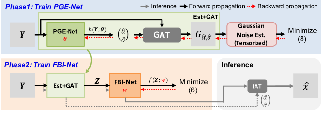
Figure 1: Overall process of FBI-Denoiser.

(2) Training Given the normalized, transformed noisy image $\bm{Z}$, BP-AIDE trains a pixelwise affine denoiser $\bm{f}(\bm{Z};\mathbf{w})\in\mathbb{R}^{n}$, proposed in [12], of which $i$-th reconstruction is

$$f_{i}(\bm{Z};\mathbf{w})=a_{1}(\mathbf{w},\mathbf{C}_{k\times k}^{-i})\cdot Z_{i}+a_{0}(\mathbf{w},\mathbf{C}_{k\times k}^{-i}).$$ (5)

In (5), $\mathbf{C}_{k\times k}^{-i}$ denotes the $k\times k$ noisy patch surrounding ${Z}_{i}$ that excludes $Z_{i}$, and $\{a_{m}(\mathbf{w},\mathbf{C}_{k\times k}^{-i})\}_{m=0,1}$ are the outputs of a specially designed fully convolutional network with parameter $\mathbf{w}$ that takes $\bm{Z}$ as input, but guarantees the exclusion of $Z_{i}$ in the output for location $i$ (i.e., the so-called blind-spot network (BSN)).

Given $m$ distinct (normalized, transformed) noisy images $\mathcal{Z}=\{\bm{Z}^{(j)}\}_{j=1}^{m}$, the training of BP-AIDE is done by minimizing

$$\mathcal{L}(\mathcal{Z};\mathbf{w})=\frac{1}{m}\sum_{j=1}^{m}\mathbf{L}_{n}\Big{(}\bm{Z}^{(j)},\bm{f}(\bm{Z}^{(j)};\mathbf{w});(\beta^{(j)})^{-2}\Big{)},$$ (6)

in which the $\mathbf{L}_{n}(\cdot;\cdot)$ in (6) is defined in [11] as

$$\mathbf{L}_{n}(\bm{Z},\bm{f};{\sigma}^{2})\triangleq\frac{1}{n}{\|\bm{Z}-\bm{f}\|_{2}^{2}}+\frac{{\sigma}^{2}}{n}\sum_{i=1}^{n}(2{a}_{1,i}-1),$$ (7)

in which $\bm{f}\triangleq\bm{f}(\bm{Z};\mathbf{w})$ and $a_{1,i}\triangleq a_{1}(\mathbf{w},\mathbf{C}_{k\times k}^{-i})$ for notational brevity. Now, it is shown in [12, Lemma 1] that if the noise that generates $\bm{Z}$ is additive, independent, zero-mean with homogeneous variance, e.g., AWGN, then (7) becomes an unbiased estimate of the mean-squared error (MSE) of $\bm{f}(\bm{Z};\mathbf{w})$ for estimating the underlying clean image. An important point to emphasize is that such unbiasedness only holds for the pixelwise affine denoisers of the form (5) with $\{a_{m}(\mathbf{w},\mathbf{C}_{k\times k}^{-i})\}_{m=0,1}$ being conditionally independent of $Z_{i}$ given $\bm{Z}^{-i}$ (i.e., the outputs of a BSN). Since the GAT transformed and normalized image $\bm{Z}^{(j)}$ approximately has AWGN with variance $(\beta^{(j)})^{-2}$, minimizing (6), which only depends on the noisy images $\mathcal{Z}$ and no underlying cleans, indeed becomes minimizing the unbiased estimate of MSE. In [10], BP-AIDE simply adopted the BSN architecture proposed in [12] and trained the network for obtaining the pixelwise slope and intercept $\{a_{m}(\mathbf{w},\mathbf{C}_{k\times k}^{-i})\}_{m=0,1}$ for all $i$.

(3) Inference Once the training is done, when denoising a given test noisy image $\bm{Y}_{\text{te}}$ at the inference time, the Est+GAT step is first applied to obtain $\bm{Z}_{\text{te}}$, then gets denoised by $\bm{f}(\bm{Z}_{\text{te}},\mathbf{w}_{\text{BP-ADIE}})$ in the transformed domain. Then, we apply the reverse of the normalization step in Est+GAT to obtain $\bm{D}$ and finally apply the IAT (4) with the estimated noise parameters $(\hat{\alpha},\hat{\sigma})$ obtained in the Est+GAT step.

3.4 Motivation

While BP-AIDE achieved the state-of-the-art denoising performance for real-world noise benchmarks among the methods that only use single noisy images, we observe its critical bottleneck in inference time lies in the Est+GAT step described above. Namely, the Poisson-Gaussian noise parameters $(\alpha,\sigma)$ need to be estimated for each and every given test image, which typically takes in the order of a few seconds using modern CPUs. Moreover, the BSN from [12], denoted by QED network, uses three different kind of masked convolution filters, which results in large memory usage and unnecessary FLOPs that slows down the inference time. As described in the next section, we dramatically improve the inference time of BP-AIDE ($\times 10$) by learning to estimate the Poisson-Gaussian noise parameters with a separate network (PGE-Net) and devising a novel BSN (FBI-Net) with much simpler structure.

4 Main Method

As illustrated in Figure 1, our proposed FBI-Denoiser consists of two phases: first train PGE-Net for Poisson-Gaussian noise estimation (Phase 1), then train FBI-Net for blind denoising (Phase 2). In the subsequent sections, we first present the intuition of and the training procedure of PGE-Net (Section 4.1), then present in details about the new BSN architecture (Section 4.2).

4.1 Training PGE-Net: Phase 1

As mentioned in Section 3.2, GAT [5] is known to stabilize the noise such that the noise for each pixel in the transformed image, $\bm{G}_{\alpha,\sigma}(\bm{Y})$, becomes approximately independent Gaussian with unit variance. We use this property of GAT to build an intuition for training a network to estimate the Poisson-Gaussian noise parameters, $(\alpha,\sigma)$.

Before describing our method, we introduce a few more notations. First, let $\bm{Y}$ denote a noisy image as before that is corrupted by the Poisson-Gaussian noise model (1) with true parameters $(\alpha,\sigma)$. Moreover, define $B$ as a patch extracted from $\bm{Y}$ and $p_{B}(\bm{x})$ as the PDF of the clean $\bm{x}$ over $B$. Moreover, denote $G_{\hat{\alpha},\hat{\sigma}}(\bm{Y})$ as the GAT-transformed image with estimated $(\hat{\alpha},\hat{\sigma})$, and the stabilized noise variance of $\bm{G}_{\hat{\alpha},\hat{\sigma}}(\bm{Y})$ is denoted by $\text{Var}\,(G_{\hat{\alpha},\hat{\sigma}}(\bm{Y})|\bm{x})$. Now, in [31, Proposition 1], it has been shown that, under reasonable assumptions, the following set

$$\mathcal{S}_{B}\triangleq\Big{\{}(\hat{\alpha},\hat{\sigma}):\int\,\sqrt{\text{Var}\,(G_{\hat{\alpha},\hat{\sigma}}(\bm{Y})\,|\,\bm{x})}p_{B}(\bm{x})dx=1\Big{\}}$$

becomes a locally smooth curve around the true noise parameters $(\alpha,\sigma)$. With this proposition, [31] showed that when multiple patches, $\{B_{i}\}$’s, are extracted from an image, then the true $(\alpha,\sigma)$ typically lie in the intersection $\cap_{i}\mathcal{S}_{B_{i}}$.

While the findings of [31] can be applied to estimating true $(\alpha,\sigma)$ for a single image, we extend this intuition for devising a neural network-based estimation method that can learn the estimation function from multiple noisy images. In Figure 2, we show that when the patches $\{B_{i}\}$’s are extracted from multiple noisy images that are corrupted with Poisson-Gaussian noise with the same parameters $(\alpha,\sigma)$, the true $(\alpha,\sigma)$ also tends to lie near the intersection $\cap_{i}S_{B_{i}}$. This observation suggests that we can use patches from multiple noisy images and may learn a neural network model that can directly estimates the noise parameters $(\hat{\alpha},\hat{\sigma})$ that make the noise variance of $G_{\hat{\alpha},\hat{\sigma}}(\bm{Y})$ close to $1$. Furthermore, when sufficiently many noisy images with various levels of $(\alpha,\sigma)$ are available as a training set, we may also expect the neural network to generalize well to unseen noise parameters.

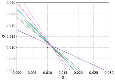
Figure 2: $\mathcal{S}_{B}$ curves for ten patches each cropped from different images randomly selected from the MIT-Adobe FiveK Dataset   [9] (True $(\alpha,\sigma)=(0.01,0.01)$ denoted by x.)

Our PGE-Net exactly realizes the intuition made above. We first define a neural network, $h(\cdot,\bm{\theta}):\bm{Y}\rightarrow\mathbb{R}^{2}$, that takes the Poisson-Gaussian noise corrupted image $\bm{Y}$ and outputs the noise parameter estimates $(\hat{\alpha},\hat{\sigma})$. Moreover, we denote $\eta(\cdot):\bm{Z}\rightarrow\mathbb{R}$ as the function in [15] that estimates the Gaussian noise variance from an input image $\bm{Z}$. Then, given $m$ distinct noisy images $\mathcal{Y}=\{\bm{Y}^{(j)}\}_{j=1}^{m}$, the loss function for our PGE-Net becomes

$$\mathcal{L}_{\text{PGE}}(\mathcal{Y};\bm{\theta})\triangleq\sum_{j=1}^{m}\Big{(}\mathit{\eta}\big{(}G_{\hat{\alpha}(\bm{\theta}),\hat{\sigma}(\bm{\theta})}(\bm{Y}^{(j)})\big{)}-1\Big{)}^{2},$$ (8)

in which $\hat{\alpha}(\bm{\theta})\triangleq h_{1}(\bm{Y}^{(j)};\bm{\theta})$ and $\hat{\sigma}(\bm{\theta})\triangleq h_{2}(\bm{Y}^{(j)};\bm{\theta})$ are the estimated noise parameters $(\hat{\alpha},\hat{\sigma})$ that are outputs of $h(\cdot,\bm{\theta})$. For the specific architecture of $h(\cdot,\bm{\theta})$, we used a three layer U-Net [39] architecture and average pooling layer in the output layer.

Now, when using (8) as a loss function to minimize for training $h(\cdot,\bm{\theta})$, an important point to check is whether all the operations for computing the loss is differentiable with respect to the network parameter $\bm{\theta}$ and can be implemented with tensor operations. To that end, we can see that the GAT (3) can be tensorized by a linear operation and applying an element-wise function. However, implementing the Gaussian noise variance estimation $\eta(\cdot)$ [15] with tensor operations is not trivial since it involves iterative for-loop procedures. To that end, we utilized several tricks using the lower triangular matrix multiplication and masking scheme to replace iterative procedures with tensor operations. Details about the implementations can be found in the Supplementary Material (S.M).

Note the main purpose of PGE-Net is not to simply estimate the noise parameters in a myopic way, but to estimate them fast such that the GAT-transformed image (with the estimated parameters) has stabilized noise variance close to 1 for the next denoisng step. Once our PGE-Net is learned via minimizing (8), it enjoys extremely fast inference time (using GPU) as only simple forward pass of the neural network is required to estimate the noise parameters $(\hat{\alpha},\hat{\sigma})$. Moreover, as we show in Section 5.2, our method becomes much more stable than the conventional noise estimation methods since PGE-Net can smoothly generalize from multiple noisy images, whereas the methods in [20, 28], which run optimization routines separately for each image, may fail to correctly estimate depending on the input image.

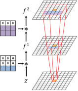
(a) HQ-SSL [24]

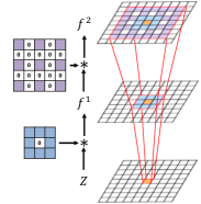
(b) D-BSN [45]

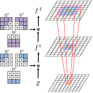
(c) FC-AIDE [12]

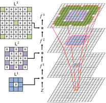
(d) FBI-Net

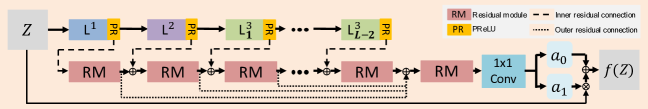
(e) Overall architecture of FBI-Net

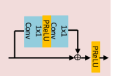
(f) Residual Module

Figure 3: The layers of previously proposed blind spot network and our FBI-Net.

4.2 Training FBI-Net: Phase 2

Once the noise parameters $(\hat{\alpha},\hat{\sigma})$ are estimated with PGE-Net, our denoising network FBI-Net is trained following the same training procedure of BP-AIDE described in Section 3.3 (as also shown in Phase 2 of Figure 1); namely, minimize (6) with the transformed (with the estimated $(\hat{\alpha},\hat{\sigma})$) and normalized images $\bm{Z}^{(j)}$. Recall that the BSN architecture was necessary for implementing the pixelwise affine denoiser (5) and maintaining the unbiasedness of (7), and we devise a more efficient BSN in this section.

The ideal condition for BSN is to have a simple structure that excludes only $Z_{i}$ when computing the activation value at location $i$ in any layer. In practice, some methods implemented BSN by discarding some more pixels other than $Z_{i}$ when computing the activation value at location $i$, but obviously, the more we exclude, the worse the performance becomes. Recently, several network architecture to enhance the efficiency of BSN were proposed [12, 23, 24, 45] in the denoising context. N2V [23] maintains above constraint indirectly by adopting randomly masking scheme. The masking scheme severely degrades training efficiency since only few pixels can be utilized. HQ-SSL [24] suggests a more efficient constrained model by adopting four-way rotations as shown in Figure 3(a). But the requirement of four rotated input images gives limited efficiency. D-BSN [45] devised a completely re-designed model. As shown in Figure 3(b), they mainly use two different types of a masked CNN layer and $1\times 1$ convolution layer to maintain the constraint. This model significantly improves efficiency over previous methods, however, it still has the disadvantage of having a lot of unwanted holes excluded from the receptive field. As shown in Figure 3(c), FC-AIDE [12] designed three different layers, denoted as Q, E and D layer. By utilizing three layers, they obtain the ideal condition we described above. However, since each of the three layers has to be stacked separately for getting it, the model is relatively complex and its inference time is slow.

We propose a more efficient BSN architecture (FBI-Net) by re-designing three different zero-masked convolution layers, L¹, L² and L³ as described in Figure 3(d). L¹ is a center masked $3\times 3$ size of convolution layer which is equal with the first layer proposed in D-BSN. L² is $5\times 5$ size of convolution layer which is all masked except for eight holes and L³ is $7\times 7$ size of convolution layer which only has weights at the center and each edge. Note that L³ can be replaced with $3\times 3$ size of a dilated convolution layer (dilation = 3). By stacking these layer sequentially, we can get an almost full receptive field with fewer holes than D-BSN. Compared with FC-AIDE, even though FBI-Net have some holes in the receptive field, our layers have the advantage of obtaining a simpler architecture and fewer parameters.

Table 2: The comparison of BSN on an image of size 512$\times$512.

	FC-AIDE	D-BSN	FBI-Net
Num of parameters	754,000	6,612,000	340,000
GPU memory requirement	2,581MB	4,231MB	2,512MB
Inference time	0.29	0.99	0.21

Figure 3 shows the overall architecture of FBI-Net. We sequentially stacked layers in the order of L¹, L² and L³ but we only stacked L³ after $4$-th layer. Following the finding of FC-AIDE [12], we used PReLU [22] for all activation functions and Residual Module (RM) proposed in Figure 3(f). To maintain the constraint, we only used $1\times 1$ CNN layer for the output layer and RM. For all experiments, we set $L=17$ which has a receptive field of 181$\times$181 size. Note that we add two different residual connections denoted by Inner and Outer residual connection. We found out that these residual connections make more stable training and improve the denoising performance as can be shown in the ablation study. Table 2 shows the performance comparison of each BSN when denoising an image of size $512\times 512$. Compared to the baselines, the proposed FBI-Net uses much smaller number of parameters and achieves the fastest inference time while the GPU memory requirement is small.

5 Experimental Results

5.1 Data and Experimental settings

Data and Implementation details   In synthetic noise experiments, we used two datasets: BSD400 [32] for grayscale images and MIT-Adobe FiveK Dataset (Fivek) [9] for raw-RGB images. For evaluation of the grayscale images, the standard BSD68 dataset [40] was used. For Fivek, which is composed of $5,000$ images, $4,800$ images were used for training, and the remaining $200$ were used as a test set. To reflect the real noise characteristics, various levels of Poisson-Gaussian noise were simulated. Note each model is individually trained and tested with designated noise characteristics. For real noise experiments, we used three real-world noisy image datasets: Fluorescence Microscopy Denoising (FMD) dataset [49], which is composed of grayscale microscopy images, and SIDD [3] / DND [35] which consist of raw-RGB and sRGB images. In FMD, raw noisy images from three separate general configurations are used; confocal FISH (CF FISH), confocal MICE (CF MICE) and two-photon MICE (TP MICE). The training on SIDD and DND was done using only raw-RGB images, and we received the evaluation results on both raw-RGB and sRGB test sets by submitting the results to the public websites [2, 1], respectively. Note that SIDD provides training, validation and test datasets, but DND only provides test images to the public. For training a model, we generated $m=25,000$ noisy patches of size $210\times 210$ from each dataset. To reflect the complexity of real noise, we reduced the range of slope coefficient $a_{1}(\cdot)$ in (5), i.e., we changed from $[0,1]$ which is the original range of $a_{1}(\cdot)$ suggested by [10] to $[0,0.1]$. For a fair comparison, we used the same range $[0,0.1]$ for both BP-AIDE and FBI-Denoiser in all experiments. The details on the software platform, training and hyperparameters are in the S.M.

Baselines   We first compared the accuracy of the noise parameters from PGE-Net (phase 1) with two representative baselines: Foi [20] and Liu [28]. Then, we compared the overall denoising performance of FBI-Denoiser with following baselines: GAT+BM3D [17], N2V [23], D-BSN [45], and BP-AIDE [10]. GAT+BM3D is a traditional method, but it is still a very powerful baseline for the Poisson-Gaussian noise denoising. The estimation method in Liu [28] is used as a noise estimation method for GAT+BM3D and BP-AIDE, since it achieves robust performance in real-world noise benchmarks. Moreover, the self-supervised step of D-BSN is used as a baseline for fair comparison. As an upper bound, we trained a model in a supervised way (i.e., using clean target images), denoted as "Sup", that uses the same network architecture as FBI-Net. All results of the baselines are reproduced with publicly available source codes, and for brevity, FBI-Denoiser is denoted as “FBI-D” in this section.

5.2 Experimental results on noise estimation

Here, we first validate the effectiveness of the noise estimation of PGE-Net. Table 3 shows the average of the estimated $(\hat{\alpha},\hat{\sigma})$ values, obtained by Foi [20], Liu [28] and PGE-Net from BSD68 images that are corrupted by four different noise levels specified by each row in the table.

Table 3: The average values of estimated $\hat{\alpha}$ and $\hat{\sigma}$ for BSD68. Bold denotes the best result among the three methods.

Noise level $(\alpha,\sigma)$	Foi [20]		Liu [28]		PGE-Net
	$\hat{\alpha}$	$\hat{\sigma}$	$\hat{\alpha}$	$\hat{\sigma}$	$\hat{\alpha}$	$\hat{\sigma}$
(0.1, 0.02)	$0.096$	0.042	$0.072$	$0.045$	0.098	$0.003$
(0.1, 0.0002)	0.097	$0.035$	$0.071$	$0.044$	$0.095$	0.0001
(0.05, 0.02)	0.049	0.031	$0.04$	$0.04$	$0.052$	$0.0001$
(0.05, 0.0002)	0.051	$0.018$	$0.039$	$0.034$	$0.051$	0.0001

In addition, we indirectly measured the performance of noise estimation by comparing the denoising performance (on BSD68 and Fivek) of GAT+BM3D that uses the estimated noise parameters from each estimation method, as shown in Table 4. Moreover, the performance of GAT+BM3D using the ground truth noise level is reported in the table as an upper bound. Firstly, from Table 3, we observed that unlike for $\alpha$, PGE-Net seems to significantly underestimate $\sigma$. However, we observe from Table 4 that GAT+BM3D with the estimated parameters of PGE-Net still shows competitive denoising performance compared to others [20, 28] with much faster inference time ($\times 2000$). This suggests that the underestimated $\hat{\sigma}$ of PGE-Net has little impact on the denoising performance of GAT+BM3D or BP-AIDE framework (which carry out GAT using $\hat{\sigma}$).

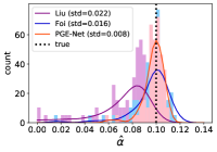
(a) $(\alpha=0.1\,,\sigma=0.02)$

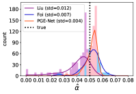
(b) $(\alpha=0.05\,,\sigma=0.0002)$

Figure 4: Histogram of estimated $\hat{\alpha}$ for BSD68 from each estimation method.

As we emphasized in Section 4.1, we believe this somewhat counter-intuitive result is possible since the underestimation of PGE-Net for $\sigma$ turns out to be inconsequential for ensuring that the GAT-transformed image (with the estimated parameters of PGE-Net) has stabilized noise with homogeneous variance close to 1. To verify this more in detail, we conducted an experiment using an additional toy example in S.M.

Table 4: Denoising results of GAT+BM3D with the estimated noise parameters. Red and blue denote the highest and the second highest result among the noise estimation algorithms, respectively.

Dataset (PSNR / SSIM)			Performance of GAT+BM3D
			Foi	Liu	PGE-Net	Ground truth
BSD68	$(\alpha,\sigma)$	(0.01,0.0002)	29.88 / 0.8432	30.33 / 0.8623	30.14 / 0.8521	30.34 / 0.8641
		(0.01,0.02)	29.73 / 0.8393	30.08 / 0.8564	29.81 / 0.8433	30.16 / 0.8570
		(0.05,0.0002)	26.07 / 0.7292	26.16 / 0.7371	26.14 / 0.7335	26.18 / 0.7362
		(0.05,0.02)	26.03 / 0.7269	26.12 / 0.7352	26.11 / 0.7344	26.16 / 0.7349
	Time for noise estimation		3.123s	1.084s	0.002s	-
Fivek	$(\alpha,\sigma)$	(0.0005,0.0002)	43.63 / 0.8645	49.05 / 0.9722	49.11 / 0.9736	49.41 / 0.9764
		(0.0005,0.02)	41.90 / 0.8586	44.51 / 0.9188	44.11 / 0.9144	44.57 / 0.9173
		(0.01,0.0002)	40.24 / 0.8493	42.33 / 0.9170	42.01 / 0.9060	42.46 / 0.9152
		(0.01,0.02)	40.95 / 0.8347	41.26 / 0.8857	41.28 / 0.8863	41.14 / 0.8812
	Time for noise estimation		2.521s	1.812s	0.002s	-

Furthermore, Figure 4 shows the histograms of the $\hat{\alpha}$ values (on BSD68) for two different noise levels obtained by each estimation method. From the figure, we observe that the standard deviations of $\hat{\alpha}$’s obtained by PGE-Net are far smaller than those of others, and, in particular, the failure case (in which $\hat{\alpha}$ goes to zero) does not occur in PGE-Net. Note such failure case of $\hat{\alpha}$ is fatal for training BP-AIDE or FBI-Denoiser since the extremely small value of $\hat{\alpha}$, which is a denominator of GAT (3), causes the gradient explosion.

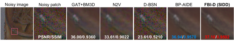
Figure 5: Visualization results of DND

5.3 Experimental results on denoising

Synthetic noise   The experimental results on synthetic raw-RGB Fivek dataset are shown in the top of Table 5. We simulated not only the specified levels of ($\alpha$, $\sigma$), but also a mixture of noise levels denoted as “Mixture noise”, which were generated by following the same procedure as [7] for sampling multiple noise levels. From the results, we first note that our FBI-D performs very well (often the best) compared to other baselines across various noise levels, including the “Mixture noise” case, with a fast inference time. From this result, we can confirm again that PGE-Net is very effective for FBI-D to achieve a competitive denoising performance. Secondly, BP-AIDE and GAT+BM3D also aschieve good results, however, these methods have very slow inference times due to the computational cost of the noise estimation method in Liu [28]. Finally, D-BSN achieves a good performance for the weak noise cases, which surpasses FBI-D, however, when the noise is mixed or strong, D-BSN is far inferior to others. In S.M, we analyze why FBI-D achieves relatively low performance in the weak noise cases.

Table 5: PSNR(dB)/SSIM on Fivek (Synthetic) / FMD (Real) validation dataset. The colored texts are as before.

Dataset			GAT+BM3D	N2V	D-BSN	BP-AIDE	FBI-D	FBI-D (Sup)
Synthetic	Fivek ($\alpha$, $\sigma$)	(0.01, 0.0002)	42.33 /0.9170	30.39 /0.8541	44.50 /0.9602	43.54 /0.9464	44.43 /0.9569	44.80 /0.9600
		(0.01, 0.02)	41.26 /0.8857	29.21 /0.8168	38.06 /0.8280	42.59 /0.9350	43.14 /0.9402	44.38 /0.9537
		(0.05, 0.02)	36.42 /0.8034	25.84 /0.7386	26.13 /0.4363	38.37 /0.9107	39.30 /0.9165	42.17 /0.9402
		Mixture noise	46.94 /0.9560	33.43 /0.8949	39.91 /0.8336	46.43 /0.9658	46.87 /0.9695	47.55 /0.9702
Real	FMD	CF FISH	31.31 /0.8920	31.92 /0.8831	22.86 /0.4479	32.17 /0.8841	32.22 /0.8853	32.98 /0.9111
		CF MICE	37.20 /0.9617	37.54 /0.9611	30.61 /0.7305	38.31 /0.9634	38.32 /0.9637	38.95 /0.9669
		TP MICE	33.76 /0.9157	33.34 /0.9080	26.24 /0.4239	33.89 /0.9023	33.95 /0.9084	34.40 /0.9217
Inference time			5.13s	0.06s	0.99s	2.00s	0.21s

Real-world noise   The results on FMD dataset are reported in the bottom of Table 5. From the table, we observe again that FBI-D consistently outperforms other baselines. Moreover, D-BSN suffers from serious performance degradation, and this illustrates another example of poor applicability of D-BSN when the noise is strong.

Table 6 shows the results on SIDD [3] and DND [35] datasets. In DND, since the $50$ noisy test images are available, we regard this set as both training and test set. Note this is perfectly possible since all methods in Table 6 do not require any clean images for training. In addition, particularly for the DND results, we also report the results of BP-AIDE and FBI-D, which are trained on the training set of SIDD. For clarity, we present two versions of BP-AIDE and FBI-D trained on different datasets; “(SIDD)” and “(DND)” stand for the dataset used for training, respectively. From the table, firstly, we reconfirm the similar tendency as Table 5; i.e., FBI-D mostly dominates other baselines and enjoys fast inference time. Note SIDD and DND datasets contain a mixture of various noise levels, hence, this result shows the robustness and effectiveness of our FBI-D for the real “mismatched” noise case. Secondly, from the strong performance of “FBI-D (SIDD)” for both SIDD and DND, we verify the strong generalization capability of FBI-D. We also note that, as we show in the S.M., the performance of “FBI-D (SIDD)” is also competitive with supervised trained models. Finally, the visualization results in Figure 5 re-emphasize the strength of “FBI-D (SIDD)”; it reconstructs the detailed texture much better than any other baselines.

Table 6: PSNR(dB)/SSIM on SIDD and DND dataset. The colored texts are as before.

Dataset			GAT+BM3D	N2V	D-BSN	BP-AIDE (SIDD)	BP-AIDE (DND)	FBI-D (SIDD)	FBI-D (DND)
Real	SIDD	RAW	48.52 /0.9800	46.30 /0.9760	37.16 /0.8390	50.45 /0.9900	-	50.57 /0.9900	-
		sRGB	34.61 /0.8789	32.85 /0.8470	24.07 /0.4999	37.91 /0.9420	-	38.07 /0.9420	-
	DND	RAW	47.53 /0.9761	45.41 /0.9688	39.63 /0.8642	47.75 /0.9770	47.60 /0.9732	48.02 /0.9787	47.53 /0.9706
		sRGB	37.98 /0.9203	35.82 /0.9022	30.23 /0.7095	38.79 /0.9446	38.60 /0.9259	38.98 /0.9451	38.56 /0.9185
Inference time			5.13s	0.06s	0.99s	2.00s		0.21s

5.4 Ablation study

Ablation study on PGE-Net   Here, we analyze the effect of the loss function of PGE-Net (8) by comparing with the naive supervised estimation model. Table 7 shows the PSNR/SSIM values of GAT+BM3D using estimated noise parameters from different methods on Fivek dataset corrupted with a mixture of noise levels ($\alpha\in[0,0.16^{2}],\sigma\in[0,0.06]$). For comparison, we trained “Sup (MSE)” with exact same architecture as PGE-Net by minimizing the MSE between $(\alpha,\sigma)$ and $(\hat{\alpha},\hat{\sigma})$. The result of PGE-Net overwhelming that of “Sup (MSE)” may seem counter-intuitive, but we verify that when GAT is done with the estimated noise parameters of PGE-Net and “Sup (MSE)”, the average variances of the noise in the transformed images become $1.03$ and $1.58$, respectively. Thus, it turns out that “Sup (MSE)” merely focuses on estimating $\alpha$ and $\sigma$ via minimizing the squared error, but its estimated parameters do not necessarily result in stabilized variance after carrying out GAT using them. We believe this result again shows the effectiveness and strength of our loss function (8) for PGE-Net.

Table 7: Ablation studies of PGE-Net on Fivek (with a mixed noise)

PSNR/SSIM	Foi [20]	Liu [28]	PGE-Net	Sup (MSE)
GAT+BM3D	37.23 / 0.9113	38.58 / 0.9336	38.72 / 0.9350	35.84 / 0.8674

Ablation study on FBI-Net   We demonstrate the necessity of each component of FBI-Net. Table 8 compares the PSNR/SSIM values of the networks with and without each component on Fivek ($\alpha=0.01,\sigma=0.02$). RC and RM denotes Residual Connection and Residual Module, respectively. All networks are trained by a supervised way. From the table, we observe a serious performance degradation when any component of FBI-Net is absent, hence, conclude that RC and RM in our FBI-Net are essential for the successful training of FBI-D.

Table 8: Ablation studies of FBI-Net on Fivek ($\alpha=0.01,\sigma=0.02$).

Component	FBI-Net	Case1	Case2	Case3	Case4	Case5	Case6	Case7
Outer RC	✓	✗	✓	✓	✗	✗	✓	✗
Inner RC	✓	✓	✗	✓	✗	✓	✗	✗
RM	✓	✓	✓	✗	✓	✗	✗	✗
PSNR /SSIM	44.38 /0.9537	44.11 /0.9506	44.31 /0.9529	44.19 /0.9520	44.24 /0.9525	28.82 /0.5103	28.84 /0.5118	28.82 /0.5103

6 Concluding Remarks

We proposed FBI-Denoiser which resolves the computational complexity issue of BP-AIDE by devising PGE-Net, which is much faster than conventional Poisson-Gaussian noise estimation ($\times 2000$), and FBI-Net, which is an efficient blind spot network. We showed FBI-Denoiser achieves the state-of-the-art blind image denoising performance solely based on “single” noisy images with much faster inference time on various synthetic/real noise benchmark datasets.

See pages 1 of fbi_denoiser_supp.pdf See pages 2 of fbi_denoiser_supp.pdf See pages 3 of fbi_denoiser_supp.pdf See pages 4 of fbi_denoiser_supp.pdf See pages 5 of fbi_denoiser_supp.pdf See pages 6 of fbi_denoiser_supp.pdf See pages 7 of fbi_denoiser_supp.pdf See pages 8 of fbi_denoiser_supp.pdf

References

- [1] Dnd Benchmark Website. https://noise.visinf.tu-darmstadt.de/.
- [2] Sidd Benchmark Website. https://www.eecs.yorku.ca/~kamel/sidd/.
- [3] Abdelrahman Abdelhamed, Stephen Lin, and Michael S. Brown. A high-quality denoising dataset for smartphone cameras. In IEEE Conference on Computer Vision and Pattern Recognition (CVPR), pages 1692–1700, 2018.
- [4] Sergey Abramov, Victoriya Zabrodina, Vladimir Lukin, Benoit Vozel, Kacem Chehdi, and Jaakko Astola. Improved method for blind estimation of the variance of mixed noise using weighted lms line fitting algorithm. In IEEE International Symposium on Circuits and Systems (ISCAS), pages 2642–2645, 2010.
- [5] Francis J Anscombe. The transformation of poisson, binomial and negative-binomial data. Biometrika, 35(3/4):246–254, 1948.
- [6] Joshua Batson and Loic Royer. Noise2self: Blind denoising by self-supervision. In International Conference on Machine Learning (ICML), pages 524–533, 2019.
- [7] Tim Brooks, Ben Mildenhall, Tianfan Xue, Jiawen Chen, Dillon Sharlet, and Jonathan T Barron. Unprocessing images for learned raw denoising. In IEEE Conference on Computer Vision and Pattern Recognition (CVPR), pages 11028–11037, 2019.
- [8] Antoni Buades, Bartomeu Coll, and Jean-Michel Morel. A review of image denoising algorithms, with a new one. Multiscale Modeling & Simulation, 4(2):490–530, 2005.
- [9] Vladimir Bychkovsky, Sylvain Paris, Eric Chan, and Frédo Durand. Learning photographic global tonal adjustment with a database of input/output image pairs. In IEEE Conference on Computer Vision and Pattern Recognition (CVPR), pages 97–104, 2011.
- [10] Jaeseok Byun and Taesup Moon. Learning blind pixelwise affine image denoiser with single noisy images. IEEE Signal Processing Letters, 27:1105–1109, 2020.
- [11] Sungmin Cha and Taesup Moon. Neural adaptive image denoiser. In IEEE International Conference on Acoustics, Speech and Signal Processing (ICASSP), pages 2981–2985, 2018.
- [12] Sungmin Cha and Taesup Moon. Fully convolutional pixel adaptive image denoiser. In IEEE International Conference on Computer Vision (ICCV), pages 4160–4169, 2019.
- [13] Sungmin Cha, Taeeon Park, Byeongjoon Kim, Jongduk Baek, and Taesup Moon. Gan2gan: Generative noise learning for blind denoising with single noisy images. In International Conference on Learning Representations (ICLR), 2021.
- [14] Meng Chang, Qi Li, Huajun Feng, and Zhihai Xu. Spatial-adaptive network for single image denoising. In European Conference on Computer Vision (ECCV), pages 171–187, 2020.
- [15] Guangyong Chen, Fengyuan Zhu, and Pheng Ann Heng. An efficient statistical method for image noise level estimation. In IEEE International Conference on Computer Vision (ICCV), pages 477–485, 2015.
- [16] Jingwen Chen, Jiawei Chen, Hongyang Chao, and Ming Yang. Image blind denoising with generative adversarial network based noise modeling. In IEEE Conference on Computer Vision and Pattern Recognition (CVPR), pages 3155–3164, 2018.
- [17] Kostadin Dabov, Alessandro Foi, Vladimir Katkovnik, and Karen Egiazarian. Image denoising by sparse 3-d transform-domain collaborative filtering. IEEE Transactions on Image Processing, 16(8):2080–2095, 2007.
- [18] David L Donoho and Iain M Johnstone. Adapting to unknown smoothness via wavelet shrinkage. Journal of the american statistical association, 90(432):1200–1224, 1995.
- [19] Michael Elad and Michal Aharon. Image denoising via sparse and redundant representations over learned dictionaries. IEEE Transactions on Image Processing, 15(12):3736–3745, 2006.
- [20] Alessandro Foi, Mejdi Trimeche, Vladimir Katkovnik, and Karen Egiazarian. Practical poissonian-gaussian noise modeling and fitting for single-image raw-data. IEEE Transactions on Image Processing, 17(10):1737–1754, 2008.
- [21] Shuhang Gu, Lei Zhang, Wangmeng Zuo, and Xiangchu Feng. Weighted nuclear norm minimization with application to image denoising. In IEEE Conference on Computer Vision and Pattern Recognition (CVPR), pages 2862–2869, 2014.
- [22] Kaiming He, Xiangyu Zhang, Shaoqing Ren, and Jian Sun. Delving deep into rectifiers: Surpassing human-level performance on imagenet classification. In IEEE International Conference on Computer Vision (ICCV), pages 1026–1034, 2015.
- [23] Alexander Krull, Tim-Oliver Buchholz, and Florian Jug. Noise2void-learning denoising from single noisy images. In IEEE Conference on Computer Vision and Pattern Recognition (CVPR), pages 2129–2137, 2019.
- [24] Samuli Laine, Tero Karras, Jaakko Lehtinen, and Timo Aila. High-quality self-supervised deep image denoising. In Advances in Neural Information Processing Systems (NIPS), pages 6968–6978, 2019.
- [25] Jaakko Lehtinen, Jacob Munkberg, Jon Hasselgren, Samuli Laine, Tero Karras, Miika Aittala, and Timo Aila. Noise2noise: Learning image restoration without clean data. In International Conference on Machine Learning (ICML), pages 2965–2974, 2018.
- [26] Pengju Liu, Hongzhi Zhang, Kai Zhang, Liang Lin, and Wangmeng Zuo. Multi-level wavelet-cnn for image restoration. In IEEE Conference on Computer Vision and Pattern Recognition Workshops (CVPRW), pages 773–782, 2018.
- [27] Xinhao Liu, Masayuki Tanaka, and Masatoshi Okutomi. Single-image noise level estimation for blind denoising. IEEE Transactions on Image Processing, 22(12):5226–5237, 2013.
- [28] Xinhao Liu, Masayuki Tanaka, and Masatoshi Okutomi. Practical signal-dependent noise parameter estimation from a single noisy image. IEEE Transactions on Image Processing, 23(10):4361–4371, 2014.
- [29] Julien Mairal, Francis Bach, Jean Ponce, Guillermo Sapiro, and Andrew Zisserman. Non-local sparse models for image restoration. In IEEE International Conference on Computer Vision (ICCV), pages 2272–2279, 2009.
- [30] Markku Makitalo and Alessandro Foi. Optimal inversion of the generalized anscombe transformation for poisson-gaussian noise. IEEE Transactions on Image Processing, 22(1):91–103, 2012.
- [31] Markku Mäkitalo and Alessandro Foi. Noise parameter mismatch in variance stabilization, with an application to poisson–gaussian noise estimation. IEEE Transactions on Image Processing, 23(12):5348–5359, 2014.
- [32] David Martin, Charless Fowlkes, Doron Tal, and Jitendra Malik. A database of human segmented natural images and its application to evaluating segmentation algorithms and measuring ecological statistics. In IEEE International Conference on Computer Vision (ICCV), pages 416–423, 2001.
- [33] Christopher A Metzler, Ali Mousavi, Reinhard Heckel, and Richard G Baraniuk. Unsupervised learning with stein’s unbiased risk estimator. arXiv preprint arXiv:1805.10531, 2018.
- [34] Nick Moran, Dan Schmidt, Yu Zhong, and Patrick Coady. Noisier2noise: Learning to denoise from unpaired noisy data. In IEEE Conference on Computer Vision and Pattern Recognition (CVPR), pages 12064–12072, 2020.
- [35] Tobias Plotz and Stefan Roth. Benchmarking denoising algorithms with real photographs. In IEEE Conference on Computer Vision and Pattern Recognition (CVPR), pages 1586–1595, 2017.
- [36] Tobias Plötz and Stefan Roth. Neural nearest neighbors networks. In Advances in Neural Information Processing Systems (NIPS), pages 1087–1098, 2018.
- [37] Stanislav Pyatykh, Jürgen Hesser, and Lei Zheng. Image noise level estimation by principal component analysis. IEEE Transactions on Image Processing, 22(2):687–699, 2012.
- [38] Yuhui Quan, Mingqin Chen, Tongyao Pang, and Hui Ji. Self2self with dropout: Learning self-supervised denoising from single image. In IEEE Conference on Computer Vision and Pattern Recognition (CVPR), pages 1890–1898, 2020.
- [39] Olaf Ronneberger, Philipp Fischer, and Thomas Brox. U-net: Convolutional networks for biomedical image segmentation. In International Conference on Medical Image Computing and Computer Assisted Intervention (MICCAI), pages 234–241, 2015.
- [40] Stefan Roth and Michael J Black. Fields of experts: A framework for learning image priors. In IEEE Conference on Computer Vision and Pattern Recognition (CVPR), pages 860–867, 2005.
- [41] Shakarim Soltanayev and Se Young Chun. Training deep learning based denoisers without ground truth data. In Advances in Neural Information Processing Systems (NIPS), pages 3257–3267, 2018.
- [42] Ying Tai, Jian Yang, Xiaoming Liu, and Chunyan Xu. Memnet: A persistent memory network for image restoration. In IEEE International Conference on Computer Vision (ICCV), pages 4539–4547, 2017.
- [43] Mikhail L Uss, Benoit Vozel, Vladimir V Lukin, and Kacem Chehdi. Image informative maps for component-wise estimating parameters of signal-dependent noise. Journal of Electronic Imaging, 22(1):013019, 2013.
- [44] Zhou Wang, Alan C Bovik, Hamid R Sheikh, and Eero P Simoncelli. Image quality assessment: from error visibility to structural similarity. IEEE Transactions on Image Processing, 13(4):600–612, 2004.
- [45] Xiaohe Wu, Ming Liu, Yue Cao, Dongwei Ren, and Wangmeng Zuo. Unpaired learning of deep image denoising. In European Conference on Computer Vision (ECCV), pages 352–368, 2020.
- [46] Syed Waqas Zamir, Aditya Arora, Salman Khan, Munawar Hayat, Fahad Shahbaz Khan, Ming-Hsuan Yang, and Ling Shao. Cycleisp: Real image restoration via improved data synthesis. In IEEE Conference on Computer Vision and Pattern Recognition (CVPR), pages 2696–2705, 2020.
- [47] Kai Zhang, Wangmeng Zuo, Yunjin Chen, Deyu Meng, and Lei Zhang. Beyond a gaussian denoiser: Residual learning of deep cnn for image denoising. IEEE Transactions on Image Processing, 26(7):3142–3155, 2017.
- [48] Yulun Zhang, Kunpeng Li, Kai Li, Bineng Zhong, and Yun Fu. Residual non-local attention networks for image restoration. In International Conference on Learning Representations (ICLR), 2019.
- [49] Yide Zhang, Yinhao Zhu, Evan Nichols, Qingfei Wang, Siyuan Zhang, Cody Smith, and Scott Howard. A poisson-gaussian denoising dataset with real fluorescence microscopy images. In IEEE Conference on Computer Vision and Pattern Recognition (CVPR), pages 11710–11718, 2019.
- [50] Magauiya Zhussip, Shakarim Soltanayev, and Se Young Chun. Extending stein’s unbiased risk estimator to train deep denoisers with correlated pairs of noisy images. In Advances in Neural Information Processing Systems (NIPS), pages 1465–1475, 2019.
- [51] Daniel Zoran and Yair Weiss. From learning models of natural image patches to whole image restoration. In IEEE International Conference on Computer Vision (ICCV), pages 479–486, 2011.