Inference for multi-valued heterogeneous treatment effects when the number of treated units is small

Abstract

We propose a method for conducting asymptotically valid inference for treatment effects in a multi-valued treatment framework where the number of units in the treatment arms can be small and do not grow with the sample size. We accomplish this by casting the model as a semi-/non-parametric conditional quantile model and using known finite sample results about the law of the indicator function that defines the conditional quantile. Our framework allows for structural functions that are non-additively separable, with flexible functional forms and heteroskedasticy in the residuals, and it also encompasses commonly used designs like difference in difference. We study the finite sample behavior of our test in a Monte Carlo study and we also apply our results to assessing the effect of weather events on GDP growth.

1 Introduction

Many applications in economics and elsewhere require us to acknowledge and learn about treatment effect heterogeneity. Particularly in panel data where individuals, firms, or states can have different characteristics, belong to different groups or adopt the treatment in different instances. Moreover, in this setup, outcomes may be depend not only on the current treatment status but on the whole past history of treatment , thereby given raise to multi-valued treatments rather than simple binary ones.

These features — the heterogeneity and the multi-valued nature of treatments — force the researcher to dissagregate the data in a way that the treatment groups can have a small number of units even for moderate and even large sample sizes. Moreover, this issue becomes even more salient if one disaggregates further, for instance, by conditioning on observed characteristics of the individuals to handle potential heterogeneity of the treatment affects. Thus, in these cases, standard inferential procedures that rely on asymptotic results may be untrustworthy or even invalid. The main contribution of this paper is to address this problem by proposing a valid inference method for testing the treatment effect over outcomes that is valid when the number of treated units is small even though the sample size is large. We do so in a potential outcomes framework that is sufficiently general to allow for non-/semi-parametric models with multi-valued heterogeneous treatments and dynamic treatment effects, and to to cover commonly used identification approaches such as RCTs, difference in difference and control variable.

We consider a panel data potential outcomes framework (Neyman et al. [1923/1990]) wherein the so-called outcome function relates the current outcome to the treatment profile — i.e., the current and past treatment status — past outcomes and characteristics of the individual (both observed and unobserved). Under our assumptions, this outcome function is the object of interest as it encodes the causal effect of the treatment profile on current outcomes. In fact, the null hypothesis boils down to whether the outcome function for user-specified treated groups — defined by the observed characteristics and treatment profile — coincides with the outcome function associated to a benchmark/control group.

An important first step in our method is to relate this outcome function for a given treatment group to the solution of a conditional moment restriction defined by the conditional quantile of the current outcome, given the past outcomes and other observed covariates for this group. As a consequence, we are able to construct a test statistic that is akin to a model specification test statistic for non-parametric GMM models where we input an estimator of the outcome function for the benchmark/control group on the moments of the treated groups and reject the null if these moments are far away from zero. The non-standard part of the test lies on approximating its distribution; to do this we employ two insights. First, we note that since the number of treatment groups is finite and fixed, for sufficiently large sample sizes the number of observations will be large in at least one of the groups; we normalize such a group to be the benchmark/control group. Based on this observation, we construct a consistent sieve-based estimator (cf. Chen and Pouzo [2012], Chen et al. [2003]) of the outcome function for such group. Under our assumptions this estimator converges to the true outcome function, but since the effective sample size of each treated group does not grow with the number of units in the overall sample, standard approximations results like the Central Limit Theorem do not apply. To circumvent this issue our second insight is to apply the results by Chernozhukov et al. [2009] to show that the conditional quantile for the treated groups evaluated in the outcome function of the control group, under the null, has a known distribution that can be approximated by simulations. Based on these logic we are able to prove the main result of the paper stating that our test has correct asymptotic size, even if the number of units in the treatment groups stays fixed. In addition, we are also able to construct confidence regions for certain semi-parametric models wherein the treatment effect is encoded in a finite dimensional vector.

The key assumption used to link the outcome function, which is a structural object, to the conditional quantile of the respective groups, which is related to the properties of observed random variables, imposes that some quantile of the random variable representing the unobserved characteristics does not depend on the treatment profile once we condition on observed characteristics and past outcomes. Even though this assumption does restrict the scope of our framework, it still allows for commonly used designs such as RCTs and difference in difference and the control function approach (see Section 5 for an application).

We are not the first paper to propose inference methods that are valid for finite samples. Closest to our methodology is the paper by Ferman and Pinto [2019] which belongs to a strand of the literature that proposes inference methods when the treatment group is small but the control group is large (e.g. Donald and Lang [2007], Conley and Taber [2011] and Cameron et al (2008).). Both, us and this literature, leverage the observations in the control group — for which the number of observations is assumed to be large when the sample size is large — to learn certain features of the problem and then, under the null, extrapolate this knowledge to the treated groups. The difference lies on how we accomplish this. This literature focuses on linear models within a difference in difference framework and imposes, to different degrees, restrictions on the conditional CDF of the residuals given observables, in particular in terms of its heterosckedasticity. In contrast, by casting the problem within a non-parametric conditional quantile moments framework, we are able to perform this extrapolation without imposing any functional form restrictions in the outcome function. The outcome function can be non-separatively additive, can depend on both finite and infinite dimensional parameters and allow for flexible — albeit not completely unrestricted — conditional distribution in the residuals. On the other hand, Ferman and Pinto [2019] allow for within group dependence, whereas we assume units to be IID.

In Section 7 we apply our framework to a two way fixed effect (TWFE) model with heterogeneous treatment effects under staggered adoption, which has been recently studied in many papers (e.g. de Chaisemartin and D’Haultfœuille [2020], Sun and Abraham [2020], Callaway and Sant’Anna [2018], Athey and Imbens [2018]). This literature emphasizes identification, estimation and inference of treatment effects allowing for certain types of heterogeneity and dynamics. To the best of our knowledge all of these papers rely on standard asymptotic theory which assumes that the size of the treated groups grows with the sample size. Given the dynamic nature of treatment profiles and the group heterogeneity of effects, having a small number of treated units could be a salient feature in many applications. Hence, the results in this paper could complement this literature by offering a novel and alternative method for inference.

Related Literature

Beyond the aforementioned papers, our paper builds on and contributes to three main strands of the literature about treatment effects. First, our setup is similar to the one consider by Han [2018]. However, Han [2018] focuses on identification in an IV approach whereas we focus on estimation and testing under a control variable approach when the number of treated units is small.

There is a vast literature concerned with inferential methods that have finite sample properties such as Fisher randomization or permutation methods (see Rosenbaum et al. [2010] for a review). These methods, however, are quite different to our approach as they are derived under a different set of assumptions that impose certain symmetry or invariance of the data distribution under the null (see Hahn and Shi [2017] for a discussion in the context of synthetic control models). We refer the reader to Ferman and Pinto [2019] for a more thorough literature review and references.

From a technical point of view, our results can be viewed as deriving the asymptotic distribution of a test statistic constructed upon a GMM criterion function in a non-parametric conditional moment model, where each of the moments in the (sample) GMM criterion function (which in our case are given by the conditional quantiles of the outcome given observable characteristics for each treatment group) may have different and even non-vanishing rates of convergence, even as the sample size goes to infinity. To our knowledge, the asymptotic results in the non-parametric conditional moment models literature (cf. Ai and Chen [2003], Chen et al. [2003], Chen and Pouzo [2012] and Horowitz and Lee [2007] among many others) do not apply. To bridge this gap, we combine this framework with the finite sample results by Chernozhukov et al. [2009].

2 Illustrative Example

We now present a simple canonical model, which encompasses several existing applications, and which we develop and extend throughout the paper to illustrate different concepts.

Example 1 (Canonical Example).

For each unit $i$ and time $t$, let $Y_{i,t}$ be the economic outcome of interest and let $D_{i,t}$ be a binary variable that encodes the treatment status for this unit at time $t$. We postulate that, for some $L,P\in\mathbb{N}\cup\{0\}$,

$$Y_{i,t}=\kappa+\sum_{s=0}^{L}\theta_{s}D_{i,t-s}+\sum_{s=1}^{P}\gamma_{s}Y_{i,t-s}+\epsilon_{i,t}.$$ (1)

in which $(\theta_{s})_{s=0}^{L}$ are the parameters of interest as they summarize effect of the treatment on the outcome variable.

Similar models have been used in several applications. For instance, to capture the effect that weather has on GDP or GDP growth (Dell et al. [2012], Dell et al. [2014] and references therein); or the effect that climate shocks (Miguel et al. [2004], Burke et al. [2015]) or economic shocks (Bazzi and Blattman [2014]) have on conflicts; or the effect that democratization has on GDP growth (Acemoglu et al. [2019]); or the effect that elections on bond issuance have on economic outcomes such as spending in infrastructure or prices of houses (Cellini et al. [2010]).

Our point of departure is to cast this as a multi-treatment effect problem where there are $\{0,1\}^{L+1}$ potential outcomes, each indexed by a particular treatment profile, i.e., $Y_{t}(d_{t},...,d_{t-L})$. While several of the aforementioned applications use $L$ equal to 0, 1 or 2, the treatment variables (e.g. climate variables, democratizations, economic shocks, etc) may be highly autocorrelated thus give raise to an omitted variable bias; this has already been pointed out (e.g. Burke et al. [2015]). One way to address this issue is to consider large values of $L$ or even set $L=t$ and let the data determined which lags matter. In these cases, however, the number of countries in each “treatment profile bin” may be very small. In order to illustrate this feature, we use data from Dell et al. [2012] and first encode temperature increases as a binary variable. We define that country $i$ suffered a temperature increase in period $t$ if the difference in temperature between periods $t-1$ and $t$ is above one degree Celsius. We specify $L=4$ and tally the number of countries in each treatment profile for three different time periods, which we report in Table 1 presents the results. For all the choices of $t$ the number of observations in the control group (i.e, the profile with all zeros) is large, however, for each of the other treatment profiles the number of observations is much smaller — in all cases less than 20 and in many less than 10 — even though the sample size is moderate and $L$ is not particularly big.

Profile	N 1960-1964	N 1980-1984	N 1990-1994
00000	100	113	93
00001	7		17
00010	1	5	3
01000	4	1
01001	1
10000	7	1	6
10100	4
00100		3	1
01010		1
00011			1
00101			2
10001			1

Table 1: Number of countries for each treatment profile with $L=4$ and for different periods $t\in\{1964,1984,1994\}$. Empty cells mean no countries for that profile. Data: Panel of 124 countries taken from Dell et al. [2012].

Without further restrictions on the coefficients $(\theta_{s})_{s=1}^{L}$, this feature will render the usual asymptotic techniques untrustworthy or directly unviable. Of course, by imposing additional restrictions on the coefficients $(\theta_{s})_{s=1}^{L}$ — e.g. $\theta_{s}=\theta$ for all $s$ — one can use the linearity assumption to extrapolate; these further restrictions, however, may not be warranted in many applications. The goal of this paper is to propose an inference method that delivers correct results in these situations where the number treated units may be small, even asymptotically. $\triangle$

3 Setup

Our point of departure is a simplified version of the setup in Han [2018] which is in turn an extension of the setup considered by Chernozhukov and Hansen [2005]. This setup corresponds to a potential outcomes framework with multiple treatments.

We consider a panel structure in which for each unit, indexed by $i\in\mathbb{N}$, we observe $T$ time periods of data; we define $\mathbb{T}:=\{1,...,T\}$ as the set of time periods. For each $t\in\mathbb{T}$, a time $t$ treatment profile is a sequence in $\{0,1\}^{t}$, ${D}^{t}:=(D_{1},...,D_{t})$, such that the $s$-th element, $D_{s}\in\{0,1\}$ indicates the treatment status at time $s$. We use ${D}^{t}_{i}$ to denote the time $t$ treatment profile of unit $i\in\mathbb{N}$.

For each $t\in\mathbb{T}$ and time $t$ treatment profile, $d^{t}$, we use $Y_{t}(d^{t})\in\mathbb{Y}\subseteq\mathbb{R}$ to denote the $d^{t}$ potential outcome, that is the outcome at time $t$ had the time $t$ treatment profile been $d^{t}$. We use $Y_{i,t}(d^{t})$ to denote the $d^{t}$ potential outcome of unit $i\in\mathbb{N}$. Finally, let ${Y}^{t}(d^{t}):=(Y_{1}(d^{1}),...,Y_{t}(d^{t}))$. For each $t\in\mathbb{T}$, the time $t$ (observed) outcome profile is given by ${Y}^{t}:=(Y_{1},...,Y_{t})$ where $Y_{t}:=Y_{t}({D}^{t})$.

Finally, for each $t\in\mathbb{T}$, let ${X}^{t}:=(X_{1},...,X_{t})\in\mathbb{X}^{t}$ with $\mathbb{X}\subseteq\mathbb{R}^{q}$ be the vector of observed covariates up to time $t$. We assume the covariates are discrete, i.e., $|\mathbb{X}|<\infty$. While it is straightforward to extend our framework to handle both continuous and discrete covariates — provided the former are not used to define the treatment groups (see Remark 3 below for more details) —, we maintain the assumption of discrete covariates to simplify some of the derivations and exposition, as well as to ease the notational burden.

We now impose restrictions on the process for the treatment and potential outcomes profiles. For each $t\in\mathbb{T}$, let

$$D_{t}=\delta_{t}({Y}^{t-1},X^{t},D^{t-1},V_{t})$$ (2)

where $V^{t}:=(V_{1},...,V_{t})$ are random variables that amount to the shocks for the treatment profiles. Expression 2 allows for dynamic treatment assignments whereby the treatment status at time $t$ can depend on past outcomes, past treatment status and a random shock.

We assume that the process for $Y_{t}(.)$ satisfies

$$Y_{t}(d^{t})=\mu_{t}(Y^{t-1}(d^{t-1}),X^{t},d^{t},U_{t}(d^{t})),\leavevmode\nobreak\ \forall d^{t}\in\{0,1\}^{t},$$ (3)

where $U_{t}(d^{t})$ is a random variable with support in $[0,1]$ whose CDF will be specified below, and it should be viewed as unobserved characteristics of the individual. We can view the vector $(X^{t},U_{t}(d^{t}))$ as the characteristics of the unit, and thus the outcome function, $\mu_{t}$, determines how these characteristics, the time $t$ treatment profile and the past (potential) outcomes affect the current outcome. In particular, under the assumptions below, the mapping

$$d^{t}\mapsto\mu_{t}(Y^{t-1}(d^{t}),x^{t},d^{t},\tau)$$

measures the causal effect of the treatment profile $d^{t}$ on the outcomes, for a unit with characteristics $(x^{t},\tau)\in\mathbb{X}^{t}\times(0,1)$.

We impose the following assumptions on the DGP.

Assumption 1 (IID).

For each $i\in\mathbb{N}$, $((Y_{i,t}(d^{t}),U_{i,t}(d^{t}))_{t,d^{t}},D^{T}_{i},X^{T}_{i},V^{T}_{i})$ are IID drawn from $P$, such that expressions 2 and 3 hold and $D_{0}$ and $Y_{0}(.)$ are assumed to be exogenous.

Assumption 2 (Monotonicity).

$u\mapsto\mu_{t}(y^{t-1},x^{t},d^{t},u)$ is increasing.

Assumption 3 (Conditional Rank Invariance restriction).

For any $d^{t}\in\{0,1\}^{t}$ and some $\tau\in(0,1)$, the distribution of $U_{t}(d^{t})$ conditional on $Y^{t-1}(d^{t-1}),X^{t}$ and $D^{t}$ satisfies the following restriction,

$$P(U_{t}(d^{t})\leq\tau\mid Y^{t-1},X^{t},D^{t})=\tau.$$

Remark 1 (Discussion of the Assumptions).

These assumptions are standard in the literature of conditional quantile estimation and are use to link the structural function to a conditional quantile restriction on the observables. Assumption 1 is the standard IID assumption and can be somewhat relaxed; Lemmas 7 and 8 in Appendix B.2.2 illustrate what aspects of this assumption are used in the proofs. Assumption 2 imposes a monotonicity restriction on the structural function; cf. Chernozhukov and Hansen [2005].

The key assumption is Assumption 3, which conflates two restrictions on the distribution of $U_{t}(d^{t})$ for each $d^{t}$. First, a shape restriction that requires, the $\tau$-th quantile of the CDF of $U_{t}(d^{t})$ given $Y^{t-1},X^{t}$ and $D^{t}=d^{t}$ to be equal to $\tau$. Second, an invariance restriction that requires the $\tau$-th quantile of the CDF of $U_{t}(d^{t})$ given $Y^{t-1},X^{t}$ to be the same for each treatment profile $D^{t}$ (not just $D^{t}=d^{t}$). While it is only the first restriction that is used to show our results, it is the second restriction that warrants the qualifier causal when describing the function $\mu_{t}$; this last point is discussed further in Remarks 5 and 6 below. In essence, this last restriction can be interpreted as a type of selection on observables, in which the observed characteristics are $Y^{t-1},X^{t}$. While this restriction is by no means innocuous and rules out many models, given the general specification of our model, it still allows for many popular approaches like RCTs and difference in difference designs (see Section 5) and control variable approach in general.

To shed more light onto this assumption, we now discuss it under different laws for the treatment profiles and the assumption — to simplify the presentation — that $(U_{t}(d^{t}))_{t}$ are independent across time. First, consider the case where $D^{t}$ is independent of $(U_{t}(d^{t}))_{t,d^{t}}$, e.g., $D_{t}=\delta_{t}(X^{t},D^{t-1},V_{t})$ with $V_{t}$ being independent of $U_{t}(d^{t})$. In this case, conditioning on $Y^{t-1}(d^{t-1})$ is not needed and can be omitted, and thus Assumption 3 boils down to

$$P(U_{t}(d^{t})\leq\tau\mid X^{t})=\tau.$$

This expression is a shape-restriction in the distribution of $U_{t}(d^{t})$ given $X^{t}$, which essentially amounts to a re-normalization of $\mu_{t}$ under the assumption that this distribution is increasing. Moreover, it is straightforward to check that an analogous conclusion can be reached when $D^{t}$ is independent of $U_{t}(d^{t})$ conditional on $Y^{t-1}$; in this case the shape-restriction is over the distribution of $U_{t}(d^{t})$ given $(Y^{t-1},X^{t})$. While these cases cover many applications, there are many other applications where $V_{t}$ is not independent of $U_{t}(d^{t})$. In this case, $V^{t}$ can be viewed as a control variable, and Assumption 3 is analogous to the control function framework for quantile regression (e.g. Lee [2007]). All three cases are further illustrated in Example 3 below. $\triangle$

We now use example 1 to illustrate the outcome function and verify the assumptions.

Example 2 (Canonical Example: Verification of Assumptions 2 and 3).

We now verify Assumptions 2 and 3 in the setup of Example 1 and by doing so illustrate how the structural function looks for this example. To do this we need to impose some restrictions. First, we assume that, for each $t\in\mathbb{T}$, given $Y_{t-1}$, $\epsilon_{t}$ is independent of $D^{t-1}$, $\epsilon^{t-1}$ and $Y^{t-2}$. This assumption can be somewhat relaxed to allow for a richer dependence on past outcomes, but, due to the non-linear nature of our framework, the standard assumption of $E[\epsilon_{t}\mid D^{t}]=0$ will typically be insufficient to verify assumption 3. Let $F(.|.)$ be the conditional CDF of $\epsilon_{t}$ given $Y_{t-1}$, which we assume is an increasing function of $\epsilon$.

Let $U_{t}:=U_{t}(d^{t}):=F(\epsilon_{t}\mid Y_{t-1})$. It is straightforward to verify the following relationship: For any $u\in(0,1)$,

$$P(U_{t}\leq u\mid Y^{t-1}(d^{t-1}),D^{t}=d^{t})=P(\epsilon_{t}\leq F^{-1}(u\mid Y_{t-1}(d^{t-1}))\mid Y^{t-1}(d^{t-1}),D^{t}=d^{t})=u.$$

Thus, Assumption 3 holds. Let $(y^{t-1},d^{t},u)\mapsto\mu_{t}(y^{t-1},d^{t},u):=\kappa+\sum_{s=0}^{L+1}\theta_{s}d_{t-s}+\sum_{s=1}^{P}\gamma_{s}y_{t-s}+F^{-1}(u\mid y_{t-1})$. It is straightforward to check that this choice satisfies Assumption 2 and that $Y_{t}=\mu_{t}(Y^{t-1},D^{t},U_{t})$ coincides with 1. Note that $\mu_{t}$ is indexed by $(\kappa,(\theta_{s})_{s=1}^{L},(\gamma_{s})_{s=1}^{P})$ and the function $F$.

We observe that this specification allows the residual $\epsilon_{t}$ to be heterosckedastic and correlated with lags of the outcome variable. The cost of such flexibility is the estimation of the function $F^{-1}$. Indeed, if $\epsilon_{t}$ is assumed to be IID, the structural function reduces to $(y^{t-1},d^{t})\mapsto\mu(y^{t-1},d^{t},\tau)=\kappa+\sum_{s=0}^{L}\theta_{s}d_{t-s}+\sum_{s=1}^{P}\gamma_{s}y_{t-s}+F^{-1}(\tau)$, which is entirely parameterized by finite dimensional parameters.

Finally, we note that $F^{-1}(u\mid Y_{t-1})$ is the $u$-th conditional quantile of $\epsilon_{t}$ given $Y_{t-1}$. Thus, the structural function $\mu_{t}(\cdot,\cdot,u)$ coincides with the conditional quantile function in Lee [2007] (see equation 4). This fact is present in many of the examples below and it illustrates the link between our framework and a quantile regression model under the control function approach. $\triangle$

The next example illustrates different examples of the process for $(D_{t})_{t=1}^{T}$.

Example 3 (Canonical example: The process for $(D_{t})_{t=1}^{T}$).

Expression 2 allows for many specifications for the treatment process. One simple case is where $D^{T}$ is exogenous but autocorrelated, e.g., for all $t\in\mathbb{T}$, $D_{t}=\delta_{t}(D^{t-1},V_{t})$ where $V^{T}$ is IID. In some applications, however, this assumption might be too strong, as $D_{t}$ could depend not only on past realizations of itself but also on past outcomes. For these applications we can set $D_{t}=\delta_{t}(Y^{t-1},D^{t-1},V_{t})$ where $V^{T}$ is assumed to be IID. Observe that, conditional on $Y^{t-1}$, $D_{t}$ is independent of $U_{t}(d^{t})$. Finally, our framework allows for more general situations where $V^{t}$ is correlated with the error in the outcome equation.

We illustrate this case in a standard election setup, i.e., $D_{t}=1\{X_{t}\geq 0.5\}$ with $X_{t}$ being the shares of votes, but with the additional feature that past election outcomes can influence the voting behavior, i.e., $X_{t}:=m(D_{t-1},V_{t})$ for some function $m$. The “election shock” $V_{t}$ is independent across time but can be correlated with $\epsilon_{t}$ in the outcome equation. Under the condition that the conditional CDF of $\epsilon$ given $X$, $F(.|.)$, is increasing on $\epsilon$, assumptions 2 and 3 hold in this case with $U_{t}:=F(\epsilon_{t}|X_{t})$ and

$$(y^{t-1},x^{t},d^{t},u)\mapsto\mu_{t}(y^{t-1},x^{t},d^{t},u):=\kappa+\sum_{s=0}^{L}\theta_{s}d_{t-s}+\sum_{s=1}^{P}\gamma_{s}y_{t-s}+F^{-1}(u\mid x_{t}),$$

because, for any $u\in(0,1)$ any $Y^{t-1}$, and any $X^{t}$ such that $1\{X_{s}\geq 0.5\}=D_{t}\leavevmode\nobreak\ \forall s\leq t$,

$$P(U_{t}(d^{t})\leq u\mid Y^{t-1},D^{t},X^{t})=E[1\{U_{t}(d^{t})\leq u\}\mid X_{t}]=E[1\{\epsilon_{t}\leq F^{-1}(u|X_{t})\}\mid X_{t}]=u.$$

$\triangle$

Finally, we provide some extensions of example 1 to illustrate the scope of our framework. The first of these extensions shows that it allows for specifications that go beyond additive-separable models.

Example 4 (Canonical example: Quantile Regression).

In Example 1 we study the conditional mean of the economic outcome given past realizations of the treatment (and other variables). However, it could be of interest to also assess the effect of the treatment on other aspects of the outcome distribution. To do this, we consider the following quantile regression model.

$$Y_{i,t}=\kappa(U_{i,t})+\sum_{s=0}^{L}\theta_{s}(U_{i,t})D_{i,t-s}+\sum_{s=1}^{P}\gamma_{s}(U_{i,t})Y_{i,t-s}+U_{i,t}$$

where $U_{i,t}\sim U(0,1)$. It is easy to show that the $\tau$-quantile of $Y_{t}$ given $(D_{s})_{s=t-L}^{t}$ and $(Y_{s})_{s=t-P}^{t-1}$ is given by $\kappa(\tau)+\sum_{s=0}^{L}\rho_{s}(\tau)D_{t-s}+\sum_{s=1}^{P}\gamma_{s}(\tau)Y_{t-s}$, that Assumption 3 holds and that $(y^{t-1},d^{t})\mapsto\mu_{t}(y^{t-1},d^{t},\tau)=\kappa(\tau)+\sum_{s=0}^{L}\theta_{s}(\tau)d_{t-s}+\sum_{s=1}^{P}\gamma_{s}(\tau)y_{t-s}+\tau$. Moreover, under the assumption that $\kappa(\cdot)$, $\theta_{s}(\cdot)$ and $\gamma_{l}(\cdot)$ are increasing for all $s\in\{0,...,L\}$ and $l\in\{1,...,P\}$, Assumption 2 holds. Observe that as opposed to the linear case studied in Example 2, the structural function, $\mu_{t}(\cdot,\cdot,\tau)$ is only indexed by finite dimensional parameters. $\triangle$

The second of these extensions shows how our framework can handle richer specifications with less functional form restrictions.

Example 5 (Canonical example: More general functional form).

In many applications the correct order of lagged outcomes is unknown, and it is not even clear that the lagged outcomes affect current outcomes linearly. Thus, a possible extension for the specifications in Examples 1 and 4 is given by

$$Y_{t}(d^{t})=\sum_{s=0}^{t}\theta_{s}d_{t-s}+\varphi(Y^{t-1}(d^{t-1}),X^{t},\epsilon_{t}(d^{t}))$$

where $\epsilon\mapsto\varphi(y^{t-1},x^{t},\epsilon)$ is an unknown increasing function, and $\epsilon$ is such that its $\tau$-th conditional quantile given $(Y^{t-1},X^{t},D^{t})$ equals $q(Y^{t-1},X^{t})$. This specification can be handled by our framework by defining $U_{t}(d^{t}):=\varphi(Y^{t-1}(d^{t-1}),X^{t},\epsilon_{t}(d^{t}))-\varphi(Y^{t-1}(d^{t-1}),X^{t},q(Y^{t-1}(d^{t-1}),X^{t}))+\tau$ and $\mu_{t}(y^{t-1},x^{t},d^{t},u):=\sum_{s=0}^{t}\theta_{s}d_{t-s}+\kappa(y^{t-1},x^{t})+u$ where $\kappa(y^{t-1},x^{t}):=\varphi(y^{t-1},x^{t},q(y^{t-1},x^{t}))-\tau$; it is to see that Assumptions 1-3 hold. Under these assumptions $\sum_{s=0}^{t}\theta_{s}d_{t-s}$ is the $\tau$-th quantile treatment effect (cf. Chernozhukov and Hansen [2005]) and would be the object of interest and $\kappa$ would be a nuisance (infinite dimensional) parameter.

Implicit in this specification — as well as those in Examples 1 and 4 — lies the assumption that the treatment effect function, $d^{t}\mapsto\sum_{s=0}^{t}\theta_{s}d_{t-s}$, is the same for each observed characteristic and linear on the treatment profile; e.g., the treatment effect for $d^{t}=(1,1,0,...,0)$ is the same as the sum of the effects for $(1,0,0,...,0)$ and $(0,1,0,...,0)$. In some applications these restrictions may be too strong as they restrict potential sources of heterogeneity of treatment effects. For instance — in the context of the applications mentioned in Example 1 — the effect of having two (or more) consecutive weather/climate shocks may have a larger effect on GDP growth than the sum of the effects of each individual shock. To account for this heterogeneity, we can consider the following “saturated” model,

$$Y_{t}(d^{t})=\sum_{\tilde{d}^{t}\in\{0,1\}^{t}}\theta(\tilde{d}^{t},X^{t})1\{\tilde{d}^{t}=d^{t}\}+\varphi(Y^{t-1}(d^{t-1}),X^{t},\epsilon_{t}(d^{t})),$$

where $\theta(d^{t},x^{t})$ is the $\tau$-th quantile treatment effect for $x^{t}$. In our empirical application in Section 7, we employ a (simplified) version of this saturated model to study the effect on weather shocks on GDP growth. $\triangle$

Henceforth, we will typically omit the $t$ index for the functions $\mu_{t}$ and $\delta_{t}$.

3.1 The object of interest and null hypothesis

In this paper, we want to test the hypothesis whether the effect of an specific set of treatment profiles, $\mathcal{D}^{t}\subseteq\{0,1\}^{t}$, is the same as effect of the control treatment profile, $0^{t}$, for all units that share the same characteristics $(x^{t},\tau)$.

Formally,

$$H_{0}\leavevmode\nobreak\ \colon\leavevmode\nobreak\ \mu(\cdot,x^{t},d^{t},\tau)=\mu(\cdot,x^{t},0^{t},\tau),\leavevmode\nobreak\ \forall d^{t}\in\mathcal{D}^{t}$$ (4)

for some $(x^{t},\tau)\in\mathbb{X}^{t}\cup\{\emptyset\}\times(0,1)$. The “$\emptyset$” in the definition is used to denote cases wherein no conditioning on the observed characteristics takes place; in this case, $\mu(\cdot,\emptyset,\cdot,\tau)=:\mu(\cdot,\cdot,\tau)$.

To shed some light on this hypothesis, consider an outcome function that has certain separability properties regarding $Y^{t-1}$ and $D^{t}$, i.e., $\mu(y^{t-1},x^{t},0^{t},\tau)=\sum_{\tilde{d}^{t}\in\{0,1\}^{t}}\theta(\tilde{d}^{t},x^{t},\tau)1\{\tilde{d}^{t}=0^{t}\}+g(y^{t-1},x^{t},\tau)$ for some unknown functions $\theta$ and $g$. The causal effect of $d^{t}$ on the outcome $Y_{t}$ is given by $\theta(d^{t},x^{t},\tau)$ and is heterogeneous in the characteristics $(x^{t},\tau)$ (but not $y^{t-1}$). The null hypothesis is thus equivalent to inquiring whether the treatment effect is zero, $\theta(d^{t},x^{t},\tau)=0$, for treated groups given by $(d^{t},x^{t},\tau)$ with $d^{t}\in\mathcal{D}^{t}$.

Remark 2 (Some further remarks about expression 4).

(1) While we use the group with $(x^{t},0^{t})$ as control group, our method allows to use any other group as benchmark, provided the cardinality of the group diverges with the sample size; see Section 4 for a more thorough discussion.

(2) Our approach allows us to condition on observed and unobserved characteristics, making our null “sharper” than the typical null in Fisher randomization methods (e.g., Rosenbaum et al. [2010]). We, however, impose stronger conditions that those typically used in that literature and we also do not condition on potential outcomes.

(3) While our null is written for a particular calendar time $t$, in Appendix A we extend this setup to allow for multiple time periods.$\triangle$

We now illustrate the null hypothesis in the context of example 1.

Example 6 (Canonical example: Null hypothesis).

For example 1 and $\mathcal{D}^{t}=\{d^{t}\}$, it is easy to see that our null hypothesis translates to $H_{0}\leavevmode\nobreak\ :\leavevmode\nobreak\ \sum_{s=0}^{L}\theta_{s}d_{t-s}=0$. Hence, by choosing different treatment profiles we can replicate the common null hypothesis studied in the literature, for instance to test for cumulative effects $H_{0}\leavevmode\nobreak\ :\leavevmode\nobreak\ \sum_{s=0}^{L}\theta_{s}=0$. We can also test joint hypothesis, e.g., $H_{0}\leavevmode\nobreak\ :\leavevmode\nobreak\ \theta_{0}=...=\theta_{L}=0$ by setting $\mathcal{D}^{t}$ as the set of profiles of the type $(0,...,0,1,0,...,0)$. $\triangle$.

The next example illustrates our null hypothesis for non-additively separable models.

Example 7 (Canonical example: Quantile Regression (cont.)).

For the model in example 4 our null hypothesis with $\mathcal{D}^{t}=\{d^{t}\}$ translates into $H_{0}\leavevmode\nobreak\ :\leavevmode\nobreak\ \sum_{s=0}^{L}\theta_{s}(\tau)d_{t-s}=0$. That is, our framework allow us to test the null hypothesis of no treatment effect for units with unobserved characteristics equal to $\tau$; it can also allow us to test for joint hypothesis by specifying a non-singleton value of $\mathcal{D}^{t}$. By shifting the value of $\tau$ we can test the direct treatment at different percentiles of the cross-unit outcome distribution. $\triangle$.

4 Main Result

In what follows, $t\in\mathbb{T}$ and $(x^{t},\tau)\in\mathbb{X}^{t}\cup\{\emptyset\}\times(0,1)$ and $\mathcal{D}^{t}\subseteq\{0,1\}^{t}$ are taken to be fixed. The goal is to construct a test for the aforementioned null hypothesis,

$$\mu(\cdot,x^{t},d^{t},\tau)=\mu(\cdot,x^{t},0^{t},\tau),\leavevmode\nobreak\ \forall d^{t}\in\mathcal{D}^{t}.$$

The test is akin to an specification test as it based on the behavior of conditional moments that identify the structural mapping $\mu$. The non-standard feature is that the number of units in each group — a group is all units with the same $(X^{t},D^{t})$ — does not necessarily grow with $n$ or it does so at a very slow rate for all the groups. However, since the number of groups are fixed, as $n$ diverges, necessarily at least one group’s size must be proportional to $n$. We normalize this group to be $(x^{t},0^{t})$. We use this insight to construct a consistent estimator of $\mu_{t}$, and, under the null, we plug-in this quantity in the (sample) conditional quantile moments for other groups in $\mathbb{X}^{t}\times\mathcal{D}^{t}$. Finally, in order to derive the distribution of the test statistic, we apply the results in Chernozhukov et al. [2009] who derive the finite-sample distribution of sample quantile moments. It is worth to point out that the estimator presented here is standard and is presented for completeness. Any other estimator of $\mu_{t}$ that satisfies the conditions listed in sub-section 4.2 can be used to construct our test.

In what follows, let $O^{t}:=(Y^{t-1},X^{t},D^{t})$. Also, it is useful to keep track of the units that belong to different treatment groups. A group is indexed by $g\in\mathbb{X}^{t}\cup\{\emptyset\}\times\{0,1\}^{t}$, and let $\mathcal{G}_{n}(g):=\{1\leq i\leq n\colon(X^{t}_{i},D^{t}_{i})=g\}$ be all units in a sample of $n$ units that belong to group $g$. As mentioned above, we “normalize” the group $(x^{t},0^{t})$ to grow with the sample size $n$; i.e., $P((X^{t},D^{t})=(x^{t},0^{t}))>0$. Importantly, we allow for the size of other groups to grow slower than $n$ or not grow at all. Finally, let $M:=|\mathcal{D}^{t}|$ and sometimes we index the elements in $\mathcal{D}^{t}$ as $d^{t}[m]$ for $m\in\{1,...,M\}$, and for convenience $d^{t}[0]:=0^{t}$.

We conclude this introduction with a remark about continuous covariates.

Remark 3.

[Continuous covariates] Our methodology can accommodate situations in which the outcome function $\mu$ also depends on continuous covariates, denoted as $X_{c}$, i.e., $\mu(Y^{t-1},X^{t}_{c},X^{t},D^{t},U_{t})$, provided we cast our null hypothesis as

$$H_{0}\leavevmode\nobreak\ \colon\leavevmode\nobreak\ \mu(\cdot,\cdot,x^{t},d^{t},\tau)=\mu(\cdot,\cdot,x^{t},0^{t},\tau),\leavevmode\nobreak\ \forall d^{t}\in\mathcal{D}^{t}.$$

Importantly, the treatment groups are still defined in terms of the treatment profiles and the discrete covariates. In fact, we can define $\tilde{Y}^{t-1}:=(Y^{t-1},X^{t}_{c})$ and all the estimation and inferential results go through with $\tilde{Y}$ instead of $Y$.

As such, this extension is useful for situations where $X^{t}_{c}$ acts as a control variable. In other situations, where we want to learn the treatment effect for particular values of $X^{t}_{c}$, e.g., whether $\mu(\cdot,x^{t}_{c},x^{t},d^{t},\tau)=\mu(\cdot,x^{t}_{c},x^{t},0^{t},\tau)$, a more involved modification of our estimation and inference method is needed. While this could be an interesting extension, it is outside the scope of this paper. $\triangle$

4.1 Estimation Technique

For each $\delta^{t}\in\mathcal{D}^{t}\cup\{0^{t}\}$, let $\mathbb{H}(\delta^{t})$ denote the class of functions which $\mu(\cdot,x^{t},\delta^{t},\tau)$ belongs to. The exact structure of this set will depend on the particular application, but it could be a class of functions indexed by both finite and infinite dimensional parameters. For each $h\in\mathbb{H}(\delta^{t})$, let $y^{t}\mapsto\rho(y_{t},h(y^{t-1})):=1\{y\leq h(y^{t-1})\}$.

Under Assumptions 2 and 3, Lemma 3 in Appendix B.1 and LIE imply that, for any $\delta^{t}\in\mathcal{D}^{t}\cup\{0^{t}\}$, $\mu(\cdot,\delta^{t},x^{t},\tau)$ satisfies the following equation

$$Q(x^{t},\delta^{t},\mu(\cdot,x^{t},\delta^{t},\tau),P):=(E_{P}[\rho(Y_{t},\mu(Y^{t-1},x^{t},\delta^{t},\tau))-\tau\mid Y^{t-1},(X^{t},D^{t})=(x^{t},\delta^{t})])^{2}=0,$$

where $h\mapsto Q(x^{t},\delta^{t},h,P)$ is defined as the population criterion function. The test exploits this relationship, but since the conditional mean inside the population criterion function is unknown, we need to estimate this conditional mean in order to construct our test statistic. To do this, we follow a sieve-based approach (see Chen [2007] for a review) and approximate the conditional mean (as a function of $Y^{t-1}$) with $K$ unconditional moments and allowing $K$ to grow with the sample size. Formally, for any $\delta^{t}\in\{0^{t},d^{t}\}$, let

$$h\mapsto Q_{K}(x^{t},\delta^{t},h,P):=m_{K}(x^{t},\delta^{t},h,P)^{\prime}m_{K}(x^{t},\delta^{t},h,P)$$

be the regularized criterion function, where

$$h\mapsto m_{K}(x^{t},\delta^{t},h,P):=E_{P}[(\rho(Y_{t},h(Y^{t-1}))-\tau)\Phi_{K}(Y^{t-1})\mid(X^{t},D^{t})=(x^{t},\delta^{t})].$$

and $\Phi_{K}:\mathbb{Y}^{t-1}\rightarrow\mathbb{R}^{K}$ is some integrable vector-valued function that defines the unconditional moment to be taken into account; for instance $\Phi_{K}:=(\phi_{1},...,\phi_{K})$ where the $(\phi_{k})_{k}$ is a basis functions such as polynomials, wavelets, etc. This construction is standard (e.g. Chen and Pouzo [2012], Chen et al. [2003] among others) with the minor caveat that in our case we condition on discrete random variables, $(X^{t},D^{t})$ as well as continuous, $Y^{t-1}$, so the regularization is only done over $Y^{t-1}$ not $(X^{t},D^{t})$.

Our sample criterion function takes the regularized one and replaces $P$ — the unknown probability over the data — by its empirical counterpart

$$P_{n}(A):=n^{-1}\sum_{i=1}^{n}1\{(Y^{t}_{i},X^{t}_{i},D^{t}_{i})\in A\}$$

for any measurable set $A\subseteq\mathbb{Y}^{t}\times\mathbb{X}^{t}\times\{0,1\}^{t}$. For any $\delta^{t}\in\mathcal{D}^{t}\cup\{0^{t}\}$, the estimator of $\mu(\cdot,\delta^{t},x^{t},\tau)$ is analogous to a sieve-based minimum distance one (Ai and Chen [2003]) and it’s defined as follows: For any $(n,K)\in\mathbb{N}^{2}$,

$$\hat{\mu}_{n,K}(\cdot,x^{t},\delta^{t},\tau):=\arg\min_{h\in\mathbb{H}_{K}(\delta^{t})}Q_{K}(x^{t},\delta^{t},h,P_{n})$$ (5)

where and $(\mathbb{H}_{K}(\delta^{t}))_{K}$ are a sequence of sieves, i.e., sets such that $\overline{\cup_{K}\mathbb{H}_{K}(\delta^{t})}=\mathbb{H}(\delta^{t})$. Observe that $m_{K}(x^{t},\delta^{t},h,P_{n})$ can be cast as

$$m_{K}(x^{t},\delta^{t},h,P_{n})=\frac{1}{|\mathcal{G}_{n}(x^{t},\delta^{t})|}\sum_{i\in\mathcal{G}_{n}(x^{t},\delta^{t})}(\rho(Y_{t,i},h(Y^{t-1}_{i}))-\tau)\Phi_{K}(Y^{t-1}_{i})$$

Thus, $m_{K}(x^{t},\delta^{t},h,P_{n})$ — and consequently $Q_{K}(x^{t},\delta^{t},h,P_{n})$ — only depend on the data corresponding to the group with treatment profiles equal to $\delta^{t}$ and discrete observed characteristics $x^{t}$.

Before presenting our test statistic and the main result, we illustrate the aforementioned quantities in the context of Example 1.

Example 8 (Canonical Example (cont.): Illustration of the Estimator).

For any $d^{t}$, $y^{t-1}\mapsto\mu(y^{t-1},d^{t},\tau)=\kappa+\sum_{s=0}^{L}\theta_{s}d_{t-s}+\sum_{s=1}^{P}\gamma_{s}y_{t-s}+F^{-1}(\tau\mid y_{t-1})$. Hence, $\mathbb{H}(d^{t})$ is a class of functions indexed by finite dimensional vectors — $(\kappa,(\theta_{s})_{s=0}^{L},(\gamma_{s})_{s=1}^{P})$ — and a function $y\mapsto F^{-1}(\tau\mid y)$. In particular, $\mathbb{H}(0^{t})$ is the class of functions of the form $y^{t-1}\mapsto b+\sum_{s=1}^{P}\gamma_{s}y_{t-s}+F^{-1}(\tau\mid y_{t-1})$ and we assume that $(b,(\gamma_{s})_{s=1}^{P})\in\mathcal{B}$ where $\mathcal{B}$ is a compact subset of $\mathbb{R}^{1+P}$ and $F^{-1}(\tau\mid\cdot)\in\mathcal{H}$ where $\mathcal{H}$ is a class of real-valued functions to be determined later.

We now discuss the estimation of $\mu(\cdot,0^{t},\tau)$ in detail. For any $K\in\mathbb{N}$, the sieve space $\mathbb{H}_{K}(0^{t})$ is constructed analogously to $\mathbb{H}(0^{t})$ but we restrict the index parameters to $(b,(\gamma_{s})_{s=1}^{L},h)\in\mathcal{B}\times\mathcal{H}_{K}$ where $\mathcal{H}_{k}:=\{\sum_{l=1}^{K}\pi_{l}\psi_{k}\colon(\pi_{1},...,\pi_{k})\in\mathbb{R}^{k}\}\cap\mathcal{H}$ and $(\psi_{k})_{k}$ is some basis functions such polynomials, P-splines, etc; non-linear sieves such as neural networks or trees and shape restrictions (e.g. Freyberger and Horowitz [2015], Horowitz and Lee [2017]) can also be employed. For any $(n,K)$, the estimator, denoted by $(\hat{\kappa}_{n,K},(\hat{\gamma}_{n,K,s})_{s=1}^{P},\hat{h}_{n,K})$ is the solution to the optimization problem

$$\min_{(b,(\gamma_{s})_{s=1}^{P},h)\in\mathcal{B}\times\mathcal{H}_{K}}\left\|\frac{1}{|\mathcal{G}_{n}(0^{t})|}\sum_{i\in\mathcal{G}_{n}(0^{t})}(1\{Y_{t,i}\leq b+\sum_{s=1}^{P}\gamma_{s}y_{t-s}+h(y_{t-1})\}-\tau)\Phi_{K}(Y^{t-1}_{i})\right\|^{2}.$$

This estimator corresponds to a sieve-based estimator of a quantile IV semi-parametric problem where the effective sample size is not $n$ but $|\mathcal{G}_{n}(0^{t})|$; which by our assumptions is proportional to $n$. This estimation problem has been extensively studied in the literature, e.g. Chen et al. [2003], Chen and Pouzo [2009], Chen and Pouzo [2012] and its asymptotic properties — rate of convergence in particular — are well understood. $\triangle$

4.2 Test Statistic

We now construct our test statistic and state our main result about it’s asymptotic properties. First, we present one of the building block for our result is the following lemma, which uses the insights by Chernozhukov et al. [2009] and gives us the distribution of the moment function, under the null, in finite samples.

Lemma 1.

Suppose Assumptions 1 - 3 hold. Then, for any $(n,K)\in\mathbb{N}^{2}$ and any $\delta^{t}\in\mathcal{D}^{t}\cup\{0^{t}\}$, under the null hypothesis, conditionally on $(Y^{t-1}_{i},X^{t}_{i},D^{t}_{i})_{i=1}^{n}$ such that $\mathcal{G}_{n}(x^{t},\delta^{t})\neq\{\emptyset\}$, the distribution of $m_{K}(x^{t},\delta^{t},\mu(0^{t},x^{t},\tau),P_{n})$ is the same as the distribution of

$$\ell_{n,K}(\delta^{t}):=\frac{1}{|\mathcal{G}_{n}(x^{t},\delta^{t})|}\sum_{i\in\mathcal{G}_{n}(x^{t},\delta^{t})}(B_{i}-\tau)\Phi_{K}(Y^{t-1}_{i})$$

where $(B_{i})_{i=1}^{n}$ are IID drawn from $Ber(\tau)$.

Proof.

See Appendix B.2. ∎

The qualifier $\mathcal{G}_{n}(x^{t},\delta^{t})\neq\{\emptyset\}$ ensures we do not have division by zero. Henceforth, we will re-define $m_{K}(x^{t},\delta^{t},.,P_{n})$ to be naught if $\mathcal{G}_{n}(x^{t},\delta^{t})=\{\emptyset\}$ and avoid this qualification; the same is done for $\ell_{n,K}(\delta^{t})$.

We now construct our test statistic. We have $M+1$ moments $(m_{K_{l}}(x^{t},d^{t}[l],\cdot,P_{n}))_{l=0}^{M}$ and each of these is a vector of dimension $K_{l}\times 1$. Thus, there are several ways of constructing our test statistic, which is basically a notion of distance between these moments and zero. To model this, let $H:\mathbb{R}^{K_{0}}\times....\times\mathbb{R}^{K_{M}}\rightarrow\mathbb{R}_{+}$ be function such that $H(0)=0$ and there exists a finite constant $C$ such that $|H(a_{0},...,a_{M})-H(b_{0},...,b_{M})|\leq C\max_{l\in\{0,...,M\}}|||a_{l}||^{2}-||b_{l}||^{2}|$ for any $(a_{0},...,a_{M})$ and $(b_{0},...,b_{M})$. Examples of this function are $H(x_{0},...,x_{M})=\sum_{l=0}^{M}||x_{l}||^{2}$ or a weighted version of it; $H(x_{0},...,x_{M})=\max_{l\in\{0,...,M\}}||x_{l}||^{2}$; or, when all the vectors have the same dimension, $H(x_{0},...,x_{M})=(\sum_{l=0}^{M}x_{l})^{2}$ or a weighted version of it.

Our test statistic is thus given by $Q_{\mathbf{K}}(x^{t},\hat{\mu}_{n,K_{0}}(\cdot,x^{t},0^{t},\tau),P_{n})$, where, abusing notation

$$Q_{\mathbf{K}}(x^{t},h,P_{n}):=H(m_{K_{0}}(x^{t},d^{t}[0],h,P_{n}),...,m_{K_{M}}(x^{t},d^{t}[M],h,P_{n}))$$

for any $h\in\mathbb{H}$. In addition, let $\mathcal{B}_{n,\mathbf{K}}$ be the analogous quantity but using the moments introduced in Lemma 1, i.e.,

$$\mathcal{B}_{n,\mathbf{K}}:=H(\ell_{n,K_{0}}(d^{t}[0]),...,\ell_{n,K_{M}}(d^{t}[M])).$$

The other building block for the main result of the paper is to show that, as the size of the control group grows with the sample size, $Q_{\mathbf{K}(n)}(x^{t},\hat{\mu}_{n,K_{0}(n)}(\cdot,x^{t},0^{t},\tau),P_{n})$ approximates $Q_{\mathbf{K}(n)}(x^{t},\mu(\cdot,x^{t},0^{t},\tau),P_{n})$ for some sequence $(\mathbf{K}(n))_{n}$. The following high-level assumptions are used to show this result.

Assumption 4.

Let $F(.|.)$ be the conditional CDF of $Y_{t}(d^{t})$ given $Y^{t-1},D^{t}$. There exists a $\delta>0$ and a finite $y^{t-1}\mapsto A(y^{t-1})$ such that for any $(y_{t-1},d^{t})\in\mathbb{Y}^{t-1}\times\{0,1\}^{t}$,

$$|F(a\mid y^{t-1},d^{t})-F(b\mid y^{t-1},d^{t})|\leq A(y^{t-1})|a-b|^{\delta}$$

for all $a$ and $b$ in $\mathbb{R}$

Assumption 5.

There exists a $q\in[1,\infty]$, a sequence $(\mathbf{K}(n):=K_{0}(n),K_{1}(n),...,K_{M}(n))_{n\in\mathbb{N}}$ and diverging sequences $(\eta^{-1}_{n},\varpi_{n})_{n\in\mathbb{N}}$ such that: (i)

$$P\left(\max_{d^{t}\in\mathcal{D}^{t}\cup\{0^{t}\}}||\hat{\mu}_{n,K_{0}(n)}(\cdot,x^{t},0^{t},\tau)-\mu(\cdot,x^{t},0^{t},\tau)||_{L^{\delta q}(P(\cdot|x^{t},d^{t}))}\geq\eta_{n}/\varpi_{n}\right)\leq\varpi^{-1}_{n},$$

and (ii)

$$(\eta_{n})^{\delta}\max_{l\in\{0,...,M\}}||\sqrt{A}\Phi_{K_{l}(n)}||^{2}_{L^{q^{\prime}}(P(\cdot|x^{t},d^{t}[l]))}=o(1)\leavevmode\nobreak\ and\leavevmode\nobreak\ \max_{l\in\{1,...,M\}}\frac{||\Phi_{K_{l}(n)}||^{2}_{L^{2}(P(\cdot|x^{t},d^{t}[l]))}}{\sqrt{\varpi_{n}}}=o(1)$$

with $q^{\prime}$ such that $1/q^{\prime}+1/q=1$.

Assumption 6.

There exists a positive real-valued sequences, $(\varrho_{n})_{n}$ and $(K_{0}(n))_{n}$, such that $\varrho_{n}=o(1)$ and

$$\|\sup_{f\in\mathcal{M}_{K_{0}(n)}(0^{t})}n^{-1}\sum_{i=1}^{n}1\{G_{i}=(x^{t},0^{t})\}\{f(Y_{t,i},Y^{t-1}_{i})-E_{P}[f(Y_{t},Y^{t-1})\mid G=(x^{t},0^{t})]\}\|^{2}=o_{P}(\varrho_{n}),$$

where

$$\mathcal{M}_{K_{0}(n)}(0^{t}):=\left\{(y_{t},y^{t-1})\mapsto(1\{y_{t}\leq h(y^{t-1})\}-1\{y_{t}\leq\mu(y^{t-1},x^{t},0^{t},\tau)\})\Phi_{K_{0}(n)}(y^{t-1})\colon h\in\mathbb{H}_{K_{0}(n)}(0^{t})\right\}.$$

Remark 4 (Comments about the assumptions).

Assumption 4 imposes uniform Hölder continuity of $y\mapsto F(y\mid y^{t-1},d^{t})$, where the constant $A(Y^{t-1})$ needs to satisfy certain integrability conditions described in Asssumption 5(ii). Under assumptions 2 and a strengthening of Assumption 3 that imposes a uniform conditional CDF for $U$, it follows that

$$y\mapsto F(y\mid y^{t-1},d^{t})=\mu^{-1}(y^{t-1},d^{t},y)$$

where $y\mapsto\mu^{-1}(y^{t-1},d^{t},y)$ denotes the inverse function of $\mu_{t}$ with respect its last component. Thus, Assumption 4(i) actually imposes uniform Hölder continuity on this function.

Asssumption 5(i) is a high level condition. As Lemma 4 in Appendix B.2.1 shows, it is implied by the standard condition that $\hat{\mu}_{n,K_{0}(n)}$ consistently estimates $\mu$ at a rate faster than $\eta_{n}$; the sequence $(\varpi^{-1}_{n})_{n}$ simply quantifies the “faster than”. The fact that we split the rate into $(\eta_{n})_{n}$ and $(\varpi_{n})_{n}$ is merely for exposition, as it facilitates the presentation of part (ii) of the assumption. Note that the assumption is silent about $\hat{\mu}_{n,k}$ for the “treated groups”, it only restricts the behavior of $\hat{\mu}_{n,K_{0}(n)}$ for the “control group”, which under our assumptions has cardinality diverging with the sample size. Hence, while high level, this assumption can be established invoking the asymptotic results for estimation of semi-/non-parametric conditional moment models such as Chen et al. [2003], Chen and Pouzo [2012], Horowitz and Lee [2007], Gagliardini and Scaillet [2012] with one caveat which we now discuss. The notion of distance used in this assumption is non-standard and is given by $||\cdot||_{L^{q\delta}(P(\cdot|x^{t},d^{t}))}$. The non-standard aspects are the fact that we are using an $L^{p}$ norm with $p=q\delta$ and the measure is $P(.|x^{t},d^{t})$, however, this norm can be linked to several standard norms. For instance, it is easy to see that this norm is bounded by the $L^{\infty}$ norm. Moreover, if $P((X^{t},D^{t})=(x^{t},d^{t}))>C^{-1}>0$ for all $(x^{t},d^{t})$, it follows that $\max_{d^{t}\in\{0,1\}^{t}}||\cdot||_{L^{\delta q}(P(\cdot|x^{t},d^{t}))}\leq C^{-1/(\delta q)}||.||_{L^{\delta q}(P)}$.

Assumption 5(ii) imposes growth restrictions on $k\mapsto||\sqrt{A}\Phi_{k}||^{2}_{L^{q^{\prime}}(P(\cdot|x^{t},d^{t}))}$ and $k\mapsto||\Phi_{k}||^{2}_{L^{2}(P(\cdot|x^{t},d^{t}))}$ based on $(\eta_{n})_{n}$ and $(\varpi_{n})_{n}$. We observe that, given the nature of our problem wherein the number of treated units may not grow, $K_{1}(n),...,K_{M}(n)$ can be chosen not to grow with $n$, in this case the second display of part (ii) becomes vacuous.

Assumption 6 is used in Lemma 7 which handles the asymptotic behavior of the moment functions for the control group. If this group is not included in the test statistic — i.e., we only include treatment groups — then this assumption is not needed. This assumption is commonly used in semi-/non-parametric conditional moment models (see Andrews [1994] and Van der Vaart [2000] for a review and Chen et al. [2003] for usage in the context of quantile IV); it essentially is a uniform LLN over $\mathcal{M}_{K_{0}(n)}$, and requires controlling the growth of the complexity of the set $\mathbb{H}_{K_{0}(n)}(0^{t})$. $\triangle$

For a cutoff $t\geq 0$, we define our test as rejecting the null if $\phi_{\mathbf{K}}(t,P_{n})=1$ with

$$\phi_{\mathbf{K}}(t,P_{n}):=1\left\{Q_{\mathbf{K}}(x^{t},\hat{\mu}_{n,K_{0}}(\cdot,x^{t},0^{t},\tau),P_{n})\geq t\right\}.$$

That is, our test statistic is akin to specification tests for GMM models in which one rejects the null hypothesis if the empirical criterion function is “too large” under the null. “Too large” is measured by the asymptotic distribution of the criterion function under the null. The difference with the classical results is that our asymptotic distribution, derived in Lemma 1, is non-standard.

We now proceed to show that our test statistic controls size asymptotically for a suitably chosen cutoff.

Theorem 1.

Suppose Assumptions 1 - 6 hold and there exists a sequence $(\mathbf{K}(n))_{n}$ that satisfies Assumptions 5-6. Then, under the null, for any $\alpha\in(0,1)$ and any $\delta>0$,

$$\limsup_{n\rightarrow\infty}E_{P}[\phi_{\mathbf{K}(n)}(t_{\mathbf{K}(n)}(\alpha,(O^{t}_{i})_{i=1}^{n})+\delta,P_{n})]\leq\alpha,$$

where

$$t_{\mathbf{K}(n)}(\alpha,(O^{t}_{i})_{i=1}^{n}):=\inf\{t\colon\Pr(\mathcal{B}_{n,\mathbf{K}(n)}\leq t\mid(O^{t}_{i})_{i=1}^{n})\geq 1-\alpha\}.$$

Proof.

See Appendix B.2.1. ∎

The $\delta>0$ in the theorem can be considered as an “infinitesimal” correction due to the fact that the distribution of $\mathcal{B}_{n,\mathbf{K}(n)}$ is discontinuous; its role is depicted in Lemma 5 in the Appendix B.2.1.

Remark 5 (Heuristics behind the Proof).

To understand the idea behind the proof of the theorem, let’s define an intermediate quantity

$$\tilde{\phi}_{\mathbf{K}}(t,P_{n}):=1\left\{Q_{\mathbf{K}}(x^{t},\mu(\cdot,x^{t},0^{t},\tau),P_{n})\geq t\right\}.$$

This quantity is analogous to our test but with $\mu(\cdot,x^{t},0^{t},\tau)$ instead of the estimated version of it.

Lemma 6 in the Appendix B.2.1 shows that $Q_{\mathbf{K}}(x^{t},\mu(\cdot,x^{t},0^{t},\tau),P_{n})$ and
$Q_{\mathbf{K}}(x^{t},\hat{\mu}_{n,K_{0}(n)}(\cdot,x^{t},0^{t},\tau),P_{n})$ are asymptotically equal. Using this result and Lemma 5 in Appendix B.2.1, we then show that the law of our statistic is, asymptotically, well approximated by that of $\tilde{\phi}_{\mathbf{K}(n)}(t,P_{n})$, uniformly over $t$. In view of this result, it suffices to show that, under the null, the distribution of $\tilde{\phi}_{\mathbf{K}(n)}(t,P_{n})$ is well approximated by that of $1\left\{\mathcal{B}_{n,\mathbf{K}(n)}\geq t\right\}$. This result follows immediately from Lemma 1, and it is not asymptotic in nature, but holds for all sample sizes.

We conclude by pointing out that Assumption 3 is used only for this last part of the result and, indeed, a weaker version of this assumption is used, which is:

$$P(U_{t}(d^{t})\leq\tau\mid Y^{t-1}(d^{t-1}),X^{t},D^{t}=d^{t})=\tau.$$

The key difference is that in this version we only require the restriction to hold for $D^{t}=d^{t}$ (the same $d^{t}$ as in $U_{t}(d^{t})$) not for $D^{t}\neq d^{t}$. In fact, under certain mononotonicity restrictions on the conditional CDF of $U_{t}(d^{t})$, this condition amounts just to a re-normalization of the residuals. Hence, our main result still holds when Assumption 3 is replaced by this weaker condition. However, by relaxing this assumption, the outcome function $d^{t}\mapsto\mu_{t}(y^{t-1},x^{t},d^{t},U_{t}(d^{t}))$ may no longer have an structural interpretation as the CDF of $U_{t}(d^{t})$ may also vary with $d^{t}$. $\triangle$

We now show that our technical assumptions hold — under standard conditions used in the literature — in the context of examples 8 and 4. We also use these examples to illustrate the test statistic and to show how our main result could be used to obtain confidence regions.

Example 9 (Canonical Example (cont.): Test Statistic and Confidence Regions ).

Recall that in this case, $(y^{t-1},d^{t})\mapsto\mu(y^{t-1},d^{t},\tau)=\kappa+\sum_{s=0}^{L}\theta_{s}d_{t-s}+\sum_{s=1}^{P}\gamma_{s}y_{t-s}+F^{-1}(\tau\mid y_{t-1})$ and thus $\mu^{-1}_{t}(y^{t-1},d^{t},y):=F(y_{t}-\kappa-\sum_{s=0}^{L}\theta_{s}d_{t-s}-\sum_{s=1}^{P}\gamma_{s}y_{t-s}\mid y_{t-1})$. Hence, given Remark 4, Assumption 4 holds provided $y\mapsto F(y\mid y_{t-1})$ is Hölder continuous, i.e., $|F(a|y^{t-1})-F(b|y^{t-1})|\leq A||a-b||^{\delta}$ with $\delta>0$ and $A<\infty$.

As discussed in Example 8, the estimation of $\mu(\cdot,0^{t},\tau)$ for the control group is akin to a sieve-based estimator for semi-parametric conditional quantiles, where the effective sample size is not $n$ but $|\mathcal{G}_{n}(0^{t})|$; which by our assumptions is proportional to $n$. Hence, the rate of convergence in Assumption 5(i) can be obtained from the literature, e.g. Chen and Pouzo [2012]. Based on this results and the choice of $\Phi_{K}$ one can choose $K_{I}(n)$ to ensure the validity of Assumption 5(ii).

Regarding Assumption 6, recall that the set $\mathbb{H}_{K}(0^{t})$ is completely characterize by $\mathcal{B}$ and $\mathcal{H}_{K}$. Thus, assumption 6 boilds down to

$$|\sup_{f\in\mathcal{M}_{K_{0}(n)}(0^{t})}n^{-1}\sum_{i=1}^{n}1\{D^{t}_{i}=0^{t}\}f(Y_{i,t},Y^{t-1}_{i})-E[1\{D^{t}=0^{t}\}f(Y_{t},Y^{t-1})]|=o_{P}(\varrho_{n}),$$

where

$$\mathcal{M}_{K_{0}(n)}(0^{t}):=\left\{y^{t-1}\mapsto 1\{y_{t}\leq b+\sum_{s=1}^{P}\gamma_{s}y_{t-s}+g(y_{t-1})\}\colon(b,(\gamma_{s})_{s=1}^{P},g)\in\mathcal{B}\times\mathcal{H}_{K_{0}(n)}\right\}$$

In Proposition 3 in Appendix B.1 we show that if $\mathcal{H}$ (and thus $\mathcal{H}_{K}$ for any $K$) belongs to a certain class of sufficiently smooth functions, then Assumption 6 holds with $\varrho_{n}=n^{-1/2}\log\log n$ and any sequence $(K_{0}(n))_{n}$.

We have thus verified all the assumptions for Theorem 1. We now show how to use this theorem to obtain confidence regions and joint hypothesis testing. For illustration, we test whether there is no treatment effect neither contemporaneously nor lagged, i.e., $\theta_{m}=0$ for all $m\in\{0,...,L\}$. To test this hypothesis we choose $H(x_{0},...,x_{L})=\sum_{m=0}^{L}||x_{l}||^{2}$. Under this choice, $Q_{\mathbf{K}}(x^{t},\hat{\mu}_{n,K}(\cdot,x^{t},0^{t},\tau),P_{n})$ equals $\hat{Q}_{n,\mathbf{K}}(0)$ where, for any $\boldsymbol{\theta}\in\mathbb{R}^{L+1}$ (in this context, the ”0” in the function is understood as the vector 0),

$$\hat{Q}_{n,\mathbf{K}}(\boldsymbol{\theta})$$

$$:= \sum_{m=0}^{L}\left\|\sum_{i\in\mathcal{G}_{n}(1_{t-m})}\Phi_{K_{l}}(Y^{t-1}_{i})\left(\frac{1\{Y_{t,i}\leq\hat{\kappa}_{n,K_{0}}+\theta_{m}+\sum_{s=1}^{P}\hat{\gamma}_{n,K_{0},s}Y_{t-s,i}+\hat{h}_{n,K_{0}}(Y_{i,t-1})\}-\tau}{|\mathcal{G}_{n}(1_{t-m})|}\right)\right\|^{2}$$

and $1_{t-m}$ for $m\in\{0,1,...,L\}$ be a $t\times 1$ vector with $1$ in the $m$-th coordinate and 0 everywhere else. Thus, our test will reject the null hypothesis that $\theta_{m}=0$ for all $m\in\{0,...,M\}$, if $\hat{Q}_{n,,\mathbf{K}(n)}(0)>t(\alpha)+\delta$ where

$$t(\alpha)=\inf\{t\colon\Pr(\sum_{m=0}^{L}\left\|\sum_{i\in\mathcal{G}_{n}(1_{t-m})}\Phi_{K_{l}(n)}(Y^{t-1}_{i})\frac{B_{i}-\tau}{|\mathcal{G}_{n}(1_{t-m})|}\right\|^{2}\geq t\mid(Y^{t-1}_{i},D^{t}_{i})_{i=1}^{n})\geq 1-\alpha\}$$

and $\delta$ is an “infinitisimal small” correction defined in Theorem 1.

We define the $1-\alpha$ confidence region as

$$CR_{n}(\alpha):=\left\{\boldsymbol{\theta}\in\mathbb{R}^{L+1}\colon\hat{Q}_{n,\mathbf{K}(n)}(\boldsymbol{\theta})\leq t(\alpha)+\delta\right\}.$$

The next proposition shows that these confidence regions have correct asymptotic confidence level.

Proposition 1.

Suppose all the assumptions in Theorem 1 hold. Let $(\theta_{s})_{s=0}^{L}$ be the true coefficients. Then, under the null hypothesis $\theta_{s}=0$ for all $s\in\{0,...,L\}$ and $\liminf_{n\rightarrow\infty}P(CR_{n}(\alpha)\ni(\theta_{s})_{s=0}^{L})\geq 1-\alpha$.

Proof.

See Appendix B.2.3. ∎

$\triangle$

Example 10 (Canonical Example: Quantile regression (cont.)).

For the quantile regression case (example 4), $(y^{t-1},d^{t})\mapsto\mu(y^{t-1},d^{t},\tau)=\kappa(\tau)+\sum_{s=0}^{L}\theta_{s}(\tau)d_{t-s}+\sum_{s=1}^{P}\gamma_{s}(\tau)y_{t-s}+\tau$ and thus the CDF of $Y_{t}$ given $Y^{t-1},D^{t}$ is such that $F(y\mid y^{t-1},d^{t})=y-\kappa(\tau)-\sum_{s=0}^{L}\theta_{s}(\tau)d_{t-s}-\sum_{s=1}^{P}\gamma_{s}(\tau)y_{t-s}$ for any $(y,y^{t-1},d^{t})$ such that the RHS is above 0 and less than 1 (otherwise is 0 or 1, resp). It is easy to see that such $F$ is Hölder continuous with $\delta=1$ and $A(.)=1$, so Assumption 4 holds.

For this case we set $\Phi_{K}=1$ and thus the problem of estimating $\mu(\cdot,0^{t},\tau)$ is given by

$$(\hat{\kappa}_{n},(\hat{\gamma}_{n,s})_{s=1}^{P}):=\arg\min_{\kappa,(\gamma_{s})_{s=1}^{P}}\left(|\mathcal{G}_{n}(0^{t})|^{-1}\sum_{i\in\mathcal{G}_{n}(0^{t})}1\{Y_{t,i}\leq\kappa+\sum_{s=1}^{P}\gamma_{s}Y_{t-s,i}\}-\tau\right)^{2}$$

which coincides with estimation problem for a linear quantile regression (e.g. Koenker and Bassett Jr [1978]). Since $|\mathcal{G}_{n}(0^{t})|$ is proportional to $n$, Assumption 5(i) holds under mild conditions with $\eta_{n}=n^{-1/2}\log\log n$ and $\varpi_{n}=\sqrt{\log\log n}$. Part (ii) of this assumption is vacuous.

Regarding Assumption 6, observe that $\mu(\cdot,0^{t},\tau)$ is of the form $b_{\tau}+\sum_{s=1}^{P}\gamma_{s}(\tau)y_{t-s}$ where $b_{\tau}$ is a number that can depend on $\tau$. Hence, $\mathbb{H}(0^{t}):=\{y^{t-1}\mapsto b+\sum_{s=1}^{P}\gamma_{s}y_{t-s}\colon(b,(\gamma_{s})_{s=1}^{P})\in\mathcal{B}\}$ where $\mathcal{B}$ is some compact subset of $\mathbb{R}^{1+P}$. Moreover, we can take $\mathbb{H}_{k}(0^{t})=\mathbb{H}(0^{t})$ for all $k$. Hence, Assumption 6 boils down to verifying that

$$\sup_{(b,(\gamma_{s})_{s=1}^{P})\in\mathcal{B}}n^{-1}\sum_{i=1}^{n}1\{D^{t}_{i}=0^{t}\}1\{Y_{t,i}\leq b+\sum_{s=1}^{P}\gamma_{s}Y_{i,t-s}\}-E[1\{D^{t}=0^{t}\}1\{Y_{t}\leq b+\sum_{s=1}^{P}\gamma_{s}Y_{t-s}\}]$$

converges in probability to 0 faster than some rate $\varrho_{n}$. Since $\mathcal{B}$, it follows that we can take $\varrho_{n}=n^{-1/2}\log\log n$.

We have thus verified all our assumptions for Theorem 1 and we apply it to do hypothesis testing and construct confidence regions for the hypothesis that there is no total treatment effect, i.e., $\theta_{0}+\theta_{1}+...+\theta_{L}=0$. To do this, we choose $H$ to be the square of the absolute value of the moment corresponding to the treated group $1^{t}:=(1,1,...,1)$. Under this choice, $Q_{\mathbf{K}}(x^{t},\hat{\mu}_{n,K}(\cdot,x^{t},0^{t},\tau),P_{n})$ equals $\hat{Q}_{n}(0)$ where

$$\hat{Q}_{n}(\boldsymbol{\theta}):=\left|\frac{\sum_{i=1}^{n}1\{D^{t}_{i}=1^{t}\}1\{Y_{t,i}\leq\hat{\kappa}_{n}+\sum_{s=0}^{L}\theta_{s}+\sum_{s=1}^{P}\hat{\gamma}_{n,s}Y_{t-s,i}\}}{\sum_{i=1}^{n}1\{D^{t}_{i}=1^{t}\}}-\tau\right|$$

for any $\boldsymbol{\theta}:=(\theta_{0},...,\theta_{L})\in\mathbb{R}^{L+1}$ (in this context, the ”0” in the function is understood as the vector 0). Thus, our test will reject the null hypothesis that $\sum_{s=0}^{L}\theta_{s}d_{t-s}=0$, if $\hat{Q}_{n}(0)>t(\alpha)+\delta$ where $\delta$ is the “infinitesimal correction” defined in Theorem 1 and $t(\alpha)=\inf\{t\colon\Pr(\left|\frac{\bar{Bi}\left(\sum_{i=1}^{n}1\{D^{t}_{i}=1^{t}\},\tau\right)}{\sum_{i=1}^{n}1\{D^{t}_{i}=1^{t}\}}\right|\geq t\mid(D^{t}_{i})_{i=1}^{n})\geq 1-\alpha\}$ where $\bar{Bi}(n,p)$ is a Binomial random variable with $n$ trials and probability of success $\tau$ centered around $np$. We observe that in this case, $t(\alpha)$ can be obtained without the need of simulations as it the smallest $t$ such that $\Pr\left(-t\sum_{i=1}^{n}1\{D^{t}_{i}=1^{t}\}\leq\bar{Bi}\left(\sum_{i=1}^{n}1\{D^{t}_{i}=1^{t}\},\tau\right)\leq t\sum_{i=1}^{n}1\{D^{t}_{i}=1^{t}\}\right)\geq 1-\alpha$; this observation can save computational time when computing the test and the confidence regions.

The confidence region is given by

$$CR_{n}(\alpha):=\left\{\boldsymbol{\theta}\in\mathbb{R}^{L+1}\colon\hat{Q}_{n}(\boldsymbol{\theta})\leq t(\alpha)+\delta\right\},$$

which in this case it boils down to all the $\boldsymbol{\theta}\in\mathbb{R}^{L+1}$ such that $s(\boldsymbol{\theta}):=\sum_{s=0}^{L}\theta_{s}$ satisfies

$$\tau-t(\alpha)-\delta\leq\frac{\sum_{i=1}^{n}1\{D^{t}_{i}=1^{t}\}1\{Y_{t,i}\leq\hat{\kappa}_{n}+s(\boldsymbol{\theta})+\sum_{s=1}^{P}\hat{\gamma}_{n,s}Y_{t-s,i}\}}{\sum_{i=1}^{n}1\{D^{t}_{i}=1^{t}\}}\leq\tau+t(\alpha)+\delta.$$

The next proposition shows that it has correct asymptotic confidence level.

Proposition 2.

Suppose all the assumptions in Theorem 1 hold. Let $(\theta_{s})_{s=0}^{L}$ be the true coefficients. Then, under the null hypothesis $\sum_{s=0}^{L}\theta_{s}=0$ and $\liminf_{n\rightarrow\infty}P(CR_{n}(\alpha)\ni(\theta_{s})_{s=0}^{L})\geq 1-\alpha$.

Proof.

See Appendix B.2.3. ∎

$\triangle$

5 Special case: Inference for Heterogeneous treatment effects under staggered adoption

The purpose of this section is to illustrate that our framework and modeling assumptions are sufficiently general to allow for difference in difference (DiD) designs. In addition, we illustrate how our results can offer an alternative inference method for heterogeneous treatment effects under staggered adoption. This literature has mainly focused on identification (and failure of it) of this treatment effects; see de Chaisemartin and D’Haultfœuille [2020], Sun and Abraham [2020], Callaway and Sant’Anna [2018], Athey and Imbens [2018] and references therein. Even though some of these papers also focus on estimation, to the best of our knowledge, no paper in this branch of the literature considered inferential methods allowing for a small number of treated units. Given the dynamic nature of the problem, this last feature may arise in some applications, and thus, the results in this section may be of interest to practitioners.

We take the setup of Callaway and Sant’Anna [2018] in which there is staggered adoption and irreversibility of treatment. That is, for each individual $i$, the treatment profile, $D^{t}_{i}$, is such that $D_{i,t}\leq D_{i,t+1}$. Henceforth, let $G_{i}$ denote the first time individual $i$ is treated; i.e., $G_{i}:=\min\{s:D_{i,s}=1\}$. We assume that $G_{i}>1$, i.e., nobody is treated in the first period, and also, we set $G_{i}=0$ if $D_{i}^{T}=0$. Another restriction commonly made in this literature is that the potential outcomes only depend on the date of initiating the treatment, and not on the whole profile, i.e., $Y_{t}(d^{t}):=Y_{t}(\min\{s:d_{s}=1\})$. The parameter of interest is thus given by

$$ATE_{t,g}:=E[Y_{i,t}(g)-Y_{i,t}(0)]$$

for all $g\leq t$ and all units $i$. That is, the ATE is allowed to have heterogeneous effects across time and across the starting period of the treatment.

The model for the counterfactual outcomes is as follows:

$$Y_{i,t}(g)= \kappa_{i}+\delta_{t}+\sum_{\gamma\leq t}\theta_{t,\gamma}1\{g=\gamma\}+\zeta_{i,t}(g),\leavevmode\nobreak\ \forall g>1,\leavevmode\nobreak\ t>0$$ (6)

$$Y_{i,0}(g)= \kappa_{i}+\delta_{0}+\zeta_{i,0}(g),\leavevmode\nobreak\ \forall g>1$$ (7)

$$Y_{i,t}(0)= \kappa_{i}+\delta_{t}+\zeta_{i,t}(0),\leavevmode\nobreak\ \forall t\geq 0$$ (8)

in which $\kappa_{i}$ is a individual fixed effect, $\delta_{t}$ is a time fixed effect, and it is assumed that $E[\zeta_{i,t}(g)-\zeta_{i,t}(0)]=0$, for all $(i,t,g)$. Note that $\theta_{0,0}=0$ as we assume nobody is treated at period $t=0$.

From this model and defining $\Delta$ as the $t$-difference operator, i.e., $\Delta Z_{t}:=Z_{t}-Z_{0}$ for any process $(Z_{t})_{t}$, we can show that

$$ATE_{t,g}=E[Y_{i,t}(g)-Y_{i,t}(0)]=E[\Delta Y_{i,t}(g)-\Delta Y_{i,t}(0)]=\theta_{t,g},$$

Hence, we can learn the $ATE_{t,g}$ by learning $\theta_{t,g}$, for any $t\geq g$.

Next, we show that this model can be studied with our framework by using the equations for the difference of outcomes. Formally, and with an abuse of notation, let $\Delta Y_{t}(\min\{s\colon d_{s}=1\})$ denote the $d^{t}$ potential outcome in our theoretical framework. From equations 6-8, it follows that

$$\Delta Y_{t}(g)=c+\sum_{\gamma\leq t}\theta_{t,\gamma}1\{g=\gamma\}+\varepsilon_{t}(g),$$ (9)

in which $c:=\delta_{t}-\delta_{0}$ and $\varepsilon_{i,t}(g):=\zeta_{i,t}(g)-\zeta_{i,0}(g)$. For any $g$, let $F$ be the conditional CDF of $\varepsilon_{t}(g)$ given $G$, we assume it is increasing and it satisfies the restriction that there exists a $\tau\in(0,1)$ such that

$$F^{-1}(\tau\mid g)=F^{-1}(\tau\mid 0),\leavevmode\nobreak\ \forall g>1.$$ (10)

This condition is akin to the parallel trends assumption that is ubiquitious in these type of models. The main difference is that parallel trends restricts the conditional mean of $\varepsilon_{t}(g)$, whereas condition 10 restrict a conditional quantile. Indeed, if $\varepsilon_{t}(g)$ is symmetric and $\tau=0.5$, then the assumptions coincide.

It follows that the RHS of equation 9 can be cast as $\mu_{t}(d^{t},U_{i,t}(g))$ where $g=\min\{s\leq t\colon d_{s}=1\}$, $U_{t}(d^{t}):=F(\varepsilon_{t}(g)\mid g)$ and

$$(d^{t-1},u)\mapsto\mu_{t}(d^{t-1},u):= c+\sum_{\gamma\leq t}\theta_{t,\gamma}1\{g=\gamma\}+F^{-1}(u\mid g).$$

As $\mu_{t}$ is really a function of the period of first receiving treatment, $g$, and not the entire treatment profile, henceforth we simply write $(g,u)\mapsto\mu_{t}(g,u)$. Assumption 2 is satisfied as $u\mapsto F^{-1}(u|g)$ is increasing. Assumption 3 holds because for any $d^{t}$ (that generates a particular group identity $g$),

$$P(U_{t}(d^{t})\leq\tau\mid Y^{t-1},X^{t},D^{t})=P(U_{t}(d^{t})\leq\tau\mid D^{t})=P(F(\varepsilon_{t}\mid g)\leq\tau\mid G^{t})=P(F(\varepsilon_{t}\mid G^{t})\leq\tau\mid G^{t})$$

where the first equality holds because there is no need to condition on past outcome nor on covariates in this example; the second equality follows from the definition of $U_{t}(d^{t})$ and the fact that is enough to condition on $G^{t}$ and not the whole treatment profile; finally, the third equality follows by the “parallel trends” condition 10, note that by definition the last expression equals $F(F^{-1}(\tau\mid G^{t})\mid G^{t})=\tau$.

Remark 6 (On the role of Assumption 3).

The verification of Assumption 3 in this example illustrates how this assumption does not present restrictions that are above and beyond the standard set of assumptions used in these models, namely the “parallel trends” assumption in expression 10. Moreover, this application also illustrates that, while Assumption 3 is by no means innocuous, it allows — in conjuction with our setup — for commonly used designs like the DiD one. In fact, given the form of Assumption 3, it is easy to see that we can also cover generalizations of the model in 6 - 8 to allow, for instance, for time-varying covariates (including past outcomes) and a richer structure for potential outcomes (and thus a richer heterogeneity structure for the ATE) where the potential outcomes not only depend on the initial treatment date but on the whole treatment history. $\triangle$

Our null hypothesis allow us to test whether the ATE is naught for different treatment groups. For instance, for any $g>1$, $H_{0}:\mu_{t}(g,\tau)=\mu_{t}(0,\tau)$ is equivalent to $\theta_{t,g}=0$. We can also consider joint hypothesis that the ATE is naught for different groups, i.e., $\theta_{t,g[1]}=\theta_{t,g[2]}=...=\theta_{t,g[M]}=0$ for different $g[1],...,g[M]$.

6 Monte Carlo Simulations

The goal of this section is to evaluate the finite sample performance — in particular size and power — of our procedure for different distributions of the residuals in a simple regression model:

$$Y_{i}=\theta_{0}+\theta_{1}D_{i}+U_{i}$$

where $D_{i}\sim Ber(\pi)$ and $U$ is assumed to be IID-$F_{U}$. We consider different forms for $F_{U}$ to see how the model behaves to different specifications of this distribution, in particular the Kurtosis and heterosckedasticity. To be precise for $F_{U}$, we consider (i) “Gaussian”: $U\sim N(0,1)$; (ii) “Heterosckedasticity”: $U\sim N(0,1+\sqrt{Z}+|\sin(\pi Z)|)$ where $Z\sim U(0,1)$; (iii) “Uniform”: $U\sim U(-\sqrt{3},\sqrt{3})$ and (iv) a distribution constructed as follows: With probability $1-\epsilon$, $U\sim U(-v,v)$ and with probability $\epsilon$, $U\in\{-A,A\}$ with probability 0.5 where $v:=0.1$, $\epsilon:=0.04$ and $A:=\sqrt{(1-(1-\epsilon)(2v)^{2}/12)/\epsilon}\approx 5$; the purpose of this last model is to considers residuals with “fat tails” distributions and thus we call this case “fat tails”. The true parameters are chosen to be $\theta_{0}=\theta_{1}=0$. In all cases we consider the $\tau=0.5$ quantile which is zero, and 10000 MC repetitions.

We first look at the size of our procedure for testing the null hypothesis of $\theta_{1}=0$. As test statistic, we consider the square of the sum of the control and treated moments, i.e., $\left(\sum_{i=1}^{n}\frac{(1-D_{i})1\{Y_{i}\leq\hat{\theta}_{0}\}}{\sum_{i=1}^{n}(1-D_{i})}-0.5+\frac{D_{i}1\{Y_{i}\leq\hat{\theta}_{0}\}}{\sum_{i=1}^{n}D_{i}}-0.5\right)^{2}$ where $\hat{\theta}_{0}$ was estimated by running a median regression using only observations with $D_{i}=0$. By Theorem 1, the asymptotic distribution of our test coincides with that of $\left(\sum_{i=1}^{n}\frac{(1-D_{i})B_{i}}{\sum_{i=1}^{n}(1-D_{i})}-0.5+\frac{D_{i}B_{i}}{\sum_{i=1}^{n}D_{i}}-0.5\right)^{2}$ where $B_{i}$ is IID Bernoulli $0.5$; to compute the associated distribution we do 500 draws.

We report these results in Table 2 for different samples sizes, $n\in\{25,50,200,800\}$ and few treated units in each. To simulate few treated units for each sample size we choose $\pi$ so that the expected number of treated units is $N_{1}\in\{5,10,20\}$; i.e., for each $n$ and $N_{1}$, $\pi$ is chosen such that $N_{1}=(1-\pi)n$. For samples sizes of $200$ and $800$ our procedure provides rejection rates that are close to the nominal values for all levels, even for very small number of treated units. For $n=50$ and few treated units — $N_{1}\in\{5,10\}$ — our procedure still provides rejection rates that are close to the nominal values, except for $N_{1}=5$ at 1% level where our procedure is somewhat conservative. For the case $n=50$ and $N_{1}=20$ our procedure yields rejection rates that are lower than those in the other cases, around 7%, 3% and 0.5% for levels 10%, 5% and 1% respectively. It is worth noting, however, that in this case $n$ and $N_{1}$ are both small and proportional to each other, so our theory may not provide an accurate description of this case. Similarly, we believe the case for $n=25$ is also outside the purview of our theory as the sample size is small; we present it nonetheless to see how our procedure behaves in this type of cases. In this case our procedure behaves like in the case $(n=50,N_{1}=20)$, yielding rejection rates that are around 2-3 percentage points below the nominal size.

To summarize, for sample sizes of $n=50$ or larger, our test seems to perform well, yielding rejection rates that are close to the respective nominal values even when the number of treated units is small. In cases where the number of control units is small — e.g., the case $(n=50,N_{1}=20)$ and $n=25$ — our test is conservative, yielding rejection rates around 7%, 3% and 0.2% for levels 10%, 5% and 1% respectively.

Table 2: Nominal Size and Simulated Rejection Rates

		$N_{1}=5$				$N_{1}=10$				$N_{1}=20$
	Size/Model	(i)	(ii)	(iii)	(iv)	(i)	(ii)	(iii)	(iv)	(i)	(ii)	(iii)	(iv)
$n=25$	$0.01$	$0.002$	$0.002$	$0.002$	$0.002$	$0.002$	$0.003$	$0.001$	$0.003$
	$0.05$	$0.03$	$0.03$	$0.03$	$0.03$	$0.03$	$0.03$	$0.03$	$0.03$
	$0.10$	$0.07$	$0.06$	$0.06$	$0.07$	$0.07$	$0.06$	$0.07$	$0.07$
$n=50$	$0.01$	$0.005$	$0.01$	$0.004$	$0.005$	$0.01$	$0.01$	$0.01$	$0.01$	$0.005$	$0.01$	$0.004$	$0.01$
	$0.05$	$0.04$	$0.04$	$0.04$	$0.04$	$0.04$	$0.04$	$0.04$	$0.04$	$0.04$	$0.03$	$0.03$	$0.03$
	$0.10$	$0.08$	$0.08$	$0.08$	$0.08$	$0.08$	$0.08$	$0.08$	$0.08$	$0.07$	$0.07$	$0.07$	$0.07$
$n=200$	$0.01$	$0.01$	$0.01$	$0.01$	$0.01$	$0.01$	$0.01$	$0.01$	$0.02$	$0.01$	$0.01$	$0.01$	$0.01$
	$0.05$	$0.04$	$0.04$	$0.04$	$0.04$	$0.05$	$0.05$	$0.04$	$0.05$	$0.05$	$0.05$	$0.05$	$0.05$
	$0.10$	$0.09$	$0.08$	$0.08$	$0.08$	$0.10$	$0.09$	$0.09$	$0.09$	$0.09$	$0.09$	$0.09$	$0.09$
$n=800$	$0.01$	$0.01$	$0.01$	$0.01$	$0.08$	$0.01$	$0.01$	$0.01$	$0.01$	$0.01$	$0.01$	$0.01$	$0.01$
	$0.05$	$0.04$	$0.04$	$0.04$	$0.04$	$0.04$	$0.05$	$0.04$	$0.05$	$0.05$	$0.05$	$0.05$	$0.05$
	$0.10$	$0.08$	$0.07$	$0.08$	$0.08$	$0.09$	$0.09$	$0.09$	$0.09$	$0.10$	$0.10$	$0.10$	$0.10$

In Figure 1 we show the power function of our test for the case $\alpha=0.05$, $n=200$ and $N_{T}=10$ (and $\pi=0.95$). To generate this we consider a DGP wherein $\theta_{1}$ ranges from 0 to 5.4. We can see that in all cases the power function asymptotes to 1, but at different rates depending on the DGP.

Figure 1: Simulated power functions

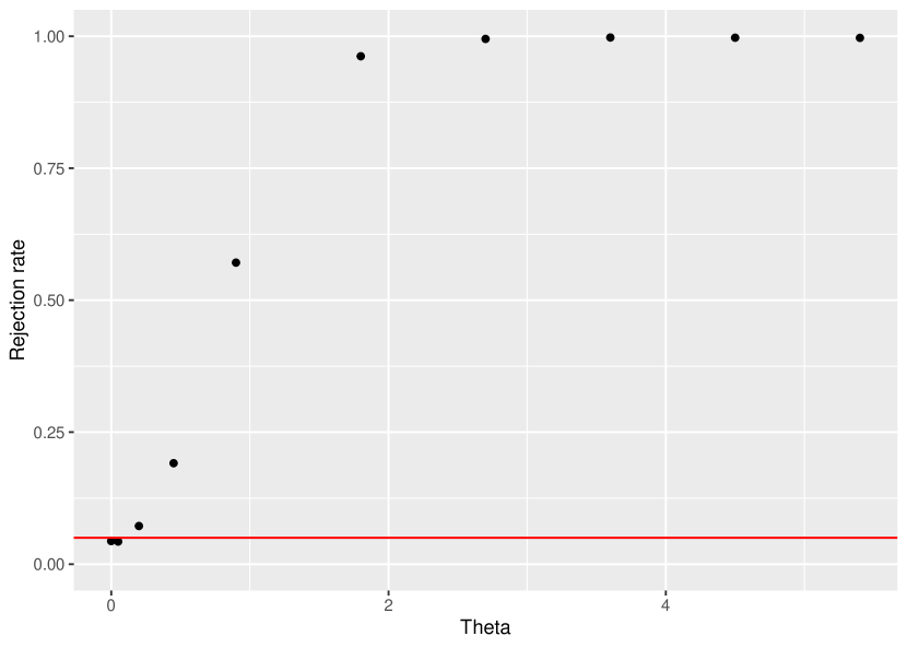
(a) i) Normal

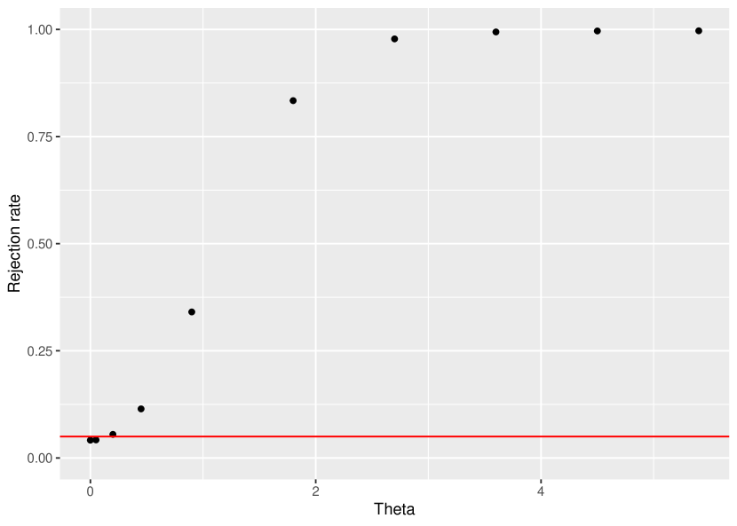
(b) ii) Heteroskedasticity

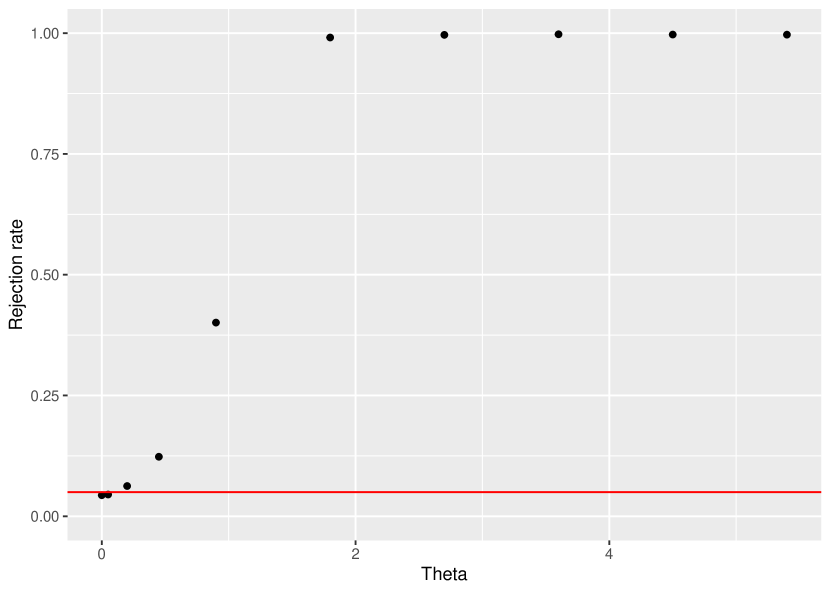
(c) iii) Uniform

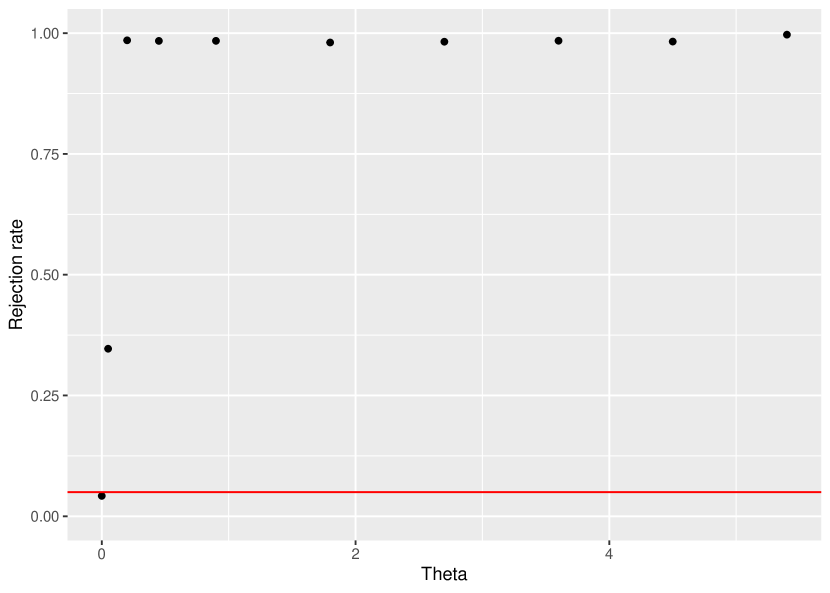
(d) iv) Fat tails

In order to gain intuition regarding this last fact and the magnitude of $\theta_{1}$ observe that the moment for the treated units is given by $(\sum_{i=1}^{n}D_{i})^{-1}\sum_{i=1}^{n}D_{i}(1\{U_{i}/\sigma_{U}\leq(\hat{\theta}_{0}-\theta_{0})/\sigma_{U}-\theta_{1}/\sigma_{U}\}-0.5)$, where $\hat{\theta}_{0}$ is the estimator — computed using the moment for the control units — of $\theta_{0}$. Roughly speaking, $(\hat{\theta}_{0}-\theta_{0})/\sigma_{U}\approx 1/(n-\sum_{i=1}^{n}D_{i})^{0.5}\approx 1/n^{0.5}$, thus for values of $\theta_{1}/\sigma_{U}$ in the range $[0,n^{-1/2}]\approx[0,0.07]$ the power function is expected to be close to 0 and without an specific shape. For values of $\theta_{1}/\sigma_{U}$ in the range $[n^{-1/2},(\sum_{i=1}^{n}D_{i})^{-1/2}]$ (which is approximately given by $[0.07,0.35]$) the power function is expected to be increasing, but not necessarily far from 0 as the deviations of the null are of smaller order than the variability of the moment. Hence, we expect our test to have non-trivial power only for deviations that are larger than $(\sum_{i=1}^{n}D_{i})^{-1/2}\approx 0.35$. Moreover, how fast the power function increases it depends on the variability of $U_{i}/\sigma_{U}$, this heterogeneity among the different models is depicted in Figure 1.

We conclude by pointing out that while this is an apt description of the “average” (across MC repetitions) power function, for particular MC repetitions its behavior can be quite different. In fact, if the number of treated units is “extremely” small our test could reject with, essentially, zero probability and have a power function flat at zero. This feature stems from an “integer problem” in cases where the number of treated units is “extremely” small, rather than from the design of our test. To shed light on this fact lets consider a simplified version of the test statistic: One rejects the null of $\theta_{1}=0$ if $\left|\sum_{i=1}^{n}D_{i}1\{Y_{i}\leq\hat{\theta}_{0}\}/\sum_{i=1}^{n}D_{i}-\tau\right|\geq t(\alpha,(D_{i})_{i=1}^{n})+\delta$ where

$$t(\alpha,(D_{i})_{i=1}^{n})=\min\left\{t\colon\Pr\left(\mathcal{B}(\sum_{i=1}^{n}D_{i})\leq t\right)\geq 1-\alpha\right\}$$

where $\mathcal{B}(\sum_{i=1}^{n}D_{i}):=\left|Bi(\tau,\sum_{i=1}^{n}D_{i})/\sum_{i=1}^{n}D_{i}-\tau\right|$ and $Bi(p,M)$ is a Binomial random variable with probability of success $p$ and number of trials $M$. It turns out that given a $\alpha\in(0,1)$, there exists a cutoff $N_{1}$ such that for any $\sum_{i=1}^{n}D_{i}\leq N_{1}$, $t(\alpha,(D_{i})_{i=1}^{n})$ will equal the highest value in the support of $\mathcal{B}(\sum_{i=1}^{n}D_{i})$, and hence, the highest value in the support of $\left|\sum_{i=1}^{n}D_{i}1\{Y_{i}\leq\hat{\theta}_{0}\}/\sum_{i=1}^{n}D_{i}-\tau\right|$ as well. So, for any such number of treated units, our test will reject with probability 0. For the case of $\tau=0.5$ and $\alpha=0.05$, such cutoff number is $5$. Therefore, while our theory indicates the proposed test will not over-reject for any number of units in the treatment groups, the power of the test can, mechanically, be very low in cases where the number of units in the treatment groups is extremely low.

Overall, the MC study shows that for moderate and even small sample sizes our test has rejection rates that are close to nominal ones, although being somewhat conservative for some designs. It also has non-trivial power for deviations of the null that are approximately larger than $(\sum_{i=1}^{n}D_{i})^{-1/2}$. Finally, while our methodology can handle any number of treated units, for extremely low numbers our test will essentially reject with probability zero. This seems to be a feature of the problem rather than an idiosyncratic characteristic of our test.

7 Empirical application: The Effect of Weather on Growth

In this section we apply our method to gauge the effect of large temperature changes on the cross-sectional distribution of GDP growth. We use the data from Dell et al. [2012] and complement their analysis in two directions. First, we study the effect of temperature changes on the 0.25, 0.50 and 0.75 quantiles of GDP growth. Second, we construct treatment profiles that allows us to estimate a saturated model as opposed to the linear regression model used by Dell et al. [2012] and that was presented in Example 1. The purpose of this exercise is to compare the conclusions we obtain from doing inference based on standard asymptotics to what we obtain when using the method proposed in this paper.

More precisely, growth of country $i$ in period $1990-1994$, $Y_{i}$, satisfies the following equation

$$Y_{i}=\kappa+\sum_{l\in\{0,1\}^{4}}\theta_{l}M_{i}(l)+\Lambda^{T}X_{i}+U_{i}$$ (11)

in which $E[1\{U\leq 0\}|M,X]=\tau$ with $\tau\in\{0.25,0.50,0.75\}$ and $M_{i}(l)$ takes value one if the history of weather events $(D_{1990},...,D_{1994})$ for $i$ equals $l$ and 0 otherwise. The variable $D_{i,t}$ is defined as $1$ if the change in temperature in country $i$ between period $t-1$ and period $t$ was larger than one degree Celsius. Following the preferred specification in Dell et al. [2012], $X_{i}$ includes region fixed effects, and the amount of rainfall of country $i$ in 1994. We restrict the sample to countries that are below the median of the GDP distribution in 1950, since those are the countries for which Dell et al. [2012] find significant effect of temperature changes on GDP.

In Table 7 we show the size of each treatment group defined by $(D_{1990},...,D_{1994})$. We can see that the control group, $(0,0,0,0)$, has 49 units whereas the other treatment groups has less, oscillating between 1 to 6 observations. Hence, standard inferential theory based on t-statistics or F-statistics can be unreliable and untrustworthy.

Table 3: Number of observations for each treatment profile

profile	No.
00000	49
00001	6
00011	1
00100	1
10000	4
Total	61

We report the estimated coefficients in Table 4. In column 1 we show that, when estimating the coefficients in 11 by OLS and using standard heterosckedastic robust SE, only contemporaneous temperature seems to matter for growth, i.e., the profile $00001$. The same result holds for quantiles 0.25, 0.5, and 0.75, which we show in columns 2-4. However, when using our method to test the null hypothesis that $\theta_{0001}=0$ we cannot reject it at a $95\%$ level. Moreover, when testing the joint null hypothesis of no effect from any temperature shock during the 1990-1994 period, i.e., $\theta_{0001}=\theta_{00011}=...=\theta_{1000}=0$ we also cannot reject this null.

	(1)	(2)	(3)	(4)
	OLS	$\tau=0.25$	$\tau=0.5$	$\tau=0.75$
Dependent variable: GDP growth
00000	0	0	0	0
	(.)	(.)	(.)	(.)
00001	-7.4${}^{***}$	-7.7${}^{***}$	-11${}^{***}$	-6.4${}^{***}$
	(2.4)	(1.5)	(2.9)	(1.6)
00011	.36	3.9	-2.6	-2.8
	(2.1)	(.)	(.)	(.)
00100	2.6	3.4	.4	-1.4
	(3.3)	(.)	(.)	(.)
10000	5.2	3.6	4.8${}^{**}$	1.7
	(3.5)	(3.2)	(1.9)	(2.6)
Mean of dependent variable in the 00000 group	-.82	-.82	-.82	-.82
Our method indicator for rejection: 00001 group		0	0	0
Our method indicator for rejection: joint hypothesis		0	0	0
This specification does not include country fixed effects
${}^{*}$ $p<0.1$, ${}^{**}$ $p<0.05$, ${}^{***}$ $p<0.01$

Table 4: Estimates of the effect of different profiles of weather shocks in output growth.

Appendix A Extension: Many Calendar Times

One limitation of the theory put forward in the paper is that it fixes a calendar time $t$. This is specially restrictive if one would like to test a hypothesis involving parameters across many time periods. Here we show how to extend our results to cover this case.

Let $\mathcal{T}:=\{t_{1},...,t_{M}\}\subseteq\mathbb{T}$ be the subset of time periods we would like to use. For each $m\in\{1,...,M\}$, fix a $x^{t_{m}}$, $d^{t_{m}}$ and $\tau_{t_{m}}:=\tau_{m}\in(0,1)$. Then, the null hypothesis is of the form

$$H_{0}\leavevmode\nobreak\ :\leavevmode\nobreak\ \mu_{t}(\cdot,x^{t},d^{t},\tau_{t})=\mu_{t}(\cdot,x^{t},0^{t},\tau_{t}),\leavevmode\nobreak\ \forall t\in\mathcal{T}.$$

Remark 7.

We only present simple hypothesis to simplify the exposition; it is straightforward to extend the results in this section to allow for joint hypothesis simply by following the steps in the paper. $\triangle$

We now introduce some notation. Let μ(y^t_M-1 ,x^t_M,d^t_M,τ) : = (μ_t_1(y^t_1-1, x^t_1,d^t_1,τ_1) ,…, μ_t_M(y^t_M-1, x^t_M,d^t_M,τ_M)), $\boldsymbol{K}:=(K_{1},...,K_{M})$, and $\boldsymbol{m}_{n,\boldsymbol{K}}(x^{t_{M}},\delta^{t_{M}},\boldsymbol{h},P):=m_{K_{1}}(x^{t_{1}},\delta^{t_{1}},h_{1},P),...,m_{K_{M}}(x^{t_{M}},\delta^{t_{M}},h_{M},P)$, where the moment function $m_{K}$ is now defined as

$$m_{K_{m}}(x^{t_{m}},\delta^{t_{m}},h_{m},P):=E_{P}[(\rho(Y_{t_{m}},h_{m}(Y^{t_{m}-1}))-\tau)\Phi_{K_{m}}(Y^{t_{1}-1})\mid(X^{t_{m}},D^{t_{m}})=(x^{t_{m}},\delta^{t_{m}})]$$

Assumption 7.

(i) $(U_{t_{1}}(d^{t_{1}}),...,U_{t_{M}}(d^{t_{M}}))$ are independent conditional on $(Y^{t_{1}-1},X^{t_{M}},D^{t_{M}})$; (ii) for any $m\in\{1,...,M\}$ and any $d^{t_{m}}$, $P\left(U_{t_{m}}(d^{t_{m}})\leq\tau_{m}\mid Y^{t_{1}},D^{t_{M}},X^{t_{M}}\right)=\tau_{m}$.

Remark 8 (Remark about the assumption).

Part (i) is relatively mild and it is satisfied if the $U$’s are independent across time.

Part (ii) of this assumption essentially requires a sort of “strict exogeneity” restriction with respect to $X,D$, e.g. $U_{t}$ is independent of the past, current and future $(X,D)$, and, with respect to $Y$, requires a “sequential exogeneity” type restriction. $\triangle$

The following lemma is analogous to Lemma 1 and is key to establish the asymptotic distribution of our test statistic for this case of many time periods.

Lemma 2.

Suppose Assumptions 1, 2 and 7 hold. Then, for any $(n,\boldsymbol{K})\in\mathbb{N}^{M+1}$ and any $\delta^{t_{M}}\in\{0^{t_{M}},d^{t_{M}}\}$, under the null hypothesis, conditionally on $(Y^{t_{1}-1}_{i},X^{t_{M}}_{i},D^{t_{M}}_{i})_{i=1}^{n}$, the vector $\boldsymbol{m}_{n,\boldsymbol{K}}(x^{t_{M}},\delta^{t_{M}},\boldsymbol{\mu}(\cdot,x^{t_{M}},0^{t_{M}},\boldsymbol{\tau}),P_{n})$ has the same distribution as $\boldsymbol{\ell}_{n,\boldsymbol{K}}:=(\ell_{n,K_{1}}[1],...,\ell_{n,K_{M}}[M])$ where, for any $m\in\{1,...,M\}$,

$$\ell_{n,K_{m}}[m]:=\frac{1}{|\mathcal{G}_{n}(x^{t_{m}},\delta^{t_{m}})|}\sum_{i\in\mathcal{G}_{n}(x^{t_{m}},\delta^{t_{m}})}(B_{i}[m]-\tau)\Phi_{K}(Y^{t_{1}-1}_{i})$$

where for each $(i,m)$, $B_{i}[m]$ are IID drawn from $Ber(\tau_{m})$.

Proof of Lemma 2.

Let $\mathcal{G}_{n}[m]:=\mathcal{G}_{n}(x^{t_{m}},d^{t_{m}})$. Under the null hypothesis, $\mu(x^{t_{m}},d^{t_{m}},\tau_{m})=\mu(x^{t_{m}},0^{t_{m}},\tau_{m})$ for any $m\in\{1,...,M\}$, so

$$\frac{1}{|\mathcal{G}_{n}[m]|}\sum_{i\in\mathcal{G}_{n}[m]}(\rho(Y_{i,t_{m}},\mu(Y^{t_{m}-1}_{i},x^{t_{m}},0^{t_{m}},\tau_{m})))-\tau_{m})\Phi_{K_{m}}(Y^{t_{1}-1}_{i})$$

$$= \frac{1}{|\mathcal{G}_{n}[m]|}\sum_{i\in\mathcal{G}_{n}[m]}(\rho(Y_{i,t_{m}},\mu(Y^{t_{m}-1}_{i},x^{t_{m}},d^{t_{m}},\tau_{m}))-\tau_{m})\Phi_{K_{m}}(Y^{t_{1}-1}_{i})$$

$$= \frac{1}{|\mathcal{G}_{n}[m]|}\sum_{i=1}^{n}1\{(X^{t_{m}}_{i},D^{t_{m}}_{i})=(x^{t_{m}},d^{t_{m}})\}(1\{U_{i,t}(d^{t_{m}})\leq\tau_{m}\}-\tau_{m})\Phi_{K_{m}}(Y^{t_{1}-1}_{i}),$$

where the last line follows from Assumption 2. Hence, we need to study the distribution of this last expression, conditional on $(X^{t_{M}}_{i},D^{t_{M}}_{i},Y^{t_{1}-1}_{i})_{i=1}^{n}$. The only source of randomness is $1\{U_{i,t_{m}}(d^{t_{m}})\leq\tau_{m}\}$ for $i$. By Assumption 1, these are independent random variables; moreover, for any $u_{1},...,u_{M}\in\{0,1\}^{M}$,

$$P\left(1\{U_{i,t_{1}}(d^{t_{1}})\leq\tau_{1}\}=u_{1},...,1\{U_{i,t_{M}}(d^{t_{M}})\leq\tau_{M}\}=u_{M}\mid Y^{t_{1}-1}_{i},D^{t_{M}}_{i},X^{t_{M}}_{i}\right)$$

$$= P\left(1\{U_{t_{1}}(d^{t_{1}})\leq\tau_{1}\}=u_{1},...,1\{U_{t_{M}}(d^{t_{M}})\leq\tau_{M}\}=u_{M}\mid Y^{t_{1}-1},D^{t_{M}},X^{t_{M}}\right)$$

$$= P\left(1\{U_{t_{1}}(d^{t_{1}})\leq\tau_{1}\}=u_{1}\mid Y^{t_{1}-1},D^{t_{M}},X^{t_{M}}\right)\times...\times P\left(1\{U_{t_{M}}(d^{t_{M}})\leq\tau[M]\}=u_{M}\mid Y^{t_{1}-1},D^{t_{M}},X^{t_{M}}\right)$$

$$= \tau_{1}^{u_{1}}(1-\tau_{1})^{1-u_{1}}...\tau_{M}^{u_{M}}(1-\tau_{M})^{1-u_{M}}$$

where the second equality follows because by Assumption 7(i), $U_{t_{1}}(d^{t_{1}}),...,U_{t_{M}}(d^{t_{M}})$ are independent given $(Y^{t_{1}-1},D^{t_{M}},X^{t_{M}})$; the third equality follows from Assumption 7(ii) that states $P\left(U_{t_{m}}(d^{t_{m}})\leq\tau_{m}\mid Y^{t_{1}-1},D^{t_{M}},X^{t_{M}}\right)=\tau_{m}$ for any $m$.

Hence, $(1\{U_{i,t_{m}}(d^{t_{m}})\leq\tau_{m}\})_{i,m}$ are independent Bernoulli random variables with success probability $\tau_{m}$. ∎

This lemma readily implies that

$$\boldsymbol{m}_{n,\boldsymbol{K}}(x^{t_{M}},\delta^{t_{M}},\boldsymbol{\mu}(\cdot,x^{t_{M}},0^{t_{M}},\boldsymbol{\tau}),P_{n})^{\prime}\boldsymbol{m}_{n,\boldsymbol{K}}(x^{t_{M}},\delta^{t_{M}},\boldsymbol{\mu}(\cdot,x^{t_{M}},0^{t_{M}},\boldsymbol{\tau}),P_{n})$$

has the same distribution as

$$\boldsymbol{\ell}_{n,\boldsymbol{K}}^{\prime}\boldsymbol{\ell}_{n,\boldsymbol{K}}.$$

conditional on $(Y^{t_{1}-1}_{i},X^{t_{M}}_{i},D^{t_{M}}_{i})_{i=1}^{n}$. The main result follows by extending assumptions 5 and 6 to the setup with many time periods. However, as the time periods are finite, these extensions do not represent a big qualitative leap from the current assumptions.

Appendix B Appendix for Section 4

We now introduce some notation. Let, $G^{t}:=(X^{t},D^{t})$, $d^{t}[0]:=0^{t}$ and for any $l\in\{0,1,...,M\}$, $\mathcal{T}_{n}[l]:=\mathcal{G}_{n}(x^{t},d^{t}[l])$; this sets keep track of the units in the “control” and “treatment” groups in $\mathcal{D}^{t}$, respectively. For each $i\in\mathbb{N}$, let $\omega_{i}:=(Y_{i,t},O^{t}_{i})=(Y^{t}_{i},G^{t}_{i})$, and $\boldsymbol{\omega}_{\mathcal{T}_{n}[l]}:=\{\omega_{i}\colon i\in\mathcal{T}_{n}[l]\}$. That is, this quantity keeps track of the data associated to the control group and treatments groups, respectively.

In order to ease the notational burden, we omit $(0^{t},x^{t},\tau)$ from the $\mu$. Observe that the estimator for $y^{t-1}\mapsto\mu(y^{t-1})$, $y^{t-1}\mapsto\hat{\mu}_{n,K}(y^{t-1})$, is measurable with respect to $\boldsymbol{\omega}_{\mathcal{T}_{n}[0]}$. In some instances in the proofs it will be useful to make this dependence explicit and we will do so using $\hat{\mu}_{n,K}[\boldsymbol{\omega}_{\mathcal{T}_{n}[0]}]$.

For each $l\in\{0,1,...,M\}$, let $P_{n}[l]$ to be the empirical probability based on the data $\omega_{\mathcal{T}_{n}[l]}$, i.e., $P_{n}[l](A):=|\mathcal{T}_{n}[l]|^{-1}\sum_{i=1}^{n}1\{G^{t}_{i}=(x^{t}_{i},d^{t}[l])\}1\{(Y^{t}_{i},X^{t}_{i},D^{t}_{i})\in A\}$ for any Borel set $A$. Notice that $Q_{K_{l}}(x^{t},d^{t}[l],g,P_{n})$ (and the corresponding estimator) only depends on $P_{n}[l]$; we will sometimes make this explicit by using $Q_{K}(x^{t},d^{t},g,P_{n}[l])$.

Finally, we also use $\rho_{i}(g):=\rho(Y^{t}_{i},X^{t}_{i},d^{t},g)$.

B.1 Proofs for Results in Section 4.1

The following lemma is an adaption of the main theorem in Chernozhukov and Hansen [2005] to our framework, it relates the outcome function, $\mu_{t}$ with the conditional quantile function of $Y_{t}$ given other observables.

Lemma 3.

Suppose Assumptions 2 and 3 hold. Then, for any $t\in\mathbb{T}$ and any $(x^{t},d^{t})\in\mathbb{X}^{t}\times\{0,1\}^{t}$,

$$E[1\{Y_{t}\leq\mu_{t}(Y^{t-1},x^{t},d^{t},\tau)\}\mid Y^{t-1},X^{t}=x^{t},D^{t}=d^{t}]=\tau$$

Proof of Lemma 3.

Under expression 3,

$$Y_{t}(d^{t})=\mu_{t}(Y^{t-1}(d^{t-1}),X^{t},d^{t},U_{t}(d^{t})).$$

So, under Assumption 2, $\{Y_{t}\leq\mu_{t}(Y^{t-1}(d^{t-1}),X^{t},d^{t},\tau)\}=\{U_{t}(d^{t})\leq\tau\}$. Then, under Assumption 3, it follows that for any $d^{t}\in\{0,1\}^{t}$,

$$E[1\{Y_{t}\leq\mu_{t}(Y^{t-1},x^{t},d^{t},\tau)\}\mid Y^{t-1},X^{t}=x^{t},D^{t}=d^{t}]$$

$$= E[1\{U_{t}(d^{t})\leq\tau\}\mid Y^{t-1},X^{t}=x^{t},D^{t}=d^{t}]$$

$$= \tau.$$

This result and LIE deliver the desired result. ∎

Proposition 3.

Suppose Assumption 1 holds and that $\mathcal{H}\subseteq\mathcal{C}^{\upsilon}_{2}(\mathbb{R})$ with $\upsilon>0.5/\delta$, then

$$\sup_{f\in\mathcal{M}_{K_{0}(n)}(0^{t})}|n^{-1}\sum_{i=1}^{n}1\{D^{t}_{i}=0^{t}\}f(Y_{i,t},Y^{t-1}_{i})-E[1\{D^{t}=0^{t}\}f(Y_{t},Y^{t-1})]|=o_{P}(n^{-1/2}\log\log n).$$

for any $(K_{0}(n))_{n}$.

Proof of Proposition 3.

The following calculations are based on the results by Chen et al. [2003] (henceforth, CvKL) and are here mainly for exposition.

Henceforth, we omit $0^{t}$ from the $\mathcal{M}_{K}$ and the like. We first show that

$$\mathcal{I}_{K}\subseteq\mathcal{I}:=\{(d^{t},y^{t})\mapsto 1\{d^{t}=0\}f(y_{t},y^{t-1})\colon f\in\bar{\mathcal{M}}\}$$

where $\mathcal{I}_{K}:=\{(d^{t},y^{t})\mapsto 1\{d^{t}=0\}f(y_{t},y^{t-1})\colon f\in\mathcal{M}_{K}\}$ and

$$\bar{\mathcal{M}}:=\left\{y^{t}\mapsto 1\{y_{t}\leq b+\sum_{s=1}^{P}\gamma_{s}y_{t-s}+g(y_{t-1})\}\colon(b,(\gamma_{s})_{s=1}^{P},g)\in\mathcal{B}\times\mathcal{C}^{\upsilon}_{2}(\mathbb{R})\right\}.$$

And also, that

$$\int\sqrt{\log N_{[]}\left(\iota,\mathcal{I},||.||_{L^{2}(P)}\right)}d\iota<\infty,$$

where $N_{[]}$ is the bracketing number of $\mathcal{I}$, we refer the reader to CvKL for a formal definition.

The set inclusion follows because $\mathcal{H}$ belongs to the $\mathcal{C}^{\upsilon}_{2}(\mathbb{R})$ class by assumption. We now show the bound on the bracketing number $N_{[]}$. In what follows, let $\lambda:=(b,(\gamma_{s})_{s=1}^{P})$. Let $(\lambda_{l})_{l=1}^{L(\eta)}$ be an $\eta$-cover of $(\mathcal{B},||.||)$ and let $(g_{l})_{l=1}^{L(\eta)}$ be an $\eta$-cover of $(\mathcal{C}^{\upsilon}_{2}(\mathbb{R}),||.||_{L^{\infty}})$. Hence, for any $f\in\bar{\mathcal{M}}$, there exist a $l_{1}$ and $l_{2}$ such that, for all $y^{t-1}$,

$$1\{d^{t}=0\}\underline{f}_{l_{1},l_{2},\eta}(y^{t})\leq 1\{d^{t}=0\}f(y^{t})\leq 1\{d^{t}=0\}\bar{f}_{l_{1},l_{2},\eta}(y^{t}).$$

where $\bar{f}_{l_{1},l_{2},\eta}(y^{t}):=1\{y_{t}\leq b_{l_{1}}+\sum_{s=1}^{P}\gamma_{l_{1},s}y_{t-s}+g_{l_{2}}(y_{t-1})+\eta\}$ and $\underline{f}_{l_{1},l_{2},\eta}(y^{t}):=1\{y_{t}\leq b_{l_{1}}+\sum_{s=1}^{P}\gamma_{l_{1},s}y_{t-s}+g_{l_{2}}(y_{t-1})-\eta\}$. Moreover,

$$||1\{\cdot=0^{t}\}(\underline{f}_{l_{1},l_{2},\eta}-\bar{f}_{l_{1},l_{2},\eta})||^{2}_{L^{2}(P)}\leq ||\underline{f}_{l_{1},l_{2},\eta}-\bar{f}_{l_{1},l_{2},\eta}||^{2}_{L^{2}(P)}$$

$$\leq E[(F(H(Y^{t-1})+\eta\mid Y^{t-1})-F(H(Y^{t-1})-\eta\mid Y^{t-1}))]$$

$$\leq A(2\eta)^{\delta}.$$

where $H(y^{t-1}):=b_{l_{1}}+\sum_{s=1}^{P}\gamma_{l_{1},s}y_{t-s}+g_{l_{2}}(y_{t-1})$; and where the last line follows because $F(.|D^{t},Y^{t-1})$ it is assumed to be Hölder with parameter $(A,\delta)$. This shows that $[1\{\cdot=0^{t}\}\underline{f}_{l_{1},l_{2},\eta},1\{\cdot=0^{t}\}\bar{f}_{l_{1},l_{2},\eta}]$ for all $(l_{1},l_{2})\in\{1,...,L(\eta)\}^{2}$ form $\iota:=A(2\eta)^{\delta}$-brackets for $(\mathcal{I},L^{2}(P))$.

This in turn implies that for all $K$,

$$N_{[]}\left(\iota,\mathcal{I}_{K},||.||_{L^{2}(P)}\right)\leq N_{[]}\left(\iota,\mathcal{I},||.||_{L^{2}(P)}\right)$$

$$\leq N\left((\iota/A)^{1/\delta},\mathcal{B},||.||\right)\times N\left((\iota/A)^{1/\delta},\mathcal{C}^{\alpha}_{2}(\mathbb{R}),||.||_{L^{\infty}}\right)$$

Since $\mathcal{B}$ is compact, it follows that $\int\sqrt{\log N\left((\iota/A)^{1/\delta},\mathcal{B},||.||\right)}d\iota<\infty$. By Van Der Vaart et al. [1996], for any $\epsilon>0$, $N\left(\epsilon,\mathcal{C}^{\upsilon}_{2}(\mathbb{R}),||.||_{L^{\infty}}\right)\leq(1/\epsilon)^{1/\upsilon}\sum_{j=1}^{\infty}P(R_{j})$ where $(R_{j})_{j}$ is any partition of $\mathbb{R}$ of bounded sets. Since there exists a partition such that $\sum_{j=1}^{\infty}P(R_{j})<\infty$, it follows that $N\left(\epsilon^{1/\delta},\mathcal{C}^{\upsilon}_{2}(\mathbb{R}),||.||_{L^{\infty}}\right)\leq(1/\epsilon)^{1/(\delta\upsilon)}$. Thus, $\int\sqrt{\log N\left((\iota/A)^{1/\delta},\mathcal{C}^{\upsilon}_{2}(\mathbb{R}),||.||_{L^{\infty}}\right)}d\iota<\infty$ provided $\upsilon>1/(2\delta)$. Therefore, the desired result holds.

Observe that for any $(K_{0}(n))_{n}$,

$$\sup_{f\in\mathcal{M}_{K_{0}(n)}}|n^{-1}\sum_{i=1}^{n}1\{D^{t}_{i}=0^{t}\}f(Y_{i,t},Y^{t-1}_{i})-E[1\{D^{t}=0^{t}\}f(Y_{t},Y^{t-1})]|$$

$$\leq \sup_{g\in\mathcal{I}}|n^{-1}\sum_{i=1}^{n}g(D^{t}_{i},Y^{t}_{i})-E[g(D^{t},Y^{t})]|$$

so it suffices to bound the quantity on the RHS. Since $\int\sqrt{\log N_{[]}\left(\iota,\mathcal{I},||.||_{L^{2}(P)}\right)}d\iota<\infty$ and any element in $\mathcal{I}$ is bounded, it follows by the results in Van Der Vaart et al. [1996] that

$$\sup_{g\in\mathcal{I}}|n^{-1}\sum_{i=1}^{n}g(D^{t}_{i},Y^{t}_{i})-E[g(D^{t},Y^{t})]|=O_{P}(n^{-1/2}),$$

hence $\varrho_{n}$ can be taken to be $l_{n}n^{-1/2}$ for any slowly diverging sequence $(l_{n})_{n}$. ∎

B.2 Proof for Results in Section 4.2

Proof of Lemma 1.

Under the null hypothesis, $\mu(x^{t},0^{t},\tau)=\mu(x^{t},\delta^{t},\tau)$ for any $\delta^{t}\in\mathcal{D}^{t}$, so

$$\frac{1}{|\mathcal{G}_{n}(x^{t},\delta^{t})|}\sum_{i\in\mathcal{G}_{n}(x^{t},\delta^{t})}(\rho(Y_{i,t},\mu(Y^{t-1}_{i},x^{t}),0^{t},\tau))-\tau)\Phi_{K}(Y^{t-1}_{i})$$

$$= \frac{1}{|\mathcal{G}_{n}(x^{t},\delta^{t})|}\sum_{i\in\mathcal{G}_{n}(x^{t},\delta^{t})}(\rho(Y_{i,t},\mu(Y^{t-1}_{i},x^{t}),\delta^{t},\tau))-\tau)\Phi_{K}(Y^{t-1}_{i})$$

$$= \frac{1}{|\mathcal{G}_{n}(x^{t},\delta^{t})|}\sum_{i=1}^{n}1\{(X^{t}_{i},D^{t}_{i})=(x^{t},\delta^{t})\}(1\{U_{i,t}(\delta^{t})\leq\tau\}-\tau)\Phi_{K}(Y^{t-1}_{i}),$$

where the last line follows from Assumption 2. Hence, we need to study the distribution of this last expression, conditional on $(X^{t}_{i},D^{t}_{i},Y^{t-1}_{i})_{i=1}^{n}$. The only source of randomness is the vector $(1\{U_{i,t}(\delta^{t})\leq\tau\})_{i\in\mathcal{G}_{n}(x^{t},\delta^{t})}$. By Assumption 1, these are independent random variables; moreover,

$$P\left(1\{U_{i,t}(\delta^{t})\leq\tau\}=1\mid Y^{t-1}_{i},(D^{t}_{i},X^{t}_{i})=(\delta^{t},x^{t})\right)$$

$$= P\left(1\{U_{t}(\delta^{t})\leq\tau\}=1\mid Y^{t-1},(D^{t},X^{t})=(\delta^{t},x^{t})\right)$$

$$= P\left(U_{t}(\delta^{t})\leq\tau\mid Y^{t-1},(D^{t},X^{t})=(\delta^{t},x^{t})\right)=\tau$$

where the last equality follows from Assumption 3. Hence, $1\{U_{t}(\delta^{t})\leq\tau\}\sim Ber(\tau)$ given $Y^{t-1},(D^{t},X^{t})=(\delta^{t},x^{t})$. ∎

B.2.1 Proof of Theorem 1

In order to show Theorem 1 we first establish a series of lemmas whose proofs are relegated to the end of this appendix.

The following Lemma provides a quantitative bound for “$o_{P}$” statements.

Lemma 4.

Suppose $X_{n}=o_{P}(1)$, then there exists a $(\epsilon_{n})_{n}$ such that $(\epsilon_{n})_{n}$ is non-increasing and converges to $0$, and

$$P(X_{n}\geq\epsilon_{n})\leq\epsilon_{n}$$

for all $n$.

The next lemma establishes an approximation result for Laws that allow for discontinuous random variables, as it is the case for $\mathcal{B}_{n,K}$.

Lemma 5.

Let $(A_{n})_{n}$, $(B_{n})_{n}$ and $(C_{n})_{n}$ be a sequence of real-valued random variables, suppose there exists sequences positive-valued sequences $(r_{n},\epsilon_{n})_{n}$ such that $\epsilon_{n}=o(1)$, $\liminf_{n\rightarrow\infty}r_{n}\geq 1$ and

$$\Pr(r_{n}|A_{n}-B_{n}|\geq\epsilon_{n})\leq\epsilon_{n}$$ (12)

for all $n$. Then,

$$\liminf_{n\rightarrow\infty}\Pr\left(\sup_{t}\Pr(r_{n}A_{n}\geq t+\delta\mid C_{n})-\Pr(r_{n}B_{n}\geq t\mid C_{n})\leq\sqrt{\epsilon_{n}}\right)=1.$$

We use this lemma to show Theorem 1 by taking, for each $l\in\{1,...,M\}$, $A_{n}:=Q_{K_{l}(n)}(x^{t},d^{t}[l],\hat{\mu}_{n,K_{0}(n)},P_{n})$ and $B_{n}:=Q_{K_{l}(n)}(x^{t},d^{t}[l],\mu,P_{n})$. To do this, is crucial to verify condition 12 in the Lemma. The next lemma provides sufficient conditions and an explicit expression for $(r_{n})_{n}$. In what follows, let $q$ be some number in $[1,\infty]$ and

$$S_{n}(\eta_{n}):=\{\boldsymbol{\omega}_{\mathcal{T}_{n}[0]}\colon\max_{d^{t}\in\mathcal{D}^{t}\cup\{0^{t}\}}||\hat{\mu}_{n,K_{0}(n)}[\boldsymbol{\omega}_{\mathcal{T}_{n}[0]}]-\mu||_{L^{q\delta}(P(\cdot|(x^{t},d^{t})))}\leq\eta_{n}\},$$

where $(\eta_{n})_{n}$ is any real-valued sequence.

Lemma 6.

Suppose Assumptions 1 and 4 hold, and the following conditions hold:

1. For any $n$, there exists a $\epsilon>0$ such that $P(S_{n}(\eta_{n}))\geq 1-\epsilon$.

2. There exists a positive real-valued sequences, $(\varrho_{n})_{n}$ and $(K_{0}(n))_{n}$, such that $\varrho_{n}=o(1)$ and

   $$\|\sup_{f\in\mathcal{M}_{K_{0}(n)}(0^{t})}n^{-1}\sum_{i=1}^{n}1\{G_{i}=(x^{t},0^{t})\}\{f(Y_{t,i},Y^{t-1}_{i})-E_{P}[f(Y_{t},Y^{t-1})\mid G_{i}=(x^{t},0^{t})]\}\|^{2}=o_{P}(\varrho_{n}),$$

   where

   $$\mathcal{M}_{K_{0}(n)}(0^{t}):=\left\{(y_{t},y^{t-1})\mapsto(1\{y_{t}\leq h(y^{t-1})\}-1\{y_{t}\leq\mu(y^{t-1})\})\Phi_{K_{0}(n)}(y^{t-1})\colon h\in\mathbb{H}_{K_{0}(n)}(0^{t})\right\}.$$

Then, there exists a $N$ and a constant $C>0$ such that, for any $q^{\prime}$ is such that $1/q^{\prime}+1/q=1$ and any $n\geq N$,

$$P\left(|Q_{\mathbf{K}(n)}(x^{t},\hat{\mu}_{n,K_{0}(n)},P_{n})-Q_{\mathbf{K}(n)}(x^{t},\mu,P_{n})|\geq Cr^{2}_{n}(\epsilon,\mathbf{K}(n))+2Cb_{n}(\mathbf{K}(n))\times r_{n}(\epsilon,\mathbf{K}(n))\right)\leq 4\epsilon,$$

where $\mathbf{K}(n):=(K_{0}(n),K_{1},...,K_{M})$ and

$$r_{n}(\epsilon,\mathbf{K}(n)):= M\times\sqrt{2\epsilon\max_{l\in\{1,...,M\}}||\Phi_{K_{l}}||^{2}_{L^{2}(P(\cdot|(x^{t},d^{t}[l])))}+\eta_{n}^{\delta}\max_{l\in\{1,...,M\}}||A||\Phi_{K_{l}}||^{2}||_{L^{q^{\prime}}(P(\cdot\mid(x^{t},d^{t}[l])))}}$$

$$+\sqrt{\varrho_{n}+\eta_{n}^{\delta}||A||\Phi_{K_{0}(n)}||^{2}||_{L^{q^{\prime}}(P(.\mid(x^{t},d^{t}[0])))}}.$$

and

$$b_{n}(\mathbf{K}(n)):=M\max_{l\in\{1,...,M\}}||\Phi_{K_{l}}||_{L^{2}(P(\cdot\mid x^{t},d^{t}[l]))}+||\Phi_{K_{0}(n)}||_{L^{2}(P(\cdot\mid x^{t},d^{t}[0]))}$$

We can now prove Theorem 1.

Proof of Theorem 1.

Let

$$rate_{n}:=1/((r^{2}_{n}(\varpi^{-1}_{n},\mathbf{K}(n))+2b_{n}(\mathbf{K}(n))\times r_{n}(\varpi^{-1}_{n},\mathbf{K}(n)))$$

where $r_{n}$ and $b_{n}$ are as in Lemma 6. Note that under Assumption 5, $\lim_{n\rightarrow\infty}rate_{n}=\infty$.

In this proof we will actually show a stronger statement that then one in the theorem. We will show that for any $(l_{n},s_{n})_{n}$ such that $l^{-1}_{n}=o(1)$, $\liminf_{n\rightarrow\infty}s_{n}>0$, $\lim_{n\rightarrow\infty}\frac{rate_{n}}{l_{n}s_{n}}=\infty$ and any $\delta>0$,

$$\limsup_{n\rightarrow\infty}E_{P}[1\{s_{n}Q_{\mathbf{K}(n)}(x^{t},\hat{\mu}_{n,K_{0}(n)}(\cdot,x^{t},0^{t},\tau),P_{n})\geq t_{\mathbf{K}(n)}(\alpha,(O^{t}_{i})_{i=1}^{n})+\delta\}]\leq\alpha$$

where — abusing notation — $t_{\mathbf{K}(n)}(\alpha,(O^{t}_{i})_{i=1}^{n})$ is defined by

$$t_{\mathbf{K}(n)}(\alpha,(O^{t}_{i})_{i=1}^{n}):=\inf\{t\colon\Pr(s_{n}\mathcal{B}_{n,\mathbf{K}(n)}\leq t\mid(O^{t}_{i})_{i=1}^{n})\geq\alpha\}.$$

It is clear that this statement implies Theorem 1 provided $s_{n}=1$ for all $n$. Because $\lim_{n\rightarrow\infty}rate_{n}=\infty$ by Assumption 5(ii), there always exists a diverging sequence $(l_{n})_{n}$ such that $\lim_{n\rightarrow\infty}rate_{n}/l_{n}=\infty$; hence $s_{n}=1$ for all $n$ is indeed a valid choice.

We first show that our assumptions imply the conditions in Lemma 6 for large $n$. Assumptions 1 and 4 are directly imposed; Assumption 5 implies condition 1 with $\eta_{n}$ and $q$ equal to the one in the assumption and $\epsilon=\varpi^{-1}_{n}$; and Assumption 6 implies condition 2. Therefore, for any $\epsilon>0$, there exists a $N$ such that for all $n\geq N$,

$$P\left(rate_{n}|Q_{\mathbf{K}(n)}(x^{t},\hat{\mu}_{n,K_{0}(n)},P_{n})-Q_{\mathbf{K}(n)}(x^{t},\mu,P_{n})|\leq l_{n}\epsilon\right)\geq 1-\epsilon$$

Let $(s_{n})_{n}$ be any sequence satisfying the restrictions at the beginning of the proof; such sequence exists as $rate_{n}$ diverges. It readily follows that

$$P\left(s_{n}|Q_{\mathbf{K}(n)}(x^{t},\hat{\mu}_{n,K_{0}(n)},P_{n})-Q_{\mathbf{K}(n)}(x^{t},\mu,P_{n})|\leq\epsilon\right)\geq 1-\epsilon.$$

By applying Lemma 4 with $X_{n}:=s_{n}|Q_{\mathbf{K}(n)}(x^{t},\hat{\mu}_{n,K_{0}(n)},P_{n})-Q_{\mathbf{K}(n)}(x^{t},\mu,P_{n})|$ it follows that there exists a $(\epsilon_{n})_{n}$ such that $\epsilon_{n}=o(1)$ and

$$P\left(s_{n}|Q_{\mathbf{K}(n)}(x^{t},\hat{\mu}_{n,K_{0}(n)},P_{n})-Q_{\mathbf{K}(n)}(x^{t},\mu,P_{n})|\geq\epsilon_{n}\right)\leq\epsilon_{n}.$$

Let $A_{n}:=Q_{\mathbf{K}(n)}(x^{t},\hat{\mu}_{n,K_{0}(n)},P_{n})$ and $B_{n}:=Q_{\mathbf{K}(n)}(x^{t},\mu,P_{n})$. By the previous display, it follows that

$$P(s_{n}|A_{n}-B_{n}|\geq\epsilon_{n})\leq\epsilon_{n}.$$

So, condition 12 in Lemma 5 holds with sequences $(s_{n},\epsilon_{n})_{n}$. Thus, by that lemma with $C_{n}:=(O^{t}_{i})_{i=1}^{n}$ and Lemma 1 — which implies that $t\mapsto P(s_{n}Q_{\mathbf{K}(n)}(x^{t},\mu,P_{n})\geq t\mid(O^{t}_{i})_{i=1}^{n})=\Pr(s_{n}\mathcal{B}_{n,\mathbf{K}(n)}\geq t\mid(O^{t}_{i})_{i=1}^{n})$ — it follows that

$$\liminf_{n\rightarrow\infty}P\left(\mathcal{S}_{n}\right)=1$$

where

$$\mathcal{S}_{n}:=\left\{(O^{t}_{i})_{i=1}^{n}\colon\sup_{t}P(s_{n}Q_{\mathbf{K}(n)}(x^{t},\hat{\mu}_{n,K_{0}(n)},P_{n})\geq t+\delta\mid(O^{t}_{i})_{i=1}^{n})-\Pr(s_{n}\mathcal{B}_{n,\mathbf{K}(n)}\geq t\mid(O^{t}_{i})_{i=1}^{n})\leq\epsilon_{n}\right\}.$$

Hence, for any $\gamma>0$, there exists a $N$ such that for all $n\geq N$,

$$E_{P}[\phi_{\mathbf{K}(n)}(t_{\mathbf{K}(n)}(\alpha,(O^{t}_{i})_{i=1}^{n})+\delta,P_{n})]= E_{P}[\phi_{\mathbf{K}(n)}(t_{\mathbf{K}(n)}(\alpha,(O^{t}_{i})_{i=1}^{n})+\delta,P_{n})|\mathcal{S}_{n}]P(\mathcal{S}_{n})$$

$$+E_{P}[\phi_{\mathbf{K}(n)}(t_{\mathbf{K}(n)}(\alpha,(O^{t}_{i})_{i=1}^{n})+\delta,P_{n})|\mathcal{S}_{n}^{C}]P(\mathcal{S}_{n}^{C})$$

$$\leq E_{P}[\phi_{\mathbf{K}(n)}(t_{\mathbf{K}(n)}(\alpha,(O^{t}_{i})_{i=1}^{n})+\delta,P_{n})|\mathcal{S}_{n}]+\gamma$$

By LIE, $E_{P}[\phi_{\mathbf{K}(n)}(t_{\mathbf{K}(n)}(\alpha,(O^{t}_{i})_{i=1}^{n})+\delta,P_{n})|\mathcal{S}_{n}]=E_{P}[E_{P}[\phi_{\mathbf{K}(n)}(t_{\mathbf{K}(n)}(\alpha,(O^{t}_{i})_{i=1}^{n})+\delta,P_{n})\mid(O^{t}_{i})^{n}_{i=1}]|\mathcal{S}_{n}]$. So it suffices to bound $E_{P}[\phi_{\mathbf{K}(n)}(t_{\mathbf{K}(n)}(\alpha,(O^{t}_{i})_{i=1}^{n})+\delta,P_{n})\mid(O^{t}_{i})^{n}_{i=1}]$ for any $(O^{t})_{i=1}^{n}\in\mathcal{S}_{n}$. To do this, note that for any $(O^{t})_{i=1}^{n}\in\mathcal{S}_{n}$,

$$E_{P}[\phi_{\mathbf{K}(n)}(t_{\mathbf{K}(n)}(\alpha,(O^{t}_{i})_{i=1}^{n})+\delta,P_{n})\mid(O^{t}_{i})^{n}_{i=1}]$$

$$\leq E_{P}\left[1\{s_{n}Q_{\mathbf{K}(n)}(x^{t},\hat{\mu}_{n,K_{0}(n)}(\cdot,x^{t},0^{t},\tau),P_{n})\geq t_{\mathbf{K}(n)}(\alpha,(O^{t}_{i})_{i=1}^{n})+\delta\}\mid(O^{t}_{i})^{n}_{i=1}\right]$$

$$\leq \Pr(s_{n}\mathcal{B}_{n,\mathbf{K}(n)}\geq t_{\mathbf{K}(n)}(\alpha,(O^{t}_{i})_{i=1}^{n})\mid(O^{t}_{i})_{i=1}^{n})+\gamma$$

where the last line follows because $(O^{t})_{i=1}^{n}\in\mathcal{S}_{n}$. Since $\Pr(s_{n}\mathcal{B}_{n,\mathbf{K}(n)}\geq t_{\mathbf{K}(n)}(\alpha,(O^{t}_{i})_{i=1}^{n})\mid(O^{t}_{i})_{i=1}^{n})\leq\alpha$, it follows that for any $\gamma>0$ and any $\delta>0$, there exists a $N$ such that

$$E_{P}[\phi_{\mathbf{K}(n)}(t_{\mathbf{K}(n)}(\alpha,(O^{t}_{i})_{i=1}^{n})+\delta,P_{n})]\leq\alpha+\gamma,\leavevmode\nobreak\ \forall n\geq N.$$

And thus, the desired result holds. ∎

B.2.2 Proofs of Technical Lemmas

Proof of Lemma 4.

$X_{n}=o_{P}(1)$, for any $\epsilon>0$, there exists a $N$ such that

$$P(X_{n}\geq\epsilon)\leq\epsilon$$

for all $n\geq N$.

For each $l\in\mathbb{N}$, let $N_{l}$ be the cutoff above for $\epsilon=1/2^{l}$. WLOG, we can take the sequence $(N_{l})_{l}$ to be increasing. Let $n\mapsto l(n)$ be the mapping such that $n\in\{N_{l(n)},...,N_{l(n)+1}\}$. Clearly this mapping is non-decreasing and diverges as $n$ diverges. To show this last claim, suppose not, then it will imply that there exists a $L$ such that $n\leq N_{L}$ for all $n$, but this is a contradiction.

For each $n$, let $\epsilon_{n}:=1/2^{l(n)}$. As $l(.)$ is non-decreasing and diverging, $(\epsilon_{n})_{n}$ is non-increasing and converges to 0. Also, as $N_{l(n)}$ is such that $n\geq N_{l(n)}$ and thus

$$P(X_{n}\geq 1/2^{l(n)})\leq 1/2^{l(n)}=\epsilon_{n},$$

which clearly implies our result. ∎

Proof of Lemma 5.

Observe that for any $t\in\mathbb{R}$, any real-valued sequence $(\epsilon_{n})_{n}$ and any $n$,

$$\Pr(r_{n}A_{n}\geq t+\delta\mid C_{n})\leq \Pr(\{r_{n}A_{n}\geq t+\delta\}\cap\{r_{n}|A_{n}-B_{n}|<\epsilon_{n}\}\mid C_{n})+\Pr(r_{n}|A_{n}-B_{n}|\geq\epsilon_{n}\mid C_{n})$$

$$\leq \Pr(r_{n}B_{n}\geq t+\delta-\epsilon_{n}\mid C_{n})+\Pr(r_{n}|A_{n}-B_{n}|\geq\epsilon_{n}\mid C_{n})$$

where the second line follows from simple algebra.

By our condition, there exists sequence $(\epsilon_{n})_{n}$ so that $\epsilon_{n}=o(1)$ and $\Pr(r_{n}|A_{n}-B_{n}|\geq\epsilon_{n})\leq\epsilon_{n}$. By our previous calculations and this result, it follows that, for any $\delta>0$ and any $n$,

$$\Pr\left(\sup_{t}\Pr(r_{n}A_{n}\geq t+\delta\mid C_{n})-\Pr(r_{n}B_{n}\geq t+\delta-\epsilon_{n}\mid C_{n})\leq\sqrt{\epsilon_{n}}\right)$$

$$\geq\Pr\left(\Pr(r_{n}|A_{n}-B_{n}|\geq\epsilon_{n}\mid C_{n})\leq\sqrt{\epsilon_{n}}\right).$$

By the Markov inequality and the LIE,

$$\Pr\left(\Pr(r_{n}|A_{n}-B_{n}|\geq\epsilon_{n}\mid C_{n})>\sqrt{\epsilon_{n}}\right)\leq\epsilon^{-1/2}_{n}E[\Pr(r_{n}|A_{n}-B_{n}|\geq\epsilon_{n}\mid C_{n})]=\epsilon^{-1/2}_{n}\Pr(r_{n}|A_{n}-B_{n}|\geq\epsilon_{n}).$$

By our previous results the RHS is equal to $\sqrt{\epsilon_{n}}$. Hence, it follows that

$$\Pr\left(\Pr(r_{n}|A_{n}-B_{n}|\geq\epsilon_{n}\mid C_{n})\leq\sqrt{\epsilon_{n}}\right)\geq 1-\epsilon^{1/2}_{n}.$$

By our choices, the RHS converges to 1. Moreover, since $\epsilon_{n}=o(1)$, it follows that for any $\delta>0$, there exists a $N$ such that

$$\Pr\left(\sup_{t}\Pr(r_{n}A_{n}\geq t+\delta\mid C_{n})-\Pr(r_{n}B_{n}\geq t+\delta-\epsilon_{n}\mid C_{n})\leq\sqrt{\epsilon_{n}}\right)$$

$$\leq \Pr\left(\sup_{t}\Pr(r_{n}A_{n}\geq t+\delta\mid C_{n})-\Pr(r_{n}B_{n}\geq t\mid C_{n})\leq\sqrt{\epsilon_{n}}\right)$$

for all $n\geq N$. Hence,

$$\liminf_{n\rightarrow\infty}\Pr\left(\sup_{t}\Pr(r_{n}A_{n}\geq t+\delta\mid C_{n})-\Pr(r_{n}B_{n}\geq t\mid C_{n})\leq\sqrt{\epsilon_{n}}\right)=1.$$

∎

To show Lemma 6 we need to establish rates of convergence of the (empirical) moment functions for the “treatment” and “control” groups, respectively. We show these separatedly — in Lemmas 8 and 7 below — because the technique of proof for each are very different. In particular, for the moment functions of the “control” group we use uniform convergence of a certain sample average, whereas for the moment functions of the “treatment” group this is not needed. This discrepancy arises from the fact that both moment functions are evaluated in $\hat{\mu}_{n,K_{0}(n)}$ which is independent of the data of the “treatment” group but not for the one of the “control” group.

Recall that $G^{t}:=(X^{t},D^{t})$, i.e., $G^{t}$ is the random variable that defines the group, and to ease the notational burden we omit the superscript $t$, and that

$$S_{n}(\eta_{n}):=\{\boldsymbol{\omega}_{\mathcal{T}_{n}[0]}\colon\max_{d^{t}\in\mathcal{D}^{t}\cup\{0^{t}\}}||\hat{\mu}_{n,K_{0}(n)}[\boldsymbol{\omega}_{\mathcal{T}_{n}[0]}]-\mu||_{L^{q\delta}(P(\cdot|(x^{t},d^{t})))}\leq\eta_{n}\},$$

where $(\eta_{n})_{n}$ is any real-valued sequence. Also, for this lemma, let $F(.|.)$ be the conditional CDF of $Y_{i,t}$ given $(Y^{t-1}_{i},G_{i})$ for any $i\in\mathcal{T}_{n}[0]$.

Lemma 7.

Take any $n\in\mathbb{N}$. Suppose the following conditions holds:

1. There exists a $\epsilon>0$ such that $P(S_{n}(\eta_{n}))\geq 1-\epsilon$.

2. For any $i\in\{1,...,n\}$, $(Y_{i,t},Y^{t-1}_{i},D^{t}_{i})$ are identically distributed and $|\mathcal{G}_{n}(x^{t},0^{t})|/n$ converges to $P(G=(x^{t},0^{t}))>0$, a.s.-$P$.

3. There exists a $y^{t-1}\mapsto A(y^{t-1})$ finite and a $\delta>0$ such that for any $i\in\mathcal{T}_{n}[0]$, $|F(a|Y^{t-1}_{i},G_{i})-F(b|Y^{t-1}_{i},G_{i})|<A(Y^{t-1}_{i})|a-b|^{\delta}$ for any $a,b$.

4. There exists a positive real-valued sequences, $(\varrho_{n})_{n}$ and $(K_{0}(n))_{n}$, such that $\varrho_{n}=o(1)$ and

   $$\|\sup_{f\in\mathcal{M}_{K_{0}(n)}}n^{-1}\sum_{i=1}^{n}1\{G_{i}=(x^{t},0^{t})\}\{f(Y_{t,i},Y^{t-1}_{i})-E_{P}[f(Y_{t},Y^{t-1})\mid G_{i}=(x^{t},0^{t})]\}\|^{2}=o_{P}(\varrho_{n}),$$

   where

   $$\mathcal{M}_{K_{0}(n)}:=\left\{(y_{t},y^{t-1})\mapsto(1\{y_{t}\leq h(y^{t-1})\}-1\{y_{t}\leq\mu(y^{t-1})\})\Phi_{K_{0}(n)}(y^{t-1})\colon h\in\mathbb{H}_{K_{0}(n)}\right\}.$$

Then, there exists a $N$ such that

$$P\left(||m_{K_{0}(n)}(x^{t},0^{t},\hat{\mu}_{n,K_{0}(n)},P_{n})-m_{K_{0}(n)}(x^{t},0^{t},\mu,P_{n})||^{2}\geq\varrho_{n}+\eta_{n}^{\delta}||A||\Phi_{K_{0}(n)}||^{2}||_{L^{q^{\prime}}(P(.\mid(x^{t},0^{t})))}\right)\leq\epsilon$$

for all $n\geq N$ and for any $q^{\prime}$ is such that $1/q^{\prime}+1/q=1$.

Remark 9.

Condition 2 in the Lemma are designed to illustrate what properties of the DGP (summarized in Assumption 1) we need in order to derive convergence rates for the empirical moments of the “control” group. It requires identically distributed random variables so there is only one moment to learn about. The convergence of the frequency to the theoretical probability follows from standard LLN; the assumption that the probability of the “control” group is positive formalizes the intuition that the size of “control” group grows proportionally with the sample size. $\triangle$

Proof of Lemma 7.

For any $i\in\mathbb{N}$, let $g\mapsto\zeta_{i}(g):=(\rho_{i}(g)-\rho_{i}(\mu))\Phi_{K_{0}(n)}(Y^{t-1}_{i})$, note that $\zeta_{i}(g)$ is a random variable measurable with respect to $(Y_{i,t},Y^{t-1}_{i})$. Let $g\mapsto\mathcal{E}_{P}[g\mid G_{i}=(x^{t},0^{t})]:=\int g(y_{t},y^{t-1})P(dy_{t},dy^{t-1}\mid G_{i}=(x^{t},0^{t}))$, importantly, $\mathcal{E}_{P}[\rho_{i}(\hat{\mu}_{n,K_{0}(n)}[\boldsymbol{\omega}_{\mathcal{T}_{n}[0]}])\mid G_{i}=(x^{t},0^{t})]$ is a random variable measurable with respect to $\boldsymbol{\omega}_{\mathcal{T}_{n}[0]}$, but the (implicit) $(Y_{i,t},Y^{t-1}_{i})$ in $\rho_{i}$ and $\hat{\mu}_{n,K_{0}(n)}[\boldsymbol{\omega}_{\mathcal{T}_{n}[0]}]$ are being integrated.

It follows that

$$||m_{K_{0}(n)}(x^{t},0^{t},\hat{\mu}_{n,K_{0}(n)},P_{n})-m_{K_{0}(n)}(x^{t},0^{t},\mu,P_{n})||^{2}$$

$$\leq 2|||\mathcal{T}_{n}[0]|^{-1}\sum_{i=1}^{n}1\{G_{i}=(x^{t},0^{t})\}\{\zeta_{i}(\hat{\mu}_{n,K_{0}(n)}[\boldsymbol{\omega}_{\mathcal{T}_{n}[0]}])-\mathcal{E}_{P}[\zeta_{i}(\hat{\mu}_{n,K_{0}(n)}[\boldsymbol{\omega}_{\mathcal{T}_{n}[0]}])\mid G_{i}=(x^{t},0^{t})]\}||^{2}$$

$$+2|||\mathcal{T}_{n}[0]|^{-1}\sum_{i=1}^{n}1\{G_{i}=(x^{t},0^{t})\}\mathcal{E}_{P}[\zeta_{i}(\hat{\mu}_{n,K_{0}(n)}[\boldsymbol{\omega}_{\mathcal{T}_{n}[0]}])\mid G_{i}=(x^{t},0^{t})]||^{2}$$

$$=:T_{1,n}[\boldsymbol{\omega}_{\mathcal{T}_{n}[0]}]+T_{2,n}[\boldsymbol{\omega}_{\mathcal{T}_{n}[0]}].$$

We will now bound each of the terms in the RHS separately.

It is easy to see that

$$T_{1,n}[\boldsymbol{\omega}_{\mathcal{T}_{n}[0]}]\leq 2\|\sup_{f\in\mathcal{M}_{K_{0}(n)}}|\mathcal{T}_{n}[0]|^{-1}\sum_{i=1}^{n}1\{G_{i}=(x^{t},0^{t})\}\{f(Y_{t,i},Y^{t-1}_{i})-E_{P}[f(Y_{t},Y^{t-1})\mid G_{i}=(x^{t},0^{t})]\}\|^{2}$$

where

$$\mathcal{M}_{K_{0}(n)}:=\left\{(y_{t},y^{t-1})\mapsto(1\{y_{t}\leq h(y^{t-1})\}-1\{y_{t}\leq\mu(y^{t-1})\})\Phi_{K_{0}(n)}(y^{t-1})\colon h\in\mathbb{H}_{K_{0}(n)}\right\}.$$

Under Condition 2, there exists a finite constant $C$ such that, for large $n$,

$$T_{1,n}[\boldsymbol{\omega}_{\mathcal{T}_{n}[0]}]\leq C\|\sup_{f\in\mathcal{M}_{K_{0}(n)}}n^{-1}\sum_{i=1}^{n}1\{G_{i}=(x^{t},0^{t})\}\{f(Y_{t,i},Y^{t-1}_{i})-E_{P}[f(Y_{t},Y^{t-1})\mid G_{i}=(x^{t},0^{t})]\}\|^{2}$$

a.s.-$P$.

Hence, by condition 4,

$$T_{1,n}[\boldsymbol{\omega}_{\mathcal{T}_{n}[0]}]=o_{P}(\varrho_{n}).$$

We now control the term $T_{2,n}$. By Jensen inequality

$$T_{2,n}[\boldsymbol{\omega}_{\mathcal{T}_{n}[0]}]\leq 2|\mathcal{T}_{n}[0]|^{-1}\sum_{i=1}^{n}1\{G_{i}=(x^{t},0^{t})\}||\mathcal{E}_{P}[(\rho_{i}(\hat{\mu}_{n,K_{0}(n)}[\boldsymbol{\omega}_{\mathcal{T}_{n}[0]}])-\rho_{i}(\mu))\Phi_{K_{0}(n)}(Y^{t-1}_{i})\mid G_{i}=(x^{t},0^{t})]||^{2}$$

$$\leq 2|\mathcal{T}_{n}[0]|^{-1}\sum_{i=1}^{n}1\{G_{i}=(x^{t},0^{t})\}\mathcal{E}_{P}[(\rho_{i}(\hat{\mu}_{n,K_{0}(n)}[\boldsymbol{\omega}_{\mathcal{T}_{n}[0]}])-\rho_{i}(\mu))^{2}||\Phi_{K_{0}(n)}(Y^{t-1}_{i})||^{2}\mid G_{i}=(x^{t},0^{t})].$$

Observe that, for each $i\in\mathcal{T}_{n}[0]$,

$$\mathcal{E}_{P}[(\rho_{i}(\hat{\mu}_{n,K_{0}(n)}[\boldsymbol{\omega}_{\mathcal{T}_{n}[0]}])-\rho_{i}(\mu))^{2}||\Phi_{K_{0}(n)}(Y^{t-1}_{i})||^{2}\mid Y^{t-1}_{i},G_{i}=(x^{t},0^{t})]$$

$$\leq 2\mathcal{E}_{P}[|1\{Y_{i,t}\leq\hat{\mu}_{n,K_{0}(n)}[\boldsymbol{\omega}_{\mathcal{T}_{n}[0]}](Y^{t-1}_{i})\}-1\{Y_{i,t}\leq\mu(Y^{t-1}_{i})\}|\mid Y^{t-1}_{i},G_{i}=(x^{t},0^{t})]||\Phi_{K_{0}(n)}(Y^{t-1}_{i})||^{2}$$

$$\leq 2|F(\hat{\mu}_{n,K_{0}(n)}[\boldsymbol{\omega}_{\mathcal{T}_{n}[0]}](Y^{t-1}_{i})\mid Y^{t-1}_{i},G_{i}=(x^{t},0^{t}))-F(\mu(Y^{t-1}_{i})\mid Y^{t-1}_{i},G_{i}=(x^{t},0^{t}))|\times||\Phi_{K_{0}(n)}(Y^{t-1}_{i})||^{2}.$$

Thus, by Condition 3,

$$\mathcal{E}_{P}[(\rho_{i}(\hat{\mu}_{n,K_{0}(n)}[\boldsymbol{\omega}_{\mathcal{T}_{n}[0]}])-\rho_{i}(\mu))^{2}||\Phi_{K}(Y^{t-1}_{i})||^{2}\mid Y^{t-1}_{i},G_{i}=(x^{t},0^{t})]$$

$$\leq 2A(Y^{t-1}_{i})|\hat{\mu}_{n,K_{0}(n)}[\boldsymbol{\omega}_{\mathcal{T}_{n}[0]}](Y^{t-1}_{i})-\mu(Y^{t-1}_{i})|^{\delta}\times||\Phi_{K_{0}(n)}(Y^{t-1}_{i})||^{2}.$$

Therefore, for each $i\in\mathcal{T}_{n}[0]$ and any $q\in[1,\infty]$,

$$\mathcal{E}_{P}[(\rho_{i}(\hat{\mu}_{n,K_{0}(n)}[\boldsymbol{\omega}_{\mathcal{T}_{n}[0]}])-\rho_{i}(\mu))^{2}||\Phi_{K_{0}(n)}(Y^{t-1}_{i})||^{2}\mid G_{i}=(x^{t},0^{t})]$$

$$\leq 2\mathcal{E}_{P}\left[A(Y^{t-1}_{i})|\hat{\mu}_{n,K_{0}(n)}[\boldsymbol{\omega}_{\mathcal{T}_{n}[0]}](Y^{t-1}_{i})-\mu(Y^{t-1}_{i})|^{\delta}||\Phi_{K}(Y^{t-1}_{i})||^{2}\mid G_{i}=(x^{t},0^{t})\right]$$

$$\leq 2\left(\mathcal{E}_{P}\left[|\hat{\mu}_{n,K_{0}(n)}[\boldsymbol{\omega}_{\mathcal{T}_{n}[0]}](Y^{t-1}_{i})-\mu(Y^{t-1}_{i})|^{q\delta}\mid G_{i}=(x^{t},0^{t})\right]\right)^{1/q}$$

$$\times\left(\mathcal{E}_{P}\left[A(Y^{t-1}_{i})^{q^{\prime}}||\Phi_{K_{0}(n)}(Y^{t-1}_{i})||^{2q^{\prime}}\mid G_{i}=(x^{t},0^{t})\right]\right)^{1/q^{\prime}}$$

$$= 2\left(||\hat{\mu}_{n,K_{0}(n)}[\boldsymbol{\omega}_{\mathcal{T}_{n}[0]}]-\mu||_{L^{q\delta}(P(\cdot\mid(x^{t},0^{t})))}\right)^{\delta}\left(E_{P}\left[A(Y^{t-1})^{q^{\prime}}||\Phi_{K_{0}(n)}(Y^{t-1})||^{2q^{\prime}}\mid G_{i}=(x^{t},0^{t})\right]\right)^{1/q^{\prime}}$$

for $q^{\prime}$ such that $1/q+1/q^{\prime}=1$. This result implies that

$$T_{2,n}[\boldsymbol{\omega}_{\mathcal{T}_{n}[0]}]\leq 2||\hat{\mu}_{n,K_{0}(n)}[\boldsymbol{\omega}_{\mathcal{T}_{n}[0]}]-\mu||_{L^{q\delta}(P(\cdot\mid(x^{t},0^{l})))}^{\delta}\left(E_{P}\left[A(Y^{t-1})^{q^{\prime}}||\Phi_{K_{0}(n)}(Y^{t-1})||^{2q^{\prime}}\mid G_{i}=(x^{t},0^{t})\right]\right)^{1/q^{\prime}}$$

$$= 2||\hat{\mu}_{n,K_{0}(n)}[\boldsymbol{\omega}_{\mathcal{T}_{n}[0]}]-\mu||_{L^{q\delta}(P(\cdot\mid(x^{t},0^{t})))}^{\delta}||A||\Phi_{K_{0}(n)}||^{2}||_{L^{q^{\prime}}(P(.\mid(x^{t},0^{t})))}$$

Hence,

$$P\left(T_{2,n}[\boldsymbol{\omega}_{\mathcal{T}_{n}[0]}]\geq 3\eta_{n}^{\delta}||A||\Phi_{K_{0}(n)}||^{2}||_{L^{q^{\prime}}(P(.\mid(x^{t},0^{t})))}\right)$$

$$\leq P\left(T_{2,n}[\boldsymbol{\omega}_{\mathcal{T}_{n}[0]}]\geq 3\eta_{n}^{\delta}||A||\Phi_{K_{0}(n)}||^{2}||_{L^{q^{\prime}}(P(.\mid(x^{t},0^{t})))}\cap S_{n}(\eta_{n})\right)+P(S_{n}(\eta_{n})^{C})$$

$$= P(S_{n}(\eta_{n})^{C})$$

which by Condition 1 is less than $\epsilon$. ∎

For this lemma, let $F(.|.)$ be the conditional CDF of $Y_{i,t}$ given $(\boldsymbol{\omega}_{\mathcal{T}_{n}[0]},Y^{t-1}_{i},G_{i})$ for any $i\in\mathcal{T}_{n}[l]$.

Lemma 8.

Take any $(n,K)\in\mathbb{N}^{2}$ and any $l\in\{1,...,M\}$. Suppose the following conditions holds:

1. There exists a $\epsilon>0$ such that $P(S_{n}(\eta_{n}))\geq 1-\epsilon$.

2. (a) For any $i\in\{1,...,n\}$, $Y^{t}_{i}$ are identically distributed and $(G_{j})_{j\in\mathcal{T}_{n}[l]\setminus\{i\}}$ is independent of $Y^{t}_{i}$ given $G_{i}$; and (b) For any $i\in\mathcal{T}_{n}[l]$, $Y^{t-1}_{i}$ is independent of $\omega_{\mathcal{T}_{n}[0]}$ given $G_{i}$.

3. There exists a $y^{t-1}\mapsto A(y^{t-1})$ finite and a $\delta>0$ such that for any $i\in\mathcal{T}_{n}[l]$, $|F(a|\boldsymbol{\omega}_{\mathcal{T}_{n}[0]},Y^{t-1}_{i},G_{i})-F(b|\boldsymbol{\omega}_{\mathcal{T}_{n}[0]},Y^{t-1}_{i},G_{i})|<A(Y^{t-1}_{i})|a-b|^{\delta}$ for any $a,b$.

Then

$$E_{P}[||m_{K}(x^{t},d^{t}[l],\hat{\mu}_{n,K_{0}(n)},P_{n})-m_{K}(x^{t},d^{t}[l],\mu,P_{n})||^{2}]\leq 2\epsilon||\Phi_{K}||^{2}_{L^{2}(P(\cdot|(x^{t},d^{t}[l])))}$$

$$+\eta_{n}^{\delta}||A||\Phi_{K}||^{2}||_{L^{q^{\prime}}(P(\cdot\mid(x^{t},d^{t}[l])))}$$

for any $q^{\prime}$ is such that $1/q^{\prime}+1/q=1$.

Remark 10.

Conditions 2 in the Lemma is designed to illustrate what properties of the DGP (summarized in Assumption 1) we need in order to derive convergence rates for the empirical moments of the “treatment” group. Condition 2(a) essentially states that within the group $\mathcal{T}_{n}[l]$, the treatment status of units is independent of the outcome of other units; condition 2(b) essentially states that the data in $\mathcal{T}_{n}[l]$ is independent of the data in $i\in\mathcal{T}_{n}[0]$, conditional on the group identifier. These conditions ensure that $\hat{\mu}_{n,K}$ — the estimator for the “control” group — is independent of the data in $\mathcal{T}_{n}[l]$.

Condition 3 is comparable to the condition 3 in Lemma 7, but conditioning on $\omega_{\mathcal{T}_{n}[0]}$; this conditioning is needed in the proof to take $\hat{\mu}_{n,K}$ “as non-random”. $\triangle$

Proof of Lemma 8.

We are explicit on the fact that $m_{K}$ depends on $P_{n}[l]$ and not on the entire sample.

Observe that

$$E_{P}[||m_{K}(x^{t},d^{t}[l],\hat{\mu}_{n,K_{0}(n)},P_{n}[l])-m_{K}(x^{t},d^{t}[l],\mu,P_{n}[l])||^{2}]$$

$$\leq E_{P}[||m_{K}(x^{t},d^{t}[l],\hat{\mu}_{n,K_{0}(n)},P_{n}[l])-m_{K}(x^{t},d^{t}[l],\mu,P_{n}[l])||^{2}\mid S_{n}(\eta_{n})]$$

$$+E_{P}[||m_{K}(x^{t},d^{t}[l],\hat{\mu}_{n,K_{0}(n)},P_{n}[l])-m_{K}(x^{t},d^{t}[l],\mu,P_{n}[l])||^{2}\mid S_{n}(\eta_{n})^{C}]P(S_{n}(\eta_{n})^{C})$$

$$\leq E_{P}[||m_{K}(x^{t},d^{t}[l],\hat{\mu}_{n,K_{0}(n)},P_{n}[l])-m_{K}(x^{t},d^{t}[l],\mu,P_{n}[l])||^{2}\mid S_{n}(\eta_{n})]$$

$$+2E_{P}[|\mathcal{T}_{n}[l]|^{-1}\sum_{i=1}^{n}1\{G_{i}=(x^{t},d^{t}[l])\}||\Phi_{K}(Y^{t-1}_{i})||^{2}]P(S_{n}(\eta_{n})^{C})$$

where the last line follows because $\rho(.)\leq 1$.

We first focus on the second summand of the RHS. Note that

$$E_{P}[|\mathcal{T}_{n}[l]|^{-1}\sum_{i=1}^{n}1\{G_{i}=(x^{t},d^{t}[l])\}||\Phi_{K}(Y^{t-1}_{i})||^{2}]$$

$$= E_{P}[|\mathcal{T}_{n}[l]|^{-1}\sum_{i=1}^{n}1\{G_{i}=(x^{t},d^{t}[l])\}E_{P}[||\Phi_{K}(Y^{t-1}_{i})||^{2}\mid(G_{i})_{i=1}^{n}]]$$

$$= E_{P}[|\mathcal{T}_{n}[l]|^{-1}\sum_{i=1}^{n}1\{G_{i}=(x^{t},d^{t}[l])\}E_{P}[||\Phi_{K}(Y^{t-1}_{i})||^{2}\mid G_{i}]]$$

$$\leq E_{P}[E_{P}[||\Phi_{K}(Y^{t-1})||^{2}\mid G=(x^{t},d^{t}[l])]|\mathcal{T}_{n}[l]|^{-1}\sum_{i=1}^{n}1\{G_{i}=(x^{t},d^{t}[l])\}]$$

where the second equality and last line follow from condition 2(a).

We now focus on the first summand of the RHS. By Jensen inequality and LIE it follows that,

$$E_{P}[||m_{K}(x^{t},d^{t}[l],\hat{\mu}_{n,K_{0}(n)},P_{n}[l])-m_{K}(x^{t},d^{t}[l],\mu,P_{n}[l])||^{2}\mid S_{n}(\eta_{n})]$$ (13)

$$\leq E_{P}\left[|\mathcal{T}_{n}[l]|^{-1}\sum_{i=1}^{n}1\{G_{i}=(x^{t},d^{t}[l])\}E_{P}\left[(\rho_{i}(\hat{\mu}_{n,K_{0}(n)}[\boldsymbol{\omega}_{\mathcal{T}_{n}[0]}])-\rho_{i}(\mu))^{2}\mid\boldsymbol{\omega}_{\mathcal{T}_{n}[0]},Y^{t-1}_{i},(G_{i})_{i\in\mathcal{T}_{n}[l]}\right]||\Phi_{K}(Y^{t-1}_{i})||^{2}\mid S_{n}(\eta_{n})\right].$$

We now control the inside conditional expectation. Observe that for each $i\in\mathcal{T}_{n}[l]$,

$$E_{P}\left[(\rho_{i}(\hat{\mu}_{n,K_{0}(n)}[\boldsymbol{\omega}_{\mathcal{T}_{n}[0]}])-\rho_{i}(\mu))^{2}\mid\boldsymbol{\omega}_{\mathcal{T}_{n}[0]},Y^{t-1}_{i},(G_{j})_{j\in\mathcal{T}_{n}[l]}\right]$$

$$= E_{P}\left[|1\{Y_{i,t}\leq\hat{\mu}_{n,K_{0}(n)}[\boldsymbol{\omega}_{\mathcal{T}_{n}[0]}](Y^{t-1}_{i})\}-1\{Y_{i,t}\leq\mu(Y^{t-1}_{i})\}|\mid\boldsymbol{\omega}_{\mathcal{T}_{n}[0]},Y^{t-1}_{i},(G_{j})_{j\in\mathcal{T}[l]}\right]$$

$$= E_{P}\left[|1\{Y_{i,t}\leq\hat{\mu}_{n,K_{0}(n)}[\boldsymbol{\omega}_{\mathcal{T}_{n}[0]}](Y^{t-1}_{i})\}-1\{Y_{i,t}\leq\mu(Y^{t-1}_{i})\}|\mid\boldsymbol{\omega}_{\mathcal{T}_{n}[0]},Y^{t-1}_{i},G_{i}\right]$$

$$= \int|1\{y_{t}\leq\hat{\mu}_{n,K_{0}(n)}[\boldsymbol{\omega}_{\mathcal{T}_{n}[0]}](Y^{t-1}_{i})\}-1\{y_{t}\leq\mu(Y^{t-1}_{i})\}|P(dy_{t}\mid\boldsymbol{\omega}_{\mathcal{T}_{n}[0]},Y^{t-1}_{i},G_{i})$$

$$\leq \left|F(\hat{\mu}_{n,K_{0}(n)}[\boldsymbol{\omega}_{\mathcal{T}_{n}[0]}](Y^{t-1}_{i})|\boldsymbol{\omega}_{\mathcal{T}_{n}[0]},Y^{t-1}_{i},G_{i})-F(\mu(Y^{t-1}_{i})|\boldsymbol{\omega}_{\mathcal{T}_{n}[0]},Y^{t-1}_{i},G_{i})\right|$$

where the third line follows from the fact that $(G_{j})_{j\in\mathcal{T}_{n}[l]\setminus\{i\}}$ has no predictive power on $Y_{i,t}$ given $(Y^{t-1}_{i},G_{i})$; the fifth line follows because for a given $Y^{t-1}_{i},D^{t}_{i}$, either $\hat{\mu}_{n,K_{0}(n)}[\boldsymbol{\omega}_{\mathcal{T}_{n}[0]}](Y^{t-1}_{i})<\mu(Y^{t-1}_{i})$ or $\hat{\mu}_{n,K_{0}(n)}[\boldsymbol{\omega}_{\mathcal{T}_{n}[0]}](Y^{t-1}_{i})<\mu(Y^{t-1}_{i})$ and in either case an upper bound is given by the last line. Hence, by Condition 3, for any $i\in\mathcal{T}_{n}[l]$,

$$E_{P}\left[(\rho_{i}(\hat{\mu}_{n,K_{0}(n)}[\boldsymbol{\omega}_{\mathcal{T}_{n}[0]}])-\rho_{i}(\mu))^{2}\mid\boldsymbol{\omega}_{\mathcal{T}_{n}[0]},Y^{t-1}_{i},(G_{i})_{i\in\mathcal{T}_{n}}\right]\leq A(Y^{t-1}_{i})|\hat{\mu}_{n,K_{0}(n)}[\boldsymbol{\omega}_{\mathcal{T}_{n}[0]}](Y^{t-1}_{i})-\mu(Y^{t-1}_{i})|^{\delta}.$$

Plugging in this result in the inequality 13, it follows that

$$E_{P}[||m_{K}(x^{t},d^{t}[l],\hat{\mu}_{n,K_{0}(n)},P_{n}[l])-m_{K}(x^{t},d^{t}[l],\mu,P_{n}[l])||^{2}\mid S_{n}(\eta_{n})]$$

$$\leq E_{P}\left[|\mathcal{T}_{n}[l]|^{-1}\sum_{i=1}^{n}1\{G_{i}=(x^{t},d^{t}[l])\}|\hat{\mu}_{n,K_{0}(n)}[\boldsymbol{\omega}_{\mathcal{T}_{n}[0]}](Y^{t-1}_{i})-\mu(Y^{t-1}_{i})|^{\delta}A(Y^{t-1}_{i})||\Phi_{K}(Y^{t-1}_{i})||^{2}\mid S_{n}(\eta_{n})\right]$$

$$= E_{P}\left[|\mathcal{T}_{n}[l]|^{-1}\sum_{i=1}^{n}1\{G_{i}=(x^{t},d^{t}[l])\}\right.$$

$$\left.E_{P}\left[|\hat{\mu}_{n,K_{0}(n)}[\boldsymbol{\omega}_{\mathcal{T}_{n}[0]}](Y^{t-1}_{i})-\mu(Y^{t-1}_{i})|^{\delta}A(Y^{t-1}_{i})||\Phi_{K}(Y^{t-1}_{i})||^{2}\mid S_{n}(\eta_{n}),G_{i}\right]\mid S_{n}(\eta_{n})\right]$$

$$= E_{P}\left[|\mathcal{T}_{n}[l]|^{-1}\sum_{i=1}^{n}1\{G_{i}=(x^{t},d^{t}[l])\}\right.$$

$$\times\left.E_{P}\left[|\hat{\mu}_{n,K_{0}(n)}[\boldsymbol{\omega}_{\mathcal{T}_{n}[0]}](Y^{t-1}_{i})-\mu(Y^{t-1}_{i})|^{\delta}A(Y^{t-1}_{i})||\Phi_{K}(Y^{t-1}_{i})||^{2}\mid S_{n}(\eta_{n}),G_{i}=(x^{t},d^{t}[l])\right]\mid S_{n}(\eta_{n})\right],$$

where the last line follows from the fact that, because of the indicator function, only $G_{i}=(x^{t},d^{t}[l])$ enters the expectation. Observe that, for any $i\in\mathcal{T}_{n}[l]$,

$$E_{P}\left[|\hat{\mu}_{n,K_{0}(n)}[\boldsymbol{\omega}_{\mathcal{T}_{n}[0]}](Y^{t-1}_{i})-\mu(Y^{t-1}_{i})|^{\delta}A(Y^{t-1}_{i})||\Phi_{K}(Y^{t-1}_{i})||^{2}\mid S_{n}(\eta_{n}),G_{i}=(x^{t},d^{t}[l])\right]$$

$$= \int 1\{\boldsymbol{\omega}_{\mathcal{T}_{n}[0]}\in S_{n}(\eta_{n})\}$$

$$\times\int|\hat{\mu}_{n,K}[\boldsymbol{\omega}_{\mathcal{T}_{n}[0]}](y^{t-1})-\mu(y^{t-1})|^{\delta}A(y^{t-1})||\Phi_{K}(y^{t-1})||^{2}P(dy^{t-1}\mid G_{i}=(x^{t},d^{t}[l]),\boldsymbol{\omega}_{\mathcal{T}_{n}[0]})$$

$$\times P(d\boldsymbol{\omega}_{\mathcal{T}_{n}[0]}\mid S_{n}(\eta_{n}),G_{i}=(x^{t},d^{t}[l])).$$

By Hölder inequality,

$$E_{P}\left[|\hat{\mu}_{n,K}[\boldsymbol{\omega}_{\mathcal{T}_{n}[0]}](Y^{t-1}_{i})-\mu(Y^{t-1}_{i})|^{\delta}A(Y^{t-1}_{i})||\Phi_{K}(Y^{t-1}_{i})||^{2}\mid G_{i}=(x^{t},d^{t}[l]),S_{n}(\eta_{n})\right]$$

$$\leq \int 1\{\boldsymbol{\omega}_{\mathcal{T}_{n}[0]}\in S_{n}(\eta_{n})\}\left\{\left(\int|\hat{\mu}_{n,K}[\boldsymbol{\omega}_{\mathcal{T}_{n}[0]}](y^{t-1})-\mu(y^{t-1})|^{q\delta}P(dy^{t-1}\mid G_{i}=(x^{t},d^{t}[l]),\boldsymbol{\omega}_{\mathcal{T}_{n}[0]})\right)^{1/q}\right.$$

$$\times\left.\left(\int A(w^{t})^{q^{\prime}}||\Phi_{K}(w^{t})||^{2q^{\prime}}P(dw^{t}\mid G_{i}=(x^{t},d^{t}[l]),\boldsymbol{\omega}_{\mathcal{T}_{n}[0]})\right)^{1/q^{\prime}}\right\}$$

$$\times P(d\boldsymbol{\omega}_{\mathcal{T}_{n}[0]}\mid S_{n}(\eta_{n}),G_{i}=(x^{t},d^{t}[l])).$$

for any $q,q^{\prime}$ in $[1,\infty]$ such that $1/q+1/q^{\prime}=1$. By the fact that $\boldsymbol{\omega}_{\mathcal{T}_{n}[0]}\in S_{n}(\eta_{n})$, it follows that

$$1\{\boldsymbol{\omega}_{\mathcal{T}_{n}[0]}\in S_{n}(\eta_{n})\}\left(\int|\hat{\mu}_{n,K}[\boldsymbol{\omega}_{\mathcal{T}_{n}[0]}](y^{t-1})-\mu(y^{t-1})|^{q\delta}P(dy^{t-1}\mid G_{i}=(x^{t},d^{t}[l]),\boldsymbol{\omega}_{\mathcal{T}_{n}[0]})\right)^{1/q}\leq\eta_{n}^{\delta}.$$

Hence,

$$E_{P}\left[|\hat{\mu}_{n,K}[\boldsymbol{\omega}_{\mathcal{T}_{n}[0]}](Y^{t-1}_{i})-\mu(Y^{t-1}_{i})|^{\delta}A(Y^{t-1}_{i})||\Phi_{K}(Y^{t-1}_{i})||^{2}\mid G_{i}=(x^{t},d^{t}[l]),S_{n}(\eta_{n})\right]$$

$$\leq \eta_{n}^{\delta}\int 1\{\boldsymbol{\omega}_{\mathcal{T}_{n}[0]}\in S_{n}(\eta_{n})\}\left(\int A(y^{t-1})^{q^{\prime}}||\Phi_{K}(y^{t-1})||^{2q^{\prime}}P(dy^{t-1}\mid G_{i}=(x^{t},d^{t}[l]),\boldsymbol{\omega}_{\mathcal{T}_{n}[0]})\right)^{1/q^{\prime}}$$

$$\times P(d\boldsymbol{\omega}_{\mathcal{T}_{n}[0]}\mid S_{n}(\eta_{n}),G_{i}=(x^{t},d^{l}))$$

$$\leq \eta_{n}^{\delta}\left(\int 1\{\boldsymbol{\omega}_{\mathcal{T}_{n}[0]}\in S_{n}(\eta_{n})\}A(y^{t-1})^{q^{\prime}}||\Phi_{K}(y^{t-1})||^{2q^{\prime}}P(dy^{t-1}\mid G_{i}=(x^{t},d^{t}[l]),\boldsymbol{\omega}_{\mathcal{T}_{n}[0]})P(d\boldsymbol{\omega}_{\mathcal{T}_{n}[0]}\mid S_{n}(\eta_{n}))\right)^{1/q^{\prime}}$$

where the third line follows from Jensen inequality. By condition 2(b), the desired result follows. ∎

We now present the proof of Lemma 6.

Proof of Lemma 6.

We first check that Assumptions in lemmas 7 and 8 hold. For the Lemma 7: Condition 1 is implied by condition 1 in this lemma; condition 2 is implied by Assumption 1, the assumption in the text that $P(G^{t}=(x^{t},0^{t}))>0$ and the strong LLN; condition 3 is implied by Assumption 4; and condition 4 is implied by condition 2 in this lemma. For the Lemma 8: Condition 1 is implied by condition 1 in this lemma; condition 2 is implied by Assumption 1; and condition 3 is implied by Assumption 1 — so that $F(\cdot\mid\boldsymbol{\omega}_{\mathcal{T}_{n}[0]},Y^{t-1}_{i},G^{t}_{i})=F(\cdot\mid Y^{t-1}_{i},G^{t}_{i})$ for any $i\notin\mathcal{T}_{n}[0]$ — and Assumption 4.

By definition of $H$, for any vectors $a_{0},...,a_{M}$ and $b_{0},...,b_{M}$, $|H(a_{0},...,a_{M})-H(b_{0},...,b_{M})|\leq C\max_{l\in\{0,...,M\}}|||a_{l}||^{2}-||b_{l}||^{2}|$. Thus, for $g=\mu$ and $g^{\prime}=\hat{\mu}_{n,K_{0}(n)}$ and $P=P_{n}$,

$$Q_{\mathbf{K}(n)}(x^{t},g^{\prime},P)-Q_{\mathbf{K}(n)}(x^{t},g,P)\leq C\max_{l\in\{0,...,M\}}|||m_{\mathbf{K}(n)}(x^{t},g^{\prime},P)||^{2}-||m_{\mathbf{K}(n)}(x^{t},g,P)||^{2}|||,$$

and we thus “only” need to bound $|||m_{\mathbf{K}(n)}(x^{t},g^{\prime},P)||^{2}-||m_{\mathbf{K}(n)}(x^{t},g,P)||^{2}|||$. Observe that

$$|||m_{\mathbf{K}(n)}(x^{t},g^{\prime},P)||^{2}-||m_{\mathbf{K}(n)}(x^{t},g,P)||^{2}|||\leq ||m_{\mathbf{K}(n)}(x^{t},g^{\prime},P)-m_{\mathbf{K}(n)}(x^{t},g,P)||^{2}$$

$$+2|\langle m_{\mathbf{K}(n)}(x^{t},g,P),m(x^{t},g^{\prime},P)-m_{\mathbf{K}(n)}(x^{t},g,P)\rangle|$$

$$\leq ||m_{\mathbf{K}(n)}(x^{t},g^{\prime},P)-m_{\mathbf{K}(n)}(x^{t},g,P)||^{2}$$

$$+2||m_{\mathbf{K}(n)}(x^{t},g,P)||\times||m_{\mathbf{K}(n)}(x^{t},g^{\prime},P)-m_{\mathbf{K}(n)}(x^{t},g,P)||$$

$$=: Term_{1}(n)+Term_{2}(n).$$

Thus, to obtain the desired result we will bound $||m_{\mathbf{K}(n)}(x^{t},\hat{\mu}_{n,K_{0}(n)},P_{n})-m_{\mathbf{K}(n)}(x^{t},\mu,P_{n})||$ and $||m_{\mathbf{K}(n)}(x^{t},\mu,P_{n})||$ separately.

Regarding the term $||m_{\mathbf{K}(n)}(x^{t},\hat{\mu}_{n,K_{0}(n)},P_{n})-m_{\mathbf{K}(n)}(x^{t},\mu,P_{n})||$, since $M<\infty$, this term is bounded by $M\times\max_{l\in\{1,...,M\}}||m_{K_{l}}(x^{t},d^{t}[l],\hat{\mu}_{n,K_{0}(n)},P_{n})-m_{K_{l}}(x^{t},d^{t}[l],\mu,P_{n})||+||m_{K_{0}(n)}(x^{t},d^{t}[0],\hat{\mu}_{n,K_{0}(n)},P_{n})-m_{K_{0}(n)}(x^{t},d^{t}[0],\mu,P_{n})||$. By Lemmas 7 and 8 and the Markov in equality, it thus follows that there exists a $N$ such that for all $n\geq N$,

$$P\left(||m_{\mathbf{K}(n)}(x^{t},\hat{\mu}_{n,K_{0}(n)},P_{n})-m_{\mathbf{K}(n)}(x^{t},\mu,P_{n})||\geq r_{n}(\epsilon,\mathbf{K}(n))\right)\leq\epsilon$$

where

$$r_{n}(\epsilon,\mathbf{K}(n)):= M\times\sqrt{2\epsilon\max_{l\in\{1,...,M\}}||\Phi_{K_{l}}||^{2}_{L^{2}(P(\cdot|(x^{t},d^{t}[l])))}+\eta_{n}^{\delta}\max_{l\in\{1,...,M\}}||A||\Phi_{K_{l}}||^{2}||_{L^{q^{\prime}}(P(\cdot\mid(x^{t},d^{t}[l])))}}$$

$$+\sqrt{\varrho_{n}+\eta_{n}^{\delta}||A||\Phi_{K_{0}(n)}||^{2}||_{L^{q^{\prime}}(P(.\mid(x^{t},0^{t})))}}.$$

Regarding the term $||m_{\mathbf{K}(n)}(x^{t},\mu,P_{n})||$, we observe that

$$||m_{\mathbf{K}(n)}(x^{t},\mu,P_{n})||\leq M\max_{l\in\{1,...,M\}}||m_{K_{l}}(x^{t},d^{t}[l],\mu,P_{n})||+||m_{K_{0}(n)}(x^{t},d^{t}[0],\mu,P_{n})||$$

$$\leq M\max_{l\in\{1,...,M\}}|\mathcal{T}_{n}[l]|^{-1}\sum_{i=1}^{n}1\{G_{i}=(x^{t},d^{t}[l])\}||\Phi_{K_{l}}(Y^{t-1}_{i})||$$

$$+|\mathcal{T}_{n}[0]|^{-1}\sum_{i=1}^{n}1\{G_{i}=(x^{t},d^{t}[0])\}||\Phi_{K_{0}(n)}(Y^{t-1}_{i})||.$$

Therefore,

$$E_{P}\left[||m_{\mathbf{K}(n)}(x^{t},\mu,P_{n})||\right]\leq ME_{P}\left[\max_{l\in\{1,...,M\}}|\mathcal{T}_{n}[l]|^{-1}\sum_{i=1}^{n}1\{G_{i}=(x^{t},d^{t}[l])\}||\Phi_{K_{l}}(Y^{t-1}_{i})||\right]$$

$$+E_{P}\left[|\mathcal{T}_{n}[0]|^{-1}\sum_{i=1}^{n}1\{G_{i}=(x^{t},d^{t}[0])\}||\Phi_{K_{0}(n)}(Y^{t-1}_{i})||\right]$$

$$= ME_{P}\left[\max_{l\in\{1,...,M\}}|\mathcal{T}_{n}[l]|^{-1}E_{P}\left[\sum_{i=1}^{n}1\{G_{i}=(x^{t},d^{t}[l])\}||\Phi_{K_{l}}(Y^{t-1}_{i})||\mid(G_{i})_{i=1}^{n}\right]\right]$$

$$+E_{P}\left[|\mathcal{T}_{n}[0]|^{-1}E_{P}\left[\sum_{i=1}^{n}1\{G_{i}=(x^{t},d^{t}[0])\}||\Phi_{K_{0}(n)}(Y^{t-1}_{i})||\mid(G_{i})_{i=1}^{n}\right]\right]$$

$$= ME_{P}\left[\max_{l\in\{1,...,M\}}|\mathcal{T}_{n}[l]|^{-1}\sum_{i=1}^{n}1\{G_{i}=(x^{t},d^{t}[l])\}E_{P}\left[||\Phi_{K_{l}}(Y^{t-1}_{i})||\mid G_{i}\right]\right]$$

$$+E_{P}\left[|\mathcal{T}_{n}[0]|^{-1}\sum_{i=1}^{n}1\{G_{i}=(x^{t},d^{t}[0])\}E_{P}\left[||\Phi_{K_{0}(n)}(Y^{t-1}_{i})||\mid G_{i}\right]\right]$$

$$= M\max_{l\in\{1,...,M\}}E_{P}\left[||\Phi_{K_{l}}(Y^{t-1})||\mid G=(x^{t},d^{t}[0])\right]$$

$$+E_{P}\left[||\Phi_{K_{0}(n)}(Y^{t-1})||\mid G=(x^{t},d^{t}[l])\right]$$

$$\leq M\max_{l\in\{1,...,M\}}||\Phi_{K_{l}}||_{L^{2}(P(\cdot\mid x^{t},d^{t}[l]))}+||\Phi_{K_{0}(n)}||_{L^{2}(P(\cdot\mid x^{t},d^{t}[0]))}$$

$$=: b_{n}(\mathbf{K}(n))$$

where the second line follows from LIE; the third line follows from the fact that, given $G_{i}$, $Y^{t-1}_{i}$ is independent of $(G_{j})_{j\neq i}$; the fourth line follows from the fact that $1\{G_{i}=(x^{t},d^{t}[0])\}E_{P}\left[||\Phi_{K_{0}(n)}(Y^{t-1}_{i})||\mid G_{i}\right]=1\{G_{i}=(x^{t},d^{t}[0])\}E_{P}\left[||\Phi_{K_{0}(n)}(Y^{t-1}_{i})||\mid G_{i}=(x^{t},d^{tMoreover,}[0])\right]$ and because data is identically distributed.

Putting this results together, it follows that for any $C>0$,

$$P\left(|Q_{\mathbf{K}(n)}(x^{t},\hat{\mu}_{n,K_{0}(n)},P_{n})-Q_{\mathbf{K}(n)}(x^{t},\mu,P_{n})|\geq Cr^{2}_{n}(\epsilon,\mathbf{K}(n))+2Cb_{n}(\mathbf{K}(n))\times r_{n}(\epsilon,\mathbf{K}(n))\right)$$

$$\leq P\left(Term_{1}(n)\geq r^{2}_{n}(\epsilon,\mathbf{K}(n))\right)+P\left(Term_{2}(n)\geq 2Cb_{n}(\mathbf{K}(n))\times r_{n}(\epsilon,\mathbf{K}(n))\right)$$

$$\leq\epsilon+P\left(Term_{2}(n)\geq 2Cb_{n}(\mathbf{K}(n))\times r_{n}(\epsilon,\mathbf{K}(n))\right).$$

Moreover,

$$P\left(Term_{2}(n)\geq 2Cb_{n}(\mathbf{K}(n))\times r_{n}(\epsilon,\mathbf{K}(n))\right)\leq P\left(||m_{\mathbf{K}(n)}(x^{t},\hat{\mu}_{n,K_{0}(n)},P_{n})-m_{\mathbf{K}(n)}(x^{t},\mu,P_{n})||\geq r_{n}(\epsilon,\mathbf{K}(n))\right)$$

$$+P(||m_{\mathbf{K}(n)}(x^{t},\mu,P_{n})||\geq Cb_{n}(\mathbf{K}(n)))$$

$$\leq \epsilon+C^{-1}E_{P}\left[||m_{\mathbf{K}(n)}(x^{t},\mu,P_{n})||\right]/b_{n}(\mathbf{K}(n))$$

$$\leq \epsilon+C^{-1}$$

where the second inequality follows from the Markov inequality; choosing $C$ such that $C^{-1}\leq\epsilon$, the desired result follows. ∎

B.2.3 Proof of Proposition 2

We actually consider a more general functional form for $\mu$ given by (y^t-1,d^t,u) ↦∑_s=0^L θ_s d_t-s + g(y^t-1,u) for some $g$; such functional form encompasses the one in the examples. Under this functional form, the null hypothesis translates to $H_{0}:\sum_{s=0}^{L}\theta_{s}d_{t-s}[l]=0$ for all $l\in\{0,...,M\}$.

Proof of Proposition 2.

Under the aforementioned functional form for $\mu$, observe that $\hat{\mu}_{K_{0}}(\cdot,x^{t},0^{t},\tau):=\hat{g}_{K_{0}}(\cdot,\tau)$. Let $\mathbb{R}\ni a\mapsto\bar{Q}_{\mathbf{K}}(x^{t},a,P_{n}):=Q_{\mathbf{K}}(x^{t},a+\hat{g}_{K_{0}}(\cdot,\tau),P_{n})$. Hence, for any $\alpha\in(0,1)$

$$P\left((\theta_{0},...,\theta_{L})\notin CR_{n}(\alpha)\right)\leq P\left(\bar{Q}_{\mathbf{K}(n)}(x^{t},0,P_{n})\geq t(\alpha)+\delta\right)$$

$$= P\left(Q_{\mathbf{K}(n)}(x^{t},\hat{g}_{K_{0}(n)}(\cdot,\tau),P_{n})\geq t(\alpha)+\delta\right)$$

$$= P\left(Q_{\mathbf{K}(n)}(x^{t},\hat{\mu}_{K_{0}(n)}(\cdot,x^{t},0^{t},\tau),P_{n})\geq t(\alpha)+\delta\right),$$

where the first line follows by definition of the confidence region and the fact that under the null, the true coefficients, $(\theta_{0},...,\theta_{L})$, satisfy $\sum_{s=0}^{L}\theta_{s}d_{t-s}[l]=0$ for all $l\in\{0,...,M\}$; the second and third lines follow by definition of $\bar{Q}$ and $\hat{g}$. Thus, by Theorem 1

$$\limsup_{n\rightarrow\infty}P\left((\theta_{0},...,\theta_{L})\notin CR_{n}(\alpha)\right)\leq\alpha.$$

∎

References

• Acemoglu et al. [2019] D. Acemoglu, S. Naidu, P. Restrepo, and J. A. Robinson. Democracy does cause growth. Journal of Political Economy, 127(1):47–100, 2019.
• Ai and Chen [2003] C. Ai and X. Chen. Efficient estimation of models with conditional moment restrictions containing unknown functions. Econometrica, 71(6):1795–1843, 2003.
• Andrews [1994] D. W. Andrews. Empirical process methods in econometrics. Handbook of econometrics, 4:2247–2294, 1994.
• Athey and Imbens [2018] S. Athey and G. Imbens. Design-based analysis in difference-in-differences settings with staggered adoption. 2018.
• Bazzi and Blattman [2014] S. Bazzi and C. Blattman. Economic shocks and conflict: Evidence from commodity prices. American Economic Journal: Macroeconomics, 6(4):1–38, 2014.
• Burke et al. [2015] M. Burke, S. M. Hsiang, and E. Miguel. Climate and conflict. Annu. Rev. Econ., 7(1):577–617, 2015.
• Callaway and Sant’Anna [2018] B. Callaway and P. H. Sant’Anna. Difference-in-differences with multiple time periods and an application on the minimum wage and employment. arXiv preprint arXiv:1803.09015, 2018.
• Cellini et al. [2010] S. R. Cellini, F. Ferreira, and J. Rothstein. The value of school facility investments: Evidence from a dynamic regression discontinuity design. The Quarterly Journal of Economics, 125(1):215–261, 2010.
• Chen [2007] X. Chen. Large sample sieve estimation of semi-nonparametric models. Handbook of econometrics, 6:5549–5632, 2007.
• Chen and Pouzo [2009] X. Chen and D. Pouzo. Efficient estimation of semiparametric conditional moment models with possibly nonsmooth residuals. Journal of Econometrics, 152(1):46–60, 2009.
• Chen and Pouzo [2012] X. Chen and D. Pouzo. Estimation of nonparametric conditional moment models with possibly nonsmooth generalized residuals. Econometrica, 80(1):277–321, 2012.
• Chen et al. [2003] X. Chen, O. Linton, and I. Van Keilegom. Estimation of semiparametric models when the criterion function is not smooth. Econometrica, 71(5):1591–1608, 2003.
• Chernozhukov and Hansen [2005] V. Chernozhukov and C. Hansen. An iv model of quantile treatment effects. Econometrica, 73(1):245–261, 2005.
• Chernozhukov et al. [2009] V. Chernozhukov, C. Hansen, and M. Jansson. Finite sample inference for quantile regression models. Journal of Econometrics, 152(2):93–103, 2009.
• Conley and Taber [2011] T. G. Conley and C. R. Taber. Inference with “difference in differences” with a small number of policy changes. The Review of Economics and Statistics, 93(1):113–125, 2011.
• de Chaisemartin and D’Haultfœuille [2020] C. de Chaisemartin and X. D’Haultfœuille. Two-way fixed effects estimators with heterogeneous treatment effects. American Economic Review, 110(9):2964–96, September 2020.
• Dell et al. [2012] M. Dell, B. F. Jones, and B. A. Olken. Temperature shocks and economic growth: Evidence from the last half century. American Economic Journal: Macroeconomics, 4(3):66–95, 2012.
• Dell et al. [2014] M. Dell, B. F. Jones, and B. A. Olken. What do we learn from the weather? the new climate-economy literature. Journal of Economic Literature, 52(3):740–98, 2014.
• Donald and Lang [2007] S. G. Donald and K. Lang. Inference with difference-in-differences and other panel data. The review of Economics and Statistics, 89(2):221–233, 2007.
• Ferman and Pinto [2019] B. Ferman and C. Pinto. Inference in differences-in-differences with few treated groups and heteroskedasticity. Review of Economics and Statistics, 101(3):452–467, 2019.
• Freyberger and Horowitz [2015] J. Freyberger and J. L. Horowitz. Identification and shape restrictions in nonparametric instrumental variables estimation. Journal of Econometrics, 189(1):41–53, 2015.
• Gagliardini and Scaillet [2012] P. Gagliardini and O. Scaillet. Nonparametric instrumental variable estimation of structural quantile effects. Econometrica, 80(4):1533–1562, 2012.
• Hahn and Shi [2017] J. Hahn and R. Shi. Synthetic control and inference. Econometrics, 5(4), 2017. ISSN 2225-1146.
• Han [2018] S. Han. Identification in nonparametric models for dynamic treatment effects. arXiv preprint arXiv:1805.09397, 2018.
• Horowitz and Lee [2007] J. L. Horowitz and S. Lee. Nonparametric instrumental variables estimation of a quantile regression model. Econometrica, 75(4):1191–1208, 2007.
• Horowitz and Lee [2017] J. L. Horowitz and S. Lee. Nonparametric estimation and inference under shape restrictions. Journal of Econometrics, 201(1):108–126, 2017.
• Koenker and Bassett Jr [1978] R. Koenker and G. Bassett Jr. Regression quantiles. Econometrica, pages 33–50, 1978.
• Lee [2007] S. Lee. Endogeneity in quantile regression models: A control function approach. Journal of Econometrics, 141(2):1131–1158, 2007.
• Miguel et al. [2004] E. Miguel, S. Satyanath, and E. Sergenti. Economic shocks and civil conflict: An instrumental variables approach. Journal of political Economy, 112(4):725–753, 2004.
• Neyman et al. [1923/1990] J. Neyman, D. M. Dabrowska, and T. Speed. On the application of probability theory to agricultural experiments. essay on principles. section 9. Statistical Science, pages 465–472, 1923/1990.
• Rosenbaum et al. [2010] P. R. Rosenbaum et al. Design of observational studies, volume 10. Springer, 2010.
• Sun and Abraham [2020] L. Sun and S. Abraham. Estimating dynamic treatment effects in event studies with heterogeneous treatment effects. Journal of Econometrics, 2020. ISSN 0304-4076.
• Van Der Vaart et al. [1996] A. Van Der Vaart et al. New donsker classes. Annals of Probability, 24(4):2128–2140, 1996.
• Van der Vaart [2000] A. W. Van der Vaart. Asymptotic statistics, volume 3. Cambridge university press, 2000.