Strongly trapped space-inhomogeneous
quantum walks in one dimension

Abstract

Localization is a characteristic phenomenon of space-inhomogeneous quantum walks in one dimension, where particles remain localized around their initial position. The existence of eigenvalues of time evolution operators is a necessary and sufficient condition for the occurrence of localization, and their associated eigenvectors are deeply related to the amount of localization, i.e., the probability that the walker stays around the starting position in the long-time limit. In a previous study by authors, the eigenvalues of two-phase quantum walks with one defect were studied using a transfer matrix, which focused on the occurrence of localization (Quantum Inf. Process 20(5), 2021). In this paper, we introduce the analytical method to calculate eigenvectors using the transfer matrix and also extend our results to characterize eigenvalues not only for two-phase quantum walks with one defect but also for a more general space-inhomogeneous model. With these results, we quantitatively evaluate localization and study the strong trapping property by deriving the time-averaged limit distributions of five models studied previously.

1 Introduction

Discrete-time quantum walks (QWs), which are quantum counterparts of random walks play important roles in the various fields. In this paper, we focus on two-state space-inhomogeneous QWs on the integer lattice [1, 2, 3], where the dynamics of the particle depend on each position. Some classes exhibit an interesting property called localization. In these classes, the probability of finding the particle around the initial location remains positive in the long-time limit. In particular, when this property occurs for any initial states starting from the origin, we say that the model is strongly trapped. The term “strong trapping” is introduced and the possible application for the trapping of light is mentioned in [4]. Moreover, the condition of strong trapping of two-dimensional homogeneous QWs is studied in [5]. Mathematical analysis of localization is important for the manipulation of particles. For instance, localization on one-defect QWs where the walker at the origin behaves differently is used for quantum searching algorithms [6, 7, 8], and localization on two-phase QWs where the walker behaves differently in each of negative and non-negative parts is related to the research of topological insulators [9, 10]. Thus, in this paper, we primarily focus on localization and strong trapping on two-phase QWs with one defect including both one-defect and two-phase models.

It is known that the occurrence of localization is equivalent to the existence of eigenvalues of the time evolution operator, and the amount of localization is deeply related to eigenvectors [11]. In the previous research by authors [12], the necessary and sufficient condition of the occurrence of localization was given, and authors derived concrete eigenvalues for five models of two-phase QWs with one defect. Four of them are extensions of models in the previous studies [13, 10, 14, 15, 16]. However, how much the quantum walker localized around the initial position in the long-time limit depends on the initial states, and it is not clarified. Therefore, we are interested in the asymptotic behaviors and the class of strong trapping for two-phase QWs with one defect. In this paper, we reintroduce the method for the eigenvalue problem using the transfer matrix introduced in [12] in a more general and simpler way. Then, we reveal the time-averaged limit distribution and the class of strongly trapped QWs by this method. The transfer matrix is also used for several previous studies [17, 18, 19].

The rest of this paper is organized as follows. In Section 2, we introduce notations and definitions of our models. The eigenvalue analysis using a transfer matrix is also assigned in this section. Subsequently, we introduce the mathematical definition of strong trapping with the time-averaged limit distribution. We also define and show further analysis of eigenvectors for two-phase QWs with one defect in the last subsection. In Section 3, We show the results of the concrete calculation of the time-averaged limit distribution and clarify the class of strong trapping for five models of two-phase QWs with one defect studied by authors previously [12].

2 Definitions

2.1 Quantum walks on the integer lattice

We introduce our QW model on the integer lattice $\mathbb{Z}$. Let $\mathcal{H}$ be a Hilbert space of the states as follows:

$$\mathcal{H}=\ell^{2}(\mathbb{Z};\mathbb{C}^{2})=\left\{\Psi:\mathbb{Z}\to\mathbb{C}^{2}\ \middle|\ \sum_{x\in\mathbb{Z}}\|\Psi(x)\|_{\mathbb{C}^{2}}^{2}<\infty\right\}.$$

For $\Psi\in\mathcal{H}$, we write $\Psi(x)=\begin{bmatrix}\Psi_{L}(x)&\Psi_{R}(x)\end{bmatrix}^{t}\in\mathbb{C}^{2}$, where $t$ is the transpose operator. The time evolution $U=SC$ is defined by the product of two unitary operators $S$ and $C$ on $\mathcal{H}$ defined as below:

$$(S\Psi)(x)=\begin{bmatrix}\Psi_{L}(x+1)\\ \Psi_{R}(x-1)\end{bmatrix},\qquad(C\Psi)(x)=C_{x}\Psi(x),$$

where $\{C_{x}\}_{x\in\mathbb{Z}}$ is a sequence of $2\times 2$ unitary matrices called coin matrices. We write $C_{x}$ as follow:

$$C_{x}=e^{i\Delta_{x}}\begin{bmatrix}\alpha_{x}&\beta_{x}\\ -\overline{\beta_{x}}&\overline{\alpha_{x}}\end{bmatrix},$$

where $\alpha_{x},\beta_{x}\in\mathbb{C},\ \alpha_{x}\neq 0,\ \Delta_{x}\in[0,2\pi)$ and $|\alpha_{x}|^{2}+|\beta_{x}|^{2}=1$. Let $x_{+},x_{-}\in\mathbb{Z}$ with $x_{+}>0,\ x_{-}<0$ and $C_{\infty},\ C_{-\infty}$ be $2\times 2$ unitary matrices. We treat the model whose coin matrices satisfy the following.

$$C_{x}=\begin{cases}C_{\infty},\quad&x\in[x_{+},\infty),\\ C_{-\infty},\quad&x\in(-\infty,x_{-}].\end{cases}$$

With initial state $\Psi_{0}\in\mathcal{H}\ (\|\Psi_{0}\|_{\mathcal{H}}^{2}=1)$, the probability distribution at time $t\in\mathbb{Z}_{\geq 0}$ is defined by $\mu_{t}^{(\Psi_{0})}(x)=\|(U^{t}\Psi_{0})(x)\|_{\mathbb{C}^{2}}^{2}$, where $\mathbb{Z}_{\geq 0}$ is the set of non-negative integers. Here, we say that the QW exhibits localization if there exists an initial state $\Psi_{0}\in\mathcal{H}$ and a position $x_{0}\in\mathbb{Z}$ which satisfy $\limsup_{t\to\infty}\mu^{(\Psi_{0})}_{t}(x_{0})>0$. It is known that the QW exhibits localization if and only if there exists an eigenvalue of $U$, that is, there exists $\lambda\in[0,2\pi)$ and $\Psi\in\mathcal{H}$ such that

$$U\Psi=e^{i\lambda}\Psi.$$

$\sigma_{p}(U)$ denotes the set of $e^{i\lambda}$ satisfying this condition. Let $J$ be a unitary operator on $\mathcal{H}$ defined as

$$(J\Psi)(x)=\begin{bmatrix}\Psi_{L}(x-1)\\ \Psi_{R}(x)\end{bmatrix},\quad\Psi\in\mathcal{H},\ x\in\mathbb{Z}.$$

The inverse of $J$ is given as

$$(J^{-1}\Psi)(x)=\begin{bmatrix}\Psi_{L}(x+1)\\ \Psi_{R}(x)\end{bmatrix},\quad\Psi\in\mathcal{H},\ x\in\mathbb{Z}.$$

Moreover, we introduce the transfer matrix $T_{x}(\lambda)$ for $\lambda\in[0,2\pi)$ and $x\in\mathbb{Z}$ as below:

$$T_{x}(\lambda)=\frac{1}{\alpha_{x}}\begin{bmatrix}e^{i(\lambda-\Delta_{x})}&-\beta_{x}\\ -\overline{\beta_{x}}&e^{-i(\lambda-\Delta_{x})}\end{bmatrix}.$$

Unless otherwise noted, we abbreviate the transfer matrix $T_{x}(\lambda)$ as $T_{x}$. The transfer matrix is a normal matrix, and its inverse matrix is

$$T_{x}^{-1}=\frac{\alpha_{x}}{|\alpha_{x}|^{2}}\begin{bmatrix}e^{-i(\lambda-\Delta_{x})}&\beta_{x}\\ \overline{\beta_{x}}&e^{i(\lambda-\Delta_{x})}\end{bmatrix}.$$

Furthermore, the transfer matrix plays an important role in describing the eigenvectors. That is, a map $\Psi:\mathbb{Z}\to\mathbb{C}^{2}$ satisfies $(U-e^{i\lambda})\Psi=0$ if and only if $\Psi$ satisfies the following equation for $x\in\mathbb{Z}$ :

$$(J\Psi)(x+1)=T_{x}(J\Psi)(x).$$

Thus, we can analyze the eigenvalues and eigenvectors by finding suitable $\varphi=\Psi(0)\in\mathbb{C}^{2}$ such that $\Psi\in\mathcal{H}=\ell^{2}(\mathbb{Z};\mathbb{C}^{2})$. For the details, see our previous study [12].

Corollary 2.1.

For $\lambda\in[0,2\pi)$ and $\varphi\in\mathbb{C}^{2}$, we define $\tilde{\Psi}:\mathbb{Z}\to\mathbb{C}^{2}$ as follows:

$$\tilde{\Psi}(x) =\left\{\begin{array}[]{ l l }T_{x-1}T_{x-2}\cdots T_{1}T_{0}\varphi,&x>0,\\ \varphi,&x=0,\\ T^{-1}_{x}T^{-1}_{x+1}\cdots T^{-1}_{-2}T^{-1}_{-1}\varphi,&x<0.\end{array}\right.$$

$$=\begin{cases}T_{\infty}^{x-x_{+}}T_{+}\varphi,&x_{+}\leq x,\\ T_{x-1}\cdots T_{0}\varphi,&0<x<x_{+},\\ \varphi,&x=0,\\ T^{-1}_{x}\cdots T^{-1}_{-1}\varphi,&x_{-}<x<0,\\ T^{x-x_{-}}_{-\infty}T_{-}\varphi,&x\leq x_{-}.\end{cases}$$

where $T_{+}=T_{x_{+}-1}\cdots T_{0},\ T_{-}=T^{-1}_{x_{-}}\cdots T^{-1}_{-1}$ and $T_{\pm\infty}=T_{x\pm}$. Then, $\tilde{\Psi}$ is a unique solution of $(U-e^{i\lambda})x=0$ up to a constant multiple. Moreover, the existence of non-trivial $\varphi$ satisfying $\tilde{\Psi}\in\mathcal{H}$ is a necessary and sufficient condition for $\ker(U-e^{i\lambda})\neq\{\mathbf{0}\}$, that is, $\Psi=J^{-1}\tilde{\Psi}\in\ker(U-e^{i\lambda})$.

Let $\zeta_{x}^{\pm}$ be eigenvalues of $T_{x}$, then

$$\zeta_{x}^{\pm}=\frac{\cos(\lambda-\Delta_{x})\pm\sqrt{\cos^{2}(\lambda-\Delta_{x})-|\alpha_{x}|^{2}}}{\alpha_{x}}.$$

It is known that if $\cos^{2}(\lambda-\Delta_{x})-|\alpha_{x}|^{2}\leq 0$, i.e., $|\zeta_{x}^{\pm}|=1$, then $e^{i\lambda}\not\in\sigma_{p}(U)$. The detailed proof of this fact is in [12, 20]. Hence, we have the following lemma.

Lemma 2.2.

$\displaystyle\sigma_{p}(U)\subset\Lambda$ holds, where

$$\Lambda=\left\{e^{i\lambda}\in\mathbb{C}\ \middle|\ |\zeta^{+}_{\pm\infty}|\neq|\zeta^{-}_{\pm\infty}|,\ \zeta^{+}_{\pm\infty},\zeta^{-}_{\pm\infty}\in\sigma_{p}(T_{\pm\infty})\right\}.$$

For $e^{i\lambda}\in\Lambda$, this lemma guarantees that one of the absolute values of the eigenvalues of $T_{x}$ is strictly greater than $1$ and the other is strictly less than $1$ since $|\zeta^{+}_{x}||\zeta^{-}_{x}|=1$. Here, without loss of generality, we can set $\zeta^{<}_{\infty}\in\sigma_{p}(T_{\infty})$ (resp. $\zeta^{>}_{-\infty}\in\sigma_{p}(T_{-\infty})$), which satisfies $|\zeta^{<}_{\infty}|<1$ (resp. $|\zeta^{>}_{-\infty}|>1$).

Theorem 2.3.

$e^{i\lambda}\in\sigma_{p}(U)$ if and only if the following two statements hold:

$$(1)e^{i\lambda}\in\Lambda.$$

$$(2)\ker\left(\left(T_{\infty}-\zeta^{<}_{\infty}\right)T_{+}\right)\cap\ker\left(\left(T_{-\infty}-\zeta^{>}_{-\infty}\right)T_{-}\right)\neq\{\mathbf{0}\}.$$

Furthermore, $\Psi\in\ker(U-e^{i\lambda})$ if and only if $\Psi=J^{-1}\tilde{\Psi}$, where $\tilde{\Psi}$ is defined in Corollary 2.1 with $\varphi\in\ker\left(\left(T_{\infty}-\zeta^{<}_{\infty}\right)T_{+}\right)\cap\ker\left(\left(T_{-\infty}-\zeta^{>}_{-\infty}\right)T_{-}\right)$.

Proof.

If $e^{i\lambda}\in\sigma_{p}(U)$, Lemma 2.2 shows $e^{i\lambda}\in\Lambda$. The eigenvector $\Psi$ associated with $e^{i\lambda}$ is expressed by $\varphi\in\mathbb{C}^{2}\setminus\{\mathbf{0}\}$ and transfer matrices from Corollary 2.1. Then, since $\tilde{\Psi}=J\Psi\in\mathcal{H}$, we have

$$T_{+}\varphi\in\ker(T_{\infty}-\zeta_{\infty}^{<})\ \text{ and }\ T_{-}\varphi\in\ker(T_{-\infty}-\zeta_{\infty}^{>}).$$

Thus, $\ker\left(\left(T_{\infty}-\zeta^{<}_{\infty}\right)T_{+}\right)\cap\ker\left(\left(T_{-\infty}-\zeta^{>}_{-\infty}\right)T_{-}\right)\neq\{\mathbf{0}\}$. Furthermore, if (1) and (2) hold, then there exists $\varphi\in\ker\left(\left(T_{\infty}-\zeta^{<}_{\infty}\right)T_{+}\right)\cap\ker\left(\left(T_{-\infty}-\zeta^{>}_{-\infty}\right)T_{-}\right)\setminus\{\mathbf{0}\}$ for some $\lambda\in[0,2\pi)$. Therefore, Corollary 2.1 induces eigenvector $\Psi\in\ker(U-e^{i\lambda})$ associated with eigenvalue $e^{i\lambda}$. ∎

Lemma 2.4.

If $e^{i\lambda}\in\sigma_{p}(U)$, then the followings hold.

$$(1)\dim\ker\left(\left(T_{\infty}-\zeta^{<}_{\infty}\right)T_{+}\right)=\dim\ker\left(\left(T_{-\infty}-\zeta^{>}_{-\infty}\right)T_{-}\right)=1.$$

$$(2)\ker\left(\left(T_{\infty}-\zeta^{<}_{\infty}\right)T_{+}\right)=\ker\left(\left(T_{-\infty}-\zeta^{>}_{-\infty}\right)T_{-}\right).$$

Proof.

By definition and Theorem 2.3,

$$1\leq\dim\ker\left(\left(T_{\infty}-\zeta^{<}_{\infty}\right)T_{+}\right)\leq 2,$$

$$1\leq\dim\ker\left(\left(T_{-\infty}-\zeta^{>}_{-\infty}\right)T_{-}\right)\leq 2.$$

Thus, it is sufficient to show that

$$\dim\ker\left(\left(T_{\infty}-\zeta^{<}_{\infty}\right)T_{+}\right)=\dim\ker\left(\left(T_{-\infty}-\zeta^{>}_{-\infty}\right)T_{-}\right)\neq 2.$$

If $\dim\ker\left(\left(T_{\infty}-\zeta^{<}_{\infty}\right)T_{+}\right)=2$, then $\left(T_{\infty}-\zeta^{<}_{\infty}\right)T_{+}$ becomes zero matrix since $T_{x}$ is $2\times 2$ matrix. Here, since $T_{x}$ is a regular matrix, we have $\left(T_{\infty}-\zeta^{<}_{\infty}\right)T_{+}=O$ is equivalent to $T_{\infty}=\zeta^{<}_{\infty}$, where $O$ is the zero matrix. This is clearly a contradiction, and $\dim\ker\left(\left(T_{\infty}-\zeta^{<}_{\infty}\right)T_{+}\right)\neq 2$ holds. We can show $\dim\ker\left(\left(T_{-\infty}-\zeta^{>}_{-\infty}\right)T_{-}\right)\neq 2$ by the same argument. Hence(1) is proved. (2) is immediately shown from (1). ∎

Corollary 2.5.

For $e^{i\lambda}\in\sigma_{p}(U)$, the following holds.

$$\dim\ker(U-e^{i\lambda})=1.$$

Proof.

From Theorem 2.3 and Lemma 2.4, we have

$$\dim\ker(U-e^{i\lambda})=\dim(\ker\left(\left(T_{\infty}-\zeta^{<}_{\infty}\right)T_{+}\right)\cap\ker\left(\left(T_{-\infty}-\zeta^{>}_{-\infty}\right)T_{-}\right))=1.$$

∎

Corollary 2.6.

The following holds.

$$\sum_{e^{i\lambda}\in\sigma_{p}(U)}\dim\ker(U-e^{i\lambda})<\infty.$$

Proof.

From Theorem 2.3, $e^{i\lambda}\in\sigma_{p}(U)$ has to be a root of the equation

$$\det\left(\left(T_{\infty}-\zeta^{<}_{\infty}\right)T_{+}\right)=0.$$

Thus, the number of $e^{i\lambda}$ satisfying the above equation is finite. By combining Corollary 2.5, we have the statement. ∎

2.2 Strong trapping for quantum walks

In this subsection, we introduce the mathematical definition of the strong trapping for QWs. The term “Strong trapping” was introduced in [4], and the definition of “QW is strongly trapped” is that the QW where a particle starts from the origin shows localization for any initial state. To prepare for the introduction, we define the time-averaged limit distribution with initial state $\Psi_{0}\in\mathcal{H}$ as follow:

$$\overline{\nu}_{\infty}(x)=\lim_{T\rightarrow\infty}\frac{1}{T}\sum^{T-1}_{t=0}\|(U^{t}\Psi_{0})(x)\|_{\mathbb{C}^{2}}^{2}.$$

It is well known that the time-averaged limit distribution is written by eigenvalues and eigenvectors of $U$. For multiplicity $m_{\lambda}=\dim\ker(U-e^{i\lambda})$ and complete orthonormal basis $\Psi_{j}^{\lambda}\in\ker(U-e^{i\lambda}),\ j=1,2,\ldots,m_{\lambda}$, the following holds:

$$\overline{\nu}_{\infty}(x)=\sum_{e^{i\lambda}\in\sigma_{p}(U)}\sum^{m_{\lambda}}_{j,k=1}\overline{\left\langle\Psi^{\lambda}_{k}\,,\,\Psi_{0}\right\rangle}\left\langle\Psi^{\lambda}_{j}\,,\,\Psi_{0}\right\rangle\left\langle\Psi^{\lambda}_{k}(x)\,,\,\Psi^{\lambda}_{j}(x)\right\rangle$$

Moreover, the summation of $\overline{\nu}_{\infty}(x)$ is written by the orthogonal projection onto the direct sum of all eigenspaces $\Pi_{p}(U)=\sum_{e^{i\lambda}\in\sigma_{p}(U)}\sum_{j=1}^{m_{\lambda}}|\Psi_{j}^{\lambda}\rangle\langle\Psi_{j}^{\lambda}|$ as follows:

$$\sum_{x\in\mathbb{Z}}\overline{\nu}_{\infty}(x) =\sum_{e^{i\lambda}\in\sigma_{p}(U)}\sum^{m_{\lambda}}_{j,k=1}\overline{\left\langle\Psi^{\lambda}_{k}\,,\,\Psi_{0}\right\rangle}\left\langle\Psi^{\lambda}_{j}\,,\,\Psi_{0}\right\rangle\sum_{x\in\mathbb{Z}}\left\langle\Psi^{\lambda}_{k}(x)\,,\,\Psi^{\lambda}_{j}(x)\right\rangle$$

$$=\sum_{e^{i\lambda}\in\sigma_{p}(U)}\sum^{m_{\lambda}}_{j,k=1}\overline{\left\langle\Psi^{\lambda}_{k}\,,\,\Psi_{0}\right\rangle}\left\langle\Psi^{\lambda}_{j}\,,\,\Psi_{0}\right\rangle\left\langle\Psi^{\lambda}_{k}\,,\,\Psi^{\lambda}_{j}\right\rangle$$

$$=\sum_{e^{i\lambda}\in\sigma_{p}(U)}\sum^{m_{\lambda}}_{j=1}\left\lvert\left\langle\Psi^{\lambda}_{j}\,,\,\Psi_{0}\right\rangle\right\rvert^{2}$$

$$=\|\Pi_{p}(U)\Psi_{0}\|_{\mathcal{H}}^{2}.$$

Corollary 2.5 shows that the multiplicity $m_{\lambda}=1$ for any $e^{i\lambda}\in\sigma_{p}(U)$, so the time-averaged limit distributions of our QWs are described as below:

$$\overline{\nu}_{\infty}(x)=\sum_{e^{i\lambda}\in\sigma_{p}(U)}\left\lvert\left\langle\Psi^{\lambda}\,,\,\Psi_{0}\right\rangle\right\rvert^{2}\ \|\Psi^{\lambda}(x)\|_{\mathbb{C}^{2}}^{2}.$$

In the following, we assume that the walker starts only from the origin, i.e., the initial state $\Psi_{0}$ satisfies $\|\Psi_{0}(0)\|_{\mathbb{C}^{2}}^{2}=1$ and $\Psi_{0}(x)=\mathbf{0}$ if $x\neq 0$.

Richard et al.[21] and Suzuki [22] showed the weak limit theorem of quantum walks in one dimension with initial state $\Psi_{0}$ under the short-range assumption:

$$C_{x}=\begin{cases}C_{-\infty}+\mathcal{O}(|x|^{-1-\varepsilon_{l}}),&\text{ as }x\to-\infty,\\ C_{\infty}+\mathcal{O}(|x|^{-1-\varepsilon_{r}}),&\text{ as }x\to\infty.\end{cases}$$

where $\varepsilon_{l},\varepsilon_{r}>0$. In this weak limit theorem, localization is aggregated into a delta function at the origin with a coefficient $\|\Pi_{p}(U)\Psi_{0}\|_{\mathcal{H}}^{2}$. Thus, it is natural to define the amount of localization by $\|\Pi_{p}(U)\Psi_{0}\|^{2}_{\mathcal{H}}=\sum_{x\in\mathbb{Z}}\overline{\nu}_{\infty}(x)$, and the mathematical definition of strong trapping is introduced as following.

Definition 2.7.

A quantum walk is strongly trapped if and only if $\sum_{x\in\mathbb{Z}}\overline{\nu}_{\infty}(x)\neq 0$ for any $\Psi_{0}(0)\in\mathbb{C}^{2}$.

The following theorem allows us to check whether a quantum walk is strongly trapped or not.

Theorem 2.8.

A quantum walk is strongly trapped if and only if there exists a pair $e^{i\lambda},e^{i\lambda^{\prime}}\in\sigma_{p}(U)$ such that $\Psi^{\lambda}(0)$ and $\Psi^{\lambda^{\prime}}(0)$ are linear independent. Here, $\Psi^{\lambda}$ and $\Psi^{\lambda^{\prime}}$ are eigenvectors associated with $e^{i\lambda}$ and $e^{i\lambda^{\prime}}$, respectively.

Proof.

Firstly, we suppose $\sigma_{p}(U)\neq\emptyset$ since the quantum walk is obviously not strongly trapped if $\sigma_{p}(U)=\emptyset$. By definition, we have

$$\overline{\nu}_{\infty}(x)=\sum_{e^{i\lambda}\in\sigma_{p}(U)}\left\lvert\left\langle\Psi^{\lambda}(0)\,,\,\Psi_{0}(0)\right\rangle\right\rvert^{2}\,\|\Psi^{\lambda}(x)\|^{2}_{\mathbb{C}^{2}}.$$

From Corollary 2.6, the quantum walk is not strongly trapped, i.e., there exists $\Psi_{0}(0)\in\mathbb{C}^{2}$ such that $\sum_{x\in\mathbb{Z}}\overline{\nu}_{\infty}(x)=0$, if and only if there exists $\Psi_{0}(0)\in\mathbb{C}^{2}$ which satisfies

$$\left\langle\Psi^{\lambda}(0)\,,\,\Psi_{0}(0)\right\rangle=0,\ \text{for all}\ e^{i\lambda}\in\sigma_{p}(U).$$

Thus, $\Psi_{0}(0)$ is orthogonal to all $\Psi^{\lambda}(0)$. This condition is equivalent to the set of vectors $\{\Psi^{\lambda}(0)\}_{\Psi^{\lambda}\in\ker(U-e^{i\lambda})}\subset\mathbb{C}^{2}$ being linearly dependent. Therefore, the statement is proved. ∎

2.3 Two-phase quantum walks with one defect

In this paper, we consider two-phase QWs with one defect ($x_{+}=1,\ x_{-}=-1$), then

$$(\alpha_{x},\beta_{x},\Delta_{x})=\begin{cases}(\alpha_{m},\beta_{m},\Delta_{m}),\quad&x<0,\\ (\alpha_{o},\beta_{o},\Delta_{o}),\quad&x=0,\\ (\alpha_{p},\beta_{p},\Delta_{p}),\quad&x>0,\end{cases}$$

where $\alpha_{j},\beta_{j}\in\mathbb{C},\ \Delta_{j}\in[0,2\pi),\ |\alpha_{j}|^{2}+|\beta_{j}|^{2}=1$ and $\alpha_{j}\neq 0$ for $j\in\{p,o,m\}.$ Similarly, we write $T_{x}=T_{j},\ \zeta_{x}^{\pm}=\zeta_{j}^{\pm}$, where $j=p\ (x>0)$, $=o\ (x=0)$, $=m\ (x<0)$. In this case, $T_{+}$ and $T_{-}$ equal to $T_{o}$ and $T_{m}^{-1}$, respectively.

We now apply Theorem 2.3 to two-phase QWs with one defect case. Firstly, we have

$$\ker\left(\left(T_{\infty}-\zeta^{<}_{\infty}\right)T_{+}\right)\cap\ker \left(\left(T_{-\infty}-\zeta^{>}_{-\infty}\right)T_{-}\right)$$

$$=\ker((T_{p}-\zeta_{p}^{<})T_{o})\cap\ker((T_{m}-\zeta_{m}^{>})T_{m}^{-1})$$

$$=\ker((T_{p}-\zeta_{p}^{<})T_{o})\cap\ker(T_{m}-\zeta_{m}^{>}).$$

Secondly, $\tilde{\Psi}$ defined in Corollary 2.1 with $\varphi\in\ker((T_{p}-\zeta_{p}^{<})T_{o})\cap\ker(T_{m}-\zeta_{m}^{>})$ is

$$\tilde{\Psi}(x)=\begin{cases}T^{x-1}_{p}T_{o}\varphi,&x>0,\\ T^{x}_{m}\varphi,&x\leq 0.\end{cases}\ =\ \begin{cases}\left(\zeta_{p}^{<}\right)^{x-1}T_{o}\varphi,&x>0,\\ \left(\zeta_{m}^{>}\right)^{x}\varphi,&x\leq 0.\end{cases}$$

Here, we remark that it is sufficient to consider only $\varphi\in\ker(T_{m}-\zeta^{>}_{m})$ from Lemma 2.4. Finally, eigenvectors $\Psi=J^{-1}\tilde{\Psi}\in\ker(U-e^{i\lambda})$ is described as follows:

$$\Psi(x) =\begin{cases}(\zeta_{p}^{<})^{x-1}\begin{bmatrix}\zeta_{p}^{<}&0\\ 0&1\end{bmatrix}T_{o}\varphi,&x\geq 1,\\[20.0pt] \left(\begin{bmatrix}1&0\\ 0&0\end{bmatrix}T_{o}+\begin{bmatrix}0&0\\ 0&1\end{bmatrix}\right)\varphi,&x=0,\\[20.0pt] (\zeta_{m}^{>})^{x}\begin{bmatrix}\zeta_{m}^{>}&0\\ 0&1\end{bmatrix}\varphi,&x\leq-1.\end{cases}$$

3 Main Results

In this section, we analyze eigenvectors and time-averaged limit distributions for concrete five models studied in [12]. Eigenvalues of the time evolution operator have already been given in this study. Note that four of these models are extensions of models in the previous studies[13, 10, 14, 15, 16]. Eigenvectors of the time evolution operator are derived by Theorem 2.3, and we use Theorem 2.8 to clarify whether the model is strongly trapped or not with the initial state $\Psi_{0}(x)=\begin{bmatrix}\psi_{1}&\psi_{2}\end{bmatrix}^{t}$ with $|\psi_{1}|^{2}+|\psi_{2}|^{2}=1$ if $x=0$, and $=\begin{bmatrix}0&0\end{bmatrix}^{t}$ if $x\neq 0$. Here, $t$ means the transpose operator. Moreover, an abstract form of time-averaged limit distribution of two-phase QWs with one defect is given in Appendix.

Model 1.

We assume $(\alpha_{p},\beta_{p},\Delta_{p})=(\alpha_{m},\beta_{m},\Delta_{m})=(\alpha,\beta,\Delta)$ and $\Delta_{o}=\Delta$.
$\bullet\$Eigenvalues :
$\sigma_{p}(U)\neq\emptyset$ if and only if $|\beta|^{2}>\Re(\beta\overline{\beta_{o}})$ holds, where $\Re$ means the real part of a complex number. If this condition holds, the set of eigenvalues is $\sigma_{p}(U)=\{\pm e^{i\lambda_{+}},\,\pm e^{i\lambda_{-}}\}$, where

$$e^{i\lambda_{\pm}}=\dfrac{A\pm i\sqrt{K}}{\sqrt{A+B}}e^{i\Delta},$$

$$A=1-\Re\left(\beta\overline{\beta_{o}}\right),\ B=|\beta|^{2}-\Re\left(\beta\overline{\beta_{o}}\right),\ K=|\beta|^{2}-\Re^{2}\left(\beta\overline{\beta_{o}}\right).$$

$\bullet\$Eigenvectors :
The associated eigenvectors of $\pm e^{i\lambda_{s}},(s\in\{+,-\})$ are given as below:

$$\Psi_{\pm}^{s}(x)=\pm N\begin{cases}\dfrac{1}{\alpha_{o}}\begin{bmatrix}\beta\left(A+si\sqrt{K}\right)+\beta_{o}\left(B-si\sqrt{K}\right)\\ si\dfrac{(A+B)}{\overline{\alpha}}\left(\sqrt{K}-s\Im\left(\beta\overline{\beta_{o}}\right)\right)\end{bmatrix}\left(\zeta^{<}\right)^{x},&x\geq 1,\\[15.0pt] \dfrac{1}{\alpha_{o}}\begin{bmatrix}\beta\left(A+si\sqrt{K}\right)+\beta_{o}\left(B-si\sqrt{K}\right)\\ -\alpha_{o}\left(B-si\sqrt{K}\right)\end{bmatrix},&x=0,\\[15.0pt] \dfrac{1}{\alpha}\begin{bmatrix}\beta(A+B)\\ -\alpha\left(B-si\sqrt{K}\right)\end{bmatrix}\left(\zeta^{>}\right)^{x},&x\leq-1,\end{cases}$$

where $\Im$ means the imaginary part of a complex number, and

$$\zeta^{<}=\pm\dfrac{\overline{\alpha}}{\sqrt{A+B}},\qquad\zeta^{>}=\pm\dfrac{\sqrt{A+B}}{\alpha},$$

and $N$ is the normalized constant given as below:

$$N=\sqrt{\dfrac{|\alpha_{o}|^{2}B}{2(A+B)^{2}\left(\sqrt{K}-s\Im\left(\beta\overline{\beta_{o}}\right)\right)\sqrt{K}}}.$$

$\bullet\$Time-averaged limit distribution :

$$\overline{\nu}_{\infty}(x)=2\left(\dfrac{B}{A+B}\right)^{2}\ \begin{cases}\dfrac{AC_{+}(\psi_{1},\psi_{2})}{|\alpha|^{2}K}\left(\dfrac{|\alpha|^{2}}{A+B}\right)^{x},&x\geq 1,\\ 1,&x=0,\\ \dfrac{AC_{-}(\psi_{1},\psi_{2})}{|\alpha|^{2}K}\left(\dfrac{|\alpha|^{2}}{A+B}\right)^{-x},&x\leq-1,\end{cases}$$

where

$$C_{+}(\psi_{1},\psi_{2})=|\alpha_{o}|^{2}|\beta|^{2}+2\Im^{2}\left(\beta\overline{\beta_{o}}\right)|\psi_{1}|^{2}+2\Im\left(\beta\overline{\beta_{o}}\right)\Im\left(\alpha_{o}\overline{\beta}\psi_{1}\overline{\psi_{2}}\right),$$

$$C_{-}(\psi_{1},\psi_{2})=|\alpha_{o}|^{2}|\beta|^{2}+2\Im^{2}\left(\beta\overline{\beta_{o}}\right)|\psi_{2}|^{2}-2\Im\left(\beta\overline{\beta_{o}}\right)\Im\left(\alpha_{o}\overline{\beta}\psi_{1}\overline{\psi_{2}}\right).$$

$\bullet\$Strong trapping : This model is strongly trapped.

Proof.

For instance, $\Psi_{+}^{+}(0)$ and $\Psi_{+}^{-}(0)$ are linear independent. Hence, Theorem 2.8 shows the claim. ∎

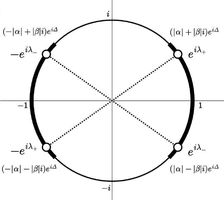
(a)

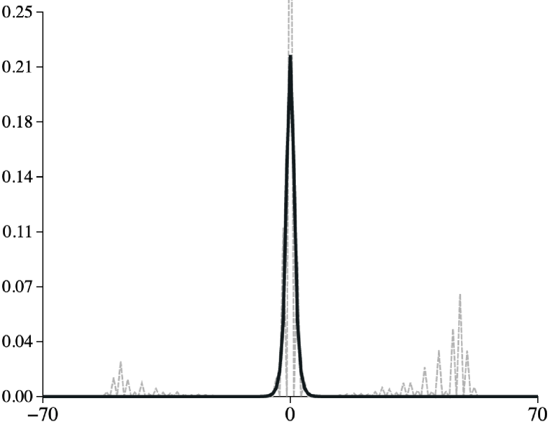
(b)

Figure 1: Example of Model 1 with parameters $\Delta_{o}=\Delta=0,\alpha=\alpha_{o}=\beta=\frac{1}{\sqrt{2}},\beta_{o}=\frac{i}{\sqrt{2}},\psi_{1}=\frac{1}{\sqrt{2}},\psi_{2}=\frac{1}{\sqrt{2}}$, which is strongly trapped. (a) illustrates the eigenvalues, and the bold lines indicate the range of the existence of eigenvalues when $|\beta|$ is fixed. (b) shows the probability distribution at time $t=70$ (dotted line) and the time-averaged limit distribution (bold black line), where the horizontal axis indicates position $x$.

$\bullet\$Example : Figure 1 shows the example.

Model 2.

We assume $(\alpha_{p},\beta_{p},\Delta_{p})=(\alpha_{m},\beta_{m},\Delta_{m})=(\alpha,\beta,\Delta)$ and $\beta_{o}=\beta$.
$\bullet\$Eigenvalues :
$\sigma_{p}(U)\neq\emptyset$ if and only if the following Condition 2a or Condition 2b holds:

1. Condition 2a : $\gamma_{+}=|\beta|\cos(\Delta-\Delta_{o})+|\alpha|\sin(\Delta-\Delta_{o})<|\beta|$,

2. Condition 2b : $\gamma_{-}=|\beta|\cos(\Delta-\Delta_{o})-|\alpha|\sin(\Delta-\Delta_{o})<|\beta|$.

The set of eigenvalues $\sigma_{p}(U)$ is given as follows:

$$\sigma_{p}(U)=\begin{cases}\{\pm e^{i\lambda_{+}}\},&\,\text{2a holds and 2b does not,}\\ \{\pm e^{i\lambda_{-}}\},&\,\text{2b holds and 2a does not,}\\ \{\pm e^{i\lambda_{+}},\pm e^{i\lambda_{-}}\},&\,\text{Both conditions hold,}\end{cases}$$

where

$$e^{i\lambda_{\pm}}=\dfrac{e^{i\Delta}-|\beta|(|\beta|\pm i|\alpha|)e^{i\Delta_{o}}}{|e^{i\Delta}-|\beta|(|\beta|\pm i|\alpha|)e^{i\Delta_{o}}|}.$$

$\bullet\$Eigenvectors :
The associated eigenvectors of $\pm e^{i\lambda_{s}},(s\in\{+,-\})$ are as below:

$$\Psi_{\pm}^{s}(x)=\pm N\begin{cases}\dfrac{-si|\alpha||\beta|}{\alpha_{o}\overline{\alpha}\overline{\beta}}\begin{bmatrix}\overline{\alpha}|\beta|\left(|\beta|-(|\beta|-is|\alpha|)e^{i(\Delta-\Delta_{o})}\right)\\ \overline{\beta}\left(1-2|\beta|\gamma_{s}+|\beta|^{2}\right)\end{bmatrix}\left(\zeta^{<}\right)^{x},&x\geq 1,\\[15.0pt] \dfrac{-|\beta|\left(|\beta|-(|\beta|-is|\alpha|)e^{i(\Delta-\Delta_{o})}\right)}{\alpha_{o}\overline{\beta}}\begin{bmatrix}si|\alpha||\beta|\\ \alpha_{o}\overline{\beta}\end{bmatrix},&x=0,\\[15.0pt] \dfrac{1}{\alpha}\begin{bmatrix}\beta\left(1-2|\beta|\gamma_{s}+|\beta|^{2}\right)\\ -\alpha|\beta|\left(|\beta|-(|\beta|-is|\alpha|)e^{i(\Delta-\Delta_{o})}\right)\end{bmatrix}\left(\zeta^{>}\right)^{x},&x\leq-1,\end{cases}$$

where

$$\zeta^{<}=\pm\dfrac{\overline{\alpha}}{\sqrt{1-2|\beta|\gamma_{s}+|\beta|^{2}}},\ \ \zeta^{>}=\pm\dfrac{\sqrt{1-2|\beta|\gamma_{s}+|\beta|^{2}}}{\alpha},$$

and $N$ is the normalized constant given as below:

$$N=\dfrac{\sqrt{(|\beta|-\gamma_{s})}}{\sqrt{2|\beta|}\left(1-2|\beta|\gamma_{s}+|\beta|^{2}\right)}.$$

$\bullet\$Time-averaged limit distribution :

$$\overline{\nu}_{\infty}(x)=I_{+}\overline{\nu}^{+}_{\infty}(x)+I_{-}\overline{\nu}^{-}_{\infty}(x),$$

where

$$\ I_{+}=\begin{cases}1,&\gamma_{+}<|\beta|,\\ 0,&\gamma_{+}\geq|\beta|,\end{cases}\qquad I_{-}=\begin{cases}1,&\gamma_{-}<|\beta|,\\ 0,&\gamma_{-}\geq|\beta|,\end{cases}$$

and

$$\overline{\nu}_{\infty}^{\pm}(x)=C(\psi_{1},\psi_{2})\begin{cases}\dfrac{1-|\beta|\gamma_{\pm}}{|\alpha|^{2}}\left(\dfrac{|\alpha|^{2}}{1-2|\beta|\gamma_{\pm}+|\beta|^{2}}\right)^{x},&x\geq 1,\\ 1,&x=0,\\ \dfrac{1-|\beta|\gamma_{\pm}}{|\alpha|^{2}}\left(\dfrac{|\alpha|^{2}}{1-2|\beta|\gamma_{\pm}+|\beta|^{2}}\right)^{-x},&x\leq-1,\end{cases}$$

where

$$C(\psi_{1},\psi_{2})=\dfrac{|\beta|(|\beta|-\gamma_{\pm})^{2}\left(|\alpha||\beta|\pm 2\Im\left(\alpha_{0}\overline{\beta}\psi_{1}\overline{\psi_{2}}\right)\right)}{|\alpha|\left(1-2|\beta|\gamma_{\pm}+|\beta|^{2}\right)^{2}}.$$

$\bullet\$Strong trapping : This model is strongly trapped only in the case both Condition 2a and Condition 2b hold. In the other cases, the model is not strongly trapped.

Proof.

If only one of the conditions holds, then $\Psi_{+}^{s}(0)$ and $\Psi_{-}^{s}(0)$ are obviously linear dependent, and Theorem 2.8 shows the QW is not strongly tapped. On the other hand, if both conditions hold, then $\Psi_{+}^{+}(0)$ and $\Psi_{+}^{-}(0)$ are linear independent, so this QW is strongly trapped. ∎

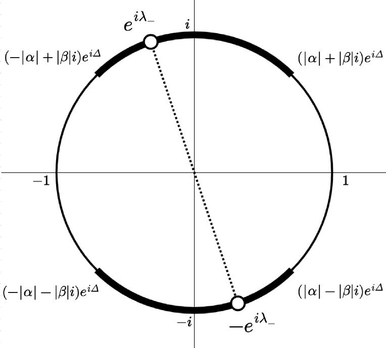
(a)

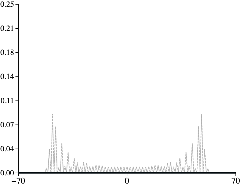
(b)

Figure 2: Example of Model 2 with parameters $\Delta_{o}=0,\Delta=\frac{\pi}{2},\ \alpha=\beta=\alpha_{o}=\beta_{o}=\frac{1}{\sqrt{2}},\psi_{1}=\frac{1}{\sqrt{2}},\psi_{2}=\frac{-i}{\sqrt{2}}$, which is not strongly trapped. (a) illustrates the eigenvalues, and the bold lines indicate the range of the existence of eigenvalues when $|\beta|$ is fixed. (b) shows the probability distribution at time $t=70$ (dotted line), where the horizontal axis indicates position $x$. In this case, the time-averaged distribution becomes 0 for any $x\in\mathbb{Z}$ with this specific initial state.

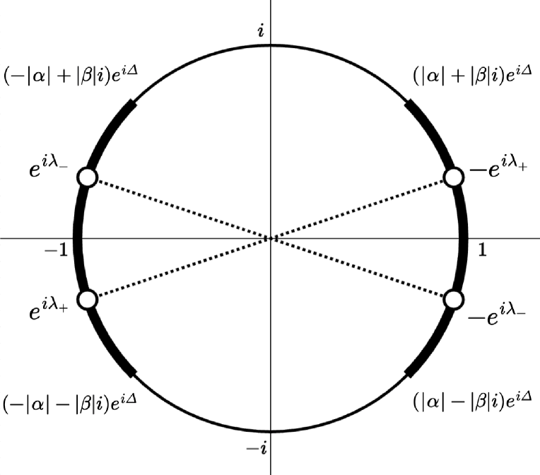
(a)

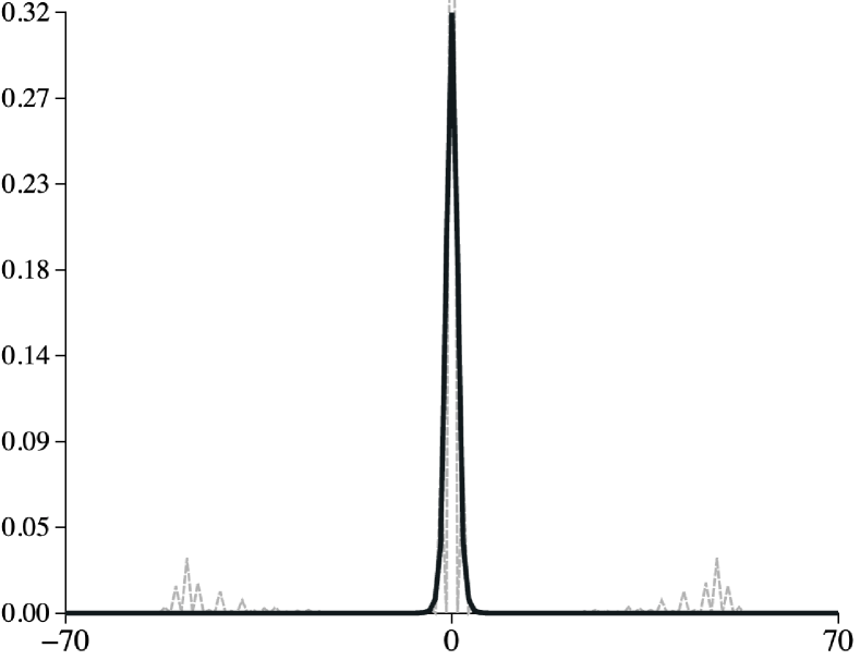
(b)

Figure 3: Example of Model 2 with parameters $\Delta_{o}=0,\Delta=\pi,\ \alpha=\beta=\alpha_{o}=\beta_{o}=\frac{1}{\sqrt{2}},\psi_{1}=\frac{1}{\sqrt{2}},\psi_{2}=\frac{-i}{\sqrt{2}}$ , which is strongly trapped. (a) illustrates the eigenvalues, and the bold lines indicate the range of the existence of eigenvalues when $|\beta|$ is fixed. (b) shows the probability distribution at time $t=70$ (dotted line) and the time-averaged limit distribution (bold black line), where the horizontal axis indicates position $x$.

$\bullet\$Example : Figure 2 shows the example of not strongly trapped case, and Figure 3 shows strongly trapped case.

Model 3.

We assume $(\alpha_{o},\beta_{o},\Delta_{o})=(\alpha_{p},\beta_{p},\Delta_{p})$ and $\arg\beta_{p}=\arg\beta_{m}$.
$\bullet\$Eigenvalues :
$\sigma_{p}(U)\neq\emptyset$ if and only if $\cos\left(\Delta_{m}-\Delta_{p}\right)<\left\lvert\beta_{m}\right\rvert\left\lvert\beta_{p}\right\rvert-\left\lvert\alpha_{m}\right\rvert\left\lvert\alpha_{p}\right\rvert$ holds. If this condition holds, the set of eigenvalues is $\sigma_{p}(U)=\{\pm e^{i\lambda}\}$, where

$$e^{i\lambda}=\dfrac{\left\lvert\beta_{p}\right\rvert e^{i\Delta_{m}}-\left\lvert\beta_{m}\right\rvert e^{i\Delta_{p}}}{||\beta_{p}|e^{i\Delta_{m}}-|\beta_{m}|e^{i\Delta_{p}}|}.$$

$\bullet\$Eigenvectors :
The associated eigenvectors of $\pm e^{i\lambda}$ are given as follows:

$$\Psi_{\pm}(x)=\pm N\begin{cases}\dfrac{1}{\alpha_{p}}\begin{bmatrix}\beta_{m}\left(P+|\beta_{p}|\sqrt{K}\right)\\ -\alpha_{p}|\beta_{m}|\left(i\sin(\Delta_{p}-\Delta_{m})+\sqrt{K}\right)\end{bmatrix}\left(\zeta_{p}^{<}\right)^{x},&x\geq 0,\\[15.0pt] \dfrac{1}{\alpha_{m}}\begin{bmatrix}\beta_{m}(M+|\beta_{m}|\sqrt{K})\\ -\alpha_{m}|\beta_{m}|\left(i\sin(\Delta_{p}-\Delta_{m})+\sqrt{K}\right)\end{bmatrix}\left(\zeta_{m}^{>}\right)^{x},&x\leq-1,\end{cases}$$

where

$$\zeta_{p}^{<}=\pm\dfrac{\left(P+|\beta_{p}|\sqrt{K}\right)}{\alpha_{p}\sqrt{|\beta_{p}|M-|\beta_{m}|P}},\ \zeta_{m}^{>}=\pm\dfrac{\left(M+|\beta_{m}|\sqrt{K}\right)}{\alpha_{m}\sqrt{|\beta_{p}|M-|\beta_{m}|P}},$$

and $N$ is the normalized constant given as below:

$$N=\dfrac{\sqrt{|\beta_{m}|\sqrt{K}}}{\sqrt{|\beta_{m}|}(|\beta_{p}|M-|\beta_{m}|P)},$$

Here,

$$P=|\beta_{p}|\cos(\Delta_{p}-\Delta_{m})-|\beta_{m}|,\quad M=|\beta_{p}|-|\beta_{m}|\cos(\Delta_{p}-\Delta_{m}),$$

$$K=(\cos(\Delta_{p}-\Delta_{m})-|\beta_{p}||\beta_{m}|-|\alpha_{p}||\alpha_{m}|)(\cos(\Delta_{p}-\Delta_{m})-|\beta_{p}||\beta_{m}|+|\alpha_{p}||\alpha_{m}|).$$

$\bullet\$Time-averaged limit distribution :

$$\overline{\nu}_{\infty}(x)=C(\psi_{1},\psi_{2})\begin{cases}\dfrac{P(P+|\beta_{p}|\sqrt{K})}{|\alpha_{p}|^{2}}\left\lvert\zeta_{p}^{<}\right\rvert^{2x},&x\geq 0,\\ \dfrac{M\left(M+|\beta_{m}|\sqrt{K}\right)}{|\alpha_{m}|^{2}}\left\lvert\zeta_{m}^{>}\right\rvert^{2x},&x\leq-1,\end{cases}$$

where

$$C(\psi_{1},\psi_{2})=\dfrac{4|\beta_{m}||\beta_{p}|^{2}K\left(|\alpha_{p}|^{2}|\beta_{m}|(|\beta_{p}|M-|\beta_{m}|P)-2\left(P+|\beta_{p}|\sqrt{K}\right)c(\psi_{1},\psi_{2})\right)}{|\alpha_{p}|^{2}(|\beta_{p}|M-|\beta_{m}|P)^{4}},$$

and

$$c(\psi_{1},\psi_{2})=\left(\Re\left(\alpha_{p}\overline{\beta_{m}}\psi_{1}\overline{\psi_{2}}\right)-|\beta_{m}||\beta_{p}||\psi_{1}|^{2}\right)\sqrt{K}-\sin(\Delta_{p}-\Delta_{m})\Im\left(\alpha_{p}\overline{\beta_{m}}\psi_{1}\overline{\psi_{2}}\right).$$

$\bullet\$Strong trapping : This model is not strongly trapped.

Proof.

$\Psi_{+}(0)$ and $\Psi_{-}(0)$ are obviously linear dependent, so Theorem 2.8 shows the claim. ∎

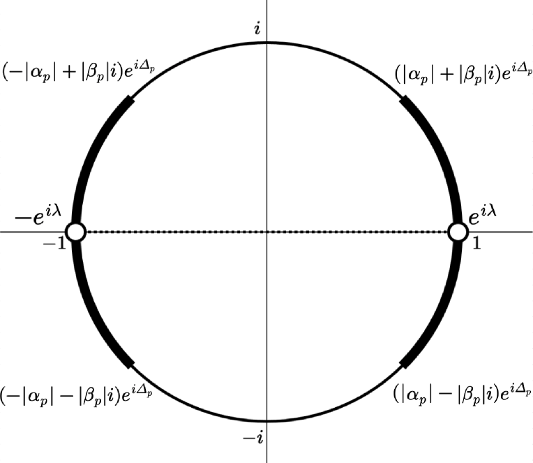
(a)

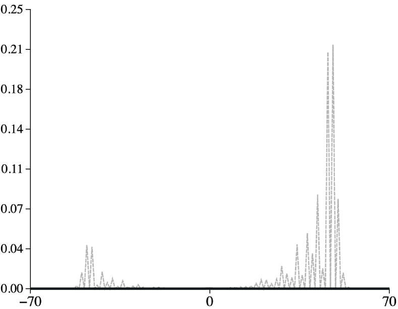
(b)

Figure 4: Example of Model 3 with parameters $\Delta_{p}=\pi,\Delta_{m}=0,\ \alpha_{p}=\beta_{p}=\alpha_{m}=\beta_{m}=\frac{1}{\sqrt{2}},\psi_{1}=\frac{1}{2}\sqrt{2+\sqrt{2}},\psi_{2}=-\frac{1}{2}\sqrt{2-\sqrt{2}}$, which is not strongly trapped. (a) illustrates the eigenvalues, and the bold lines indicate the range of the existence of eigenvalues when $|\beta_{p}|$ is fixed. (b) shows the probability distribution at time $t=70$ (dotted line), where the horizontal axis indicates position $x$. In this case, the time-averaged distribution becomes 0 for any $x\in\mathbb{Z}$ with this specific initial state.

$\bullet\$Example : Figure 4 shows the example.

Model 4.

We assume $(\alpha_{o},\beta_{o},\Delta_{o})=(\alpha_{p},\beta_{p},\Delta_{p})$ and $\Delta_{p}=\Delta_{m}=\Delta$.
$\bullet\$Eigenvalues :
$\sigma_{p}(U)\neq\emptyset$ if and only if $PM>0$ holds, where

$$P=|\beta_{p}|^{2}-\Re\left(\beta_{m}\overline{\beta_{p}}\right),\qquad M=|\beta_{m}|^{2}-\Re\left(\beta_{m}\overline{\beta_{p}}\right).$$

If this condition holds, then the set of eigenvalues is $\sigma_{p}(U)=\{\pm e^{i\lambda}\}$, where

$$e^{i\lambda}=\dfrac{e^{i\Delta}\left(\sqrt{K}+i\Im\left(\beta_{m}\overline{\beta_{p}}\right)\right)}{\left\lvert\beta_{p}-\beta_{m}\right\rvert},$$

$$K=\left(\Re\left(\beta_{m}\overline{\beta_{p}}\right)+|\alpha_{p}||\alpha_{m}|-1\right)\left(\Re\left(\beta_{m}\overline{\beta_{p}}\right)-|\alpha_{p}||\alpha_{m}|-1\right).$$

$\bullet\$Eigenvectors :
The associated eigenvectors of $\pm e^{i\lambda}$ are given as follows:

$$\ \Psi_{\pm}(x)=\pm N\begin{cases}\dfrac{1}{\alpha_{p}}\begin{bmatrix}-P+\sqrt{K}\\ \alpha_{p}\left(\overline{\beta_{p}}-\overline{\beta_{m}}\right)\end{bmatrix}\left(\zeta_{p}^{<}\right)^{x},&x\geq 0,\\[15.0pt] \dfrac{1}{\alpha_{m}}\begin{bmatrix}M+\sqrt{K}\\ \alpha_{m}\left(\overline{\beta_{p}}-\overline{\beta_{m}}\right)\end{bmatrix}\left(\zeta_{m}^{>}\right)^{x},&x\leq-1,\end{cases}$$

where

$$\zeta_{p}^{<}=\pm\dfrac{-P+\sqrt{P+M-\mathfrak{I}^{2}\left(\beta_{m}\overline{\beta_{p}}\right)}}{\alpha_{p}\sqrt{P+M}},\ \ \zeta_{m}^{>}=\pm\dfrac{M+\sqrt{P+M-\mathfrak{I}^{2}\left(\beta_{m}\overline{\beta_{p}}\right)}}{\alpha_{m}\sqrt{P+M}},$$

and $N$ is the normalized constant given as below:

$$N=\dfrac{\beta_{m}}{|\beta_{m}|(P+M)}\sqrt{\dfrac{PM}{\sqrt{K-\mathfrak{I}^{2}\left(\beta_{m}\overline{\beta_{p}}\right))}}}.$$

$\bullet\$Time-averaged limit distribution :

$$\overline{\nu}_{\infty}(x)=C(\psi_{1},\psi_{2})\begin{cases}\dfrac{\left(\sqrt{K}-P\right)}{|\alpha_{p}|^{2}}\ \left\lvert\zeta_{p}^{<}\right\rvert^{2x},&x\geq 0,\\ \dfrac{\left(M+\sqrt{K}\right)}{|\alpha_{m}|^{2}}\left\lvert\zeta_{m}^{>}\right\rvert^{2x},&x\leq-1,\end{cases}$$

where

$$C(\psi_{1},\psi_{2})=\dfrac{4P^{2}M^{2}\left((P+M)|\alpha_{p}|^{2}+2\left(\Re\left(\alpha_{p}\left(\overline{\beta_{p}}-\overline{\beta_{m}}\right)\psi_{1}\overline{\psi_{2}}\right)-P|\psi_{1}|^{2}\right)\left(\sqrt{K}-P\right)\right)}{(P+M)^{4}|\alpha_{p}|^{2}\sqrt{K}}.$$

$\bullet\$Strong trapping : This model is not strongly trapped.

Proof.

$\Psi_{+}(0)$ and $\Psi_{-}(0)$ are obviously linear dependent, so Theorem 2.8 shows the claim. ∎

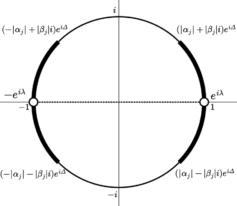
(a)

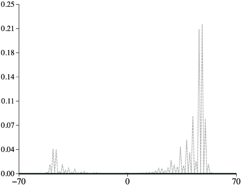
(b)

Figure 5: Example of Model 4 with parameters $\Delta=0,\ \alpha_{p}=\alpha_{m}=\beta_{m}=\frac{1}{\sqrt{2}},\beta_{p}=-\frac{1}{\sqrt{2}},\ \phi_{1}=\frac{1}{2}\sqrt{2+\sqrt{2}},\phi_{2}=\frac{1}{2}\sqrt{2-\sqrt{2}}$, which is not strongly trapped. (a) illustrates the eigenvalues, and the bold lines indicate the range of the existence of eigenvalues when $|\beta_{j}|\ (j=p\left(\left\lvert\beta_{p}\right\rvert\leq\left\lvert\beta_{m}\right\rvert\right),=m\left(\left\lvert\beta_{m}\right\rvert<\left\lvert\beta_{p}\right\rvert\right))$ is fixed. (b) shows the probability distribution at time $t=70$ (dotted line), where the horizontal axis indicates position $x$. In this case, the time-averaged distribution becomes 0 for any $x\in\mathbb{Z}$ with this specific initial state.

$\bullet\$Example : Figure 5 shows the example.

Model 5.

We assume $\beta_{o}=0$, $\ |\beta_{p}|=|\beta_{m}|=|\beta|$ and $\Delta_{p}=\Delta_{m}=\Delta$.
$\bullet\$Eigenvalues :
Let $\gamma=\Delta_{o}+(\arg\beta_{p}-\arg\beta_{m})/2$. Then $\sigma_{p}(U)\neq\emptyset$ if and only if the following Condition 5a or Condition 5b holds:

1. Condition 5a : $\sin(\Delta-\gamma)\in(-|\beta|,1]$,

2. Condition 5b : $\sin(\Delta-\gamma)\in[-1,|\beta|)$.

The set of eigenvalues $\sigma_{p}(U)$ is given as follows:

$$\sigma_{p}(U)=\begin{cases}\{\pm e^{i\lambda_{+}}\},&\quad\text{Condition 5a holds and 5b does not,}\\ \{\pm e^{i\lambda_{-}}\},&\quad\text{Condition 5b holds and 5a does not,}\\ \{\pm e^{i\lambda_{+}},\ \pm e^{i\lambda_{-}}\},&\quad\text{Both conditions hold,}\end{cases}$$

where

$$e^{i\lambda_{\pm}}=\dfrac{e^{i\Delta}\pm i|\beta|e^{i\gamma}}{|e^{i\Delta}\pm i|\beta|e^{i\gamma}|}.$$

$\bullet\$Eigenvectors :
The associated eigenvectors of $\pm e^{i\lambda_{s}},(s\in\{+,-\})$ are given as follows:

$$\Psi_{\pm}^{s}(x)=\pm N\begin{cases}\dfrac{1}{\alpha_{o}\overline{\alpha_{p}}}\begin{bmatrix}\overline{\alpha_{p}}\beta_{m}e^{i(\Delta-\Delta_{0})}\left(1+si|\beta|e^{-i(\Delta-\gamma)}\right)\\ si|\beta|A_{s}e^{i(\Delta_{o}-\gamma)}\end{bmatrix}\left(\zeta_{p}^{<}\right)^{x},&x\geq 1,\\[15.0pt] \dfrac{1}{\alpha_{o}}\begin{bmatrix}\beta_{m}e^{i(\Delta-\Delta_{o})}\left(1+si|\beta|e^{-i(\Delta-\gamma)}\right)\\ -\alpha_{o}|\beta|\left(|\beta|-sie^{i(\Delta-\gamma)}\right)\end{bmatrix},&x=0,\\[15.0pt] \dfrac{1}{\alpha_{m}}\begin{bmatrix}\beta_{m}A_{s}\\ -\alpha_{m}|\beta|\left(|\beta|-sie^{i(\Delta-\gamma)}\right)\end{bmatrix}\left(\zeta_{m}^{>}\right)^{x},&x\leq-1,\end{cases}$$

where

$$A_{\pm}=1\pm 2|\beta|\sin(\Delta-\gamma)+|\beta|^{2},\ \ \ \zeta_{p}^{<}=\pm\dfrac{\overline{\alpha_{p}}}{\sqrt{A_{s}}},\ \ \zeta_{m}^{>}=\pm\dfrac{\sqrt{A_{s}}}{\alpha_{m}},$$

and $N$ is the normalized constant given as below:

$$N=\sqrt{\dfrac{|\beta|+s\sin(\Delta-\gamma)}{2|\beta|A_{s}^{2}}}.$$

$\bullet\$Time-averaged limit distribution :

$$\overline{\nu}_{\infty}(x)=I_{+}\overline{\nu}^{+}_{\infty}(x)+I_{-}\nu^{-}_{\infty}(x),$$

where

$$\ I_{+}=\begin{cases}1,&\sin(\Delta-\gamma)\in(-|\beta|,1],\\ 0,&\sin(\Delta-\gamma)\in[-1,-|\beta|],\end{cases}\ \ \ \ I_{-}=\begin{cases}1,&\sin(\Delta-\gamma)\in[-1,|\beta|),\\ 0,&\sin(\Delta-\gamma)\in[|\beta|,1].\end{cases}$$

and

$$\overline{\nu}_{\infty}^{\pm}(x)=C(\psi_{1},\psi_{2})\begin{cases}\dfrac{1\pm|\beta|\sin(\Delta-\gamma)}{|\alpha|^{2}}\left(\dfrac{|\alpha|^{2}}{A_{\pm}}\right)^{x},&x\geq 1,\\ 1,&x=0,\\ \dfrac{1\pm|\beta|\sin(\Delta-\gamma)}{|\alpha|^{2}}\left(\dfrac{|\alpha|^{2}}{A_{\pm}}\right)^{-x},&x\leq-1,\end{cases}$$

where

$$C(\psi_{1},\psi_{2})=\dfrac{(|\beta|\pm\sin(\Delta-\gamma))^{2}\left(|\beta|^{2}\mp 2|\beta|\Im\left(e^{i(\Delta_{o}-\gamma)}\alpha_{o}\overline{\beta_{m}}\psi_{1}\overline{\psi_{2}}\right)\right)}{A_{\pm}^{2}}.$$

$\bullet\$Strong trapping :
This model is strongly trapped only in the case both Condition 5a and Condition 5b hold. In the other cases, the QWs is not strongly trapped.

Proof.

If only one of the conditions holds, then $\Psi_{+}^{s}(0)$ and $\Psi_{-}^{s}(0)$ are obviously linear dependent, and Theorem 2.8 shows the QW is not strongly tapped. On the other hand, if both conditions hold, then $\Psi_{+}^{+}(0)$ and $\Psi_{+}^{-}(0)$ are linear independent, so this QW is strongly trapped. ∎

$\bullet\$Example : Figure 6 shows the example of not strongly trapped case, and Figure 7 show strongly trapped case.

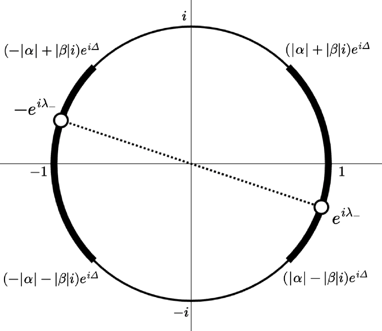
(a)

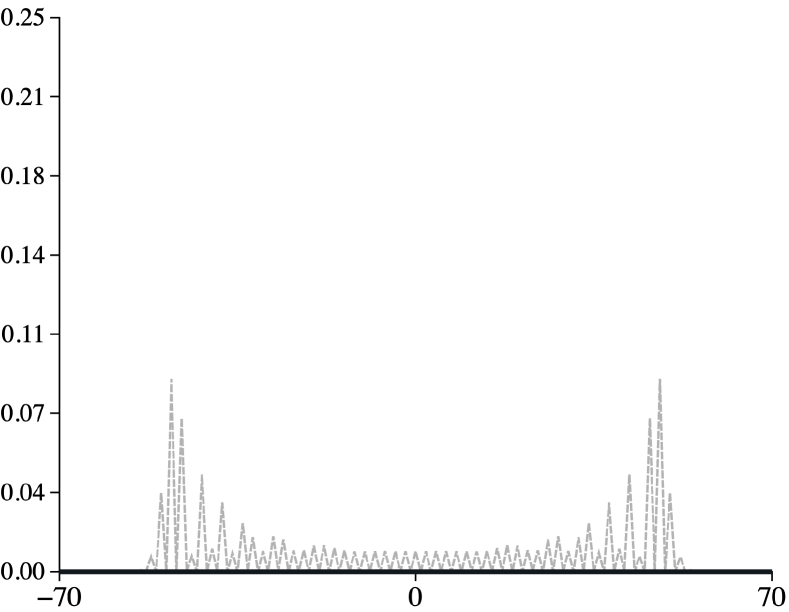
(b)

Figure 6: Example of Model 5 with parameters $\Delta=\Delta_{o}=0,\alpha_{o}=1,\ \alpha_{p}=\alpha_{m}=\beta_{m}=\frac{1}{\sqrt{2}},\beta_{p}=\frac{i}{\sqrt{2}},\psi_{1}=\frac{1}{\sqrt{2}},\psi_{2}=\frac{1}{\sqrt{2}}e^{i\frac{\pi}{4}}$, which is not strongly trapped. (a) illustrates the eigenvalues, and the bold lines indicate the range of the existence of eigenvalues when $|\beta|$ is fixed. (b) shows the probability distribution at time $t=70$ (dotted line), where the horizontal axis indicates position $x$. In this case, the time-averaged distribution becomes 0 for any $x\in\mathbb{Z}$ with this specific initial state.

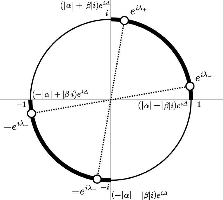
(a)

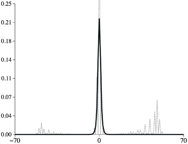
(b)

Figure 7: Example of Model 5 with parameters $\Delta=\frac{\pi}{4},\Delta_{o}=0,\alpha_{o}=1,\ \alpha_{p}=\alpha_{m}=\beta_{m}=\frac{1}{\sqrt{2}},\beta_{p}=\frac{i}{\sqrt{2}},\psi_{1}=\frac{1}{\sqrt{2}},\psi_{2}=\frac{1}{\sqrt{2}}$ , which is strongly trapped. (a) illustrates the eigenvalues, and the bold lines indicate the range of the existence of eigenvalues when $|\beta|$ is fixed. (b) shows probability distribution at time $t=70$ (dotted line) and the time-averaged limit distribution (bold black line), where the horizontal axis indicates position $x$.

4 Summary

This paper is a continuation of our previous study [12], which concentrates on the eigenvalues of the time evolution operator for two-phase QWs with one defect. In this paper, we focused on the quantitative study of localization and strong trapping property by deriving time-averaged limit distributions on space-inhomogeneous QWs on the integer lattice $\mathbb{Z}$. In Section 2, we introduced the definitions of our model and gave the method to formulate eigenvectors of time evolution operator. Moreover, we showed some results to characterize eigenvalues not only for two-phase QWs with one defect but also for the more general space-inhomogeneous model. The necessary and sufficient condition for the eigenvectors was shown in Theorem 2.3. We also defined the strong trapping with the time-averaged limit distribution, which can be calculated with eigenvectors. In Section 3, we derived eigenvectors and time-averaged limit distributions for five models whose eigenvalues were derived in the main theorems in the authors’ previous study [12]. Models 1 and 2 are one-defect QWs, models 3 and 4 are two-phase QWs, and model 5 are two-phase QWs with one defect. Furthermore, the class of strong trapping was also revealed for these models.

Appendix

In the appendix, we give an abstract form of time-averaged limit distribution of two-phase quantum walks with one defect. As denoted in Section 2.2, we remark that the time-averaged limit distribution with initial state $\Psi_{0}\in\mathcal{H}$ is written by the following.

$$\overline{\nu}_{\infty}(x)=\sum_{e^{i\lambda}\in\sigma_{p}(U)}\left|\left\langle\Psi^{\lambda}\,,\,\Psi_{0}\right\rangle\right|^{2}\ \|\Psi^{\lambda}(x)\|_{\mathbb{C}^{2}}^{2},$$

where $\Psi^{\lambda}\in\ker(U-e^{i\lambda})$. For eigenvalue $e^{i\lambda}$, we put

$$M=\frac{\alpha_{m}\zeta_{m}^{>}-e^{i(\lambda-\Delta_{m})}}{\beta}e^{-i(\lambda-\Delta_{o})}$$

and normalized constant

$$N=\left(\frac{(1-|\beta_{o}|^{2})(1-|\zeta_{p}^{<}|^{2})+(1+|\beta_{o}|^{2})(1-|\zeta_{m}^{<}|^{2})}{\left(1-|\zeta_{p}^{<}|^{2}\right)\left(1-|\zeta_{m}^{<}|^{2}\right)}+\frac{2\Re(\beta_{o}M)}{1-|\zeta_{p}^{<}|^{2}}\right)^{-1}.$$

Then, associated eigenvector is

$$\Psi^{\lambda}(x)=\sqrt{\dfrac{N}{2}}\begin{cases}\begin{bmatrix}e^{i(\lambda-\Delta_{o})}(1+\beta_{o}M)\\[5.0pt] -(\overline{\beta_{o}}+M)(\zeta_{p}^{<})^{-1}\end{bmatrix}(\zeta_{p}^{<})^{x},\quad&x\geq 1,\\[16.0pt] \begin{bmatrix}e^{i(\lambda-\Delta_{o})}(1+\beta_{o}M)\\[5.0pt] -e^{i(\lambda-\Delta_{o})}\alpha_{o}M\end{bmatrix},\quad&x=0,\\[16.0pt] \begin{bmatrix}\alpha_{o}\zeta_{m}^{>}\\ -e^{i(\lambda-\Delta_{o})}\alpha_{o}M\end{bmatrix}(\zeta_{m}^{>})^{x},\quad&x\leq-1.\end{cases}$$

The key parts of the time-averaged limit distribution are

$$\|\Psi^{\lambda}(x)\|^{2}_{\mathbb{C}^{2}}=N^{2}\begin{cases}\left(\dfrac{1+|\beta_{o}|^{2}}{2}+\Re(\beta_{o}M)\right)\left(1+\left|\zeta_{p}^{>}\right|^{2}\right)\left|\zeta_{p}^{>}\right|^{2x},\quad&x\geq 1,\\[5.0pt] \left(1-\Re(\beta_{o}M)\right),\quad&x=0,\\[5.0pt] \left(\dfrac{1-|\beta_{o}|^{2}}{2}\right)\left(1+\left|\zeta_{m}^{>}\right|^{2}\right)\left|\zeta_{m}^{>}\right|^{2x},\quad&x\leq-1,\end{cases}$$

and

$$\left|\left\langle\Psi^{\lambda}\,,\,\Psi_{0}\right\rangle\right|^{2}=\frac{N^{2}}{2}{\bigg{[}}1+\left(1+2\Re(\beta_{o}M)\right)|\psi_{1}|^{2}-2\Re\left((M+\overline{\beta_{o}})\alpha_{o}\overline{\psi_{1}}\psi_{2}\right){\bigg{]}},$$

where $\Psi_{0}(x)=\begin{bmatrix}\psi_{1}&\psi_{2}\end{bmatrix}^{t}$ with $|\psi_{1}|^{2}+|\psi_{2}|^{2}=1$ if $x=0$, and $=\begin{bmatrix}0&0\end{bmatrix}^{t}$ if $x\neq 0$. Here, $t$ means the transpose operator.

References

- [1] Andris Ambainis et al. “One-dimensional quantum walks” In Proceedings of the thirty-third annual ACM symposium on Theory of computing, STOC ’01 Hersonissos, Greece: Association for Computing Machinery, 2001, pp. 37–49
- [2] M J Cantero, F A Grünbaum, L Moral and L Velázquez “The CGMV method for quantum walks” In Quantum Inf. Process. 11.5 Springer ScienceBusiness Media LLC, 2012, pp. 1149–1192
- [3] Norio Konno “A new type of limit theorems for the one-dimensional quantum random walk” In J. Math. Soc. Japan 57.4, 2005, pp. 1179–1195
- [4] B Kollár, T Kiss and I Jex “Strongly trapped two-dimensional quantum walks” In Phys. Rev. A 91.2 American Physical Society, 2015, pp. 022308
- [5] B Kollár et al. “Complete classification of trapping coins for quantum walks on the two-dimensional square lattice” In Phys. Rev. A 102.1, 2020
- [6] Andris Ambainis, Julia Kempe and Alexander Rivosh “Coins make quantum walks faster” In Proceedings of the sixteenth annual ACM-SIAM symposium on Discrete algorithms, SODA ’05 Vancouver, British Columbia: Society for IndustrialApplied Mathematics, 2005, pp. 1099–1108
- [7] Andrew M Childs and Jeffrey Goldstone “Spatial search by quantum walk” In Phys. Rev. A 70.2 American Physical Society, 2004, pp. 022314
- [8] Neil Shenvi, Julia Kempe and K Birgitta Whaley “Quantum random-walk search algorithm” In Phys. Rev. A 67.5 American Physical Society, 2003, pp. 052307
- [9] Takuya Kitagawa, Mark S Rudner, Erez Berg and Eugene Demler “Exploring topological phases with quantum walks” In Phys. Rev. A 82.3 American Physical Society, 2010, pp. 033429
- [10] Takako Endo, Norio Konno and Hideaki Obuse “Relation between two-phase quantum walks and the topological invariant” In Yokohama Math. J. 64, 2020, pp. 1–59 arXiv:1511.04230
- [11] Etsuo Segawa and Akito Suzuki “Generator of an abstract quantum walk” In Quantum Stud.: Math. Found. 3.1 Springer ScienceBusiness Media LLC, 2016, pp. 11–30
- [12] Chusei Kiumi and Kei Saito “Eigenvalues of two-phase quantum walks with one defect in one dimension” In Quantum Inf. Process. 20.5 Springer ScienceBusiness Media LLC, 2021
- [13] Shimpei Endo, Takako Endo, Takashi Komatsu and Norio Konno “Eigenvalues of Two-State Quantum Walks Induced by the Hadamard Walk” In Entropy 22.1, 2020
- [14] Takako Endo, Norio Konno, Etsuo Segawa and Masato Takei “A one-dimensional Hadamard walk with one defect” In Yokohama Math. J. 60, 2014, pp. 49–90
- [15] Shimpei Endo et al. “Limit theorems of a two-phase quantum walk with one defect” In Quantum Inf. Comput. 15.15&16 Rinton Press, 2015, pp. 1373–1396
- [16] Antoni Wójcik et al. “Trapping a particle of a quantum walk on the line” In Phys. Rev. A 85.1 American Physical Society, 2012, pp. 012329
- [17] B Danacı, G Karpat, İ Yalçınkaya and A L Subaşı “Non-Markovianity and bound states in quantum walks with a phase impurity” In J. Phys. A: Math. Theor. 52.22 IOP Publishing, 2019, pp. 225302
- [18] Hikari Kawai, Takashi Komatsu and Norio Konno “Stationary measure for two-state space-inhomogeneous quantum walk in one dimension” In Yokohama Math. J. 64, 2018, pp. 111–130
- [19] Hikar Kawai, Takashi Komatsu and Noriko Konno “Stationary measures of three-state quantum walks on the one-dimensional lattice” In Yokohama Math. J. 63, 2017, pp. 59–74
- [20] Masaya Maeda et al. “Dispersive estimates for quantum walks on 1D lattice” In J. Math. Soc. Japan Advance Publication Mathematical Society of Japan, 2021, pp. 1–30
- [21] S Richard, A Suzuki and R Tiedra Aldecoa “Quantum walks with an anisotropic coin II: scattering theory” In Lett. Math. Phys. 109.1, 2019, pp. 61–88
- [22] Akito Suzuki “Asymptotic velocity of a position-dependent quantum walk” In Quantum Inf. Process. 15.1 Springer ScienceBusiness Media LLC, 2016, pp. 103–119