Principled information fusion for multi-view multi-agent surveillance systems

Abstract

A key objective of multi-agent surveillance systems is to monitor a much larger region than the limited field-of-view (FoV) of any individual agent by successfully exploiting cooperation among multi-view agents. Whenever either a centralized or a distributed approach is pursued, this goal cannot be achieved unless an appropriately designed fusion strategy is adopted. This paper presents a novel principled information fusion approach for dealing with multi-view multi-agent case, on the basis of Generalized Covariance Intersection (GCI). The proposed method can be used to perform multi-object tracking on both a centralized and a distributed peer-to-peer sensor network. Simulation experiments on realistic multi-object tracking scenarios demonstrate effectiveness of the proposed solution.

I Introduction

The recent breakthrough of wireless sensor network (WSN) technology has made it possible to develop efficient surveillance systems that consist of multiple radio-interconnected, low-cost and low energy consumption devices (agents) with sensing, communication and processing capabilities. In this respect, it has become of paramount importance to redesign multi-object tracking algorithms tailored to the new features of emerging surveillance systems. In particular, a fundamental issue to be suitably addressed is how to consistently fuse information from different agents [1].

As well known, the computational cost of extracting the common information can make the optimal fusion [2] intractable in most practical cases, so that a suboptimal solution with demonstrated tractability has been proposed relying on the generalized covariance intersection (GCI) [3, 4], also called exponential mixture density (EMD) in [5, 6]. From an information-theoretic viewpoint, GCI fusion admits a meaningful interpretation in that the fused density is the left centroid of the local posteriors with Kullback-Leibler divergence (from local to fused density) considered as distance; accordingly, GCI fusion is also called Kullback-Leibler average (KLA) in [1, 7]. It has been mathematically proved that the KLA intrinsically avoids double counting of common information [7]. Implementation of GCI fusion combined with a variety of multi-object trackers including PHD, CPHD, multi-Bernoulli as well as certain labeled random finite set (RFS) filters has been investigated in [1, 8, 9, 10].

Another relevant issue, that has recently received growing attention in the literature, is that, due to the limited sensing ability, individual sensor nodes can typically detect objects within a limited range and/or angle. In a multi-agent surveillance system, agent nodes are deployed in different locations of the surveillance area, thus having partially/non-overlapping fields of view (FoVs). A potential benefit of having a multi-view multi-agent surveillance system is actually to extend the FoV of an individual sensor node to a much larger one, with the ultimate goal to make the latter equal to the union of the FoVs of all individual sensor nodes in the network (called global FoV). To achieve this ultimate goal, information fusion among multiple agents needs to achieve sufficient and valid information gain within the global FoV.

Standard GCI fusion provides unsatisfactory performance for the multi-view case in that it tends to preserve only the objects that are in the intersection of the FoVs of all nodes involved in the fusion (common FoV). In order to overcome this mis-behavior of standard GCI fusion, some improved fusion strategies aiming at certain classes of multi-object densities have been presented in the literature [11, 12, 13, 14, 18, 19, 20, 15, 16, 17] for multi-view multi-object estimation problems. In particular, [11] concerns multi-robot PHD-based distributed map construction with different robot FoVs, and proposes to initialize the local density of each agent to an uninformative (flat) prior over the global FoV. Further, multi-sensor fusion with different FoVs for the LMB filter is addressed in [12], wherein a suitable compensation strategy for the exclusive FoV to be applied before GCI fusion is proposed. The use of a compensation strategy is further investigated in [13] where distributed fusion with a multi-view sensor network using PHD filters is considered. In [14], an intuitive approach which tunes the weights of LMB posteriors automatically according to amount of information is proposed to overcome the drawback of GCI fusion for centralized fusion. A further proposal has been to replace GCI fusion, penalized by its multiplicative nature, with additive mixture density (AMD) fusion [18, 19, 20, 15, 16, 17].

However, the analysis in this paper will show how the mis-behaviour of standard GCI fusion is mainly due to the inconsistency of the local multi-object density outside the FoV, rather than to the multiplicative nature of GCI. For an independently-working agent, multi-object filtering usually truncates the density outside the FoV for the sake of computational feasiblity, leading to a multi-object posterior with nearly null yes-probability outside the individual FoV. This feature of the multi-object posterior has clearly no influence on the performance of independently-working agents, since the region outside the FoV is not of interest. However, our analysis shows that, for multi-agent fusion with partially/non-overlapping FoVs, whenever the local posterior is fused with other agent densities according to the GCI rule, the fused density will have null yes-probability outside the common FoV (which means that no object existence can be declared outside the common FoV). As a direct consequence for object tracking, only tracks within the common FoV can be preserved after fusion, while other tracks are lost. Such null yes-probability indicates a zero information entropy, conveying specific information that objects cannot exist outside the common FoV, which is obviously inconsistent with the fact that each individual sensor cannot receive measurements of objects outside the FoV.

To avoid null yes-probability outside the common FoV, a consistent propagation of the multi-object posterior is of crucial importance. A first possibility is to restrict measurement update to the local FoV, and only apply prediction outside the FoV, which is the natural result of the local filtering by setting to zero the probability of detection outside the FoV for the multi-object likelihood. However, prediction of the multi-object density can induce a significant bias with respect to the true multi-object state, especially when some object moves in the exclusive FoV of a certain sensor for a long time.

Conversely, in the present paper, we provide a rigorous mathematical definition of multi-object uninformative density. Such a density reflects the complete unavailability of multi-object information and, therefore, represents a consistent form for the posterior outside the FoV of each agent.

The contributions of this paper can be summarized as follows.

1. First, we propose a novel principled information fusion rule for a multi-view multi-agent surveillance system, called Bayesian-operation InvaRiance on Difference-sets (BIRD), on the basis of the GCI which can satisfactorily cope with both centralized and distributed fusion.

2. Then, the proposed BIRD fusion is applied to multi-object Poisson processes and, accordingly, a multi-view multi-agent fusion algorithm under the PHD filtering framework is developed.

3. Finally, it is shown how the proposed BIRD PHD fusion for multi-object tracking can be implemented over a peer-to-peer sensor network in a fully distributed manner via a Gaussian mixture (GM) approach.

In addition to the proposed multi-view fusion rule, we also provide two basic mathematical tools that fill some blanks in the FInite Set STatistics (FISST) [21].

1. The marginal and conditional densities with respect to disjoint subspaces of the RFS, which further enable a general and accurate decomposition of RFS densities.

2. An RFS-based multi-object uninformative density, to be used as multi-object prior whenever there is no available prior knowledge. Note that, to the best of the authors’ knowledge, this is the first time that an RFS-based uninformative density is proposed in a rigorous way.

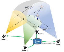
(a)

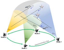
(b)

Figure 1: Examples of multi-view sensor network : (a) centralized network; (b) distributed peer-to-peer network.

II Problem formulation and mathematical tools

II-A Network model

This work considers two types of networks as depicted in Figs. 1 (a) and (b), namely the centralized and distributed peer-to-peer network. Each sensor node (agent) $i\in\mathcal{N}$ has a limited Field-of-View (FoV), denoted by $Fov_{i}$, where $\mathcal{N}=\{1,\cdots,N_{s}\}$ is the set of nodes. Let $\mathbb{X}$ denotes the object state space. Herein each $Fov_{i}$ is defined as a finite subset of $\mathbb{X}$, i.e. $Fov_{i}\in\mathcal{F}(\mathbb{X})$. Specifically, each sensor node $i$ can only receive measurements of kinematic variables (e.g., angles, distances, Doppler shifts, etc.) relative to objects states within $Fov_{i}$. The global FoV of the network, denoted by $Fov_{G}$, is the union of the FoVs of all sensor nodes, i.e. $Fov_{G}=\displaystyle{\cup_{i\in\mathcal{N}}}\,Fov_{i}$. Note that to facilitate easy understanding and plotting, the FoVs shown in figures of the paper are the projections of FoVs on the measurement space.

1) Centralized sensor network: The network consists of heterogenous and geographically dispersed nodes with processing, communication and sensing capabilities, as well as of a fusion center. Each node transmits its local posterior to the fusion center, wherein the fusion of all local posteriors is carried out.

2) Distributed sensor network: The distributed network consists only of heterogenous and geographically dispersed nodes with processing, communication and sensing capabilities. Further features are that: 1) there is no central fusion node; 2) nodes are unaware of the network topology, i.e., the number of nodes and their links. The network is represented by a directed graph $\mathcal{G}=(\mathcal{N},\mathcal{A})$ , where $\mathcal{A}\subseteq\mathcal{N}\times\mathcal{N}$ the set of edges, such that $(i,j)\in\mathcal{A}$ if and only if node $j$ is able to receive data from node $i$. For each node $j\in\mathcal{N}$, $\mathcal{N}_{j}=\{i\in\mathcal{N}:(i,j)\in\mathcal{A}\}$ denotes its set of in-neighbors, i.e., the set of nodes from which node $j$ can receive data. By definition, $(j,j)\in\mathcal{A}$ and, hence, $j\in\mathcal{N}_{j}$ for all $j$. Each sensor node can process local data as well as exchange information with its neighbours.

II-B GCI Fusion

GCI fusion has been first proposed by Mahler [3] to develop multi-object tracking in a multi-agent setting. The name GCI stems from the fact that the fusion is the multi-object counterpart of the analogous fusion rule for (single-object) probability densities [5] which, in turn, is a generalization of covariance intersection originally conceived for fusion of Gaussian probability densities [22].

Suppose that, in each node $i\in\mathcal{N}$ of the network, an RFS density $\pi_{i}$, defined over a suitable state space $\mathbb{X}$ and computed on the basis of local information, is available. GCI fusion amounts to computing the geometric mean, or the exponential mixture of the set of the local multi-object densities, i.e.,

$$\begin{split}\overline{\pi}(X)=\frac{\prod_{i\in\mathcal{N}}[\pi_{i}(X)]^{\omega_{i}}}{\int\prod_{i\in\mathcal{N}}[\pi_{i}(X)]^{\omega_{i}}\delta X}\end{split}$$ (1)

where $\int~{}\cdot~{}\delta X$ denotes set integration [21] and fusion weights $\omega_{i}\geqslant 0$ satisfy $\sum_{i\in\mathcal{N}}\omega_{i}=1$.

In [23, 1] it has been shown that the GCI fusion in (1) essentially minimizes the weighted sum of the Kullback-Leibler divergences (KLDs) with respect to the local densities, i.e.,

$$\overline{\pi}=\arg\min_{\pi}\sum_{i\in\mathcal{N}}\omega_{i}D_{\text{KL}}(\pi||\pi_{i})$$ (2)

where $D_{\text{KL}}(\pi||\pi_{i})$ denotes the KLD of $\pi_{i}$ from $\pi$, i.e.,

$$\begin{split}D_{\text{KL}}(\pi||\pi_{i})\triangleq\int\pi(X)\log{\frac{\pi(X)}{\pi_{i}(X)}}\delta X.\end{split}$$ (3)

In view of (2), GCI fusion is also called Kullback-Leibler average (KLA) [1].

For notational simplicity, let us introduce operators $\oplus$ and $\odot$ as

$$\pi\oplus\pi^{\prime} \triangleq\frac{\pi(X)\,\pi^{\prime}(X)}{\int\pi(X)\,\pi^{\prime}(X)\delta X}$$ (4)

$$\omega\odot\pi \triangleq\frac{\pi(X)^{\omega}}{\int\pi(X)^{\omega}\,\delta X}.$$ (5)

Since $\oplus$ is consistent with the Bayes rule [21], taking $\pi^{\prime}(\cdot)$ as prior density and $\pi(\cdot)$ as likelihood, we call $\oplus$ Bayesian operator. Further, $\odot$ is called exponentation operator.

In terms of the operators $\oplus$ and $\odot$, GCI fusion (1) can be re-expressed as

$$\overline{\pi}=\bigoplus_{i\in\mathcal{N}}\,\left(\omega_{i}\odot\pi_{i}\right).$$ (6)

II-C Multi-object uninformative density

In the Bayes’ theorem, the uninformative prior is typically used when there is no available prior information, thus implying that the posterior turns out to be equal to the normalized likelihood. In an early stage, originally postulated that the uninformative prior should be constant. Later, Jeffreys, using heuristic arguments, suggested that a better uninformative prior is the $1/\sigma$ function [24]. Then, Jaynes provided a more formal derivation of the $1/\sigma$ prior for certain classes of probability functions [25]. However, for the RFS case, to the best of the authors’ knowledge, no proper definition of uninformative prior has been given.

In this paper, we first provide the rigorous notion of multi-object uninformative density, which is a key concept for the subsequent developments.

Definition 1.

Consider a family $\digamma$ of RFS densities over a state space $\mathbb{X}$, then $\pi_{ui}$ is uninformative if

$$\pi\oplus\pi_{ui} =\pi, \forall\pi\in\digamma$$ (7)

$$\omega\odot\pi_{ui} =\pi_{ui}, \forall\omega\in[0,1].$$ (8)

Remark 1.

A multi-object uninformative density is the zero-element of the algebra defined by the Bayesian operator $\odot$ and the exponentiation operator $\oplus$.

According to (7), the Bayesian operation between an arbitrary multi-object density $\pi$ and a multi-object uninformative density $\pi_{ui}$, always provides $\pi$ as a result, and hence this property is called as the Bayesian-operator invariance. Furthermore, according to (6) and Definition 1, it is also easy to see that GCI fusion between an arbitrary multi-object density $\pi$ and an uninformative density $\pi_{ui}$, always provides $\pi$ as a result.

II-D Decomposition of a multi-object density with respect to disjoint sub-spaces

For the subsequent developments, we propose now the marginal and conditional densities with respect to disjoint subspaces of the RFS, which enable a general decomposition of RFS densities.

Proposition 1.

Given the RFS $X$ defined on $\mathbb{X}$ with the multi-object density $\pi(X)$, the marginal density of $X_{W}=X\cap\mathbb{W}$ with $\mathbb{W}\subseteq\mathbb{X}$ is given by

$$\begin{split}\pi_{W}(X)=&[1_{\mathbb{W}}]^{X}\int_{\mathbb{V}}\pi(X\cup X^{\prime})\,\delta X^{\prime}\\ \end{split}$$ (9)

where: $\mathbb{V}$ is the complementary set of $\mathbb{W}$, i.e. $\mathbb{V}=\mathbb{X}\backslash\mathbb{W}$; the indicator function $1_{\mathbb{W}}$ is equal to $1$ if $x\in\mathbb{W}$ and to zero otherwise; and

$$\begin{split}&\int_{\mathbb{V}}\pi(X\cup X^{\prime})\delta X^{\prime}\\ =&\sum_{n^{\prime}=0}^{+\infty}\frac{1}{n^{\prime}!}\int_{\mathbb{V}}\prod_{i=1}^{n^{\prime}}\pi(X\cup\{x^{\prime}_{1},\cdots,x^{\prime}_{n^{\prime}}\})d(x^{\prime}_{1},\cdots,x^{\prime}_{n^{\prime}}).\end{split}$$ (10)

Proof: see Section I of the supplemental materials. ∎

For any $\pi_{W}(X)\neq 0$, the density of $X_{V}=X\cap\mathbb{V}$ conditioned on $X_{W}=X\backslash X_{V}$, denoted by $\pi_{V}(X^{\prime}|X)$ is

$$\pi_{V}(X^{\prime}|X)=\frac{[1_{\mathbb{W}}]^{X}[1_{\mathbb{V}}]^{X^{\prime}}\pi(X^{\prime}\cup X)}{\pi_{W}(X)}.$$ (11)

Remark 2.

To check that $\pi_{V}(X^{\prime}|X)$ is an RFS density on $\mathbb{V}$, we further compute its set integral on $\mathbb{V}$ as

$$\begin{split}&\int_{\mathbb{V}}\frac{[1_{\mathbb{W}}]^{X}[1_{\mathbb{V}}]^{X^{\prime}}\pi(X^{\prime}\cup X)}{\pi_{W}(X)}\delta X^{\prime}\\ =&\frac{[1_{\mathbb{W}}]^{X}\int_{\mathbb{V}}\pi(X^{\prime}\cup X)\delta X^{\prime}}{\pi_{W}(X)}=1.\end{split}$$ (12)

For consistency, let us further define

$$\pi_{V}(X^{\prime}|X)\triangleq 1,\,\,\,\mbox{if }\pi_{W}(X)=0.$$ (13)

Proposition 2.

Any RFS density $\pi(X)$ on $\mathbb{X}$ can be decomposed as follows:

$$\pi(X)=\pi_{V}(X\cap\mathbb{V}|X\cap\mathbb{W})\,\pi_{W}(X\cap\mathbb{W})$$ (14)

where $\mathbb{W}$ and $\mathbb{V}$ are any two disjoint sets satisfying $\mathbb{W}\uplus\mathbb{V}=\mathbb{X}$.

Proof: see Section II of the supplemental materials. ∎

III Problem analysis: GCI fusion with multi-view multi-agent system

This section provides a systematic analysis of the failure of standard GCI fusion in the multi-view multi-agent system. To this end, let us only consider two agents, indexed by $a$ and $b$, with fields-of-view $Fov_{a}$ and respectively $Fov_{b}$, performing multi-object filtering recursively in time.

For the subsequent analysis, we decompose the local multi-object posterior of each agent $i\in\{a,b\}$ according to (14), i.e.,

$$\pi_{i}(X)\!=\!\pi_{i,in}(X\cap Fov_{i})\,\pi_{i,ou}(X\cap(\mathbb{X}\backslash Fov_{i})|X\cap Fov_{i})$$ (15)

where: we have set $\mathbb{W}=Fov_{i}$ and $\mathbb{V}=\mathbb{X}\backslash Fov_{i}$ in (14); $\pi_{i,in}$ denotes the marginal density inside the FoV of agent $i$, while $\pi_{i,ou}$ is the conditional density outside the FoV of agent $i$. To help understanding the technical content of this section, the involved FoVs are illustrated in Fig. 2.

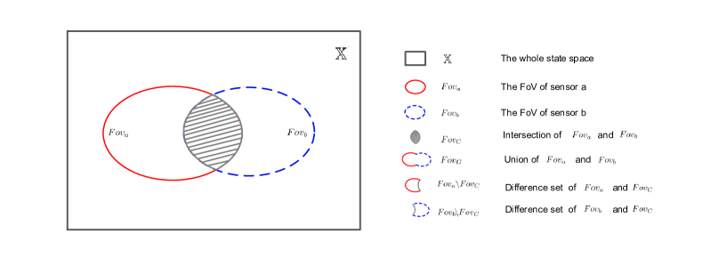
Figure 2: The relationship between FoVs involved in Subsection II-D

For agents working independently, the multi-object density $\pi_{i,ou}(X\cap(\mathbb{X}\backslash Fov_{i})|Fov_{i})$ is irrelevant since, usually, the region outside the FoV is not of interest and object tracks outside the FoV will not be displayed.

However, the objective of a sensor network is actually to surveil a much larger region of interest than the one that can be covered by an individual agent, through the cooperation of multiple agents with partially/non-overlapping FoVs. To this end, the fusion of multiple posteriors of individual agents is carried out at each time step, in order to get an average multi-object posterior that hopefully integrates information of all objects within the union of the individual FoVs. Employing the GCI rule and applying (15), the fusion of multi-object posteriors of sensors $a$ and $b$ yields:

$$\begin{split}\overline{\pi}(X)&\propto\pi_{a}(X)^{\omega_{a}}\,\pi_{b}(X)^{\omega_{a}}\\ &=\pi_{a,in}(X\cap Fov_{a})^{\omega_{a}}\pi_{a,ou}(X\cap(\mathbb{X}\backslash Fov_{a})|X\cap Fov_{a})^{\omega_{a}}\\ &\times\pi_{b,in}(X\cap Fov_{b})^{\omega_{b}}\pi_{b,ou}(X\cap(\mathbb{X}\backslash Fov_{b})|X\cap Fov_{b})^{\omega_{b}}\\ \end{split}$$ (16)

As can be seen from (16), the posteriors $\pi_{i,ou}(X\cap(\mathbb{X}\backslash Fov_{i})|X\cap Fov_{i})$ outside the FoV of each individual agent are involved in the fusion, and hence have a substantial impact on the fusion result.

Next in this section, we will analyse two usual implementations of GCI fusion relative to two different forms of $\pi_{i,ou}(X\cap(\mathbb{X}\backslash Fov_{i})|X\cap Fov_{i})$, and the corresponding impact on the fusion result.

III-1 Form-I - Missing objects outside the common FoV

The posterior of each individual agent has a tiny yes-probability [21] outside the FoV (corresponding to a no-object probability close to $1$), i.e.,

$$\pi_{i,ou}(X\cap\left(\mathbb{X}\backslash Fov_{i}\right)=\emptyset|X\cap Fov_{i})\approx 1,~{}~{}i=a,b.$$ (17)

Remark 3.

Note that the yes-probability of a given region represents the probability that the number of objects existing within the region is non-zero.

This usually occurs in the local filtering when :

• the survival probability is null outside the local FoV, i.e.,

  $$P_{S}(x)=0,\forall x\in\mathbb{X}\backslash Fov_{i};$$

• and/or the observation model does not properly take into account the fact that sensors cannot receive object measurements outside the FoV. For example, a sufficiently large detection probability outside the FoV is adopted, i.e., $P_{D}(x)=P_{D},\forall x\in\mathbb{X}\backslash Fov_{i}$.

Proposition 3.

Consider the GCI fusion of $\pi_{a}(\cdot)$ and $\pi_{b}(\cdot)$, i.e., $\overline{\pi}(\cdot)$ and its decomposition according to Proposition 2 by setting $\mathbb{V}=Fov_{C}$ and $\mathbb{W}=\mathbb{X}\backslash Fov_{C}$, i.e.,

$$\begin{split}&\overline{\pi}(X)=\overline{\pi}_{co}(X\cap Fov_{C})\,\overline{\pi}_{nc}(X\cap\left(\mathbb{X}\backslash Fov_{C}\right)|X\cap Fov_{C})\end{split}$$ (18)

where $Fov_{C}=Fov_{a}\cap Fov_{b}$ is the common FoV of agents $a$ and $b$. Then if

$$\pi_{i,ou}(X\cap\left(\mathbb{X}\backslash Fov_{i}\right)=\emptyset|X\cap Fov_{i})\to 1,~{}~{}i=a,b,$$ (19)

the following holds:

$$\overline{\pi}_{nc}(X\cap\left(\mathbb{X}\backslash Fov_{C}\right)=\emptyset|X\cap Fov_{C})\to 1.$$ (20)

Proof: see Section III of the supplemental materials. ∎

In particular, Proposition 3 indicates that, if $\pi_{i,ou}(X\cap\left(\mathbb{X}\backslash Fov_{i}\right))$ takes Form I, i.e., (19), then after fusion, only the existence of objects within the common FoV of sensors can be declared, while the objects outside $Fov_{C}$ are lost, since the corresponding no-object probability is close to 1.

This behavior is due to the fact that, even if each agent has no sensing ability for objects outside its FoV, it becomes too much overconfident to infer that “the object does not exist”. As a result, (19) is unreasonable and represents the main reason why standard GCI fusion can lose objects outside the common FoV.

III-2 Form-II - Biased estimation of objects outside the common FoV

The posterior of each agent outside the FoV is the prediction of the prior density. This occurs if

• $P_{S}(x)=P_{S},\forall x\in\mathbb{X}\backslash Fov_{i}$ (where $P_{S}$ is a value close to 1);

• the FoV is properly modelled, i.e. $P_{D}(x)=0$ for all $x\in\mathbb{X}\backslash Fov_{i}$.

Notice that $P_{D}(x)=0,\forall x\in\mathbb{X}\backslash Fov_{i}$, can be used in combination with any observation model, meaning that the sensor has null probability to receive observations of objects outside $Fov_{i}$. With this respect, the multi-object likelihood can be further represented by

$$\begin{split}g(Z_{i}|X)=&g(Z_{i}|X\cap Fov_{i},X\cap(\mathbb{X}\backslash Fov_{i})\\ =&g(Z_{i}|X\cap Fov_{i}).\end{split}$$ (21)

where the second equality in (21) is obtained since observations are independent of objects outside $Fov_{i}$.

Suppose that the prediction density on the space $\mathbb{X}$ at the current time step is as follows,

$$\pi_{i}^{-}(X)=\pi_{i,in}^{-}(X\cap Fov_{i})\pi_{i,ou}^{-}(X\cap(\mathbb{X}\backslash Fov_{i})|X\cap Fov_{i}).$$ (22)

According to the Bayes rule [21], the posterior is then computed by

$$\begin{split}&\pi_{i}(X|Z_{i})\propto\pi^{-}_{i,in}(X)g(Z_{i}|X)=\\ &\pi^{-}_{i,in}(X\!\cap\!Fov_{i})g(Z_{i}|X\cap Fov_{i})\pi^{-}_{i,ou}(X\!\cap\!(\mathbb{X}\backslash Fov_{i})|X\cap\!Fov_{i}).\end{split}$$ (23)

Eq. (23) suggests that the update procedure is only performed with the posterior within the FoV, while the posterior outside the FoV is just the prediction from the previous time step. Moreover, since the survival probability outside the FoV is close to 1, predicted kinematic states of objects outside the FoV are just obtained from the prior kinematic states exploiting the dynamic motion model, and such objects inherit the existence probabilities from the prior density. In fact, a common situation is that an object moves outside the FoV of a given agent for a long time so that the corresponding posterior is predicted for multiple steps ahead which, in turn, produces larger and larger estimation biases over time. Then, after fusion with posteriors from other agents, the resulting fused density also inherits the estimation biases, thus implying deteriorated fusion performance.

IV Principled fusion rule for multi-view multi-agent system

As we have analyzed in Section III, the misbehaviour of standard GCI fusion is due to the inconsistency of the local multi-object densities outside the FoV. In this section, a consistent multi-object posterior is constructed, so that the density within the FoV follows the marginal posterior provided by local filtering, while the density outside the FoV adopts a multi-object uninformative prior. Then, on the basis of this decomposition, we further propose a principled rule to handle multi-agent multi-view fusion.

IV-A Principled fusion rule

IV-A1 Form III - Consistent marginal density outside the local FoV

Proposition 4.

Multi-object uninformative density over a bounded state space – Let $\digamma$ be the family of multi-object densities over a state space $\zeta$ of finite volume $V(\zeta)$. Then, a multi-object uninformative density over $\digamma$ can be defined as follows

$$\pi_{ui}(X)=\left\{\begin{array}[]{ll}\ \dfrac{1}{\sum_{m=0}^{n_{\text{max}}}\frac{[V(\zeta)]^{m}}{m!}},&\text{if }X\in\mathcal{F}(\zeta)\vspace{2mm}\\ \ 0,&\text{otherwise}\end{array}\right.$$ (24)

where $n_{\text{max}}$ is the maximum cardinality, and if $n_{\text{max}}\rightarrow+\infty$,

$$\pi_{ui}(X)=\left\{\begin{array}[]{ll}\ e^{-V(\zeta)},&\text{if }X\in\mathcal{F}(\zeta)\\ \ 0,&\text{otherwise.}\end{array}\right.$$ (25)

Proof: see Section IV of the supplemental materials. ∎

Remark 4.

The multi-object uninformative density (24) defines an i.i.d. cluster process

$$\pi_{ui}(X)=n!\,\rho(n)\,[p]^{X},$$ (26)

with cardinality distribution

$$\rho(n)=\frac{\frac{[V(\zeta)]^{n}}{{n!}}}{\sum_{m=0}^{n_{\text{max}}}\frac{[V(\zeta)]^{m}}{m!}},$$ (27)

and location density

$$p(x)=\frac{1}{V(\zeta)}.$$ (28)

IV-A2 Principled fusion for the two-agent case

Let us again consider, without loss of generality, a network with two agents $a$ and $b$. Let $\pi_{a,ui}$ and $\pi_{b,ui}$ denote multi-object uninformative densities on the state spaces $Fov_{a}\backslash Fov_{C}$ and $Fov_{b}\backslash Fov_{C}$, respectively. Adopting $\pi_{a,ui}$ and $\pi_{b,ui}$ as densities outside the local FoVs of agents $a$ and $b$, the posteriors of such agents both defined on the global FoV $Fov_{G}=Fov_{a}\cup Fov_{b}$ turn out to be

$$\pi_{a}(X)=\pi_{a}(X\cap Fov_{a})\,\pi_{a,ui}(X\cap(Fov_{b}\backslash Fov_{C}))$$ (29)

and

$$\pi_{b}(X)=\pi_{b}(X\cap Fov_{b})\,\pi_{b,ui}(X\cap(Fov_{a}\backslash Fov_{C})).$$ (30)

Remark 5.

Please note that $\pi_{i,ui}$ is not a posterior, but actually a diffuse prior. However, considering that $\pi_{i,in}(X\cap Fov_{i})$ is the marginal density of the posterior, with a little abuse of terminology, we also call (29) and (30) as posteriors of agents $a$ and $b$.

Remark 6.

$\pi_{a}$ and $\pi_{b}$ both are considered to be defined on $Fov_{G}$. The densities outside the global FoV, $Fov_{G}$, i.e., $\pi_{i}(X\cap\mathbb{X}\backslash Fov_{G}|X\cap Fov_{G})$ are neglected, since the corresponding region $\mathbb{X}\backslash Fov_{G}$ is outside the FoVs of both $a$ and $b$, wherein both $a$ and $b$ cannot get valid measurements.

Further, based on (14), $\pi_{i}(X\cap Fov_{i})$ can be decomposed as

$$\begin{split}&\pi_{i}(X\cap Fov_{i})\!=\pi_{i,co}(X\cap Fov_{C})\times\\ &\,\,\,\,\,\,\,\pi_{i,nc}(X\cap(Fov_{i}\backslash Fov_{C})|X\!\cap\!Fov_{C}),~{}~{}i=a,b\end{split}$$ (31)

where $\pi_{i,co}(X\cap Fov_{C})$ and $\pi_{i,nc}(X\cap(Fov_{i}\backslash Fov_{C})|X\!\cap\!Fov_{C})$ describe the statistics of objects within the common FoV and, respectively, non-common (exclusive) FoV of agent $i$.

According to the GCI rule, the fusion of $\pi_{a}(X)$ and $\pi_{b}(X)$ yields:

$$\begin{split}\overline{\pi}(X)\propto&{\pi_{a,co}(X\cap Fov_{C})}^{\omega_{a}}{\pi_{b,co}(X\!\cap\!Fov_{C})}^{\omega_{b}}\times\\ &\pi_{a,nc}(X\!\cap\!(Fov_{a}\backslash Fov_{C})|X\!\cap Fov_{C})^{\omega_{a}}\times\\ &{\pi_{b,ui}(X\cap(Fov_{a}\backslash Fov_{C}))}^{\omega_{b}}\times\\ &{\pi_{a,ui}(X\!\cap\!Fov_{b}\backslash Fov_{C})}^{\omega_{a}}\times\\ &{\pi_{b,nc}(X\!\cap\!(Fov_{b}\backslash Fov_{C})|X\!\cap\!Fov_{C})}^{\omega_{b}},\end{split}$$ (32)

where $\omega_{i}\in[0,1]$, for $i\in\{a,b\}$, and $\omega_{a}+\omega_{b}=1$.

Recall that the normalization of the fusion weights (i.e., $\omega_{a}+\omega_{b}=1$) is to avoid the double counting of common information of different agents [1, 7]. Looking at (32), the common information between agents $a$ and $b$ can only be on $X\cap Fov_{C}$ which are the object states within the common FoV of agents $a$ and $b$. As for the exclusive object states $X\cap\left(Fov_{a}\backslash Fov_{C}\right)$ and $X\cap\left(Fov_{b}\backslash Fov_{C}\right)$, they are only observed by a single agent so that the corresponding density of the other agent used for fusion is a multi-object uninformative density, implying no common information between the two agents. Hence, if fusion weights $\omega_{a}<1$ and/or $\omega_{b}<1$ are applied also to the exclusive densities $\pi_{a,nc},\pi_{a,ui}$ and/or $\pi_{b,nc},\pi_{b,ui}$ in (32), an under-confidence problem occurs.

Hence, to avoid this problem, a better alternative for the fusion with respect to $X\cap\left(Fov_{a}\backslash Fov_{C}\right)$ or $X\cap\left(Fov_{b}\backslash Fov_{C}\right)$ is to perform Bayesian rule [21], that amounts to power-raising posteriors of different agents with unit weights $\omega_{a}=\omega_{b}=1$. The rationale is that, as a result, the corresponding fusion becomes (33).

$$\begin{split}\overline{\pi}(X)&\propto\underbrace{{\pi_{a,co}(X\cap Fov_{C})}^{\omega_{a}}{\pi_{b,co}(X\cap Fov_{C})}^{\omega_{b}}}_{\text{Fusion on }Fov_{C}}\times\underbrace{{\pi_{a,ui}(X\cap Fov_{b}\backslash Fov_{C})}{\pi_{b,nc}(X\cap(Fov_{b}\backslash Fov_{C})|X\!\cap\!Fov_{C})}}_{\text{Fusion on the difference set }Fov_{b}\backslash Fov_{C}}\\ &\,\,\,\,\,\,\,\,\,\,\,\,\,\,\,\,\,\,\,\,\,\,\,\,\,\,\,\,\,\,\,\,\,\,\,\,\,\,\,\,\,\times\underbrace{\pi_{a,nc}(X\cap(Fov_{a}\backslash Fov_{C})|X\!\cap\ Fov_{C}){\pi_{b,ui}(X\cap(Fov_{a}\backslash Fov_{C}))}}_{\text{Fusion on the difference set }Fov_{a}\backslash Fov_{C}}\end{split}$$ (33)

Exploiting the Bayesian-operator invariance of multi-object uninformative densities, after normalization (33) can be further expressed as (34),

$$\!\!\!\!\overline{\pi}(X)=\underbrace{\overline{\pi}_{co}(X\cap Fov_{C})}_{\text{GCI}}\times\underbrace{{\pi_{a,nc}(X\cap(Fov_{a}\backslash Fov_{C})|X\cap Fov_{C})}}_{\text{Bayesian-operator invariance}}\times\underbrace{{\pi_{b,nc}(X\cap(Fov_{b}\backslash Fov_{C})|X\cap Fov_{C})}}_{\text{Bayesian-operator invariance}}$$ (34)

where, $\forall X\in\mathcal{F}(Fov_{C})$,

$$\overline{\pi}_{co}(X)=\frac{{\pi_{a,co}(X)}^{\omega_{a}}\,{\pi_{b,co}(X)}^{\omega_{b}}}{\int{\pi_{a,co}(X)}^{\omega_{a}}\,{\pi_{b,co}(X)}^{\omega_{b}}\delta X}.$$ (35)

The proposed fusion rule (34)-(35) is referred to hereafter as Bayesian-operator InvaRiance on Difference-sets (BIRD) where difference-sets refer to $Fov_{b}\backslash Fov_{C}$ and $Fov_{b}\backslash Fov_{C}$.

Remark 7.

The proposed BIRD fusion is in the same spirit of the split CI fusion [26] that performs CI fusion for the unknown correlated components, while applies the Kalman filter to the known independent components.

For a single agent $i$, which is not to get object observations outside its individual FoV, only the posterior $\pi_{i}(X\cap Fov_{i})$ is informative and reliable; accordingly, only detections/estimates of objects moving within $Fov_{i}$ can be provided. However, by employing the proposed BIRD fusion in (34)-(35), a reliable and informative density $\overline{\pi}(X)$ over the global FoV is obtained, so that detections/estimates of all objects within the union of individual FoVs can be provided. Furthermore, the fused density achieves maximum information gain from the local posteriors within the common FoV, and also preserves, in the exclusive FoV, sufficient and valid information provided by the observing agent.

IV-A3 Multi-agent case

The BIRD fusion approach, presented above for $N_{s}=2$ agents, can be easily extended to the case of $N_{s}>2$ agents by sequentially applying the pairwise fusion (33)-(34) $N_{s}-1$ times. The same sequential fusion strategy has already been adopted for standard GCI fusion with CPHD [1] and, respectively, MB filters [8].

The pseudocode of sequential BIRD fusion is given in Algorithm 1, for which the following comments are in order.

INPUT: Local posterior $\pi_{i}$ and field-of-view $Fov_{i}$ of any agent $i\in\{1,2,\dots,N_{s}\}$ involved in the fusion;

OUTPUT: Fused density $\overline{\pi}$ and domain of definition $\overline{Fov}$;

function $(\overline{\pi},\overline{Fov})=\mathfrak{F}$($\{(\pi_{1},Fov_{1}),\cdots,(\pi_{N_{s}},Fov_{N_{s}})\}$

for $j=2:N_{s}$

 do

      Calculate the common FoV: $Fov_{C}=Fov_{1}\cap Fov_{j}$;

       Calculate the marginal densities $\pi_{1,co}(X\cap Fov_{C})$ and $\pi_{j,co}(X\cap Fov_{C})$ according to (9);

       Calculate the conditional densities $\pi_{1,nc}(X\cap(Fov_{1}\backslash Fov_{C})|X\cap Fov_{C})$ and $\pi_{j,nc}(X\cap(Fov_{i}\backslash Fov_{C})|X\cap Fov_{C})$ according to (11);

       Compute the fused density according to (34) and (35):

$$\begin{split}\overline{\pi}(X):=&\overline{\pi}_{co}(X\cap Fov_{C})\\ &\pi_{1,nc}(X\cap(Fov_{1}\backslash Fov_{C})|X\cap Fov_{C})\times\\ &{\pi_{i,nc}(X\cap(Fov_{j}\backslash Fov_{C})|X\cap Fov_{C})};\end{split}$$

      $\overline{Fov}:=Fov_{1}\cup Fov_{j}$;

       $\pi_{1}:=\overline{\pi}$;

       $Fov_{1}:=\overline{Fov}$;

end for

return: $\overline{\pi}$ and $\overline{Fov}$.

Algorithm 1 Sequential BIRD fusion

• After performing fusion $N_{s}-1$ times sequentially, the final fused density $\overline{\pi}(X)$ will be informative over the global Fov of the sensor network, i.e., $\overline{Fov}=Fov_{G}$, integrating object information of all agents.

• Let $\{A_{1},\cdots,A_{N}\}$ provide a partition of the global FoV $Fov_{G}$, where each $A_{j}$ is the intersection of the FoVs of all agents $i$ that can illuminate the region $A_{j}$, i.e.,

  $$A_{j}=\bigcap_{i:A_{j}\subseteq Fov_{i}}Fov_{i}.$$ (36)

  After the $N_{s}-1$ pairwise fusion steps, for each $A_{j}$, the fusion is only performed with all agents that can illuminate $A_{j}$. As for other sensors which cannot illuminate $A_{j}$, since multi-object uninformative densities are considered in the fusion, there is no impact on the fusion result.

The above two points ensure that the fused density integrates the most appropriate amount of information from all agents over the global FoV. To further clarify the aforementioned observations, we give hereafter an example relative to three agents.

Example 1.

Let us consider fusion of three densities $\pi_{1}$, $\pi_{2}$, $\pi_{3}$ provided by three agents with respective fields-of-view $Fov_{1}$, $Fov_{2}$, $Fov_{3}$. The global FoV is partitioned into $6$ regions denoted by $A_{i}$ ($i=1,\cdots 6$) as shown in Fig. 3.

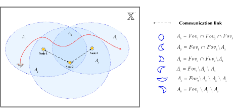
Figure 3: Division of the global FoV of the sensor network.

By adopting the sequential pairwise strategy, fusion is first performed between $\pi_{1}$ and $\pi_{2}$ according to (34), resulting into

$${\small{\begin{split}\!\!&\overline{\pi}_{1,2}(X)\\ \!\!\propto&\pi_{1,co}(X\cap\left(A_{2}\cup A_{3}\right))^{\omega}\pi_{2,co}(X\cap\left(A_{2}\cup A_{3}\right))^{1-\omega}\times\\ &\pi_{1,nc}(X\cap A_{1}|\left(A_{2}\cup A_{3}\right))\pi_{2,nc}(X\cap\left(A_{4}\cup A_{5}\right)|\left(A_{2}\cup A_{3}\right))\end{split}}}$$ (37)

After normalization, we get a fused density $\overline{\pi}_{1,2}(X)$ defined on

$$Fov_{1}\cup Fov_{2}=A_{1}\cup A_{2}\cup A_{3}\cup A_{4}\cup A_{5}.$$

Then, fusion is further performed between $\overline{\pi}_{1,2}(X)$ and $\pi_{3}(X)$. According to (34), the final fused density yields:

$${\small{\begin{split}&\overline{\pi}_{1,2,3}(X)\\ \propto&\overline{\pi}_{1,2,c}(X\cap\left(A_{3}\cup A_{5}\right))^{\omega}\pi_{3,c}(X\cap\left(A_{3}\cup A_{5}\right))^{(1-\omega)}\times\\ &\overline{\pi}_{1,2,nc}(X\cap\left(A_{1}\cup A_{2}\cup A_{4}\right)|X\cap\left(A_{3}\cup A_{5}\right))\times\\ &\pi_{3,nc}(X\cap A_{6}|X\cap\left(A_{3}\cup A_{5}\right))\end{split}}}$$ (38)

After normalization of (38), the final fused density $\overline{\pi}_{1,2,3}(X)$ is defined on the global Fov, i.e. $\overline{Fov}=\cup_{i=1}^{6}A_{i}=Fov_{G}$, integrating object information of all three agents.

Specifically, observing (37) and (38):

• for the region $A_{3}$ illuminated by all three agents, the fusion actually involves all the three densities;

• for the regions $A_{2}$ and $A_{5}$ illuminated by only two agents, the fusion involves the two densities of such agents;

• for the regions $A_{1}$, $A_{4}$ and $A_{6}$ illuminated by a single agent, no fusion is actually performed but the corresponding density of the illuminating agent is preserved.

IV-B Implementation of BIRD fusion

This subsection provides the specific implementation of BIRD fusion, from the perspective of local filtering and consensus-based distributed fusion.

IV-B1 Local filtering for BIRD fusion

Observing the proposed fusion formula (34), only the marginal density with respect to $Fov_{i}$ of each agent’s posterior, i.e. $\pi_{i}(X\cap Fov_{i})$, is used for fusion. This is consistent with the fact that the local filter can only provide valid updates to the prior within the local FoV. As a result, before BIRD fusion, the marginal posterior $\pi_{i}(X\cap Fov_{i})$ is calculated first. Hence, it does not matter how the probabilities of survival and detection are chosen outside the local FoV for local filtering, which further demonstrates the robustness of the proposed fusion.

IV-B2 Consensus-based distributed fusion

The fusion formula (34) can be readily applied to the centralized case by adopting the sequential fusion given in Algorithm 1. However, how to utilize the fusion formula in a fully distributed way is not obvious. In this subsection, we discuss the application of (34) to the distributed peer-to-peer setting.

In a distributed sensor network, each agent has also limited communication capability and hence, at each time step, can only receive the posteriors of its neighbours. In order to make each agent share the global information of the whole network, a consensus approach [27, 1] is usually adopted. The core idea of consensus-based distributed fusion is that, at each time instant $k$, the collective fusion can be approximated by iterating regional fusions, called consensus steps, among neighboring nodes. More precisely, at each sampling interval $k$, a certain number of consensus steps, say $L$, is performed. Let us denote by $\pi_{i}^{\ell}(X)$ the density of agent $i$ at (time $k$, not indicated for the sake of simplicity, and) consensus step $\ell$. Then, by applying consensus to the proposed enhanced fusion rule (33), we obtain the recursive algorithm, for each $\ell=1,\cdots,L$,

$$\begin{split}(\pi_{i}^{(\ell)},Fov^{\ell})=\mathfrak{F}(\{(\pi_{j}^{(\ell-1)},Fov^{(\ell-1)}\}_{j\in\mathcal{N}_{i}}),\forall i\in\mathcal{N},\end{split}$$ (39)

where $\pi_{i}^{(0)}=\pi_{i}$, $Fov^{(0)}=Fov_{i}$, $i\in\mathcal{N}$, $\mathfrak{F}(\cdot)$ is given in Algorithm I.

According to the proposed fusion rule, the actual FoV of each agent is extended with the progression of consensus steps. After a certain number of steps (which is at least equal to the network diameter), each agent can share the global FoV and all information of the other agents.

The pseudocode of the consensus-based distributed BIRD fusion is given in Algorithm 2.

INPUT: Local posterior $\pi_{j}$ and field-of-view $Fov_{j}$ of each agent $j\in\mathcal{N}_{i}$; number of consensus steps $L$;

OUTPUT: Consensus-based fused density $\pi_{i}^{(L)}$ and domain of definition $Fov_{i}^{(L)}$;

function $\mathfrak{F}_{con}$($\{\left(\pi_{j},Fov_{j}\right)\}_{j\in\mathcal{N}_{i}}$)

Perform the initialization:

$$\pi_{i}^{(0)}:= \pi_{i},$$

$$Fov_{i}^{(0)}:= Fov_{i}$$

for $\ell=1:L$ do

      Exchange posteriors with neighbours;

       Perform the sequential BIRD fusion given in Algorithm I $(\pi_{i}^{(\ell)},Fov_{i}^{(\ell)})=\mathfrak{F}(\{(\pi_{j}^{(\ell-1)},Fov_{j}^{(\ell-1)})\}_{j\in\mathcal{N}_{i}})$

end for

return: $\left(\pi_{i}^{(L)},Fov_{i}^{(L)}\right)$.

Algorithm 2 Consensus based BIRD fusion performed by agent $i\in\mathcal{N}$.

V BIRD fusion of Poisson RFSs

For the subsequent developments, the attention is devoted to specific RFSs called Poisson, more precisely Poisson point processes [28] or multi-object Poisson processes[21], that play a fundamental role in PHD filtering [21, 29].

V-A Decomposition and union of Poisson RFSs

We will first derive in Proposition 5 the marginal density of a Poisson RFS, based on which the decomposition of a Poisson RFS with respect to disjoint subspaces in the form of (14) will be given in Proposition 6. Finally, Proposition 7 will show that for any two Poisson RFSs defined on disjoint spaces, their union is another Poisson RFS defined on the union of such spaces.

Proposition 5.

Let us consider a Poisson RFS on $\mathbb{X}$ with density

$$\pi(X)=[\lambda]^{|X|}\,\exp(-\lambda)\,p^{X},$$ (40)

where $p^{X}\triangleq\prod_{x\in X}p(x)$ with $p^{\emptyset}\triangleq 1$ by convention. Then, $X_{W}=X\cap\mathbb{W}$, with $\mathbb{W}\subseteq\mathbb{X}$, is also a Poisson RFS with marginal density

$$\pi_{W}(X)=[\lambda K_{W}]^{|X|}\exp(-\lambda K_{W})p_{W}^{X}$$ (41)

where

$$p_{W}(x)\triangleq \frac{1_{\mathbb{W}}(x)p(x)}{K_{W}}$$ (42)

$$K_{W}\triangleq \int_{\mathbb{W}}p(x)dx$$ (43)

Further, $X_{V}=X\backslash X_{W}$ defined on $\mathbb{V}=\mathbb{X}\backslash\mathbb{W}$ and conditioned on $X_{W}$, is also a Poisson RFS, with the conditional density

$$\pi_{V}(X^{\prime}|X)=\pi_{V}(X^{\prime})=[\lambda K_{V}]^{|X^{\prime}|}\,\exp(-\lambda K_{V})\,p_{V}^{X^{\prime}}$$ (44)

where

$$p_{V}(x)\triangleq \frac{1_{\mathbb{V}}(x)p(x)}{K_{V}}$$ (45)

$$K_{V}\triangleq \int_{\mathbb{V}}p(x)dx=1-K_{W}$$ (46)

Proof: see Subsection V of the supplemental materials . ∎

Proposition 6.

(Decomposition) Let us consider a Poisson RFS on $\mathbb{X}$ with density

$$\pi(X)=[\lambda]^{|X|}\exp(-\lambda)p^{X}$$ (47)

and an arbitrary partition $\mathbb{X}=\mathbb{W}\uplus\mathbb{V}$. Then, the density can be factored as follows:

$$\pi(X)=\pi_{W}(X\cap\mathbb{W})\,\pi_{V}(X\cap\mathbb{V})$$ (48)

where: $\pi_{W}(X)$ is a Poisson RFS density on $\mathbb{W}$ with parameter pair $(\lambda K_{W},p_{W}(x))$; $\pi_{V}(X)$ is a Poisson RFS density on $\mathbb{V}$ with parameter pair $(\lambda K_{V},p_{V}(x))$; $p_{W},K_{W},p_{V},K_{V}$ are given by (42), (43), (45) and (46), respectively.

Proof: Proposition 6 is a direct consequence of Proposition 5, considering that, by dividing the state space into disjoint subspaces, one can always write a Poisson RFS as union of independent Poisson RFSs on such disjoint subspaces. It is, therefore, a special property of the Poisson RFS family. ∎

Proposition 7.

(Union) Let us consider Poisson RFSs $X_{W}$ and $X_{V}$ defined on disjoint state spaces $\mathbb{W}$ and $\mathbb{V}$ (i.e., $\mathbb{W}\cap\mathbb{V}=\emptyset$), with densities $\pi_{W}(\cdot)$ and $\pi_{V}(\cdot)$ given by

$$\pi_{W}(X)= [\lambda_{W}]^{|X|}\exp(-\lambda_{W})p_{W}^{X}$$ (49)

$$\pi_{V}(X)= [\lambda_{V}]^{|X|}\exp(-\lambda_{V})p_{V}^{X}.$$ (50)

Then, the union of $X_{W}$ and $X_{V}$, i.e. $X=X_{W}\cup X_{V}$, turns out to be a Poisson RFS on state space $\mathbb{X}=\mathbb{W}\cup\mathbb{V}$, with density

$$\begin{split}\pi(X)=&[\lambda]^{|X|}\exp(-\lambda)p^{X}\end{split}$$ (51)

where

$$\lambda= \lambda_{W}+\lambda_{V}$$ (52)

$$p(x)= \frac{\lambda_{W}}{\lambda}p_{W}(x)+\frac{\lambda_{V}}{\lambda}p_{V}(x)$$ (53)

Proof: see Subsection VI of the supplemental materials. ∎

V-B Fusion formulas of Poisson RFSs

Now, the fusion of Poisson posteriors using the BIRD rule (34) is detailed. For the sake of simplicity and without loss of generality, the case of two agents will be dealt with, recalling that more agents can be anyway handled by sequential pairwise fusion steps according to Algorithm 1, or the consensus based distributed fusion according to Algorithm 2. Hence, let us assume that agents $a$ and $b$ have Poisson posteriors, defined on $Fov_{a}$ and $Fov_{b}$, of the form

$$\pi_{i}(X)=[\lambda_{i}]^{|X|}\,\exp(-\lambda_{i})\,p_{i}^{X},~{}~{}~{}i=a,b$$ (54)

Notice that the Poisson RFS (54) is completely characterized by the parameter pair $(\lambda_{i},p_{i})$ [21].

The BIRD fusion of $\pi_{a}$ and $\pi_{b}$ can, therefore, be performed via the following three-step procedure.

STEP 1: Perform the decomposition of the posteriors $(\lambda_{i},p_{i}(x))$ on $Fov_{i}$ of agents $i=a,b$ by dividing the state space into disjoint subsets, $Fov_{C}$ and $Fov_{i}\backslash Fov_{C}$, i.e.

$$\pi_{i}(x)=\pi_{i,co}(X\cap Fov_{C})\,\pi_{i,nc}(X\cap(Fov_{i}\backslash Fov_{C})).$$ (55)

According to Proposition 4 and proposition 5, $\pi_{i,co}$ and $\pi_{i,nc}$ are both Poisson parameterized by $(\lambda_{i,co},p_{i,co}(x))$ and $(\lambda_{i,nc},p_{i,nc}(x))$, respectively, with

$$\lambda_{i,co}= \lambda_{i}K_{i,co}$$ (56)

$$K_{i,co}= \int_{Fov_{C}}p_{i}(x)dx$$ (57)

$$p_{i,co}(x)= \frac{1_{Fov_{C}}(x)p_{i}(x)}{K_{i,co}}$$ (58)

$$\lambda_{i,nc}= \lambda_{i}K_{i,nc}$$ (59)

$$K_{i,nc}= \int_{Fov_{i}\backslash{Fov_{C}}}p_{i,nc}(x)dx$$ (60)

$$p_{i,nc}(x)= \frac{1_{Fov_{i}\backslash Fov_{C}}(x)p_{i,nc}(x)}{K_{i,nc}}$$ (61)

STEP 2: Compute the fused density over the common FoV, $Fov_{C}$, namely the GCI fusion of $\pi_{a,co}(X)$ and $\pi_{b,co}(X)$ (both defined on the common field-of-view $Fov_{C}$.

Since $\pi_{a,co}(X)$ and $\pi_{b,co}(X)$ are both Poisson, as proved in [6], the fused density $\overline{\pi}_{co}$ is also Poisson, parameterized by $(\overline{\lambda}_{co},\overline{p}_{co})$ where

$$\overline{\lambda}_{co}= \lambda_{a,co}^{\omega_{a}}\,\lambda_{b,co}^{\omega_{b}}\,\overline{K}_{co}$$ (62)

$$\overline{p}_{co}= \frac{1_{Fov_{C}}(x)\,p_{a,co}(x)^{\omega_{a}}\,p_{b,co}(x)^{\omega_{b}}}{\overline{K}_{co}}$$ (63)

$$\overline{K}_{co}= \int_{Fov_{C}}p_{a,co}^{\omega_{a}}(x)\,p_{b,co}^{\omega_{b}}(x)\,dx$$ (64)

STEP 3: According to (34), compute the global fused density $\overline{\pi}(X)$ over the global FoV, i.e.,

$$\begin{split}Fov_{G}=&(Fov_{a}\backslash Fov_{C})\cup Fov_{C}\cup(Fov_{b}\backslash Fov_{C})\\ =&Fov_{a}\cup Fov_{b}.\end{split}$$ (65)

This step amounts to performing disjoint union of three Poisson RFSs with densities $\pi_{i,nc}$ (on state space $Fov_{i}\backslash Fov_{C}$), $i\in\{a,b\}$, and $\overline{\pi}_{co}(X)$ (on state space $Fov_{C}$). Applying Proposition 7 twice, the global fused density $\overline{\pi}$ yields another Poisson RFS parameterized by $(\overline{\lambda},\overline{p})$ with

$$\overline{p}(x)\triangleq \frac{\overline{\lambda}_{co}}{\overline{\lambda}}\,\overline{p}_{c}(x)+\frac{\lambda_{a,nc}}{\overline{\lambda}}\,p_{a,nc}(x)+\frac{\lambda_{b,nc}}{\overline{\lambda}}\,p_{b,nc}(x)$$ (66)

$$\overline{\lambda}= \overline{\lambda}_{co}+\lambda_{a,nc}+\lambda_{b,nc}$$ (67)

V-C Gaussian mixture implementation

Let us again consider agents $a$ and $b$ with Poisson posteriors. As mentioned in Subsection IV-B, before BIRD fusion, the marginal density with respect to the local FoV, i.e. $\pi_{i}(X\cap Fov_{i})$ is calculated. According to Proposition 5, the resulting marginal posterior is also Poisson characterized by parameter pairs $(\lambda_{i},p_{i})$, $i\in\{a,b\}$, with location densities represented in bounded GM form as

$$p_{i}(x)=\sum_{j=1}^{N_{G,i}}\alpha_{i}^{(j)}\,\mathcal{N}(x;\hat{x}_{i}^{(j)},P_{i}^{(j)})\,1_{Fov_{i}}(x),~{}~{}~{}i=a,b.$$ (68)

Next, a step-by-step implementation of the proposed BIRD fusion is given as follows.

STEP 1: Given the GM form of $p_{i}(x)$ in (68), the parameters of $\pi_{i,nc}$ and $\pi_{i,nc}$ are computed as follows.

1) Calculation of $\lambda_{i,co}$: First, the calculation of $K_{i,co}$ is considered. According to (57), we have

$$\begin{split}K_{i,co}=&\int_{Fov_{C}}\sum_{j=1}^{N_{G,i}}\alpha^{(j)}_{i}\mathcal{N}(x;\hat{x}_{i}^{(j)},P_{i}^{(j)})\,dx\\ =&\sum_{j=1}^{N_{G,i}}\alpha^{(j)}_{i}c_{i}^{(j)}(Fov_{C})\end{split}$$ (69)

where

$$c_{i}^{(j)}(Fov_{C})=\int_{Fov_{C}}\mathcal{N}(x;\hat{x}_{i}^{(j)},P_{i}^{(j)})\,dx.$$ (70)

Even though (70) is the integration of a Gaussian density, there is no closed-form expression for it. Hence, we provide a Monte Carlo (MC) approximation of $c^{(j)}_{i}{(Fov_{C})}$ as follows: draw $M^{(j)}_{i}$ samples $x^{(j,m)}_{i}$, for $m=1,\cdots,M_{i}^{(j)}$, from the Gaussian density $\mathcal{N}(x;\hat{x}_{i}^{(j)},P_{i}^{(j)})$, then $c_{i}^{(j)}(Fov_{C})$ can be approximated as

$$\begin{split}c^{(j)}_{i}{(Fov_{C})}=&\dfrac{1}{M_{i}^{(j)}}\,\sum_{m=1}^{M^{(j)}_{i}}1_{Fov_{C}}(x^{(j,m)}_{i}).\end{split}$$ (71)

Then, according to (69), the quantity $K_{i,co}$ can be approximated as

$$K_{i,co}=\sum_{j=1}^{N_{G,i}}\,\dfrac{\alpha_{i}^{(j)}}{M_{i}^{(j)}}\,\sum_{m=1}^{M^{(j)}_{i}}1_{Fov_{C}}(x^{(j,m)}_{i}).$$ (72)

As a result, according to (56), the parameter $\lambda_{i,co}$ can be computed by

$$\lambda_{i,co}=\lambda_{i}K_{i,co}=\lambda_{i}\sum_{j=1}^{N_{G,i}}\dfrac{\alpha^{(j)}_{i}}{M_{i}^{(j)}}\,\sum_{m=1}^{M^{(j)}_{i}}1_{Fov_{C}}(x^{(j,m)}_{i}).$$ (73)

2) Calculation of $p_{i,co}(x)$: According to (58) and the evaluated $K_{i,C}$ given in (72), the location density over $Fov_{C}$ is given by

$$p_{i,co}(x)=\sum_{j=1}^{N_{G,i}}\frac{\alpha_{i}^{(j)}}{K_{i,co}}\,\mathcal{N}(x;\hat{x}_{i}^{(j)},P_{i}^{(j)})\,1_{Fov_{C}}(x).$$ (74)

3) Calculation of $\lambda_{i,nc}$ and $p_{i,nc}(x)$: Given the evaluated $K_{i,c}$ in (72), the quantity $K_{i,nc}$ can be easily computed by

$$K_{i,nc}=1-K_{i,co}.$$ (75)

Further, similarly as for $p_{i,co}$, according to (61), $p_{i,nc}(x)$ is given by,

$$p_{i,nc}(x)\!\!=\!\!\sum_{j=1}^{N_{G,i}}\frac{\alpha_{i}^{(j)}}{K_{i,nc}}\,\mathcal{N}(x;\hat{x}_{i}^{(j)},P_{i}^{(j)})\,1_{Fov_{i}\backslash Fov_{C}}(x).$$ (76)

STEP 2: We first compute the numerator of the fused location density $\overline{p}_{co}(x)$. By substituting the GM forms of $p_{a,co}(x)$ and $p_{b,co}(x)$ in (74) into the numerator of (63), we get

$$\begin{split}&1_{Fov_{C}}(x)p_{a,co}(x)^{\omega_{a}}p_{b,co}(x)^{\omega_{b}}\\ =&1_{Fov_{C}}(x)\left[\sum_{j=1}^{N_{G,a}}\frac{\alpha_{a}^{(j)}}{K_{a,co}}\mathcal{N}(x;\hat{x}_{a}^{(j)},P_{a}^{(j)})1_{Fov_{C}}(x)\right]^{\omega_{a}}\times\\ &\left[\sum_{j=1}^{N_{G,b}}\frac{\alpha_{b}^{(j)}}{K_{b,co}}\mathcal{N}(x;\hat{x}_{b}^{(j)},P_{b}^{(j)})1_{Fov_{C}}(x)\right]^{\omega_{b}}.\end{split}$$ (77)

Notice that (77) involves exponentiation of a GM which, unfortunately, does not provide a GM in general. As suggested in [1], the following approximation is reasonable

$$\begin{split}&\left[\sum_{j=1}^{N_{G,i}}\frac{\alpha_{i}^{(j)}}{K_{i,co}}\mathcal{N}(x;\hat{x}_{i}^{(j)},P_{i}^{(j)})1_{Fov_{C}}(x)\right]^{\omega_{i}}\\ \cong&\sum_{j=1}^{N_{G,i}}\left(\frac{\alpha_{i}^{(j)}}{K_{i,co}}\right)^{\omega_{i}}\left[\mathcal{N}(x;\hat{x}_{i}^{(j)},P_{i}^{(j)})1_{Fov_{C}}(x)\right]^{\omega_{i}}\end{split}$$ (78)

as long as the Gaussian components of $p_{i,co}(x)$ are well separated relatively to their corresponding covariances. In case the components are not well separated, one can either perform merging before fusion (this is possible since, for a Poisson RFS, each location density $p_{i,co}(x)$ refers to a hypothetic single object) or use different approximations, e.g., by replacing the GM representation by a sigma-point approximation [30].

As a result, (77) can be further re-expressed as

$$\begin{split}&1_{Fov_{C}}(x)p_{a,co}(x)^{\omega_{a}}p_{b,co}(x)^{\omega_{b}}\\ =&\sum_{j=1}^{N_{G,a}}\!\sum_{j^{\prime}=1}^{N_{G,b}}\left(\frac{\alpha_{a}^{(j)}}{K_{a,co}}\right)^{\!\!\omega_{a}}\!\!\!\left(\frac{\alpha_{b}^{(j)}}{K_{b,co}}\right)^{\!\!\omega_{b}}\!\!\!\left[\mathcal{N}(x;\hat{x}_{a}^{(j)},P_{a}^{(j)})1_{Fov_{C}}(x)\right]^{\!\omega_{a}}\\ &\times\left[\mathcal{N}(x;\hat{x}_{b}^{(j^{\prime})},P_{b}^{(j^{\prime})})1_{Fov_{C}}(x)\right]^{\omega_{b}}1_{Fov_{C}}(x).\end{split}$$ (79)

Then, by exploiting some elementary operations on GMs [1], the numerator (79) can be rewritten as

$$\begin{split}&1_{Fov_{C}}(x)p_{a,co}(x)^{\omega_{a}}p_{b,co}(x)^{\omega_{b}}\\ =&\sum_{j=1}^{N_{G,a}}\sum_{j^{\prime}=1}^{N_{G,b}}\widetilde{\alpha}^{(j,j^{\prime})}\mathcal{N}(x;\hat{x}^{(j,j^{\prime})},P^{(j,j^{\prime})})\,1_{Fov_{C}}(x)\end{split}$$ (80)

where

$$P^{(j,j^{\prime})}= \left[\omega_{a}(P_{a}^{(j)})^{-1}+\omega_{b}(P_{b}^{(j^{\prime})})^{-1}\right]^{-1}$$ (81)

$$\hat{x}^{(j,j^{\prime})}= P^{(j,j^{\prime})}\left[\omega_{a}(P_{a}^{(j)})^{-1}\hat{x}_{a}^{(j)}+\omega_{b}(P_{b}^{(j^{\prime})})^{-1}\hat{x}_{b}^{(j^{\prime})}\right]$$ (82)

$$\alpha^{(j,j^{\prime})}= \left(\frac{\alpha_{a}^{(j)}}{K_{a,co}}\right)^{\omega_{a}}\left(\frac{\alpha_{b}^{(j^{\prime})}}{K_{b,co}}\right)^{\omega_{b}}\kappa(P_{a}^{(j)},\omega_{a})\,\kappa(P_{b}^{(j^{\prime})},\omega_{b})$$

$$\times\mathcal{N}\!\!\left(\!\!\hat{x}_{a}^{(j)}\!-\!\hat{x}_{b}^{(j^{\prime})};0,\!\frac{P_{a}^{(j)}}{\omega_{a}}\!+\!\frac{P_{b}^{(j^{\prime})}}{\omega_{b}}\!\!\right)$$ (83)

$$\kappa(P,\omega) =\sqrt{\det[2\pi P\omega^{-1}](\det[2\pi P])^{-\omega}}.$$ (84)

1) Calculation of $\overline{\lambda}_{co}$: First, calculation of $\overline{K}_{co}$ is discussed. Given the GM form of $p_{i,co}(x)$ in (74), according to (64) and (80), we have

$$\begin{split}\overline{K}_{co}=&\int 1_{Fov_{C}}(x)p_{a,co}(x)^{\omega_{a}}p_{b,co}(x)^{\omega_{b}}dx\\ =&\sum_{j=1}^{N_{G,a}}\sum_{j^{\prime}=1}^{N_{G,b}}\widetilde{\alpha}^{(j,j^{\prime})}\int_{Fov_{C}}\mathcal{N}(x;\hat{x}^{(j,j^{\prime})},P^{(j,j^{\prime})})dx.\end{split}$$ (85)

Then, based on (62), the evaluation of the parameter $\overline{\lambda}_{co}$ can be obtained.

2) Calculation of $\overline{p}_{co}(x)$: Given the numerator of $\overline{p}_{co}(x)$ in (80) and $\overline{K}_{co}$ in (85), the GM form of the location density $\overline{p}_{co}(x)$ is given by

$$\!\overline{p}_{co}(x)\!=\!\!\sum_{j=1}^{N_{G,a}}\!\sum_{j^{\prime}=1}^{N_{G,b}}\frac{\alpha^{(j,j^{\prime})}}{\overline{K}_{co}}\mathcal{N}(x;\hat{x}^{(j,j^{\prime})},P^{(j,j^{\prime})})\,1_{Fov_{C}}(x).$$ (86)

STEP 3: Given the GM forms of $p_{co}$, $p_{a,nc}$, $p_{b,nc}$, the parameters of the global fused density are computed as follows.

1) Calculation of $\overline{\lambda}$: Replacing the evaluated $\lambda_{a,nc}$, $\lambda_{b,nc}$ and $\overline{\lambda}_{co}$ into (67), the parameter $\overline{\lambda}$ can be obtained.

2) Calculation of $\overline{p}(x)$: Replacing (76) and (86) into (66), the GM form of $\overline{p}(x)$ can be obtained.

VI Simulation results

This section considers two typical tracking scenarios in order to assess the effectiveness of the proposed marginal posterior outside the FoV and the proposed BIRD fusion, respectively.

The object state is a vector consisting of planar position and velocity, i.e. $x_{k}=[p_{x,k},p_{y,k},\dot{p}_{x,k},\dot{p}_{y,k}]^{\top}$, where “^⊤” denotes transpose. The single-object transition model $x_{k+1}=F_{k}x_{k}+w_{k}$ is linear Gaussian with matrices

$${F_{k}=\left[\begin{array}[]{cc}I_{2}&\Delta I_{2}\\ 0_{2}&I_{2}\end{array}\right],\,\,\,\,Q_{k}=\sigma_{w}^{2}\left[\begin{array}[]{cc}\frac{\Delta^{2}}{4}I_{2}&\frac{\Delta^{2}}{3}\Delta I_{2}\\ \frac{\Delta^{2}}{3}I_{2}&\Delta^{2}I_{2}\end{array}\right]}$$

where: $I_{n}$ and $0_{n}$ denote the $n\times n$ identity and zero matrices; $\Delta=1~{}[s]$ is the sampling interval; $Q_{k}$ is the covariance of the process disturbance $w_{k}$, $\sigma_{w}=5~{}[m/s^{2}]$ being the standard deviation of object acceleration. The probability of object survival is $P_{S,k}=0.98$. The single-object observation model $z_{i,k}=H_{k}x_{k}+v_{i,k}$ is also linear Gaussian, for each sensor $i$, with matrices

$${H_{k}=\left[\begin{array}[]{cc}I_{2}&0_{2}\end{array}\right],\,\,\,\,R_{k}=\sigma_{v}^{2}I_{2},}$$

where $R_{k}$ is the covariance of the measurement noise $v_{i,k}$, $\sigma_{v}=10~{}[m]$ being the standard deviation of position measurement on both axes. The probability of object detection in each sensor is set to $P_{D}=0.98$. The number of clutter reports in each scan is Poisson distributed with $\lambda=10$, where each clutter report is sampled uniformly over the local surveillance region.

PHD filters, implemented in GM form, adopting the observation-based birth process [32, 33] have been adopted for local filtering in all sensor nodes. The GM implementation parameters have been chosen as follows: the truncation threshold is $\gamma_{t}=10^{-4}$; the pruning threshold $\gamma_{p}=10^{-5}$; the merging threshold $\gamma_{m}=4$; the maximum number of Gaussian components $N_{max}=150$.

VI-A Comparison of three forms of posteriors outside the FoV

In section III, the misbehaviour of standard GCI fusion has been analysed from the perspective of two inconsistent forms (Forms I and II) of posteriors outside the FoV, and their negative impact on the fused density. Then, in section IV, the multi-object uninformative density has been introduced and exploited as posterior outside the FoV in order to design the proposed BIRD fusion. To show the negative impact of Forms I and II on GCI fusion and, on the other hand, the reasonability of BIRD fusion based on the multi-object uninformative density, in this subsection we carry out simulation experiments on a simple tracking scenario with just two agents and a single object.

In order to get posteriors outside FoV of Form I, the value of $P_{D,k}$ over the global FoV of each local sensor is set to $0.98$, and then standard GCI fusion is directly performed. Conversely, in order to get posteriors of Form II, for each local filter $P_{D}$ is set to $0.98$ within the local FoV and to zero outside; $P_{S,k}$ is set to 0.98 over the global FoV, and then standard GCI fusion is directly carried out. As for the posteriors of Form III, local filters have the same detection probability setting as with form I, but apply BIRD instead of standard GCI fusion.

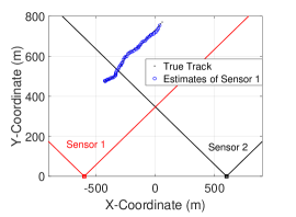
(a)

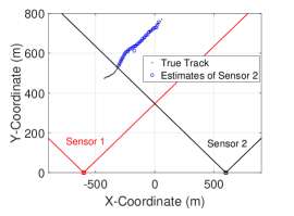
(b)

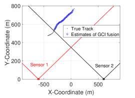
(c)

Figure 4: Posteriors outside FoV of Form I: (a) estimate of agent 1; (b) estimate of agent 2; (c) estimate after standard GCI fusion.

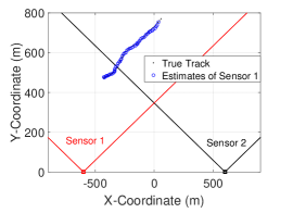
(a)

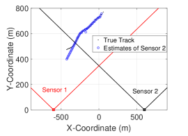
(b)

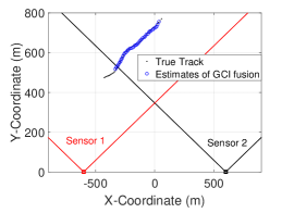
(c)

Figure 5: Posteriors outside FoV of Form II: (a) estimate of agent 1; (b) estimate of agent 2; (c) estimate after standard GCI fusion.

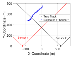
(a)

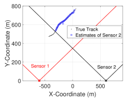
(b)

(c)

Figure 6: Posteriors outside FoV of Form III: (a) estimate of agent 1; (b) estimate of agent 2; (c) estimate after BIRD fusion.

Figs. 3-5 (a)-(c) respectively show the estimates of the two agents and the fusion results, for Forms I-III of posteriors outside FoVs. From Fig. 3 (a)-(c), it can be seen that adopting posteriors of Form I, GCI fusion can only preserve objects within the common FoV. Then, it can be seen from Fig. 4 (b), for agent 2, that when the object moves outside the FoV, the posterior actually becomes the prediction of the prior density, thus making estimation more and more inaccurate. Accordingly, the corresponding fusion result in Fig. 4 (c) becomes worse with time, since the discrepancy between posteriors of the two agents increases with time. Conversely, as shown in Fig. 5 (a)- (c), by adopting the uninformative density, BIRD fusion provides satisfactory performance for the whole track over the global FoV.

VI-B Performance assessment of BIRD fusion

This section aims to assess performance of the proposed BIRD fusion over distributed sensor networks, also making a comparison with centralized fusion and local (no fusion) tracking. The main adopted performance metric is the optimal sub-pattern assignment (OSPA) error [31]. A sensor network scenario with five sensors tracking six objects is considered, as depicted in Fig. 7 wherein objects appear and disappear at different times, during the $100\,[s]$ long simulations, as reported in Table I. The number of consensus steps for the distributed fusion is set to $L=3$.

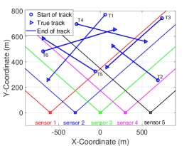
Figure 7: Simulation scenario: distributed sensor network with five sensors tracking six objects.

TABLE I: object birth and death times in the considered scenario.

object Birth Death object Birth Death T1 0 s 58 s T4 15 s 70 s T2 0 s 50 s T5 33 s 85 s T3 15 s 70 s T6 43 s 100 s

The five sensor nodes of the considered network can work in the following three modes:

1. (stand-alone mode) they just perform local filtering without any information exchange;

2. (distributed mode) they form a distributed network exchanging information and performing consensus-based fusion with neighbours;

3. (centralized mode) they form a centralized network sending posteriors to a fusion center which, in turn, feeds back the fused density to the sensor nodes.

Fig. 8 (a)-(c) shows the respective outputs of a single sensor (sensor 5) in M1, M2 and M3 modes for a single Monte Carlo run; similar bahaviours have been found for the other sensor nodes. Hence, the proposed fusion performs accurately and consistently in each node for the entire surveillance region, in the sense that each node maintains locking on all tracks and correctly estimates object positions in both distributed and centralized cases (modes M2 and M3). On the other hand, individual sensors working independently (mode M1) perform considerably worse in that each node is only able to track objects in its own FoV. In fact, whenever an object moves outside a node FoV, the node itself loses the object track very quickly as it cannot receive observations of it outside the FoV so that such track turns out to be terminated soon.

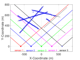
(a)

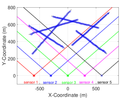
(b)

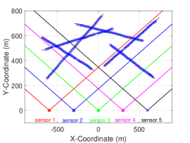
(b)

Figure 8: Single-run object tracks: (a) sensor 1 in mode M1; (b) sensor 1 in mode M2 (with 3 consensus steps); (c) centralized fusion (M3).

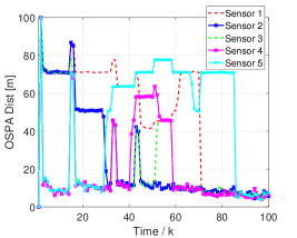
(a)

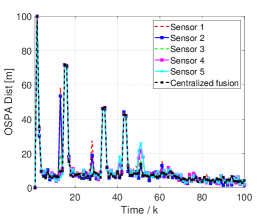
(b)

Figure 9: OSPA errors (averaged over $100$ Monte Carlo trials) at sensors $1-5$: (a) in mode M1; (b) in modes M2 (with 3 consensus steps) and M3 (centralized fusion).

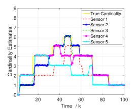
(a)

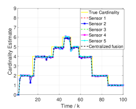
(b)

Figure 10: Cardinality estimates (averaged over $100$ Monte Carlo trials) at sensors $1-5$ (a) in mode M1; (b) in modes M2 (with 3 consensus steps) and M3 (centralized fusion)

Figs. 9 and 10 show the average (over $100$ Monte Carlo runs) OSPA errors and cardinality estimates of sensors 1-5 in M1, M2 and M3 modes. It can be observed that the five sensors working in M2 mode almost achieve the same performance in terms of OSPA error, approaching to the performance of the centralized case (M3) and can cope well with the situation that objects leave the sensor FoV. Conversely, there are remarkable performance differences among the five sensors working in M1 mode due to their different FoVs. Specifically, whenever an object moves outside a sensor FoV, performance of the latter in M1 mode is highly deteriorated (increased OSPA and cardinality errors). Notice that the Monte Carlo results of Figs. 9 and 10 are consistent with the single run results of Fig. 8. Further, it can be seen that when the performance of tracking/fusion algorithms (in mode M2) reaches a steady-state level, the OSPA error for each sensor node in the cooperative (M2 and M3) modes is significantly lower than in the stand-alone (M1) mode. Figs. 10 (a) and (b) present the cardinality estimates at sensors 1-5 under modes M1 and M2-M3, respectively. It is shown that cardinality estimates given by the sensors working in M2-M3 modes are more accurate than in M1 mode.

VII Conclusion

This paper addresses the problem of information fusion for multi-view multi-agent surveillance systems. To counteract the limitation of standard GCI fusion, we present a novel principled fusion rule, called Bayesian-operator InvaRiance on Difference-sets (BIRD). The proposed BIRD fusion provides a general and principled framework to combine the redundant information within the common FoV, and merge the complementary information within the exclusive FoVs, leading to a coverage of the global FoV. In particular, the proposed BIRD fusion can be performed on both a centralized and a distributed peer-to-peer sensor network. Simulation experiments on realistic multi-object tracking scenarios demonstrate effectiveness of the proposed solution.

References

- [1] G. Battistelli, L. Chisci, C. Fantacci, A. Farina, and A. Graziano, “Consensus CPHD filter for distributed multitarget tracking.” IEEE J. Sel. Topics Signal Process., vol. 7, no. 3, pp. 508–520, 2013.
- [2] C.-Y. Chong, S. Mori, and K.-C. Chang, “Distributed multitarget multisensor tracking,” Multitarget-multisensor tracking: Advanced applications, vol. 1, pp. 247–295, 1990.
- [3] R. P. Mahler, “Optimal/robust distributed data fusion: a unified approach,” in Proc. SPIE Defense and Security Symp., 2000, pp. 128–138.
- [4] M. Hurley, “An information-theoretic justification for covariance intersection and its generalization,” in Proc. IEEE Int. Fusion Conf., July 2002, pp. 7–11.
- [5] S. J. Julier, T. Bailey, and J. K. Uhlmann, “Using exponential mixture models for suboptimal distributed data fusion,” in Proc. IEEE Nonlinear Statist. Signal Process. Workshop (NSSPW’6), Cambridge, U. K., 2006, pp. 160–163.
- [6] D. E. Clark, S. J. Julier, R. Mahler, and B. Ristic, “Robust multi-object sensor fusion with unknown correlations,” in Sens. Signal Process. Defence (SSPD’10), Sep. 2010, pp. 1–5.
- [7] G. Battistelli, L. Chisci, C. Fantacci, A. Farina, and R. Mahler, “Distributed fusion of multitarget densities and consensus PHD/CPHD filters,” in Proc. SPIE Defense, Security and Sensing, vol. 9474, Baltimore, MD, 2015.
- [8] B. L. Wang, W. Yi, R. Hoseinnezhad, S. Q. Li, L. J. Kong, and X. B. Yang, “Distributed fusion with multi-Bernoulli filter based on generalized covariance intersection,” IEEE Trans. Signal Process., vol. 65, no. 1, pp. 242–255, Jan. 2017.
- [9] C. Fantacci, B.-N. Vo, B.-T. Vo, G. Battistelli, and L. Chisci, “Robust fusion for multisensor multiobject tracking,” IEEE Signal Processing Letters, vol. 25, no. 5, pp. 640-644, 2015.
- [10] S. Q. Li, W. Yi, R. Hoseinnezhad, G. Battistelli, B. L. Wang, and L. J. Kong, “Robust distributed fusion with labeled random finite sets,” IEEE Trans. on Signal Process., vol. 66, no. 2, pp. 278–293, Jan. 2018.
- [11] L. Gao and G. Battistelli and L. Chisci, “Random-finite-set-based distributed multi-robot SLAM,” IEEE Transactions on Robotics, vol. 36, No. 6, pp. 1758-1777, 2020.
- [12] S. Li, G. Battistelli, L. Chisci, W. Yi, B. Wang, and L. Kong, “Multi-sensor multi-object tracking with different fields-of-view using the LMB filter,” in 21st International Conference on Information Fusion (FUSION), 2018.
- [13] G. Li, G. Battistelli, W. Yi, and L. Kong, “Distributed multi-sensor multi-view fusion based on generalized covariance intersection,” Signal Processing, vol. 166, pp. 107–246, Jan. 2020.
- [14] X. Wang, A. K. Gostar, T. Rathnayake, and B. Xu, A. B. Hadiashar and R. Hoseinnezhad, “Centralized multiple-view sensor fusion using labeled multi-Bernoulli filters,” Signal Processing, vol. 150, pp. 75–84, Sep. 2018.
- [15] W. Yi, G. Li, G. Battistelli, “Distributed multi-sensor fusion of PHD filters with different sensor fields of view,” IEEE Trans. on Signal Process., vol. 68, pp. 5204–5218, Oct.. 2020.
- [16] K. Gostar, T. Rathnayake, R. Tennakoon, A. B. Hadiashar, G. Battistelli, L. Chisci and R. Hoseinnezhad, “Centralized cooperative censor fusion for dynamic sensor network with limited field-of-view via labeled multi-Bernoulli filter,” IEEE Trans. on Signal Process., vol. 69, pp. 878–891, Feb. 2021.
- [17] K. Da, T. Li, Y. Zhu and Q. Fu, “Gaussian mixture particle Jump-Markov-CPHD fusion for multitarget tracking using sensors with limited views,” IEEE Trans. on Signal Process., vol. 6, pp. 605–616, Aug. 2020.
- [18] A. K. Gostar, T. Rathnayake, R. Tennakoon, A. Bab-Hadiashar, G. Battistelli, L. Chisci, and R. Hoseinnezhad, “Cooperative sensor fusion in centralized sensor networks using Cauchy–Schwarz divergence,” Signal Process., vol. 167, pp. 107–278, Feb. 2020.
- [19] L. Gao, G. Battistelli, and L. Chisci, “Multiobject fusion with minimum information loss,” IEEE Signal Processing Letters, vol. 27, pp. 201-205, 2020.
- [20] T. Li and F. Hlawatsch, “A distributed particle-PHD filter using arithmetic-average fusion of Gaussian mixture parameters,” Information Fusion, 2021.
- [21] R. Mahler, Statistical multisource-multitarget information fusion. Norwood, MA, USA: Artech House, 2007.
- [22] J. K. Uhlmann, “Dynamic map building and localization for autonomous vehicles,” Unpublished doctoral dissertation, Oxford University, vol. 36, 1995.
- [23] T. Heskes, “Selecting weighting factors in logarithmic opinion pools,” in Advances in Neural Information Processing Systems, Cambridge, MA, USA: MIT Press, 1998, pp. 266–272.
- [24] H. Jeffreys, Theory of probablity. Oxford University Press, 1961.
- [25] E. T. Jaynes, “Prior probabilities,” IEEE Trans. on Systems Science and Cybernetics, vol. 4, no. 3, Sep. 1968.
- [26] J. K. Uhlmann, “Covariance consistency methods for fault-tolerant distributed data fusion,” Information Fusion, vol. 4, pp. 201–215, 2003.
- [27] L. Xiao, S. Boyd, and S. Lall, “A scheme for robust distributed sensor fusion based on average consensus,” in Proc. 4th Int. Symposium on Information Processing in Sensor Networks, Los Angeles, USA, 2005, pp. 63–70.
- [28] L. D. Stone, R. L. Streit, T. L. Corwin, and K.L. Bell, “Bayesian multiple target tracking”, Norwood, MA, USA: Artech House, 2014.
- [29] B.-N. Vo and W.-K. Ma, “The Gaussian mixture probability hypothesis density filter,” IEEE Trans. Signal Process., vol. 54, no. 11, pp. 4091–4104, 2006.
- [30] S. Julier and J. Uhlmann, “Unscented filtering and nonlinear estimation,” Proceedings of the IEEE, vol. 92, no. 3, pp. 401–422, 2004.
- [31] D. Schuhmacher, B.-T. Vo, and B.-N. Vo, “A consistent metric for performance evaluation of multi-object filters,” IEEE Trans. Signal Process., vol. 56, no. 8, pp. 3447–3457, 2008.
- [32] M. Beard, B.-T. Vo, B.-V. Vo, and S. Arulampalam, “A partially uniform target birth model for Gaussian mixture PHD/CPHD filtering,” IEEE Trans. Aerosp. Electron. Syst., vol. 49, no. 4, pp. 2835–2844, 2013.
- [33] J. Houssineau and D. Laneuville, “PHD filter with diffuse spatial prior on the birth process with applications to GM-PHD filter,” in Proc. IEEE Int. Fusion Conf., Jul. 2010.