Review on phase transformations, fracture, chemical reactions, and other structural changes in inelastic materials***Extended version of paper: Levitas V.I. Phase transformations, fracture, and other structural changes in inelastic materials. International Journal of Plasticity, 2021, Vol. 140, 102914, 51 pp., invited review. DOI 10.1016/j.ijplas.2020.102914
Abstract
Review of selected fundamental topics on the interaction between phase transformations, fracture, and other structural changes in inelastic materials is presented. It mostly focuses on the concepts developed in the author’s group over last three decades and numerous papers that affected us. It includes a general thermodynamic and kinetic theories with sharp interfaces and within phase field approach. Numerous analytical (even at large strains) and numerical solutions illustrate the main features of the developed theories and their application to the real phenomena. Coherent, semicoherent, and noncoherent interfaces, as well as interfaces with decohesion and with intermediate liquid (disordered) phase are discussed. Importance of the surface- and scale-induced phenomena on interaction between phase transformation with fracture and dislocations as well as inheritance of dislocations and plastic strains is demonstrated. Some nontrivial phenomena, like solid-solid phase transformations via intermediate (virtual) melt, virtual melting as a new mechanism of plastic deformation and stress relaxation under high strain rate loading, and phase transformations and chemical reactions induced by plastic shear under high pressure are discussed and modeled.
Notations
SCs Structural changes
PTs phase transitions
TRIP transformation-induced plasticity
CRs chemical reactions
RIP reaction-induced plasticity
SMA shape memory alloys
PFA phase field approach
DAC diamond anvil cell
RDAC rotational diamond anvil cell
G graphite
D diamond
FEM finite element method
IM intermediate melt(ing)
VM virtual melt(ing)
MD molecular dynamics
HPP high-pressure phase
, , and austenite, martensite, and martensitic variant
Direct tensor notations are used throughout this paper. Vectors and
tensors are denoted in boldface type; and are the contraction of tensors
over one and two nearest indices. Superscripts and denote
inverse operation and transposition, respectively, means equals per definition, subscript
designates symmetrization of the tensors, the indices 1 and
2 indicate the values before and after the SC.
Subscripts , , and designate elastic, transformational, and plastic deformations or deformation gradients.
1 Introduction
Solid-solid phase transformations (PTs) are broadly studied in physical, material, and mechanical experiments. They are utilized in modern technologies (e.g., thermal and thermomechanical treatments of metals, shape memory and elastocaloric applications, and high-pressure technologies) and broadly spread in nature, e.g., in geophysical processes. In most cases, PTs are accompanied by plastic deformations; in some cases, they are caused by plastic deformations (plastic strain induced PTs). Googling ”phase transformation and plasticity” returns 13,600,000 results. It is clear that any attempt of review on this topic will miss many important aspects. We will focus on topics and papers, which we worked on for several decades, and on works which have affected us. There are multiple reviews related to the interaction between PT and plasticity (e.g., [372, 144, 317] on material aspects, [65, 407] on shape memory alloys, on the continuum mechanical aspects [228, 110, 246], transformation-induced plasticity (TRIP) [113, 348], PTs and structural changes (SCs) under high-pressure torsion [41, 42, 474, 476, 88, 89, 28, 434, 477, 435, 436, 87, 336, 417, 252], and mechanochemistry [203, 287]), and we will avoid overlapping.
One of the broad topics of this review is the development of general thermodynamic and kinetic approaches to SCs in inelastic materials within a sharp interface approach. SCs under consideration include various PTs (martensitic, reconstructive, melting, sublimation, and others), twinning, chemical reactions (CRs), and fracture (crack and void nucleation and growth). A well-known formalism was developed for the description of the evolution and interaction of various defects or singularities in elastic materials [94, 95, 96, 97, 389, 390, 55, 56]. They include phase interfaces, grain and twin boundaries, crack tips and voids, and point and linear defects, participating in such structural changes as PTs, grain evolution, damage, and plastic deformation. For each of these defects, the rate of energy release or dissipation rate can be written as , where is the defect velocity relative to the material and is the generalized material/driving force acting on the defect [94, 95, 97]. The formula for is derived, where is the Eshelby energy-momentum tensor, is an arbitrary surface with the unit normal surrounding the defect and separating it from other defects or the actual surface defect (e.g., phase interface or grain boundary). This concept was extended for or rediscovered in various specific fields. For example, in fracture mechanics, a driving force was introduced as a path-independent -integral [389, 390] or -integral [55, 56]; see also [129, 130, 193] for PTs and [334, 335] for Eshelbian mechanics. Since, for elastic materials, dissipation occurs due to the motion of defects only, adding to the integral over the volume without evolving defects does not change the dissipation rate and –this explains the independence of of the surface (or integration path).
For inelastic materials, the dissipation due to plastic deformation and change in internal variables contributes to the total dissipation rate in the volume surrounded by surface and depends on the choice of surface . Even for the volume tending to zero, i.e., when it includes the defect only, inelastic dissipation in the singular point or surface still takes place (e.g., at the crack tip or moving interface). It is not easy to split the dissipation due to the defect evolution itself and plastic deformation. That is why it was accepted in works on fracture mechanics [389, 205, 11, 204] that the strict thermodynamic criterion for ductile fracture is not developed and other approaches like energy flow in an infinitesimal or finite-sized process zone [389, 56, 166, 11], total dissipation rate [430, 205], plastic work [210], critical plastic strain [337, 389], critical crack tip opening displacements [150], -integral (or - integral) without separation of plastic dissipation [55, 56], and others are used. A similar situation took place in PT theory, see Section 6.
For elastic materials, the conditions for both the appearance of a defect (”nucleation”) and its equilibrium are described by the principle of the minimum of Gibbs free energy. That is why they coincide. Thus, from a thermodynamic (but not a kinetic) viewpoint, it is not necessary to treat a nucleation process separately; it is sufficient to insert a nucleus and study its equilibrium using the local condition, e.g., for an interface or crack tip. However, for inelastic materials, defect nucleation and equilibrium conditions are different. Thus, a defect nucleation problem within inelastic materials has to be formulated and solved. Defect nucleation and evolution in inelastic materials cannot be described by the principle of the minimum of Gibbs energy or with the help of an energy-momentum tensor only. Thus, the new driving force and extremum principle for the determination of all unknown parameters (e.g., position, shape, orientation, and internal structure of the nucleus of a product phase) are required. In contrast to elastic materials, since the constitutive behavior of inelastic materials is history dependent, analysis of the entire transformation-deformation process in the transforming region is required.
Another broad topic of this review is the development of phase field approaches (PFAs) to different SCs in inelastic materials, see e.g., [9, 189, 413, 449, 447, 452, 146, 195, 394, 253, 272, 271, 182, 306, 177]. PFA is based on the concept of the order parameters that describe instabilities of the crystal lattice during PT, twinning, dislocation nucleation, and fracture, as well the evolution of phase and dislocational structures in a continuous way by solving Ginzburg-Landau evolution equations for the order parameters. Typical solutions for these equations are propagating finite-width phase and twin interfaces, crack surfaces, and dislocation core regions that describe the evolution of complex microstructures. Thermodynamic potential has as many minima in the space of the order parameters as many phases and structural states system possesses. These minima are separated by energy barriers. Besides, the thermodynamic potential depends on the gradients of the order parameters, which are concentrated at the finite-width phase and twin interfaces, crack surfaces, and dislocation cores; this reproduces the interface, surface, and dislocation core energies.
The sharp-interface approach gives specific expressions for the thermodynamic driving forces for the nucleation and evolution of defects. It is convenient for solving problems with relatively simple geometries of interfaces and defects, and allows analytical solutions for some problems. The PFA includes additional information about the stability and instability of phases and different states. It allows for studying the evolution of arbitrary complex geometries of interfaces and defects, without any computational cost on tracking interfaces. Thus, both approaches have their advantages and disadvantages, and they supplement each other. Both will be reviewed in the current paper.
This review is organized as follows. In Section 2, short background information on martensitic PTs in inelastic materials is presented, including some examples of interactions between PTs and plasticity. In Section 3, some universal kinematic and balance relationships for a coherent interface in an arbitrary medium are presented. Thermodynamic and kinetic descriptions of PTs in elastic materials are discussed in Section 4. Athermal resistance to interface propagation and its relationship to the yield strength are introduced in Section 5. General sharp-interface thermodynamic and kinetic theories for SCs in inelastic materials are presented in Section 6. They include the driving forces and thermodynamic criteria for nucleation and interface propagation, and the extremum principle for determination of all unknown parameters that substitutes the minimum Gibbs energy principle for elastic materials. Three types of kinetics are described: athermal kinetics, thermally-activated kinetics, and ”macroscale” thermally-activated kinetics. In addition, the global SC criterion based on stability analyses is introduced. Peculiarities of the finite strain approaches are summarized in Section 7. All equations from last two Sections are summarized in ten boxes. Sections 8, 9, and 10 present some analytical solutions based on the developed theory, which illustrate the main points of the theory as well as their application to some real problems. They include SC in a sphere (with application to PT from graphite to diamond), PTs and CRs in a shear band (with application to transformation- and reaction-induced plasticity (TRIP and RIP)), consideration of a propagating interphase, as well as PT in an ellipsoidal inclusion. Various aspects of the nucleation and growth of a martensitic region with coherent, semicoherent, and incoherent interfaces, as well as interfaces with decohesion are analyzed with the finite element method (FEM) in Section 11. Both the sharp-interface theory and PFA are utilized. Sections 12 and 13 are devoted to recently revealed nontraditional mechanisms of PTs in solids via intermediate (virtual) melt and mechanism of plastic deformation and stress relaxation under high strain rate loading via virtual melting, both much below the melting temperature, when melting is not expected. Strain-induced martensite nucleation at the shear-band intersection was studied with FEM in Section 14. The importance of the application of the global criterion for SCs based on stability analysis was demonstrated. The appearance and growth of a martensitic plate in an elastoplastic material for temperature-induced PT was analyzed with FEM in Section 15. The effect of the inheritance of plastic strain on a large change in the plate’s shape and on the arrest of plate growth (i.e., morphological transition from the plate to lath martensite) is demonstrated. Nanoscale and microscale PFAs to the interaction between dislocation plasticity and PTs are described in Section 16. In Section 17, a multiscale theory of strain-induced SCs under high pressure is presented for the interpretation of various phenomena during compression and shear of materials in a rotational diamond anvil cell. Scale transitions and phenomenological theories for the interaction between PT and plasticity are analyzed in Section 18. Fracture and the interaction between fracture and PT in inelastic materials are described within both the sharp-interface theory and PFA in Section 19. Concluding remarks are presented in Section 20.
2 Martensitic transformations in inelastic materials: some background information
We will focus on displacive PTs, which are dominated by the deformation of a unit crystal cell of the parent phase into a unit cell of the product phase that is described by transformation deformation gradient , where is the orthogonal rotation tensor, is the transformational right stretch (Bain) tensor, and is the transformation strain tensor. Note that produces mapping of the stress-free crystal lattice of the parent phase into that for the product phase at a fixed temperature. Usually, the higher symmetry and higher temperature phase is called the austenite, and the lower symmetry and lower temperature phase is called the martensite.
Displacive PTs include martensitic PTs during which atoms do not change their neighbors and reconstructive PTs in the opposite case. In addition to , displacive PT involves intra-cell displacements or shuffles. The diffusion of species does not occur during martensitic PTs.
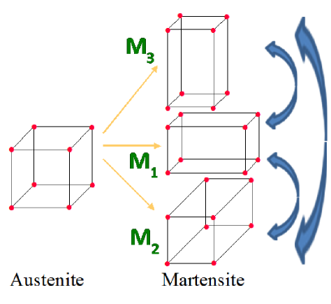
Due to the symmetry of crystal lattice, there is a finite number (e.g., 3 for the cubic to tetragonal PT and 12 for the cubic to monoclinic PT) of crystallographically equivalent martensitic variants (Fig. 1). Lists of the transformational right stretch tensors for various PTs and for all martensitic variants are presented, e.g., in [26, 382]. The transformation strain can be quite large. For example, for cubic to tetragonal PT from Si I to Si II [464] and cubic to monoclinic PT from rhombohedral graphite to hexagonal diamond [44] tensors are
| (7) |
The components of , , for cubic to tetragonal PT from phase I to II in Ge and GaSb, as well as for PT in Sn, are in the range and [327]. For the layer-puckering mechanism [43] for PT from cubic diamond and boron nitride to rhombohedral graphite and BN, and . Transformation strain is generally much larger than the maximum elastic strain, which varies from for steels to for NiTi and CuZnAl shape memory alloys.
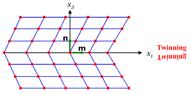
Most of the martensitic variants are in twin relationship to each other. Twinning is a simple shear of one part of the crystal lattice with respect to another up to a position in which it represents a mirror reflection of the initial lattice (Fig. 2). Thus, twinning is described by the transformation deformation gradient , where is the twinning shear strain that occurs in the direction in the plane with the normal , which is called the twinning plane. Generally, twinning is a mechanism of plastic deformation in crystalline materials whereby jump-like shear deformation of the crystal lattice occurs. It both competes with and supplements dislocation plasticity. For the body-centered cubic (bcc) lattices (for example, in Mo, Na, and Cr) and the face-centered cubic (fcc) metals (for example, in Al, Cu, and Co), the magnitude of the transformation shear is very large. For the hexagonal close-packed (hcp) lattice in Mg and in Zr . For the body-centered tetragonal lattice in NiAl . Various aspects of twinning can be found in the books [453, 26, 202, 382]. An example of the constitutive equations for twinning can be found in [339] and references herein. As a mechanism of plastic deformation, in which twinning competes with dislocations, twinning usually occurs at a lower temperature, higher strain rates, and smaller grain size than the dislocation plasticity. Such competition also takes place during PTs. Since a single martensitic variant is generally not compatible with austenite and generates large internal stresses, these stresses relax either by twinning (for example, in shape memory alloys and some steels) or by plastic slip (for example, in steels), or both, producing an invariant plane strain variant with averaged transformation deformation gradient , where is the invariant plane shear strain along the direction in the invariant (or habit) plane with the normal , and is the normal to habit plane strain. Typical values of are around zero for NiTi and CuZnAl shape memory alloys, 0.02 to 0.05 for steels, and 0.2 for PT in plutonium; typical values of are 0.1-0.2 for shape memory alloys, 0.2 for steels, and 0.27 for PT in plutonium.
Usually, three types of PTs are distinguished: temperature-induced, stress-induced, and strain-induced. Temperature-induced PTs occur without external stresses, and nucleation starts at pre-existing defects (e.g., dislocations, point defects, grain and subgrain boundaries, stacking faults, and twins). Stress-induced (or assisted) PTs take place under external stresses below the macroscopic yield strength by nucleation at the same pre-existing defects as temperature-induced PTs. Strain-induced PTs occur during plastic deformation by nucleation at new defects generated by plastic flow [367, 369, 370, 372].
Formally, we define any type of the SCs enumerated above (PT, CRs, twinning, and fracture) as a thermomechanical deformation process of the growth of transformation strain from its initial value in the parent phase to the final value in the product phase, which is accompanied by a change in all the thermomechanical properties (elastic moduli of an arbitrary rank, thermal expansion tensor, specific heat, etc.).
Below we outline some examples of interaction between SCs and inelasticity, which are interrelated.
1. PTs and other SCs, possessing a transformation strain, are processes of an inelastic deformation in materials. For some materials and applications, for which traditional (dislocation or twinning) plasticity is not desirable, like shape memory alloys (SMA), strong ceramics, and semiconductors (like Si and Ge), PT is the main mechanism of inelasticity. For all other cases, transformation strain supplements dislocation plasticity and twinning.
2. Microplastic straining, which occurs in SMA during cyclic loading, accumulates and leads to defect generation, damage, and degradation of transformational properties (e.g., reduces recoverable strain and increases stress hysteresis and energy losses).
3. Slip and twinning in martensite (a combination of two martensitic variants) are mechanisms for lattice-invariant shear. Along with the transformation (Bain) strain and crystal lattice rotation, they produce an invariant plane strain variant [453] between austenite and martensite. This process is driven by the reduction of the energy of internal stresses; it promotes nucleation and growth.
4. Transformation strain in the transforming regions generates internal stresses, which in most cases exceed the yield strength and produce accommodational plastic strains within and outside of the transforming regions. Reduction of the internal stresses increases the thermodynamic driving force for nucleation. However, stress redistribution caused by plastic deformation near the growing product phase reduces the thermodynamic driving force for interface propagation. In elastic materials, the martensitic region is arrested by a strong obstacle (e.g., grain, subgrain, or twin boundaries, or another martensitic region), producing plate martensite morphology. Plasticity stops the growth of martensitic units inside the grain before reaching an obstacle, leading to a morphological transition to the lath martensite. Numerous analytical and numerical results illustrating the above statements are presented in the following Sections.
5. Plastic deformation generates a group of defects (e.g., dislocation walls or pileups), and corresponding stress concentrators produce nucleation sites for PT. At the same time, chaotic defect structures like dislocation forests resist the interface propagation. Preliminary plastic deformation generally suppresses martensitic PTs.
6. Plastic flow that occurs during PT causes strain-induced PT, which proceeds by nucleation at defects generated during plastic flow, e.g., at a dislocation pileup or slip-band intersections. While for stress-induced PTs, the PT stress grows linearly with the temperature increase, for strain-induced PTs, the PT stress reduces with the temperature rise due to the reducing yield strength but grows with increasing plastic strain due to strain hardening.
7. Internal stresses caused by transformation strain in superposition with external stresses, which may be well below the yield strength, cause plastic flow. This phenomenon is called TRIP for PTs [113, 348, 367, 374, 463] or RIP for CRs [278, 279]. They serve as a relaxation mechanism for internal stresses and as an additional mechanism of inelastic deformation. For cyclic direct-reverse PT under the external stress, below the yield strength, TRIP is accumulated in each cycle and may exceed hundreds of percent.
8. The phase interface, similar to a twin interface, can be presented as an array of partial dislocations [372]. In such a representation, PT consists of the nucleation and motion of these dislocations, like dislocation plasticity.
9. Some PTs, in addition to transformation strain, involve shuffles (intracell atomic motion) produced by the motion of partial dislocations, e.g., for bcc-fcc and fcc-hcp PTs [383].
10. The strong promoting effect of the plastic shear under high pressure on PTs and CRs will be discussed in Section 17.
Knowledge of the influence of plastic strain and applied and local stress fields on SCs is very important for the understanding, simulation, and improvement of the technical processes, as well as for the development of new technologies and materials. Examples include heat and thermomechanical treatment of materials; increasing toughness utilizing TRIP; severe plastic deformation technologies, including high pressure torsion and ball milling, friction, wear, surface treatment (polishing and cutting); as well as the interpretation of earthquakes.
3 Some universal relationships for a coherent interface
Let the motion of the homogeneously deformed small vicinity of a material point be described by the function , where and are the positions vectors in the actual and reference configurations and is time. The deformation gradient is . We will not focus on the multivariant structure of martensite here, and will instead consider a two-phase material.
For a coherent interface, when a jump in displacement across an interface is absent, but the particle velocity vector and the deformation gradient have a jump, the Hadamard compatibility condition is valid in the reference configuration [426]
| (8) |
where is the unit normal to the interface in , is the interface velocity, and is the jump of parameters across the interface. The conservation of mass at the interface is expressed as
| (9) |
where is the mass density. Neglecting inertia, the traction continuity condition at the interface is
| (10) |
where is the non-symmetric first Piola-Kirchhoff stress tensor.
4 Phase transformations in elastic materials
As an initial step and for comparison, we will describe an approach to phase transformations in elastic materials in the reference configuration. Let us consider a volume of a two-phase material with the prescribed traction at the part of the boundary and displacement at the rest of the boundary ; . The dissipation at the interface between phases is neglected. The problem is to find a two-phase configuration in thermodynamic equilibrium. For isothermal processes the total dissipation increment due to variation of the position of the interface is
| (11) |
where is the temperature, the Helmholtz free energy per unit mass, and is the interface energy per unit reference area. Note that if , it does not produce surface stresses and does not change the traction continuity condition (10) (in contrast to the case when the surface energy per unit deformed area or when depends on strain). If is fixed, then Eq. (11) can be presented in the form
| (12) |
where is the Gibbs energy of the system body+loading. Thus, phase equilibrium for an elastic material, i.e., the geometry of the interface, is determined by the stationary value of the Gibbs energy. If the Gibbs energy has a local minimum, phase equilibrium is stable; otherwise, it is unstable. If a stable interface does not exist under the prescribed boundary conditions, then only the single-phase solution is stable.
Let us consider each phase separately, without interfaces. The Gibbs energy can then be introduced for the parent phase (subscript 1) and product phase (subscript 2):
| (13) |
| (14) |
Here, is the local Gibbs energy per unit mass of each phase, expressed in terms of with the help of the elasticity rule; the divergence theorem was used to transform surface integral into a volume integral, and the equilibrium equation has been utilized. Since analytical inversion of the elasticity rule is in most cases impossible in practice, one can keep the argument in , and should numerically correspond to the given .
For a given traction (or, for homogeneous stress, a given stress tensor ) and temperature, the phase with smaller Gibbs energy is called the stable phase, and the other is called the metastable phase. The transition from a metastable to stable phase is accompanied by the reduction in Gibbs energy and a positive dissipation increment (see Eq. (12)), i.e., it is thermodynamically possible. However, it does not mean that this transition will occur because there is usually an energy barrier between phases. When an energy barrier disappears due to change in traction or temperature, the metastable phase becomes unstable and barrierless PT occurs. PT from the phase with the lower Gibbs energy to the higher energy is thermodynamically impossible. Phases with equal Gibbs energy are considered to be in thermodynamic equilibrium. This definition has a physical sense for hydrostatic media, liquids, and gases under prescribed pressure, because (with neglected surface tension (stresses)) the pressure is the same in both phases. For solids, phase equilibrium should be considered across an interface and not the entire stress tensor; only traction remains the same across an interface (Eq. (12)). Of course, phase equilibrium conditions are different for different interface orientations. Still, in high-pressure research, phase equilibrium is defined by equality of the Gibbs energies of phases under prescribed pressure.
It is also clear that the definition of the Gibbs energy and related definitions depend on the chosen stress measure and boundary conditions, i.e., which components of stresses are fixed at the boundary. Integrating Eq. (12) over the time for the appearance of a nucleus of phase 2 in a finite volume , we obtain
| (15) |
i.e., the total dissipation increment is equal to the negative difference between the Gibbs energy of the final and initial states, and represents the global thermodynamic driving force for the PT. Eq. (15) will be used as the main hint and limiting case for checking when we will develop SC theory for inelastic materials.
Let us transform Eq. (11) for the neglected interface energy using the divergence theorem and the rule of differentiation for the volume integral, both for a volume with moving surfaces with discontinuous velocity or a deformation gradient:
| (16) |
| (17) |
where Eqs. (8) and (10) were used. Substituting Eqs. (16) and (17) into Eq. (11), we obtain
| (18) |
Due to the independence of both integrals and arbitrariness of and , both integrands in Eq. (18) are equal to zero. The first integrand results in the nonlinear elasticity rule for points of the volume. The second results in the phase equilibrium condition at the interface
| (19) |
where is the thermodynamic driving force for the interface motion. Eq. (8) was utilized in the derivations. The expression for in Eq. (19) is also called the Eshelby driving force for the interface propagation per the celebrated work [93], where it was derived. The chemical potential tensor in the reference configuration was introduced in [129, 130], where various aspects of phase equilibrium and different chemical potentials are discussed (see also [206, 193] and references). For geometrically linear approximation, , where and are the small symmetric strain and antisymmetric spin tensors, respectively, is the symmetric stress tensor and Eq. (19) simplifies
| (20) |
When isotropic surface energy is taken into account, Eq. (19) generalizes to
| (21) |
where is the mean interface curvature.
The following static problem formulations are usual for PTs in elastic materials:
1. For the prescribed boundary conditions, find a two-phase solution within a body. Solutions (possibly multiple) correspond to the stationary value of the Gibbs energy (Eq. (12)) or local thermodynamic equilibrium condition Eq. (21) for each point of a phase interface.
2. For the neglected interface energy for the problem in item 1, one can find external tractions and displacements at which the two-phase equilibrium becomes possible for the first time. This is the initiation of the PT. Examples include the minimum pressure for PT from a low-pressure to high-pressure phase or the maximum pressure for PT from a high-pressure to low-pressure phase. The critical conditions for PT initiation can be found from the solution for a small inclusion of the product phase in item 1 when the characteristic size of the inclusion tends to be zero while keeping a shape that minimizes the Gibbs energy. This zero size explains why surface energy should be neglected.
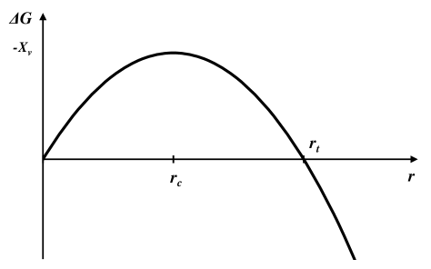
3. When surface energy is included, an unstable stationary solution called the critical nucleus plays an important role. It corresponds to the minimax of the Gibbs energy, the minimum with respect to the shape (and all internal parameters, like a twinned structure, if included) and the maximum with respect to the size or volume of the nucleus (Fig. 3). The energy increment for the critical nucleus, is the difference between the energy of the critical nucleus and the energy of the parent phase, which can be any phase the material is initially in. The energy of the critical nucleus is higher than the energy of the parent phase and its appearance causes a negative dissipation increment. Since the appearance of the critical nucleus is not thermodynamically favorable and requires fluctuations, it cannot be described by traditional continuum thermodynamics based on two thermodynamics laws. While it was well-known in material literature that the energy grows during the appearance of a critical nucleus (i.e., dissipation increment is negative), this statement caused a psychological problem for the continuum mechanics community, which required some tutorial explanations in [250]. Earlier, in the treatment of nucleation in elastic materials in [319], it was specified that nucleation produces, rather than dissipates, energy and that the subcritical nuclei cannot grow due to the restriction produced by dissipation inequality. In [243, 244], after stating that the appearance of the critical nucleus is accompanied by a negative dissipation increment, thereby requiring thermal fluctuations, the concept of the thermodynamically admissible nucleus was suggested. In particular, the nucleus of the radius in Fig. 3 corresponds to , i.e., it is thermodynamically admissible. However, such a treatment is not consistent with the existing textbook approaches on nucleation, and it does not explicitly determine the activation energy. This concept appears naturally within a phenomenological theory of the appearance of a finite region of a product phase without going into detail about complex nucleation-growth processes. The approach in [243, 244] illustrates that, in general, there is nothing unusual in the nucleation and that the second law is satisfied for the event, averaged over the size or the corresponding time interval. The problem arises because we are interested in the event that occurs during a shorter period of time, and it is not surprising that the second law of thermodynamics is not applicable for such a scale.
Indeed, continuum thermodynamics operates with parameters that are averaged over some time and volume, and any fluctuations are filtered out. As a result, the nucleation process is generally described by statistical theories (as seen in [197]), which we will not discuss here.
General ideas of the thermally activated kinetics can be found in classical nucleation theory [108, 429, 383]. The Arrhenius-type equation for the nucleation time in a sample with volume is
| (22) |
Based on the probability consideration, the pre-exponential factor is usually considered to be inversely proportional to the volume of the entire sample . The activation energy for thermally activated nucleation is equal to the energy of the critical nucleus . We write
| (23) |
The first maximum in Eq. (23) belongs to the definition of the critical nucleus. All minima are motivated as follows: the smaller the activation energy, the smaller the nucleation time. Consequently, a nucleus with the smallest activation energy should appear first. That is why in Eq. (23) activation energy is minimized with respect to all relevant parameters.
The traditional criterion for thermally activated nucleation is
| (24) |
which is determined from the condition that, for larger , the nucleation time exceeds any realistic time of observation for any choice of pre-exponential parameters in the Arrhenius-type kinetic equation [383, 313, 247, 246]. Here is the Boltzmann constant. While criterion (24) is from a material science textbook on PTs [383] and broadly used in the treatment of PTs by material scientists [383, 313], its application was limited in the continuum mechanics community [247, 246, 255, 256, 250, 257, 284]. Note that definition (23) includes an extremum principle for the determination of all unknown parameters of the nucleus.
Since the critical nucleus cannot appear thermodynamically, it should be introduced ”by hand” into the problem for continuum treatment. This allows the nucleus slightly larger than the critical one (supercritical nucleus) to grow in a thermodynamically consistent way. The nucleus slightly smaller than the critical one (subcritical nucleus) shrinks and disappears. In the phase-field approach, nucleation is modeled by including a stochastic term in the Ginzburg-Landau or Cahn-Hilliard equations, which satisfies the dissipation-fluctuation theorem (see, e.g., [188, 315, 446, 9]).
5 Athermal resistance to interface propagation
Athermal resistance for interface propagation is analogous to dry friction in classical mechanics: interface propagation occurs only if the driving force exceeds a rate-independent threshold . The athermal resistance is responsible for deviation of the actual SC stress or/and temperature from their thermodynamical equilibrium values, and consequently, for stress or/and temperature hysteresis during forward-reverse SC, and for energy dissipation, when interface velocity is small and viscous friction is negligible. It is observed for SCs both in elastic (e.g., in shape memory alloys) and elastoplastic materials. Inclusion of the athermal dissipation in the description of PT in elastic materials significantly and conceptually complicates the description of the transformation process, similar to the mechanics of the system with dry friction. Thus, the entire behavior becomes loading-path dependent and should be treated incrementally. The thermodynamic equilibrium does not correspond to the minimum of the Gibbs energy, and the principle of stationary Gibbs energy cannot be applied for searching a two-phase equilibrium microstructure. Such features are closer to those for PTs in elastoplastic materials. Extremum principle substituting the principle of the stationary Gibbs energy for SCs in elastic materials with athermal friction were obtained in [240] as a particular case of the corresponding principle for PTs in elastoplastic materials. Mathematic treatment of the problem for SCs in elastic materials with athermal interfacial resistance was initiated in [347].
There are several sources of athermal interfacial friction [125]:
-
1.
Peierls barrier, which appears due to the discrete periodic structure of the crystal lattice, similar to that for dislocations.
-
2.
Interaction of a moving interface with a long-range stress field of various defects, e.g., point defects (solute and impurity atoms, vacancies), dislocation forest, stacking faults, grain, subgrain, and twin boundaries, and precipitates.
-
3.
Emission of acoustic waves.
When SC is considered in a finite volume, an additional contribution to the athermal dissipation and SC hysteresis is related to a nucleation barrier. An athermal threshold is determined as a minimum value of the driving force at which SC occurs, i.e.,
| (25) |
where is a locally determined athermal threshold per unit mass and is an athermal threshold averaged over a nucleus per unit mass. If the volume is transformed by continuous interface propagation, then .
By definition, the athermal threshold cannot be overcome by thermal fluctuations. While the magnitude of can be different for direct and reverse SC and based on a variety of the mechanisms, is expected to be dependent on the entire deformation-SC process and the evolving material microstructure. However, a simple relationship
| (26) |
was suggested in [238, 240] based on the comparison of some high-pressure experiments summarized in [28] with the solution of the corresponding boundary-value problems. Here is the yield strength, which is the function of the temperature , plastic strain , and set of internal variables , is the proportionality factor, and is the volumetric transformation strain, which can be included in . The values for some PTs are determined in [238, 240]. Physically, the proportionality between and is caused by the fact that and characterize resistance to the dislocation and interface motion, respectively, through the same material microstructure consisting of various point, linear, planar, and bulk defects. For large plastic deformations, based on the regularity revealed in [236], and consequently reach their maximum and are independent of plastic strain and strain-history. Since experiments in [28] were performed in 1980-1983, utilization of modern diagnostic, like x-ray diffraction with synchrotron radiation, may change our understanding of the effect of plastic strain on the athermal threshold.
For SMAs, the stress hysteresis and dissipation are proportional to . Since both the stress hysteresis and linear depend on plastic strain, as seen in experiments in [157, 411, 412, 425], this also supports Eq. (26). A slightly different but close relationship between and the yield strength of an austenite for steel is suggested in [125, 126] and presented in Eq. (64).
6 Theory of structural changes in inelastic materials with an unstable intermediate state
For the description of SC in an elastic solid, the explicit equation for the thermodynamic driving force for the interface propagation and corresponding local thermodynamic equilibrium condition (Eqs. (19) and (21)) for each point of a phase interface are known. They correspond to the stationary value of the Gibbs energy (Eq. (12)). The activation energy for a critical nucleus Eq. (23) is also determined in terms of the Gibbs energy. Furthermore, each solution of the elastic problem (including cases where there are multiple solutions for given boundary conditions) is independent of the process and depends on the final boundary conditions.
For inelastic materials, such results are lacking. All processes in plasticity are loading-history dependent and accompanied by energy dissipation, even for infinitesimally slow processes. For this reason, a change in the Gibbs energy alone does not define the driving force, and the stationarity of the Gibbs energy does not determine the phase equilibrium or critical nucleus. A conceptually different thermodynamic approach was required to determine the thermodynamic driving force for nucleation and interface propagation, the definition of the critical nucleus, the expression for the activation energy for the critical nucleus, and the extremum principle for the determination of all unknown parameters of the nucleus. Eq. (15) will be utilized as the main hint for the formulation of the driving force for SC in inelastic materials: it should have a sense of the dissipation increment due to SC only for the appearance of a complete nucleus.
We will present our theory developed in [240, 243, 244] and [250, 257]. Initially [229, 232, 233, 238, 239], the nucleation condition was postulated in the form of the dissipation increment due to PT only (excluding plastic and other types of dissipation) reaching its experimentally determined value related to the athermal threshold. Later in [234, 235, 240, 243, 244], a local description of PTs was developed for better justification, which we will use here.
6.1 Definition of the structural changes without a stable intermediate state and local equations
For simplicity and transparency of the main ideas, we will start with the geometrically linear formulation. The main local equations describing SC are collected in Box 1.
Traditional additive kinematics (27) is utilized. It is convenient to introduce a scalar parameter describing SC: SC starts at and completes at . The parameter is an internal variable similar to a volume fraction of the product phase in the mixture theory or order parameter in the PFA. The parameter can be determined by Eq. (28) or a similar equation based on any other material property of the phases, such as elastic moduli or entropy. For the Helmholtz free energy, we assume Eq. (29), where is a set of internal variables describing plasticity, e.g., back stress or dislocation density. Traditional thermodynamic treatment results in the constitutive equations (30) for stress and entropy, the yield condition (33), and the evolution equations for plastic strain and internal variables (34). It is assumed that -dependence of all material properties is known, e.g., based on linear interpolation between properties of two phases, similar to the simplest mixture theory.
Note that in contrast to the PFA or mixture theory, we do not prescribe the local evolution equation for describing the SC. We assume that the SC process at each point of the transforming volume cannot be stopped in an intermediate stage. Consequently, the material in each material point can only be in either phase 1 or phase 2. Such SC is coined in [243, 244] as the SC without a stable local intermediate state, and the following definition is used.
The SC will be considered as a process of variation of the transformation deformation gradient and some or all thermomechanical properties in an infinitesimal or finite transforming volume from the initial to the final value. This process cannot be stopped at an intermediate state in any transforming point. Thermodynamic equilibrium for an intermediate value of the transformation deformation gradient or material properties is impossible.
Such a definition excludes from consideration the Landau-Ginzburg model (see Section 16.1), in which a smooth transition from phase 1 to phase 2 occurs due to a nonlocal term, and any intermediate state can be stable inside a diffuse interface of finite thickness. We will focus on the case with a sharp interface and local constitutive equations describing the deformation in each material point.
1. Additive decomposition of strain into elastic , plastic , and transformational parts
| (27) |
2. Internal time
| (28) |
3. Local constitutive equations
3.1. Helmholtz free energy per unit mass , elastic and thermal energies
| (29) |
3.2. Elasticity rule and entropy-temperature relationship
| (30) |
3.3. Dissipation rate per unit mass due to plastic flow and variation of the internal variable
| (31) |
3.4. Dissipative forces for plastic flow and variation of the internal variable
| (32) |
3.5. Yield condition
| (33) |
3.6. Evolution equations for plastic strain and internal variables
| (34) |
6.2 Thermodynamic driving forces for nucleation and interface propagation

Our goal here is to generalize the thermodynamic driving forces for nucleation and interface propagation derived for elastic materials (Eqs.(15) and (19)) for those in inelastic materials.
Problem Formulation. Let us consider some region of a material undergoing SCs under the prescribed boundary conditions in tractions and displacements at a boundary (Fig. 4). Nucleation of phase 2 will be considered as the SC that starts and completes in some region with the boundary during the nucleation time . In practice, we change the field of the parameter from 0 to 1 in the nucleus, homogeneously or heterogeneously, which introduces into the nucleus the transformation strain field and variation of all material properties from properties of phase 1 to properties of phase 2— all without changing the boundary conditions. This process represents the prescribed deformation process, for which the inelastic boundary value problem and heat conduction equation should be solved incrementally, producing fields , , , , and all other participating fields. Note that depending on the goal, we will use a different definition of a nucleus. In addition to the traditional critical nucleus, we will also consider the appearance of a macroscopic region that is formed during nucleation and growth processes. Having this information, one must answer the following four questions:
1. What is the thermodynamic driving force for the nucleation and phase interface propagation?
2. Is SC possible for the chosen boundary and initial conditions, i.e., what is the SC criterion?
3. How do we determine all the unknown parameters of a nucleus and the transformation process in it, i.e. the position, volume, shape, and orientation of a nucleus, its internal structure (i.e., actual field ? All unknown parameters will be collectively designated as .
4. If time-dependent kinetics is considered, what is the nucleation time ?
The traditional thermodynamic procedure based on two thermodynamic laws has been applied to find the thermodynamic driving forces presented in Box 2. Similar to the local dissipation rates due to plastic flow and the change in the internal variable (Eqs.(31) and (32)), a similar local dissipation rate and dissipative force for structural changes Eq. (35) have been derived. One of the main assumptions is that irreversible processes of plastic flow, a variation of internal variables and SC are thermodynamically independent; they only interact through stress fields. However, since we do not want to describe the kinetics of SC in terms of , rather complete SC in the point (such as for the point of an elastic nucleus), we introduce the local thermodynamics driving force for a complete structural change by integrating the dissipation rate over the entire SC in the point, see Eq. (36). This expression can be transformed into Eq. (37), which is physically clear: the local dissipation increment due to SC alone is equal to the total dissipation increment (the first three terms in Eq. (37)) minus the dissipation increment due to all other dissipative processes except SC, namely plastic flow and evolution of the internal variable, which are the two last terms in Eq. (37). At a nonequilibrium process takes place, which requires energy and stress fluctuations. It is necessary to average the thermodynamic parameters, related to SC, over the SC duration in order to filter off these fluctuations, which results in consideration of the dissipation increment.
Since we want to find the thermodynamic driving force for nucleation in a volume , we integrate over the volume of a nucleus and add a change in the surface energy, see Eq. (38). If the initial surface energy is zero, then the change in the surface energy is just the surface energy of a nucleus. Finally, the global dissipation rate for nucleation Eq. (40) is the dissipation increment due to SC only, divided by nucleation time ; thus, the generalized rate is .
It is easy to show that an integral in Eq.(38) can be evaluated over an arbitrary volume containing a single transforming region with SC, see Eq.(39). Indeed, integration over the region without SC gives zero contribution to the driving force , which is the dissipation rate due to SC only. The change in surface energy should be evaluated over the nucleus surface . Thus, instead of a surface-independent Eshelby integral in the theory of defects and path-independent J-integral in fracture mechanics, we introduced a region-independent integral for arbitrary inelastic materials. In contrast to the -integral in [55, 56] and a region-dependent -integral in [11], the region-independent integral (39) separates the dissipation increment due to SC only from other dissipation contributions and is the thermodynamic driving force for SC. It also includes the temperature variation in the process of SC.
It is shown in [240] that Eq. (38) for the thermodynamic driving force for nucleation in a volume reduces for SC in elastic materials to the negative increment of the Gibbs free energy Eq. (15), i.e., our approach is noncontradictory.
Note that in [243, 244] a concept of SC without a stable intermediate state for was introduced and used for justification that we should not prescribe an evolution equation for , like for other internal variables. Since for any one can chose to enforce and arrest any (which contradicts the definition that only states and should be in thermodynamic equilibrium), this led to the conclusion that an evolution equation for should not be prescribed. However, thermodynamic equilibrium for may be unstable (e.g., like in Landau theory, see Section 16.1), and contradiction is seeming. The real reason for avoiding an evolution equation for is the desire to describe the complete SC in some region and to generalize the approach, as developed for elastic materials in Eq. (15), for an inelastic material.
1. Local dissipation rate per unit mass and dissipative force for structural changes
| (35) |
2. Local thermodynamics driving force per unit mass for a complete structural change
| (36) |
or
| (37) |
3. Global thermodynamic driving force for nucleation in a volume , i.e., the total dissipation increment due to SC only during the complete SC in the transforming region
| (38) |
4. Global thermodynamic driving force for nucleation in terms of a region-independent integral
| (39) |
5. Global dissipation rate for nucleation in a volume
| (40) |
6. The thermodynamic driving force for a phase interface propagation
| (41) |
7. Local dissipation rate per unit area for a phase interface propagation
| (42) |
If depends only on , , and , and if the elastic properties of phases are the same (i.e., ), , surface energy is negligible for isothermal approximation and homogeneous in the nucleus, then Eqs. (37) and (38) result in the following very simplified expression for the thermodynamic driving force for nucleation
| (43) |
It looks strange that Eq. (43) does not explicitly contain any plastic strain and looks similar to that for an elastic material. However, stress variation within the nucleus during the SC depends on the evolution of the plastic strain field, which essentially affects the transformation work and .
Let us consider SC within a volume covered by a phase interface propagating with velocity during the time (Fig. 4). After some transformations that include universal conditions (8)-(10) for a coherent interface, one arrives at Eqs.(41) and (42) that determine the thermodynamic driving force for a phase interface propagation and the corresponding dissipation rate. Note that for evaluation of the integrals in Eq.(41) one has to perform the same procedure as for SC in a nucleus : produce by infinitesimally advancing an interface, change incrementally from 0 to 1 in an infinitesimal layer , and solve the thermomechanical boundary-value problem for . For such a volume , we obtain . Examples for such analytical solutions can be found in [238, 240, 243, 244] for small strain, in [278, 279, 242] for large strains (Section 9), and for FEM solutions in [170, 263, 172, 266] for FEM solutions (Sections 11.2 and 15.2). The important point is that for the isothermal process and neglected plastic dissipation, and dissipation due to internal variable, Eq. (41) transforms into the Eshelby driving force (20) for interface propagation in an elastic material.
6.3 Three types of kinetic descriptions
The following kinetic descriptions will be considered.
-
1.
Athermal or rate-independent kinetics, for which real time and rate are irrelevant. SC occurs in the chosen region instantaneously when SC criterion is satisfied. To some extent, this idealization is similar to the rate-independent plasticity.
-
2.
Thermally-activated kinetics of the appearance of the critical nucleus, similar to that in classical homogeneous nucleation theory. Like a classical theory, for which the typical size of a critical nucleus is a few to tens of nanometers, this theory is applicable at the nanoscale.
-
3.
”Macroscale” thermally-activated kinetics, for which time for the appearance of a macroscale region is postulated. The main assumptions here are quite different than in classical nucleation theory.
All kinetic approaches should include some extremum principle to determine all unknown parameters of a nucleus, like its position, shape, internal structure, etc. They should substitute the principle of the stationary Gibbs energy (12) and the extremum principle incorporated in the definition of the activated energy (23).
6.4 Athermal kinetics
We consider the appearance of an arbitrary macroscopic region of phase 2 by some nucleation and growth process. It is accepted in SC criterion (44) in Box 3 that SC in the chosen volume occurs when the thermodynamic driving force per unit mass is equal to the athermal threshold . Note that the same criterion is applied for SC in elastic materials.
SC condition (44) does not require fulfillment of any condition for each point of the nucleus, i.e., it has nonlocal nature caused by surface energy. However, for large volumes, the effect of surface energy is negligible, and an integral SC condition without surface energy was applied in many papers, including [393, 194, 110, 229, 232, 233, 238, 239]. This, in particular, means that for the dissipation increment due to SC may be negative in some points, both in elastic and inelastic materials.
Similar criteria (45) and (46) have to be satisfied for points of the interface, both at time and , where the subscript denotes that a parameter is determined at time . Two equations for the propagating interface are a consequence of the lack of a kinetic equation for interface propagation and the fact that SC occurs in the infinitesimal volume covered by a moving interface during the time interval . Similarly, for time-independent plasticity, the yield condition should be satisfied at time and , which results in the consistency condition in addition to the yield condition.
However, the SC criterion (44) is just one scalar equation that is not sufficient for the determination of all unknown parameters (e.g., position and shape of the nucleus, internal structure, and transformation path in the nucleus or at the interface, etc.) among all possible parameters . To resolve this problem, the extremum principles (47) and (48) were derived for the nucleus and propagating interface. This was done using the postulate of realizability, see below. For and elastic materials, principle (47) reduces to the principle of the minimum of Gibbs energy. The extremum principle (48) is considered for time only because for time it was met at the previous time step.
6.5 The postulate of realizability and extremum principle for determination of all unknown parameters for a nucleus and interface
In order to derive the extremum principle (47), the plausible assumption that we called the postulate of realizability [230, 231, 240, 243, 244] was formulated. For time-independent kinetics, it consists of two steps:
- 1.
-
2.
Let us vary boundary conditions and check the inequality (47) for all variable parameters for each of them. The main assumption is that if the SC criterion is satisfied for the first time for some parameter and SC can occur, this SC will occur.
The postulate of realizability is quite a natural assumption expressing the stability concept. If some dissipative process (PT, fracture, plastic flow, contact sliding, etc.) can occur from an energetic point of view, it must occur, since various perturbations provoke the initiation of a process. Recollecting Murphy’s law that ”anything that can go wrong will go wrong,” the postulate of realizability can be considered its optimistic and thermodynamic version.
Numerous applications of the postulate of realizability to derive constitutive equations for plastic flow and plastic spin for anisotropic plasticity, friction, nonlinear nonequilibrium thermodynamics, PTs, twinning, CRs, fracture, as well as for stability analysis [263, 171, 230, 231, 240, 241, 243, 244, 286, 278, 279, 264, 265, 266] lead to the impression that this postulate catches a general essential property of dissipative systems. Mathematical treatment of the extremum principle for PT in elastic materials with athermal friction that follows from the postulate of realizability was performed in [347]. This paper has initiated significant mathematical literature on the study of the rate-independent and hysteretic systems, including PT in ferroelastic, ferromagnetic, ferroelectric, and multiferroic materials (e.g., SMA), elastoplasticity, damage, crack propagations, friction, delamination, etc., which can be found from citations of the paper [347].
The formulation based on SC condition (44) and extremum principle (47) is consistent in the limiting case of elastic materials and with the classical description based on the principle of the stationary or minimum of the Gibbs free energy (12).
When simplified expression (43) is used for the driving force for nucleation, extremum principle (47) results in the maximum of transformation work . Even in this simplest case, the SC criterion (44) includes the history of stress variation in the nucleus during SC, i.e., we cannot define the SC condition using only the initial stresses before SC. We have to solve the elastoplastic problem and determine the variation of stresses in the nucleus during SC in order to calculate the transformation work in Eq. (43).
There is a major problem in the application of the time-independent kinetics for homogeneous materials under prescribed stresses. The minimum of Gibbs free energy for elastic materials with and the maximum driving force for elastoplastic materials may be reached when the entire volume transforms homogenously after meeting the SC criterion . Indeed, as a corroborating argument, if the energy of the external surface does not change during PT, then the negative surface term disappears from . Also, the negative contribution to due to the positive energy of internal stresses during nucleation disappears as well. Our statement can be easily proved for the nucleation of a spherical product phase within a parent sphere.
However, homogenous PT in a large volume is unphysical (with some exceptions [280, 258, 12, 13], some which are discussed in Sections 13, 17.2) because of local barriers, which we filtered out while integrating over from 0 to 1. That is why the nucleus of some not-strictly-justified size is considered in analytical or numerical solutions, in many cases equal to a single finite element [263], region [264, 266], band [170, 263, 454]. In some cases, plasticity arrests PTs [266], see also Section 15.2. For heterogeneous boundary conditions or fields in bulk, or prescribed displacements, which control the amount or transformed phase via total transformation strain, the size of the nucleus is determined via SC conditions and extremum principle.
6.6 Global criterion for structural changes based on stability analyses
Time-independent problem formulation simplifies a solution, but nothing comes for free. Indeed, it leads in some cases to the necessity of some additional principles. In particular, for some problems under the given increment of boundary conditions the SC criterion and extremum principle (47) allow several different solutions, e.g., nucleation in different places or propagation of different interfaces. In most cases, at least two following solutions are possible: (a) the solution without SC (since all equations of continuum mechanics can be satisfied without SC as well) and (b) the solution with SC. That is, it is possible that SC will not occur even when the SC criterion and extremum principle (47) are met. Such a problem was first revealed in [230, 231]. It was proposed to use the stability consideration to choose the unique solution among all possible solutions. Remarkably that the postulate of realizability was utilized again to formulate the stability criterion and corresponding extremum principle. Since the general extremum principle [230, 231] is too bulky, we will utilize its simplified version (50) either for the prescribed displacements or traction vector at the external boundary .
It follows from the principles (50) or (51) that the stable solution minimizes the work of external stresses for prescribed displacements and maximizes the work of external stresses at given tractions. Thus, the fulfillment of the SC criterion and extremum principle (47) is not sufficient for the occurrence of SC, and only the extremum principle (Eq. (50) or (51))— called the global SC criterion—offers the final solution. Application of stability analysis to strain-induced nucleation at a shear-band intersection can be found in [264] and in Section 14 and in [172] and in Section 19.2 for competition between PT and fracture.
1. Thermodynamic SC criterion for a nucleus
| (44) |
2. Thermodynamic SC criterion for interface propagation
2a. At time
| (45) |
2b. At time
| (46) |
3. Extremum principle for determination of all unknown parameters among all possible
3a. For a nucleus
| (47) |
3a. For an interface
| (48) |
4. Athermal threshold
| (49) |
5. Extremum principle for choosing the stable solution, i.e., the global SC criterion
| (50) |
| (51) |
Let us summarize the main steps for the solution of the boundary-value problems for the athermal kinetics based on equations in Boxes 1-3. The initial stages of the solution are the same as described in the problem formulation in Section 6.2. We consider a body under prescribed boundary conditions that do not change during the nucleation event (Fig. 4). We choose a potential nucleation region , changing the field of the parameter from 0 to 1 in it homogeneously or heterogeneously, which introduces into a nucleus the transformation strain field and variation of all material properties from properties of the parent phase 1 to properties of the product phase 2. For such a prescribed deformation process in , the inelastic boundary value problem and heat conduction equation should be solved incrementally, producing fields , , , , and all other participating fields. Then we calculate the driving force (Eq.(38)) and athermal resistance (Eq.(49)). Next, we vary the possible SC region and way of variation of the transformation strain and properties from initial to final values in it and find such a PT region and way of varying transformation strain and properties, which maximizes the net driving force . It is important for the athermal kinetics to begin solving for the boundary conditions for which , i.e., the SC is impossible. Then we change boundary conditions incrementally to increase the net driving force until we find boundary conditions for which for the first time for the ”optimized” nucleus. Then we compare the obtained solution with the solution without the nucleus for the same load increment (or with other solutions with SCs, if they exist) and find out using extremum principle (50), which solution is more stable. If with the nucleus, we keep this nucleus in the transformed state with all corresponding fields and use as the initial conditions for the next loading increment, for which we repeat the same procedure. If without a nucleus, then we use the solution without the nucleus as the initial conditions for the next loading increment, for which we repeat the same procedure. We do the same for all following load increments. Interface propagation does not require special treatment. If under a given load increment, the next transformed volume is in touch with the previous one, then the interface propagation occurs; otherwise, this is the appearance of a new nucleus. For interface propagation, should be used instead of , but in most cases, this difference is neglected.
6.7 Thermally-activated kinetics
In the equations presented in Box 4, we follow Eqs. (22)-(24) as much as possible for SC in elastic materials. The main problem is that since the change in the Gibbs energy is not the thermodynamic driving force for SC, it cannot be used for the definition of the activation energy. Since according to Eqs. (38) and (47) is the net thermodynamic driving force for SC, it is utilized in the definition (53). Also, Eq. (53) includes additional minimization with respect to the transformation path along which a critical nucleus appears. For example, one can consider a homogeneous SC process in the entire critical nucleus of a fixed radius, or the formation of a critical nucleus by the motion of a sharp interface from zero to the critical radius, or a homogenous SC process in the region of the smallest size, which can be treated as a nucleus within a continuum approach and then grows to the critical size by interface propagation, or any general scenario involving heterogeneous fields [250, 257]. For SC in elastic materials, the transformation path is irrelevant for the definition of because is path-independent. This is not the case for nucleation in an inelastic material, for which stress variation depends on the entire transformation process, and so does .
This fact has one more consequence. In elasticity, if a supercritical nucleus appears, it will grow because the Gibbs potential reduces and the dissipation rate is positive during growth. However, due to the path-dependence of plastic solutions, one cannot say whether the supercritical nucleus will grow, disappear, or remain unchanged after nucleation. Thus, an additional condition concerning growth after appearance should be checked.
Due to the path-dependence, the driving force for interface propagation for forward and reverse PT can be different. The driving force for reverse SC is defined in the same way as for forward SC, but when varies from 1 to 0. The kinetic equation for the interface propagation may be based on experiments, atomistic simulations, or some dislocation models [134, 133, 372, 144, 125, 126]. The following scenarios are presented in item 5 of Box 4.
The cases 5.1 and 5.2 are similar to PT in elastic materials, i.e., the supercritical nucleus will grow, and the subcritical nucleus will shrink. Other cases do not have the counterparts for PTs in elastic materials. For case 5.3, the evolution of the nucleus is determined by the sign of the resultant interface velocity, where and are the kinetic equations for forward and reverse PTs, respectively. Case 5.4 describes the nucleus that cannot evolve, i.e., it is stable rather than the critical nucleus. Finally, in 5.5, a gaseous nucleus may grow independent of the interfacial driving force due to loss of mechanical stability if the pressure in the gas exceeds the resistance of the material to plastic expansion and surface stress. For gaseous or any other hydrostatic media, athermal resistance is zero.
The main steps for the solution of the boundary-value problems for the thermally activated kinetics are similar to those for athermal kinetics with the following difference. The actual nucleus is chosen by the minimization of activation energy instead of the net driving force, and the nucleation time is defined. In addition, growth condition are checked to choose the next transforming region. The growth conditions are based on parameters at time , i.e., again, the next transformed volume is checked like for the athermal kinetics.
The examples of the application of equation in Box 4 for SC in an inelastic material are given in [250, 257] for sublimation (and melting and chemical reaction), i.e. when a nucleus is a hydrostatic medium, and in [247, 246] for nucleation of a high-pressure solid phase in a low-pressure solid phase.
Note that the typical size of a critical nucleus determined by the nucleation criterion (54) is in the range of a few to few tens of nanometers. The effect of surface energy is the leading one for such sizes.
Box 4. Thermally-activated kinetics [250]
1. The Arrhenius-type kinetic equation for nucleation time
| (52) |
2. Activation energy for the appearance of a critical nucleus
| (53) |
3. Criterion for thermally activated nucleation
| (54) |
4. Interface propagation kinetics
| (55) |
5. Growth conditions for a critical nucleus
| (56) |
| (57) |
| (59) |
| (60) |
6.8 ”Macroscale” thermally-activated kinetics for structural changes
As it is shown in [243, 244] and Section 6.5, the time-independent model can lead to some contradictions. That is why development of phenomenological time-dependent kinetics is necessary. It is not related to the appearance of a critical nucleus, for which size and energy (i.e., activation energy) can be calculated. We consider plausible phenomenological kinetics for the time of appearance of an arbitrary region of a product phase of volume or mass , because in irreversible thermodynamics, the kinetic equation between rate and force has to be formulated. We coin this region as a macroscale nucleus. Motivated by the approach in Section 6.7, we consider in Box 5 a size-dependent Arrhenius-type kinetics, which includes both thermal activation and an athermal threshold , see Eq.(62). Here, is the activation energy per unit mass at , which is an experimentally-determined parameter (in contrast to Eq.(53) for traditional thermal activation), is Avogadro’s number (number of atoms in 1 mol), is the gas constant, and is the number of atoms in the volume which undergoes thermal fluctuations during the entire macroscopic nucleation process (an experimentally fitting parameter). The actual activation energy per unit mass , otherwise, there is no need for thermal fluctuations, and barrierless nucleation occurs. The characteristic time has a meaning of a nucleation time for . Since , without using the same arguments as for formulating Eq.(24), we obtain that , i.e., the nucleus size would be similar to the size of the critical nucleus, i.e., few to tens of nanometers. The effective temperature takes into account that the temperature may vary significantly during the SC, e.g., during CR [278, 279]. As the simplest assumption, we define the effective temperature either as a temperature averaged over the transformation process and transforming volume or use a similar definition in terms of inverse temperature. As a nucleation criterion, we accept that the nucleation time is shorter or equal to the accepted observation time . With the help of the postulate of realizability [230, 231, 243, 244], the principle of the minimum of transformation time, Eq.(63), (or the maximum of transformation rate) is obtained.
We used a specific model for the interface velocity kinetics developed in [125, 126, 372] and combined it with our continuum thermodynamic treatment in [266]. It is taken into account that the athermal threshold in Eq. (64) consists of two parts due to solute atoms and dislocation forest hardening , where is the proportionality factor, is the accumulated plastic strain averaged over the small volume covered by a moving interface during time , is the plastic strain dependence of the yield strength of the austenite, and is a parameter in this dependence. Dependence of on is consistent with the relationship (49) and dependence of the yield strength on for a specific steel in [125, 126]. In the kinetic equation for the interface propagation (65) is the characteristic velocity on the order of the shear-wave velocity, is the activation energy, is the height of the barrier above which thermal fluctuations are not required, and and are constants. All material parameters estimated for the alloy Fe - 22.31 Ni - 2.888 Mn are presented in [125, 126, 266], and the application of the kinetics for the lath martensite growth is presented in [266] and Section 15.2.
1. Thermodynamic SC criterion for a macroscale nucleus
| (61) |
2. Arrhenius-type kinetic equation and nucleation criterion
| (62) | |||
3. Principle of the minimum of transformation time
| (63) |
4. Interface propagation criterion
| (64) |
5. Kinetic equation for an interface propagation
| (65) |
A straightforward way to reduce the transformation time is to reduce the mass (i.e., size) of the nucleus as much as possible. However, the increasing contribution of the surface energy to will then lead to a violation of the SC criterion (61). In this case, the minimum nucleus size will be determined by thermodynamic ”static” constraint , which should be explicitly imposed. That is why we called this nucleus a thermodynamically admissible nucleus. Corresponding equations are presented in Box 6. The expression for the transformation time (67) and for the principle of the minimum of the transformation time (68) are becoming significantly simpler. For mutually independent , and , the principle of the minimum of the transformation time results in three principles, namely in the principle of the minimum of transforming mass, the minimum of activation energy per unit mass, and the maximum of effective temperature. Since is a fitting constant independent of , and if the temperature variation is neglected, then the main principle is the principle of the minimum of transforming mass.
Box 6. ”Macroscale” thermally-activated kinetics for SCs when the minimum in principle (63) violates the thermodynamic criterion of SC (61), and it is included as a constraint [243, 244]
1. Thermodynamic ”static” SC criterion for a macroscale nucleus
| (66) |
2. Arrhenius-type kinetic equation and nucleation criterion for a thermodynamically admissible nucleus satisfying criterion (66)
| (67) |
3. Principle of the minimum of transformation time
| (68) |
4. For mutually independent , and
| (69) |
For homogenous fields within a macroscale nucleus, the formulated equations are further elaborated in Box 7. Here, we consider a nucleus of arbitrary shape with a surface area and characteristic size . The thermodynamic SC criterion for a macroscale nucleus (70) (which is equality, like for time-independent kinetics) allows us to introduce the new concept of a thermodynamically admissible nucleus (see also Fig. 3), for which characteristic size is determined by Eq.(71). The size of a thermodynamically admissible nucleus is larger than the size of a critical nucleus, which has an equal probability of growing and disappearing. It may be qualitatively related to the concept of the operational nucleus in [372], which reached the size required for fast growth. However, as it is described in Box 4, due to the path-dependence plastic flow theory and the driving forces for nucleation and growth, there is no guarantee that our thermodynamically admissible nucleus will grow; this should be checked for each specific case.
Eq. (70) allows us to elaborate Eq.(72) for the time of SC. While applying the principle of the minimum of transformation time (73), we, for simplicity, assume constant temperature, , and . This principle then results in the principle of minimum volume (or mass) of the nucleus.
Box 7. ”Macroscale” thermally-activated kinetics for SCs in Box 6 for a thermodynamically admissible nucleus for homogeneous fields [243, 244]
1. Thermodynamic ”static” SC criterion for a nucleus
| (70) |
2. The characteristic size of a thermodynamically admissible nucleus
| (71) |
3. Arrhenius-type kinetic equation and nucleation criterion for a thermodynamically admissible nucleus satisfying criterion (70)
| (72) |
4. Principle of the minimum of transformation time
| (73) |
When a change in surface energy is very small or even zero, according to Eq.(71), it is possible that the transforming mass is becoming smaller than the mass of a single atom or molecule or the mass of atoms, which undergo thermal fluctuations. This should be avoided by the constraint (74), which changes the equations in Box 5 to those in Box 8. It is taken into account in Eqs. (76) and (77) where and the mass of the nucleus is fixed.
Box 8. ”Macroscale” thermally-activated kinetics for SCs in Box 5 when a mass of a nucleus is smaller than mass of atoms [243, 244]
1. The constraint for a mass of a nucleus
| (74) |
2. Thermodynamic SC criterion for a macroscale nucleus
| (75) |
3. Arrhenius-type kinetic equation
| (76) | |||
4. Principle of the minimum of transformation time
| (77) |
A general scheme for the application of SC criterion and the principle of the minimum of transformation time for the macroscale nucleation kinetics is similar to that for thermally activated kinetics. For the interface propagation, a small shift of the interface is produced at each step and the volume covered as an interface is considered as a new transformed region. After calculating and and the maximization of with respect to internal structure (if any), interface velocity is calculated using Eq.(65).
6.9 Comparison with alternative approaches
Since we are not aware of any previous work on CRs in plastic materials within a framework of the materials without an intermediate stable state but papers by [243, 244, 278, 279], we will focus on the PTs only. However, as it is demonstrated in [243, 244, 278, 279], formal continuum theory for PTs and CRs is practically the same.
6.9.1 ”Macroscale nucleation”
As it is usual in physical literature, instead of a general theory, analytical solutions for some tractable model problems were found first. Melting of a small spherical particle in an elastoplastic space was presented in the first publication [312] on the topic. The appearance of the spherical nucleus in a finite-size sphere under external pressure was treated in [393]. The ellipsoidal nucleus in an infinite space with the stress-free boundary was analyzed in [194]. The shape of an inclusion corresponding to minimum energy losses during growth was found, much like the counterpart of a ”critical macroscopic nucleus,” while surface energy was not included in this and most of the other works on PTs in elastoplastic materials. A Landau-type theory was applied in [17] to study the emergence of spherical and plate-like regions of the product phase in an infinite elastoplastic space without external stresses and neglecting surface energy. In these works, the deformation theory of plasticity was utilized, which is thermodynamically equivalent to a nonlinear elasticity instead of elastoplasticity. In these papers, the PT criterion and extremum principle for the determination of some unknown parameters are the same as for PT in elastic materials, i.e., the total Gibbs energy is minimized. As it is discussed above, this principle is not applicable for elastoplastic materials. Still, due to specific simple problems, some results are either correct or give reasonable hints on some new effects. Thus, it was found in [393] that (in contrast to elastic materials) nucleation and interface propagation conditions in elastoplastic materials are not equivalent.
Only in [393], for the appearance of a spherical nucleus, was it hypothesized that the mechanical work should be smaller than the change in thermal energy, which for some simplifications coincides with the driving force in Eq. (43). Unfortunately, in the next paper [194] the principle of the minimum of free energy was implemented again. Numerous investigations of PT in elastoplastic materials in [110, 332, 331, 333] were also based on the comparison of Gibbs free energy before and after PT. A very different approach was developed in [369, 371, 372] based on the dislocation representation of the martensitic interfaces and considering heterogeneous nucleation at the dislocation wall and corresponding overall nucleation kinetics, as well as martensite growth in an elastic and elastoplastic material. Various physical, material, and mechanical features of the nucleation theory were critically reviewed in [373].
In [229, 232, 233, 238, 239] we formulated a nucleation condition in the form that the dissipation increment due to PT only (excluding plastic and other types of dissipation) reaches its experimentally determined value (see Eq.(44)). To justify this condition, a local description of PTs, similar to the ones presented in Boxes 1-3, was developed in [234, 235, 240]. The postulate of realizability [230, 231, 238, 238, 240] was formulated and applied to the derivation of the extremum principle (38) for finding all unknown parameters of the nucleus, see [229, 232, 233, 234, 235, 238, 240] for athermal kinetics. The ”macroscale” thermally activated kinetics equations presented in Boxes 5-8, were suggested in [243, 244] for small strains with application to some analytical solutions and in [172, 266] for finite strains. An approach in line with the classical nucleation theory but for elastoplastic material presented in Box 4 was developed in [247, 246] for nucleation at a dislocation pileup, in [254, 255, 250, 257] for sublimation, melting, CR, and sublimation via the virtual melting within elastoplastic material, and in [256] for void nucleation due to fracture, sublimation, sublimation via the virtual melting, and melting and evaporation within an elastoplastic space.
6.9.2 Interface propagation
In material science literature [134, 133, 372, 144, 125, 126], various contributions to the driving force for interface propagation were discussed. The growth of a thin ellipsoidal martensitic region in a viscoplastic material was approximately modeled in [372, 144]. Despite very approximate stress-strain fields, some very important features were revealed. In particular, it was found that plastic deformation near the tip of an inclusion stops its lengthening. The first FEM treatment of the appearance and thickening of a martensitic plate with fixed ends was performed in [332, 331]. In [393], growth of a spherical region in a spherical elastoplastic matrix was solved. The defect heredity for the same problem was treated for the first time in [192]. The driving force for PT was not localized to an interface, but it represented the variation of the Gibbs free energy combined with the plastically dissipated heat in the whole body. In the next paper by [194], an alternative approach for the thermodynamic equilibrium for an elastoplastic ellipsoidal region in the elastic matrix was utilized. This means that the correct approach to the interface propagation and final equation were not known in physical literature. All the balance equations for the points of a propagating phase interface in a viscoplastic material, including PT criterion, are obtained in [206]. However, the PT is assumed to be much faster than the plastic relaxation, and the plastic strain increment does not have a jump at the phase interface. In this case, the PT conditions are the same as for elastic materials, which does not explain the strong influence of plastic strain on PT. In this case, the plastic dissipation at the interface is absent, and our driving force (41) for isothermal processes coincides with the Eshelby driving force [93], i.e., like for elastic materials.
The Eshelby thermodynamic driving force was suggested to be used for the interface propagation condition in elastoplastic materials in [228] and independently in [110, 332, 331]. This was similar to the condition for elastic materials with an athermal threshold, but different from Eq. (41) even for the isothermal process. Note that the Eshelby driving force represents the total dissipation increment at the moving interface, including plastic dissipation and dissipation due to changes in internal variables not related to SCs.
An approach in which the thermodynamic driving force for nucleation and interface propagation represent the dissipation increment due to PT only, i.e., excluding all other types of dissipation—in particular, plastic dissipation has been developed in [229, 230, 231, 232, 233, 240]. The result coincides with the isothermal version of Eq. (41). This expression was justified in [234, 235, 240], utilizing a local description of PTs.
Thus, two different expressions for the driving force for interface propagation in plastic materials were used in literature: based on the Eshelby driving force in [60, 59, 114, 115] and based on the dissipation increment due to PT only in [171, 263, 240, 243, 244, 266]. It was shown in [245] that using the Eshelby driving force, along with its maximization, leads to a conceptual contradiction for plastic materials. In contrast, Eq. (41) does not exhibit this type of contradiction. Recently, the correctness of Eq. (41) and phase equilibrium condition (45) was confirmed utilizing the phase field approach to coupled PTs and discrete dislocations at the nanoscale in [183, 184] and coupled PTs and slip bands at the microscale in [259, 92].
6.9.3 Extremum principle for PT in plastic materials
Maximizing the mechanical work in order to find the habit-plane (or invariant plane strain) variant was suggested in [378]. When the invariant plane strain includes dislocation plastic shear in addition to the transformation (Bain) strain and lattice rotation, this represents the maximization of the Eshelby thermodynamic driving force for the interface propagation and total dissipation increment for nucleation. However, when the lattice invariant shear includes twinning only, this represents the maximization of the transformation work, since twinning in martensite represents the appearance of two twin-related martensitic variants, which is a part of the PT process. This case is equivalent to the maximization of the total dissipation increment for nucleation and interface propagation. The Eshelby driving force was also maximized with respect to the habit-plane variant in [110, 332, 331, 114, 60, 59].
The transformation work uses local stress in place of nucleation before the PT was maximized in [121, 333]. This generalizes the extremum principle in [378] for the presence of internal stresses. However, this contradicts for the limiting case of elastic materials with the principle of the minimum of Gibbs energy, because the variation of stresses in the course of the PT is not taken into account. It leads to significant errors because stresses change drastically during the PT (i.e., growth of transformation strain) and even change a sign (see, e.g. [238, 243, 244, 393] and Section 10). In [110, 332, 331, 333], the difference in the Gibbs energies after and before the PT governed the PT. In [454], an alternative potential was suggested to be maximized. The common point of the above-mentioned works is that the PT conditions are not directly related to the second law of thermodynamics and dissipation due to the PT. That is why they were not justified, and it is problematic to comprehend the physical sense of the proposed criteria and extremum principles and strictly compare them.
A plausible assumption called the postulate of the realizability was formulated in [230, 231, 238, 240], which results in the maximization of the net driving force , both for macroscale nucleation and interface motion (Eq. (47) for athermal kinetics. It involves the justified expressions (37) and (38) for and (41) for , i.e., based on the dissipation increment due to PT only. At constant , this principle simplifies to the maximization of or , and, in the simplest case, to the principle of maximum transformation work, which takes into account the stress variation in the nucleus during the transformation process. Such transformation work significantly differs from and for some problems can possess the opposite sign [263]. For thermally activated kinetics, the principle of the minimum transformation time was derived in [243, 244] using the postulate of realizability (see Eq. (63)). One benefit is that such a principle was intuitively formulated and routinely used in material science [108, 429, 383, 372] for any nucleation events as a part of a concept of a critical nucleus (see Eqs. (22) and (23)). Indeed, the critical nucleus corresponds to the minimax of the energy, maximum with respect to the size and minimum with respect to all other parameters (shape, position, etc.) From a practical point of view, our main conceptual result for thermally activated kinetics is the expression (53) for the activation energy for inelastic materials, which subtracts all types of dissipations, but due to PT, as well as athermal resistance. At the same time, arriving at an intuitively known principle of the minimum of SC time using the postulate of realizability increases its plausibility for other and more general systems. Furthermore, the postulate of realizability can be used to derive some known and new extremum principles in various fields, like the plastic flow rule and the problem of plastic spin in plasticity, nonlinear nonequilibrium thermodynamics, twinning, ductile fracture, CRs, and stability analysis [263, 171, 230, 231, 240, 241, 243, 244, 286, 278, 279, 264, 265, 266].
The idea that the solution without PT (even if PT criterion could be met) is one of the possible solutions to be compared with the solution with PT was formulated in [230, 231, 240]. This led to the formulation of the global SC criterion based on stability analysis and its specific expression (50), derived again with the help of the postulate of realizability in [230, 231, 240]. The nontrivial choice of the stable solution among several possible ones was demonstrated in [171, 230, 231, 264] for PT and in [172] for fracture.
7 Finite strain formalism
As discussed in the Introduction, for various PTs the transformation strains are quite large. High pressure can cause large elastic strains. For perfect crystal deviatoric strains are often finite. For example, based on the first principle simulations, under uniaxial compression elastic strain reaches 0.16 for Si I [464] and 0.38 for graphite [122] before lattice instability and initiation transformation to Si II and diamond, respectively. For nanotechnology applications, large elastic strains can be reached in defect-free volumes (e.g., nanofilms, nanotubes, and nanowires) and near strong stress concentrators (like dislocation pileups) and lattice misfits, when plastic relaxation is suppressed. TRIP strain can be very large, theoretically infinite, in a thin layer (see Eq. (122). One of the great examples of large plastic deformations during thermally-induced lath martensite nucleation in steel, for which invariant plane shear strain is 0.2 and volumetric transformation strain is just 0.02, is presented in [266] (see Section 15.2). Also, for plastic strain-induced PTs, applied plastic shear during high-pressure torsion can be 10 and larger [28, 302, 87, 41, 42, 29, 474, 476]. Additionally, lattice and material rotations can be finite even for small transformation strains. The crystallographic theory of the martensite [453, 16, 26] includes finite transformation strains and rotations, as well as lattice-invariant shears due to twinning (or slip) but neglects elastic strain. Continuum thermodynamic theory of PTs in elastic materials that also includes interfacial instabilities but does not discuss crystallography of the martensite is presented by [130].
Thermodynamic theory for large elastic, transformational, and plastic deformations and rotations was drafted in [235] and developed in [240], and is used for various analytical [240, 278, 279, 242, 254, 250, 257, 245] and numerical [266, 264, 171] solutions. A summary of this theory is contained in Boxes 9 and 10. A few equations in Box 9 are similar to those in Box 11 in Section 16.5 for the PFA to PTs and discrete dislocations.
Multiplicative decomposition of the deformation gradient (78) is justified in [271] as a noncontradictory and most economical way to describe discrete dislocation plasticity in A and Mi and inheritance of dislocation during cyclic direct-reverse PTs. Specific sequence of the terms in Eq. (78) is important. The simplest way to justify the sequence in [240, 271] was that represents deformation of a crystal lattice and in some theories [315, 396, 98, 388, 99, 18, 176, 439] it is not decomposed into elastic and transformational parts. Thermoelastic deformation gradient can be multiplicatively decomposed into elastic and thermal parts [240, 236]. Theory in [240] includes additional terms in the multiplicative decomposition, namely, plastic deformation gradients in A, Mi, and during the transformation process. However, they never were used for the solution of a specific problem. As analyzed in [271], splitting plastic deformation gradients into several components makes this theory unnecessararily sophisticated and introduces undesired features. Some general approaches for justification of kinematic decomposition based on physical principles are presented in [240, 236].
In addition to the reference stress-free configuration corresponding with and the current deformed configuration , additional stress-free configuration , obtained after elastic unloading without reverse PT from the current configuration , and the stress-free configuration , obtained after elastic unloading with reverse PT from are introduced (Fig. 5). Parameters defined in these configurations will be marked with corresponding subscripts. Elastic and plastic Lagrangian strain tensors used in the constitutive equations are introduced in Eq. (79). Eq. (80) introduces Jacobian determinants describing ratios of elemental volumes (and mass densities) in different configurations. Internal time is introduced in Eq. (81) the same way as for small strains, but in terms of the finite-strain measure of the transformation strain. Multiplicative decomposition (78) of the deformation gradient leads to the additive decomposition of the deformations rate Eq. (82). The Helmholtz free energy (83) consists of elastic and thermal parts. Note the elasticity rule is determined experimentally or with atomistic simulations in configuration , which is the reference state for . To transform it to the energy per unit mass, the multiplier is used: transforms it in the energy per unit reference volume and in the energy per unit mass. Such a finite-strain correction was introduced in [288, 297] for large anisotropic compositional expansion during lithiation-delithiation of silicon and then in [300] for PFA to PTs. The simplest expression for elastic energy (82) is assumed, while higher-order terms can be added [240, 272]. Application of thermodynamic laws results, in particular, to the expressions (85) and (86) for the first Piola-Kirchhoff and Cauchy stress tensor, which are presented in the general form and for elastic energy (82). Expressions (31)-(90) for dissipation rate due to plastic flow and variation of the internal variable , corresponding dissipative forces, the yield conditions and evolution equations for plastic strain and internal variables appear similar to those at small strain but using corresponding finite-strain measures. Specification for single crystals will be presented in Box 11.
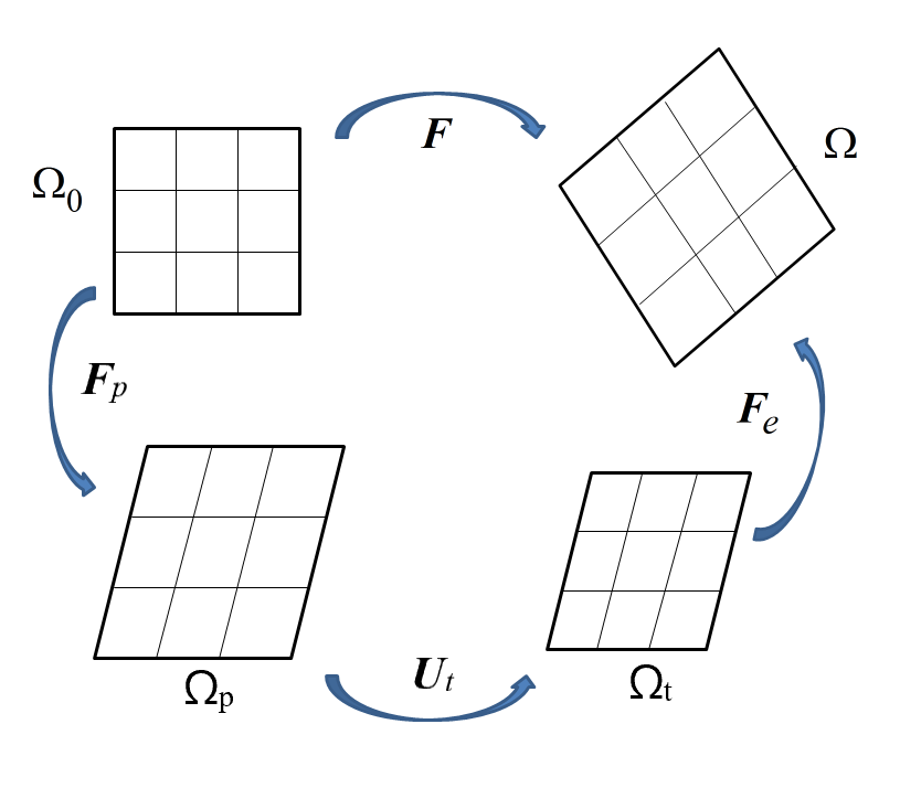
1. Kinematics
1.1. Multiplicative decomposition of the deformation gradient into thermoelastic , transformation , and plastic parts
| (78) |
1.2. Elastic and plastic Lagrangian strain tensors
| (79) |
1.2. Jacobian determinants
| (80) |
where (), (), (), and () are the elemental volumes (mass densities) in the reference , transformed , plastically deformed , and the actual () configurations, respectively.
1.3. Internal time
| (81) |
1.4. Decomposition of the deformation rate
| (82) |
2. Helmholtz free energy per unit mass
| (83) |
3. Elastic energy per unit volume in
| (84) |
where is the fourth-rank tensor of elastic moduli.
4. First Piola-Kirchhoff and Cauchy stress tensor
| (85) |
| (86) |
5. Dissipation rate per unit mass due to plastic flow and variation of the internal variable
| (87) |
6. Dissipative forces for plastic flow and variation of the internal variable
| (88) |
7. Yield condition
| (89) |
8. Evolution equations for plastic strain and internal variables
| (90) |
Application of the same thermodynamic procedure as for small strains but within finite-strain formalism allows us to generalize equations in Box 2 for the dissipation rate due to SC and thermodynamic driving forces for finite strains, see Box 10. Note that in Eq. (96) the transformation work (first term) can be substituted with the corresponding term in Eq. (19).
Box 10. Dissipation rate due to SC and thermodynamic driving forces at finite strains [234, 235, 240, 171, 172, 272]
1. Local dissipation rate per unit mass and dissipative force for structural changes
| (91) | |||||
2. Local thermodynamics driving force per unit mass for complete structural change
| (92) |
or
| (93) |
3. Global thermodynamic driving force for nucleation in a volume , i.e., the total dissipation increment due to SC only during the complete SC in the transforming region
| (94) |
4. Global dissipation rate for nucleation in a volume
| (95) |
5. The thermodynamic driving force for a phase interface propagation per unit reference area
| (96) |
6. Local dissipation rate per unit area for a phase interface propagation
| (97) |
For a particular case when depends on , , and only and for equal elastic properties of phases (i.e., ), surface energy is negligible, for isothermal approximation and homogeneous in the nucleus, Eqs. (93) and (94) result in the following very simplified expression for the thermodynamic driving force for nucleation
| (98) |
Note that in all applications, the term related to was neglected. Algorithms for finite element solutions at finite strains are presented in [171, 263]. Various numerical solutions can be found in our papers [171, 263, 172, 264, 266].
8 Spherical elastic nucleus within an elastic - perfectly plastic sphere
We consider a spherical nucleus of the radius of a product phase within an infinite elastoplastic sphere without strain hardening under action of the external pressure . Such a problem was considered from a thermodynamic point of view using different criteria in several papers, see [192, 110, 239, 393, 111, 112]. To illustrate our thermodynamic approach presented in Box 3 in the simplest way, we will follow [239], where this solution was, in particular, applied to PT from graphite to diamond and to PT in steel. To present the simplest example of our kinetic approach, summarized in Boxes 5-7 , we will sketch the solution from [243, 244].
8.1 Pressure variation and athermal kinetics
We assume (a) a spherical transformation strain with a volumetric transformation strain (negative if compressive) and (b) that isotropic elastic properties do not change during PT for simplicity. Then the pressure in a nucleus is determined by equations from [393]:
| (99) | |||||
| (100) |
Here, are the principle stresses, the elastic constant is expressed in terms of the Young’s modulus and the Poisson’s ratio , is the yield strength of the parent phase, and is the transformation strain corresponding to the onset of plastic deformation in the parent phase. While the equations are valid for any sign of , to be specific, we will discuss SC with compressive under action of compressive pressure . Then, based on Eqs. (99) and (100), the pressure in the nucleus reduces with increasing during the SC. In the elastic region, pressure reduces linearly and can even change a sign. Plasticity retards the pressure reduction. Let us evaluate the transformation work:
| (101) |
in the elastic region and
| (102) |
| (103) |
in the elastoplastic region. Apparently, Eq.(102) reduces to Eq.(101) at (i.e. at ). For simplicity, we will neglect surface energy in this Subsection, assuming a large-size ”macroscale nucleus” (allowing surface energy in this problem to be trivial). Then, substituting in Eqs. (43) and (44) and introducing the thermodynamically equilibrium pressure , we resolve for the PT pressure in the elastic and elastoplastic regimes, respectively:
| (104) |
| (105) |
Thus, the SC pressure may significantly exceed due to the work of internal stresses and athermal threshold . Plastic relaxation decreases the work of elastic internal stresses and, consequently, the SC pressure. Note that Eqs. (104) and (105) at are identical with the solution in [393] but are different from solution in [110] because of different expressions for the thermodynamic driving force. Adiabatic heating due to the SC latent heat and athermal dissipation was considered in [243, 244]. Allowing for adiabatic heating for graphite-diamond (G-D) PT was presented in [246]. Large strain formulation, which also include surface stresses, was applied for sublimation, melting, void nucleation due to fracture, sublimation, and melting and evaporation in [254, 255, 250, 257, 256], see Sections 19.3 and 19.4.
8.2 Phase transformation from graphite to diamond
The obtained solution for a spherical nucleus was applied for interpretation of nontrivial experimental results on PT from graphite (G) to diamond (D) . The equilibrium pressure-temperature line is obtained with the help of chemical thermodynamics [49, 216, 364] is approximated by the following relationship:
| (106) |
In experiments, martensitic PT G-D occurs at significantly larger pressure [49], e.g., at 70 GPa at room temperature. However, in the presence of some liquid metals (e.g., NiMn, Fe, Co, Ni [364]), PT G-D can be observed very close to the equilibrium pressure.
There are numerous theories attempting to qualitatively explain these results by hypothesizing some CRs, catalytic or solvent properties of liquid metals, etc. [216, 364]. It was shown in [239] that our theory with athermal kinetics explains these experiments without involving additional physical mechanisms or CRs.
Based on our theory and numerical estimates, there are three reasons causing the PT pressure in the experiment to significantly exceed the phase equilibrium pressure: (a) the pressure reduction during PT, which reduces the transformation work; (b) the athermal resistance PT ; and (c) the adiabatic temperature increase due to transformation heat released during the short time of martensitic PT.
In the presence of a liquid metal, G dissolves in the metal and recrystallizes from an oversaturated solution as a D when pressure slightly exceeds the G-D phase equilibrium pressure. D grows in an atom-by-atom mechanism from the oversaturated melt. The effect of a liquid is three-fold.
- 1.
-
2.
Second, the pressure variation in the transforming particle within the liquid is negligible because the volume of a liquid is much larger than the volume of a D.
-
3.
Third, the adiabatic process in a nucleus is replaced by an isothermal one due to slow diffusional growth.
Thus, there is no cause for the actual PT pressure to exceed the phase equilibrium pressure. Additional aspects of G-D PT can be found in [239, 246]. Modeling of the industrial process of the D synthesis in a high-pressure apparatus is performed in [262, 365, 225].
One must mention that the above consideration of the G-D PT within the melt was based on the athermal kinetics (as described in Box 3), neglected nucleation barrier, and actual thermally activated nucleation. Due to the large surface energy of a diamond with any surroundings, activation energy for nucleation is very high and the nucleation criterion (54) is not met for experimental temperature. Some possible mechanisms are discussed in [364], but they do not resolve the nucleation problem, either. Thus, the kinetics of diamond nucleation is currently still a mystery.
8.3 Critical nucleus
Let us consider the kinetics of the appearance of a thermally activated spherical nucleus using Box 4. We have
| (107) |
| (108) |
where is defined by Eq.(102) and is independent of radius . According to Eq.(53), maximization of with respect to leads to the critical radius
| (109) |
Substituting into the expression for in Eq. (107), we obtain the activation energy
| (110) |
Then, can be substituted in Eq. (52) for nucleation time and in Eq. (54) for kinetic nucleation criterion. If, for a given the criterion (54) is met, then nucleation time in Eq. (52) is realistic. Otherwise, it is much larger than any reasonable observation time. An increase in reduces the critical radius and mass (volume) of a nucleus and, consequently, activation energy and nucleation time. Classical nucleation theory for elastic materials can be obtained by changing in Eqs. (109) and (110) with the difference in the bulk energy of the initial and final states.
8.4 Macroscale nucleation kinetics
We will start with an approach in Box 5. With Eqs. (107) and (108) for , Eq. (62) specifies to
| (111) | |||
| (112) |
We must also impose
| (113) |
otherwise, either SC is thermodynamically impossible or activation energy for a large enough nucleus is negative. Application of the principle of minimum time (63) with respect to the radius under constraint (113) results in , since nucleation time is a monotonously decreasing function of . Then, we need to switch to Box 6 or 7 and find the thermodynamically admissible radius from the SC criterion , i.e.
| (114) |
Substitution of (114) in Eq.(111) results in
| (115) |
The radius of the thermodynamically admissible nucleus is 1.5 times larger than the critical nucleus (see also Fig. 3). While the activation energy of a critical nucleus is fully determined in terms of and , the activation energy of the thermodynamically admissible nucleus has a fitting parameter , which should be calibrated from a macroscale experiment. Also, the activation energy of the thermodynamically admissible nucleus reduces stronger with the increase in than that for the critical nucleus.
9 Stress- and strain-induced chemical reactions and phase transformations in a thin layer: propagating interface, shear band, and TRIP and RIP phenomena
Problems on an SC in a thin layer in a half-space or space within rigid-plastic formulation allows simple analytical solutions at small strains [238, 240, 243, 244] and large strains [278, 279, 242], in isothermal and adiabatic consideration, for athermal and thermally activated kinetics. These solutions can be applied to analyses of a phase interface propagation, SCs in a shear band and in surface layer caused by friction, and for deriving equations for TRIP and RIP.
9.1 Analytical solution
Consider an infinite rigid-plastic half-space or full-space with prescribed normal and shear stresses on the entire horizontal surface (Fig. 6). Plane strain formulation is assumed both for plastic and transformational strain. We consider an infinite thin layer in which localized SC and plastic flow occur, while the material outside the layer is rigid. Displacements are continuous across the interface, i.e., phase interfaces are coherent. All strain and stress fields are homogeneous within a layer, which also means the total strain represents an invariant plane strain, i.e., shear strain along the layer and normal strain along the normal to the layer. This layer can be obtained by a plane phase interface moving along the normal and producing an SC within a layer, or by localized plastic shear deformation (i.e., coinciding with a shear band) or can be a part of a shear band. Additionally, stresses are assumed to be time-independent (or plastic strain-independent), restricting solution to a perfectly plastic model. The Tresca yield condition is utilized.

For simplicity, we consider a 2D spherical transformation strain with the volumetric strain , while allowing for an arbitrary transformation strain without plane strain assumption is performed in [240]. Geometrically, in Fig. 6a, a transformed Particle, is presented after the transformation strain (which also includes shear). To satisfy the invariant plane strain conditions, an additional plastic strain (TRIP or RIP) further deforms a particle to the configuration shown Fig. 6,b. Adiabatic heating is included in the solution.
Expressions for , for the temperature during and after the end of the SC, and for the effective temperature look as [244, 242, 279]
| (116) |
| (117) |
| (118) |
Here and are the change in internal energy and entropy per unit mass, respectively, is the heat source due to the SC heat , part of transformation work , and TRIP or RIP (see below).
We consider the macroscale kinetics from Boxes 5 and 6. Minimizing the SC time with respect to the thickness of the layer , we obtain
| (119) |
where is the interface area. Maximum in Eq. (119) results in . Then thermodynamically admissible is determined from the thermodynamic SC criterion (66)
| (120) |
With this expression, the kinetic Eq. (67) is
| (121) |
where is the time of deformation in the shear band.
By integrating flow rule, we found the plastic shear , which is TRIP for PTs and RIP for CRs, is determined by the equation
| (122) |
Due to variation in transformation strain (which generates internal stresses and forces plastic strain to restore displacement continuity conditions across an interface), plastic flow takes place at arbitrary (even infinitesimal) shear stress, below the yield shear strength in shear . For relatively small , the relationship between and is approximately linear, as shown in known experimental or theoretical expressions for TRIP [113, 348, 367, 374, 463, 110]. For larger , plastic shear grows faster than linear. The most important property of this solution (which was not present in any previous solutions) is that for (e.g., in a shear band), plastic shear tends to infinity. In reality, it may reach extremely large values, especially for large [276, 213]. It follows from Eqs.(116)-(118) that for the heat source due to TRIP/RIP tends to infinity as well, and the temperature tends to infinity, or to melting temperature, above which the solution does not have a sense. However, if the SC is relatively slow, then the adiabatic condition is not met, and an increase in temperature is much lower. The increase in temperature suppresses martensitic PTs and accelerates some PTs and CRs, which are promoted thermodynamically or kinetically by temperature.
Note that an interesting consequence of a finite-strain formulation is a definite transformation path, i.e., sequences of dilatational and shear transformation strain variation during the PT [242].
9.2 Strain-induced chemical reactions in a shear band
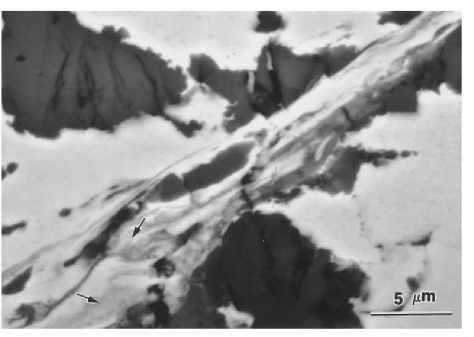
Such exothermic CRs in Ti-Si and Nb-Si powder mixtures were studied in [361, 362], see Fig. 7. The first theoretical modeling of continuum thermomechanical aspects of the problem and interpretation of the possible mechanisms for the promotion of the CRs due to large plastic shear is published in [278, 279, 243, 244]. In these papers, the RIP phenomenon, which is similar to TRIP for PTs, was predicted and used as one of the main accelerators of the CRs. The macroscopic similarity between RIP and TRIP allows one use of the existing knowledge in TRIP [113, 348, 367, 374, 463, 110] for studying RIP. The concept of the effective temperature was introduced as well. Paper [278, 279] has utilized a simplified kinetic equation. In papers [243, 244], a kinetic approach for a macroscale nucleus presented on Boxes 5 and 6 was applied, which led to significantly different results.
One problem of interest was that in [421], an averaged pressure to shock-initiate the CR in mixture was surprisingly low, just several GPa. This was explained by the ”ease of plastic deformation” that leads to improved mixing. However, both materials have quite a high yield strength. The authors assumed the volume change during PTs in and (that occur at a pressure above GPa) promotes the plastic deformation. While the averaged pressure to initiate the CR is just several GPa, however, the authors assume that local pressure in contact between particles may be sufficient for these PTs. As an alternative, it was stated in [278, 279] that since the volume reduction for CR is large, [421], revealed RIP, as a new mechanism of plastic flow in solids, and Eq. (122) may offer more plausible way for interpreting large plastic shear below the yield strength, and how it may reduce stress to initiate CR.
Eq. (121) predicts the exponential influence of and increase in due to RIP on the reduction of the transformation time. The RIP significantly increases the reaction finish temperature , by more than 1500 K, i.e., increases by 750 K. According to Eqs.(116)-(118), increases due to shear stress and corresponding RIP by two macroscopic mechanisms: increase in by 750 K and effective ”reduction” of the yield strength related to satisfaction of the yield condition.
9.3 Mechanochemical feedbacks and the effect of TRIP/RIP on the strain-induced structural changes
TRIP and RIP may cause positive thermomechanochemical feedback. Let a SC occurring fluctuationally in a small part of a layer causing TRIP/RIP. Corresponding heating (if grows with the increasing temperature) accelerates PT and CR, which leads to the intensification of TRIP and RIP and, consequently, of PT and CR, and so on. With such a process, SC can be a cause of shear banding (especially, for the lower yield strength of the product phase) instead of vice versa. This mechanism may be important for solid-gas CR in explosives, e.g., in HMX or nanocomposite formulations [246].
When (i.e., for plastic strain-induced SCs), it is difficult to separate traditional plastic strain due to external loading and TRIP/RIP. This was approximately done, in particular, in high-pressure experiments [275, 276] on PT from the hexagonal hBN to superhard wurtzitic wBN under compression and torsion in a rotational diamond anvil cell. It was found by in-situ x-ray diffraction measurements that the evolution equation for the plastic strain-induced concentration of the turbostratic stacking faults (which is considered as a physical measure of the plastic strain) has two terms. One is proportional to the applied twisting angle (i.e., traditional plastic strain), and the second is proportional to the volume fraction of wBN. The second component was interpreted as the contribution due to TRIP, which was the first revealing of TRIP in high-pressure experiments. It appears that due to the large , TRIP is 20 times larger than traditional plastic strain. TRIP also resolves some puzzles in these experiments, see [275, 276].
Based on recent works on plastic strain-induced SCs under high pressure [247, 246, 252], there are additional reasons for the intensification of SCs due to plastic straining. For the CR, large plastic deformation produces fragmentation and mixing of reactants similar to that in liquid phase reaction [474]. Then plastic straining promotes both PTs and CRs by producing defects with strong stress concentrations (like dislocation pileup or shear-band intersection), like for any strain-induced SCs. This can reduce the PT pressure by one to two orders of magnitude both in the experiment [28, 186, 122] and in the theory or simulations [247, 246, 270, 183, 184, 252]. As a result, a microscale kinetic equation for the volume fraction of a high-pressure phase of the type of
| (123) |
is derived, where is the accumulated plastic strain (Odqvist parameter) defined as , and is the plastic part of the deformation rate. An example of a specific kinetic equation is given in Eq. (167). Such a kinetic equation can be used for the above problem on SC in a shear band to determine evolution of the volume fraction with the increase of plastic shear, instead of determination of transformation time for complete PT. However, it is directly applicable when the plastic strain occurs prior to and during the SC, i.e., for .
The fundamental question arises: should TRIP/RIP be included in the accumulated plastic strain that governs the kinetic equation for ? Based on experiments on PT in BN discussed above [275, 276], TRIP (and, consequently RIP) is not distinguishable from a traditional plasticity from the point of view of dislocation and twinning mechanisms, and the generation of strong stress concentrators at the tip of defects. It is caused by internal stresses produced by the transformation strain combined with the external stresses rather than by solely external stresses. This explains why TRIP/RIP, similar to the traditional plasticity, generates new nucleating defects (along with new turbostratic stacking faults in hBN) that promote the SC. Thus, TRIP/RIP should be included in participating in the kinetic equation for . This, however, was not done in the literature. Note that for temperature-induced PTs, an autocatalytic effect (i.e., formation of a martensitic unit promotes the nucleation of other units via stress- and strain induced mechanism) is an important part of the kinetic equation, see [372].
The entire process represents another positive mechanochemical feedback, which is called in [275, 276] the cascade mechanism of structural changes during the twisting of an anvil. Thus, prescribed plastic deformation produces both turbostratic stacking faults that suppress the martensitic PT, and nucleating defects (e.g., dislocation pileups) that promote the PT. PT under shear stress generates strong TRIP; TRIP, in a similar way as traditional plastic flow, produces the additional turbostratic stacking fault and nucleating defects; the new nucleating defects again promote the PT that induces TRIP, etc.
In [213], the shear transformation-deformation bands have been revealed in the fcc phase of the after compression and shear in an RDAC. The bands consisted of the shear-induced nanocrystals of linearly-polymerized fullerene and polytypes, the triclinic, hcp, and monoclinic, , and amorphous structures. Thus, plastic straining arrests five high-pressure phases under normal pressure, which may be potentially important for their practical applications. Localized shear deformation appears counterintuitive because high-pressure phases of possess greater strength than the parent low-pressure phase. However, this was explained by TRIP during localized PTs, which occurs because of a combination of applied stresses (below the yield strength) and internal stresses due to large volume reduction during PTs. Eq. (122) was used for qualitative analyses. Localized PTs and plastic shear deformation promote each other, producing positive mechanochemical feedback and cascading structural changes. Thus, our solution for a shear band is instrumental for the interpretation of SCs in various systems.
PT of a thin inclined plastic layer. A problem on PT of a thin inclined plastic layer within a rigid-plastic half-space under the action of uniform normal and shear stresses was solved in [238]. The inclination angle was determined explicitly by maximization of the net thermodynamic driving force with allowing for the anisotropy of the athermal threshold . The final expression for the PT criterion was derived. The yield condition for the parent phase was considered as a constraint. The effect of the ratio of yield strengths of the parent and product phases on the PT in the layer was analyzed, and nontrivial behavior was revealed.
10 Phase transition in ellipsoidal inclusion

Consider an infinite elastic space under the horizontal shear stress . It is instructive to solve the simplest problem on the PT within a penny-shape ellipsoidal region with the radius and semi thickness , , within the space, allowing for elastoplasticity within the transforming region, see [244]. Assuming homogeneous fields in and horizontal shear component of the transformation strain only, one can use the Eshelby solution [359] for the shear stress in (Fig. 8):
| (124) |
During the increase in , the shear stress reduces linearly, changing the sense, and at reaches the yield strength in shear in the direction opposite to the applied shear stress. Then, the transformation work is
| (125) |
Both stresses and transformation work are very different than in [378] and [121, 333], where the transformation work was evaluated based on the global or local stress in the nucleus before the PT, respectively, i.e., at for the current problem. We consider the macroscale kinetics from Boxes 5 and 6. Minimizing the SC time with respect to and , we obtain
| (126) |
| (127) |
for determination of the actual and . For and , the principle (126) results in , . Applying these two principles under constraint of the thermodynamic PT criterion or
| (128) |
we obtain
| (129) |
For , the semithickness in Eq.(129) is getting negative. Then the minimum is equal to the lattice parameter in the direction, i.e., . The radius of the macroscale nucleus is determined from the thermodynamic PT condition
| (130) |
Some other cases have been considered in [244]. With known expression for the transformation work, it is easy to find a solution for the critical nucleus using equations from Box 4.
11 Nucleation and growth of martensite with coherent, semicoherent, and incoherent interfaces, and interface with decohesion
11.1 Semicoherent interface and interface with a decohesion
Several types of interfaces will be considered [383]. For a coherent interface displacements, are continuous across the interface (i.e., , where subscripts designate phase 1 and 2), which usually generates large internal stresses. Atomic positions in contacting lattices are continuous across an interface as well. For a semicoherent interface, displacements are discontinuous across the interface, producing relaxation of internal stresses by sliding along the interface (i.e., dislocation generation, in particular, misfit dislocations) and cracks or decohesion (i.e., jump in normal to the interface displacements). It is necessary to note the conceptual difference in definition of interface type for PTs in inelastic materials in continuum and atomistic approaches. At the atomic level, plasticity means there is a presence of dislocations and implies semicoherence. In continuum approaches, plasticity is described in a continuous way and both coherent (with continuous displacements) and semicoherent (with discontinuous displacements) interfaces are considered, see [231, 239, 240, 263, 170].
For a incoherent interface, there is no lattice correspondence across an interface from an atomistic point of view and shear stresses are assumed to be zero in continuum theories. Typical incoherent interfaces appear when one of the phases is molten or amorphous, or for precipitates with a very different crystal structure than the matrix. Due to zero shear stresses at the incoherent interface, incoherent inclusions are under hydrostatic stress states [360, 383, 220]. This is clear for solid-liquid interfaces and is reasonable for solid-solid interfaces under stress-free conditions. Indeed, if there is no correspondence of atomic planes across an interface, the product phase can minimize the energy of internal deviatoric stresses by altering its atomic position within a transforming region. For solid-solid incoherent interfaces under external loading, shear stresses still can be supported by an interface and the assumption of zero shear stress is contradictory. Indeed, incoherent high-angle grain boundaries and interfaces between amorphous and crystalline phases can support shear stresses. At the continuum level, one must use a theory similar to that for the semicoherent interface discussed below with finite maximum shear stress at the incoherent interface. However, stress relaxation for incoherent solid-solid interfaces is more pronounced. It can be described by additional stress relaxation within transforming region rather than at interface.
In material science books [66, 383], spacing between misfit dislocations at the semicoherent interface is introduced from the geometric conditions to completely eliminate the misfit between lattices in the averaged sense. Such spacing is also confirmed within PFA [268, 269] with the stationary solution of the evolving interfacial dislocations. In analytical approaches (see [383, 30, 66, 392]), the initiation of semicoherence in elastic materials was determined by equaling the energy of coherent and semicoherent nuclei with allowing for the energy of dislocations. A semicoherent interface was energetically favorable above some critical nucleus size. The detailed dislocation model of a semicoherent nucleus was suggested in [371, 372]. Continuum derivations of the conditions at an incoherent interface (i.e., assuming zero shear stresses at the interface) were performed in [130, 224, 217, 181, 359, 223, 160] using the energy minimum principle. A sophisticated kinematic approach to semicoherent interfaces was suggested in [50].
It is clear for a semicoherent interface that the glide along the interface is a dissipative process. The dissipation-based approach in the theory of semicoherent PTs within inelastic materials assuming small sliding and in the reference configuration was developed in [231, 239, 263], which was generalized for arbitrary sliding and in the actual configuration in [240]. Since discontinuities at the interface were treated in these works as the contact problem at the moving interface, solutions in the actual configuration were much simpler. It is assumed that SC, interfacial sliding, and decohesion are thermodynamically independent processes which interact through the stress fields only. While in the general theory [231, 239, 240] the change in the free energy due to interfacial sliding was included, it was neglected in all applications. The conditions at the interface are then described by the following equations:
| (131) | |||||
| (132) |
| (133) |
Here and are the shear stress vector and normal stress at the interface; is the critical normal stress for decohesion; and is the tangential to an interface displacements. Function describes the limit curve in the plane of the shear stress , which characterizes athermal resistance to slip, within which relative sliding is prohibited, and is the function that determines the kinetics of sliding. These functions, in general, incorporate crystallographic anisotropy, the magnitude of sliding rate, and , as well as other features from the theory of crystal slip or discrete or continuously distributed dislocations [155, 39, 10]. The relative sliding can characterize continuously distributed dislocations [155, 39] within an interface and number dislocations is equal to divided by the magnitude of the Burgers vector . The description of the interfacial sliding is formally similar to the flow theory in plasticity, where is for the yield surface and is for the flow rule. In particular, in [231, 240] an associated sliding rule was derived using the extremum principle similar to that in plasticity, that was derived using the postulate of realizability.
Remark. Note that such a continuum description of the incoherence does not completely reflect real dislocation processes, because the Burgers vector of dislocations and their sliding are limited to the interface only, which is typical for misfit dislocations. In general, the Burgers vector and sliding can be inclined to the interface and dislocations may slide together with the propagating interface (glissile interface), thus producing much less resistance to the interface motion than the misfit dislocations.
For isotropic functions and Eqs. (131)-(132) simplify to
| (134) | |||||
| (135) |
where is critical shear stress (or athermal threshold) for sliding and is a scalar, which is determined from the condition . Note that the last condition corresponds to the main equilibrium equation for continuously distributed dislocations [155, 39].
If during the increase in and changing thermomechanical properties in a nucleus, a chosen decohesion condition is satisfied in some point of the interface, the crack appears or grows. If during the same process the sliding criterion is met, we admit glide in this point up to a value, at which the criterion is violated. After finishing the SC, we use the SC criterion to determine if SC is a thermodynamically admissible process.
11.2 Propagation of a semicoherent interface
Propagation of coherent and semicoherent interfaces in elastic and elastoplastic cylinders under an axial stress of 100 MPa is investigated in [170, 263, 172], see Fig. 9 for a semicoherent interface. Interface propagation is simulated by layer-by-layer transformation. For a coherent interface in an elastic material at , the transformation work grows for each next layer, i.e., after PT in the first layer propagation should occur with increasing velocity. Phase equilibrium could be achieved if grows sufficiently with the growing volume fraction of the product phase or if it is distributed heterogeneously. For a semicoherent interface, it is assumed that the sliding displacements (dislocations) at the layer’s interface do not vary after finishing PT in the layer, so they represent a memory about semicoherent PT. Discontinuity in displacements causes discontinuity in pressure (Fig. 9) and all stresses except normal and shear stresses at the interface. We did not consider further sliding within the product phase, assuming that the yield strength in shear is much larger for inherited dislocations, because in most cases dislocations do not belong to the main slip systems of the product phase. Sliding of dislocations inherited by propagating interface is taken into account within PFA to the interaction between the PT and dislocations in [269, 271, 182].
Stress relaxation due to semicoherence increases and consequently the driving force for PT in the first layer; i.e., PT can start at a higher temperature than for the coherent interface. The transformation work slightly grows for PT in the second layer, i.e., the interface will propagate at a fixed applied stress and temperature. However, the driving force for the PT in the third layer is smaller than for the first layer, and it continues decreasing for the fourth and fifth layers. Thus, there is a tendency for interface arrest because of stress relaxation due to semicoherence.
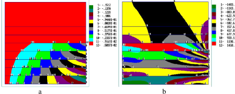
Next, after PT in the first layer, the second and third layers were compared as the next transforming region [263], based on the extremum principle (47). For a coherent interface, continuous interface propagation through the sample was obtained. For a semicoherent interface, the transformation work was larger for PT in the third layer (for relatively small ), which leads to formation of discrete martensitic microstructure. Thus, a semicoherent interface has lower mobility than a coherent one and can be arrested more easily, in accordance with experiments.
Plastic deformation in the parent phase in this problem was considered in [170, 263, 172]. For a semicoherent interface, plastic deformation is quite small and weakly affects PT because is much smaller than the yield strength in shear. For a coherent interface, plasticity, as the stress relaxation mechanism, produces effects similar to those for sliding along the interface. Thus, plasticity increases the transformation work for PT in the first layer (in comparison with elastic parent phase) but then leads to PT in the third and fifth layers, leading to a discrete martensitic microstructure and possible arrest of the interfaces.
The effect of strain hardening, leading, according to Eq. (49), to the increase in the athermal threshold , was analyzed in [170, 172]. Since plastic deformation and increased are localized more near an interface, it promotes the formation of a discrete microstructure. Note that different scenarios of interface propagation strongly depend on the chosen material parameters (, , , , etc.) and applied stresses.
11.3 Stress-induced PT in a spherical particle within a matrix and its interaction with plasticity, semicoherence and adhesion
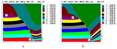
Following [263], we will present results for PT with volumetric transformation strain within a spherical particle embedded in a nontransforming cylindrical matrix (Figs. 10 and 11) at a fixed temperature and compressive axial stress . Solutions are found for coherent and semicoherent interfaces and an interface with decohesion, with different magnitudes of and . Examples of discontinuity of displacements for a semicoherent interface and an interface with decohesion are shown in Fig. 10. The averaged mean stress and transformation work as functions of transformation strain for different interface conditions are presented in Fig. 11. The mean initial compressive stress in a sphere of reduces in magnitude and changes the sign during PT (increase in ) due to internal stresses, which reduces the transformation work and makes it negative for a coherent interface and semicoherent interface with . Interfacial sliding and decohesion relax internal stresses and increase the transformation work. Remarkably, initiation of decohesion leads to a large drop in tensile mean stress in a particle and a corresponding sharp change in slope of the plot for . Thus, the minimal and consequently the driving force for SC is for the coherent interface, the maximum is for . However, even for the stress state in a spherical particle is nonuniform and nonhydrostatic, so it can hardly be called an incoherent inclusion. The interface with decohesion shows the second largest transformation work.
Let us assume that the external stress is small enough (in particular, zero) to cause plasticity, semicoherence, and decohesion without PT. We can choose a temperature at which PT criterion (43) is not met without plasticity, semicoherence, and decohesion, because the transformation work is too small without stress relaxation. Thus, none of the inelastic processes can occur separately under the chosen conditions. At the same time, when at least two inelastic stress relaxation mechanisms proceed simultaneously, they assist each other via the field of internal stresses, relax internal stresses, and can all occur thermodynamically and based on sliding, decohesion, and/or yield criteria.
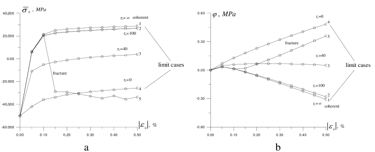
11.4 Semicoherent interface within a phase field approach
The first work on introducing incoherence in the diffuse interface within PFA was presented by [6]. Because of the finite-width interface, localized sliding was substituted with additional eigen strain fields within an interface that relaxes interfacial shear stresses. An additional order parameter for the description of incoherence is introduced, which is equal to zero and one for the coherent and incoherent interfaces, respectively. The evolution equation for the order parameter is derived thermodynamically, and the driving force for the evolution of incoherence is the shear stress along the interface minus the change in the interfacial energy due to change in the order parameter , which was approximated by some function. From a thermodynamic point of view, the theory in [6] is the finite-width counterpart of the theory for sharp interfaces in [231, 240]. At the same time, change in the interfacial energy with incoherence was taken into account in the solution of all problems, which eliminated complete relaxation of the shear stresses. However, function was not included in the expression for the interfacial energy that governs the evolution of the main order parameter describing evolution of the two-phase system. This did not affect correctness of the results of the solution of various problems for different geometries of the interfaces in [6] because they were presented for fixed interfaces only. Also, results were presented for the stress-free external surfaces, i.e., the problem of the finite strength for the incoherent interfaces was not discussed.
11.5 New approach to incoherent interface
A method to relax stresses within the moving finite-width solid-melt interface within PFA was suggested in [283]. While displacement continuity was assumed, due to the zero shear moduli of the melt, deviatoric stresses in the melt are zero. The problem was that stresses within the finite-width interface, within which shear modulus varies from that for a solid to zero, due to the traditional pure spherical transformation strain for solid-melt PT, , were unreasonably high. This did not allow for reproduction of the experimental size dependence of the melting temperature of the Al nanoparticle and temperature-dependent thickness of the surface molten layer. To reduce interfacial stresses, the deviatoric part of the transformation strain, was introduced, which evolved according to thermodynamically consistent evolution equation during the PT
| (136) |
where is the kinetic parameter and is an interpolation function of the order parameter for the volumetric transformation, , . This led to significant reduction of the interfacial stresses, controlled by a kinetic parameter , and the quantitative description of the above experimental data for Al.
A similar approach was developed in a thermodynamic theory in [288, 297] to relax internal stresses during a diffusion-driven compositional expansion/contraction in an amorphous material, in particular, during the lithiation-delitiation of silicon. Instead of the isotropic compositional expansion typical for an isotropic amorphous material, anisotropic deviatoric-stress-dependent compositional expansion was introduced and described by the following equation
| (137) |
Here, is the deviatoric part of compositional deformations rate, is the third invariant of the compositional part of the deformation gradient (which describes volumetric compositional expansion) as a function of concentration of saturating atoms, . This led to obtaining very good correspondence with experimental and atomistic results on the biaxial stress relaxation in on a rigid substrate in the course of lithiation-delithiation, utilizing just a single fitting kinetic parameter .
The results obtained allow us to conceptually reconsider the definition and way of description of the incoherent interfaces in solids, in order to include finite shear strength at least after transformation with strong stress relaxation during PT or chemical reaction. Since there is no atomic correspondence across an incoherent interface, it is unphysical to describe this process through dislocation generation or sliding along the interface. We postulate that the lack of atomic correspondence across an incoherent interface is due to the reconstructive atomic motion in the transforming volume covered by a moving interface. Then we keep displacement continuity across an interface but add a mechanism of stress relaxation within the transformed phase by introducing a deviatoric-stress-dependent deviatoric part of the transformation strain rate, described by equations of the type of Eqs. (136) or (137), for the PFA, or description in terms of volume fraction of phases or concentrations of the diffusing species, or the sharp interface approach. Then the internal deviatoric stresses significantly (or almost completely) relax during PT or reaction, but after stopping transformation, the two-phase material and incoherent interface can carry deviatoric stresses, which are determined by plasticity/strength of bulk phases and interfaces.
11.6 Semicoherent interface within a phase field approach with discrete dislocations
While PFA to coupled PTs and discrete dislocations will be described in more detail in Section 16.5, here we will focus on semicoherent interfaces [268, 269]. Initially, a stationary solution for the coherent finite-width austenite-martensite interface was obtained (Fig. 12a) with a misfit strain along the interface . The coherent interface could be kept stationary at some temperature close to the phase equilibrium temperature (and corresponding normalized thermal driving force ) for a stress-free material, see the red line in Fig. 12b designated as . This small deviation is caused by nonsymmetric sample geometry due to dislocations and energy of internal stresses, which, due to small sample size, slightly depends on the interface position. At any other temperature, the interface propagates until completion of direct or reverse PT, depending on the temperature, which was not a surprise. It is known (see [273, 274]) that PFA for PTs does not include an athermal threshold to the interface propagation, and one needs to develop some special ways (e.g., oscillating distribution of internal stresses or some heterogeneities) to introduce it into PFA.
Internal stresses due to a misfit strain led to nucleation of the misfit dislocations at the intersection of the interface with a sample free surface, which propagated along the interface producing the stationary distribution of dislocations. Equilibrium spacing between misfit dislocations, , was found to be in perfect agreement with an analytical expression .
For a semicoherent interface, temperature and normalized thermal driving force can be varied in some range, limited by the critical values for martensitic PT and for martensiteaustenite PT (Fig. 12b), without interface motion. These critical values of represent an athermal threshold (or interfacial friction) for the interface propagation due to misfit dislocations. After exceeding these thresholds, the entire sample transforms into a single phase–austenite or martensite–for different signs of . What is very surprising is that the athermal thresholds strongly depend on the ratio of two nanosize parameters , where is the interface width and is the dislocation height, see Fig. 12b. Indeed, the athermal interfacial friction is a macroscale characteristic which can be measured in a macroscale test on a single or multiple interface propagation, and for macroscale treatment all nanoscale parameters are usually neglected. However, the dimensionless ratio of two nanosize parameters is a finite number and, according to Fig. 12b, should be taken into account even in the macroscale treatment. Also, (almost) zero athermal friction for very small and for is a very nontrivial result. The obtained result that the athermal hysteresis for a broad enough interface is zero is intuitively acceptable, because the resultant driving force from the interaction of all infinitesimal layers, producing the broad interface, with ”thin” misfit dislocations disappears due to mutual compensation. Since the dislocation height is approximately equal to the crystal lattice parameter, this result also implies that for broad enough interface the Peierls barrier due to discreteness of the crystal lattice tends to be zero as well.
However, the case for an (almost) sharp interface looks contradictory and requires further study. Indeed, for 1D plane interface propagation through the oscillating stress field, which was used in [273, 274] in order to introduce an athermal barrier in PFA, the hysteresis was finite and was determined by extreme (positive and negative) values of the oscillating stresses. Since dislocations also produce the oscillating stress field, the same is expected for the interactions of very thin interfaces with dislocations. One of the possible reasons of this discrepancy is that in [268, 269] the interface does not move as a plane. Instead, the thin interface penetrates between dislocations, pushes them away, increasing spacing between dislocations, and finally loses its stability and propagates laterally through the entire sample (Fig. 12a). The finite size of the sample may contribute to this phenomenon, so larger scale simulations are required.
Note that many other examples within PFA were found for which the ratio of two nanoscale parameters (e.g., the width of two different interfaces or width of the interface and the external or internal surfaces) drastically affects PT nanoscale and macroscale behavior, see review by [251]. This ratio produces new phenomena, changes PT parameters and mechanisms, and should be considered as a new dimension in a ”phase diagram.” Additional examples include PT between two solids via an intermediate phase (melt) and surface-induced melting of nanoparticles and martensitic PTs.
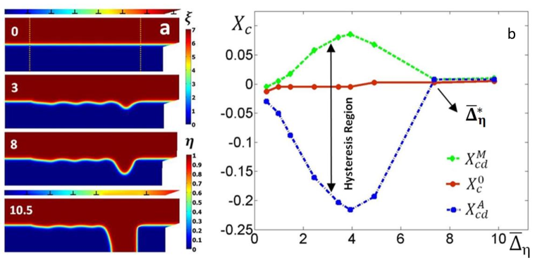
While the results above were limited to misfit dislocations that nucleate and evolve along the interface only, a more general situation was treated in [270, 183, 184], where dislocations move along the natural slip system of evolving phases. In those examples, one of the initially coherent phase interfaces adjusted itself to the stress field of a dislocation pileup, and a high-pressure phase was arrested at the dislocation side with an extra atomic plane because it could not propagate to the side with missing atomic planes and tensile pressures (Fig. 22). The results for this interface are quite similar to those for the interface with misfit dislocations.
An alternative approach to the coherency loss of the stationary spherical precipitate with volumetric transformation strain using PFA to discrete dislocations was suggested by [124]. Their PFA is developed in terms of shear strain along the specific glide planes and directions as order parameters. Periodic dependence of the energy on this shear strain is accepted, which allows to reproduce punching of prismatic dislocations with edge and screw components from the precipitate. While small strains are assumed, it is written that generalization for finite strains is not a problem.
12 Solid-solid phase transformations via intermediate (virtual) melt
When traditional mechanisms of plastic relaxation of elastic stresses through dislocation motion and twinning are inhibited, nature finds alternative ways to relax internal stresses. Thus, solid-solid PTs through a nanometer-size liquid layer, hundreds of Kelvins below the bulk melting temperature, was predicted by continuum thermodynamic estimates and confirmed directly or indirectly in experiments for various material systems, see [260, 249, 261, 281, 38]. Instead of traditional propagating solid 1- solid 2 () interface, solid 1-intermediate melt-solid 2 () interface propagates through material with a thin layer of melt (Fig. 13a). This means that the solid partially or completely melts and recrystallizes into . Complete (or partial) melt within PFA for melting means that the order parameter describing melting and varying between 0 for bulk melt and 1 for solid, is equal to 0 (or is between 0 and 1). Complete melt fully relaxes deviatoric stresses, which appear at interface due to transformation strain. This reduction in elastic energy due to melting increases the thermodynamic driving force for melting and leads to melting below the bulk melting temperature. transforms a coherent stressed interface in a stress-free noncoherent interface. Since melt does not interact with the stress field of defects and does not possess a Peierls barrier, the athermal friction . Elimination of elastic energy and athermal friction may lead to PT with zero transformation hysteresis and energy dissipation, which are ideal property for shape memory alloys for actuation or medical applications [77, 62, 408] or caloric materials [408, 420, 158].
Another reason for melting significantly below the bulk melting temperature is the reduction in the total interface energy, i.e. when the energy of two solid-melt interfaces is smaller than the energy of a coherent solid-solid interface. There is the following difference between the and virtual melt (). The is thermodynamically stabilized by a reduction in surface and elastic energies and can exist for a resting interface. The is an unstable transitional phase along the transformation path between two solid phases. It disappears in a material point quickly after it appears, and does not exist in the stationary interface but can exist within a propagating interface. Short review of the virtual melting phenomena is given in [287]; see also [251].
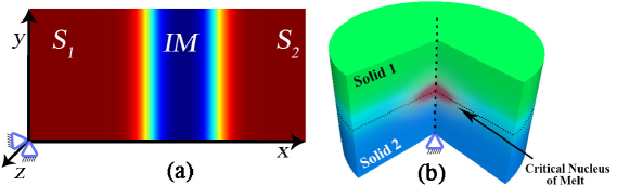
Below are some examples of solid-solid PTs via virtual or intermediate melt.
(a) The concept of the virtual melt was first introduced for the description of numerous counterintuitive experimental results for reconstructive PTs in the organic energetic crystals HMX [260, 261], which were considered major puzzles for decades. In total, sixteen theoretical predictions based on are in qualitative and quantitative agreement with experiments [260, 261, 304]. In particular:
- melting could indeed occur 120 K below the melting temperature. The energy of internal stresses due to volumetric transformation strain is sufficient to reduce the melting temperature from 551 K to 430 K for the phase during the PT studied at 430 K and from 520 K to 400 K for the phase during the reverse PT. Change in surface energy was neglected.
- Zero energy of elastic internal stresses and athermal friction for both PTs explain the experimentally observed lack of the temperature hysteresis, which usually exists for all known solid-solid PT.
- Activation energies for direct and reverse PTs are equal to the corresponding melting energy. Temperature dependence of the rate constant is determined by the heat of fusion, both like in the experiment.
- Kinetics of phase interface propagation and a physically-based kinetic model in terms of volume fraction of the phase are in good correspondence with experiments (Fig. 14).
- Nanovoids in the transformed material that accompany the PT do not affect the PT thermodynamics and kinetics for the cyclic PTs, like in experiments.
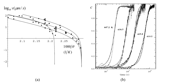
Kinetics of - PT in HMX was also explained by , but a reduction in interfacial energy during PT was involved as well [38].
(b) Virtual melting was suggested as the mechanism for crystal-crystal and crystal-amorphous PTs in materials with melting temperature decreasing with pressure, e.g., in Si, Ge, ice, geological material (e.g., quartz and coesite), and superhard materials (hexagonal BN and graphite) [249]. When pressure-induced PT of phase 1 to phase 2 is suppressed due to large transformation strain and athermal friction, with increasing pressure, the melting line extrapolated to lower temperatures can be crossed before the line for PT . After phase 1 melts, the melt finds itself in the region of the phase-temperature diagram, much below the melting temperature of phase 2. Therefore, material solidifies in a stable phase 2. Below the glass formation temperature, solidification occurs into the amorphous phase, and above the glass formation temperature, crystalline phase 2 appears. An alternative scenario consists of the nucleation of phase 2, which causes large internal stresses, which relax via followed by solidification into amorphous phase 2 (amorphization via internal stress induced ). This model was applied to the explanation of melting, crystal-crystal, and crystal-amorphous PT mechanisms in ice Ih. Note that the occurs in Si and Ge at a temperature of more than 1000 K below the thermodynamic melting temperature!
(c) A new mechanism for crystal-crystal PTs via surface-induced is justified thermodynamically and confirmed experimentally for the PT in nanofibers [281]. For nanofibers, surface melting starts at a temperature much below the bulk melting temperature. When the thickness of the surface melt exceeds the size of the critical nucleus of the product-phase, nucleation, and growth of the product phase takes place. For nanofibers, surface melting starts near the smallest size, and hydrodynamic flow caused by a reduction of the external surface and, consequently, its energy leads to a large shape change towards a cube and additional promotion of crystal-crystal PT. In the course of the product crystal growth, is experimentally observed within the crystal-crystal interface using transmission electron microscopy.
Two different PFAs to the were developed using two order parameters: one describing solid-solid PT and another one for melting, see Fig. 20(c) for approach in [351, 277, 353, 354] and Fig. 20(f) for approach in [282], as well as Sections 16.2.3 and 16.2.5 for details. Also, papers [277, 352, 353] include coupling with elasticity and [354] include interfacial stresses. Internal elastic stresses promote the existence and persistence of the . In particular, in [352], the internal stresses decreased the activation energy of critical nucleus (Fig. 13b) by a factor of 16 for the HMX, making thermally activated nucleation of the possible.
PFA solutions and obtained nanostructures, in addition to expected parameters, like the ratio of energies of solid-solid to solid-melt interfaces and initial state, were found to strongly and nontrivially depend on the ratio of widths of solid-solid to solid-melt interfaces, . Depending on (and other parameters), several types of behavior are found:
(a) for small , jump-like (first-order PT) nucleation of the interfacial disordering and then continuous (second-order PT) and reversible increase in disordering with temperature;
(b) for larger , coexistence of and nanostructures and jump-like PTs between them for increasing and decreasing temperature;
(c) retaining of as a metastable interfacial phase significantly below the bulk melting temperature, even when the energy of solid-solid interface is smaller than the energy of two solid-melt interfaces, and
(d) unstable , which is a critical nucleus between and nanostructures (Fig. 13b). Increase in suppresses barrierless nucleation but promotes retaining of at much lower temperatures.
There are various follow-up works on virtual melting. Amorphization via virtual melting in Avandia (an important antidiabetic pharmaceutical) was proved experimentally using microcalorimetry [384]. Chemical reaction transforming Si into SiC via intermediate state, consisting of dilatational dipoles in Si, was independently studied in [212], including developing PFA.
Convincing direct experimental proof that some reconstructive crystal-crystal PTs (namely, the transition between square and triangular lattices of colloidal films of microspherical particles) can occur through nucleation via an intermediate liquid nucleus and grow via an intermediate liquid layer that was presented in [379]. While it is stated in [379] that crystal-crystal PT occurs below the bulk melting temperature , the bulk thermodynamic force for melting is considered to be positive. This is possible only if the temperature is above the of the phase and below that for the phase. In this case, it is not surprising that when both melting and crystal-crystal PT are thermodynamically possible, the nucleus with smaller activation energy (and, consequently, interface energy) appears first and then transforms to a more stable phase.
Also, this work was not be properly placed within the existing literature. Opposite to the statement in [379], PTs between crystalline phases via intermediate and virtual melting were discussed for a decade and under much more surprising conditions, namely, significantly below the , see the references in this Section. Processes observed in [379] and thermodynamic treatment are identical to particular cases of those discussed in [249, 281]. PFAs to the discussed above are, of course, much more powerful and informative than sharp interface approaches. Additionally, it is stated in [379] that the effect of anisotropic stresses on intermediate melt is worthy of study. This topic was addressed in [280], where in Al and Cu below the under very high-strain-rate uniaxial compression was predicted thermodynamically and confirmed by MD simulations, see Section 13.
Despite these drawbacks, the results in [379] make valuable contribution by direct confirmation and visualization of the crystal-crystal PT via for reconstructive PT in colloidal films. They in-situ confirm, specify, and quantify main statements in [260, 249, 261, 281, 351, 277], including fast growth kinetics for interface (consistent with the absence of the athermal friction) while a coherent crystal-crystal interface is arrested due to the athermal threshold.
Void nucleation due to sublimation within elastoplastic material via is considered thermodynamically and kinetically in [255] and is compared with other scenarios (due to fracture, sublimation, and melting, and evaporation) in [256].
Some other processes that may occur via and virtual amorphization, namely crystal reorientation during the nanofriction via the [148], plastic deformation at a high-strain-rate tension of metallic nanowires via the virtual amorphization [173], fracture [366, 320], and grain boundary sliding and migration [356, 399, 455] are discussed in [287].
13 Virtual melting as a new mechanism of plastic deformation and stress relaxation under high strain rate loading
Generation and motion of dislocations, twinning, and crystal-crystal PTs are the main mechanisms of plastic deformation and relaxation of non-hydrostatic stresses that are reflected in the deformation-mechanism maps [120, 340].
Several large-scale non-equilibrium MD simulations for metallic fcc single crystals found unexpected result that for propagation of a shock wave along the 110 and 111 directions, melting occurs at temperatures below the equilibrium melt temperature at the shock pressure ; for example, for Cu by 20% in [387] and by 7-8% () in [5]. Usually, traditional superheating is observed. This suppression in was interpreted in terms of solid-state disordering due to high defect-densities, but significant dissatisfaction was remained. The decrease in the melting temperature caused by deviatoric stresses was estimated by traditional approaches [130, 400] to be just 1 K. That is why it was not considered for interpretation of results in [387, 5].
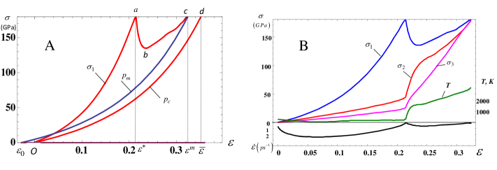
We proposed in [303, 280] the as a new plastic deformation and deviatoric stress relaxation mechanism at temperatures thousands Kelvin below . Thermodynamics of melting under homogenous uniaxial deformation (equal to volumetric strain; in a planar shock, lateral strains are absent) was developed as a generalization of the approach in [240, 243] for melting, see Boxes 1 and 2. Stress-strain curves required for evaluation of the thermodynamic driving force for complete melting were obtained from quasi-isentropic MD simulations (Fig. 15). Surface energy and dissipation were excluded. Temperature increase after initiation of melting (Fig. 15B) was neglected, underestimating . The condition after some transformations leads to the following expression for the equilibrium melt temperature under uniaxial straining :
| (138) |
where all parameters and geometric interpretation are given in Fig. 15A. The magnitude of the negative mechanical part of the thermodynamic driving force for melting under hydrostatic pressure is equal to the area between the equation of state for melt and crystal . This area characterizes the increase in the melting temperature for Cu under hydrostatic loading from to . The difference between the areas under the stress-strain curve and the equation of state of the crystal provides an additional driving force for melting due to non-hydrostatic loading (the term in parentheses in Eq.(138)). This area is about three times of the area and produces about three-fold reduction in in comparison with the raise due to the hydrostatic pressure.
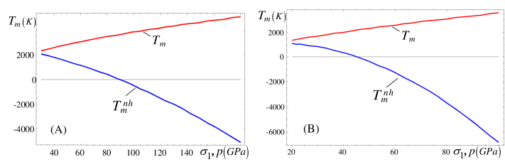
The reduction in the thermodynamic melt temperature based on Eq.(138) is presented in Fig. 16, and it is enormous at high stresses, like .
The above derivations are applicable for perfect crystal when dislocations and twins do not have time to nucleate, or for crystal with some defects, which produce stress relaxation slower than melting, i.e., at high strain rate of 109-1012 s-1 and higher. At lower strain rates, traditional dislocation or/and twinning plasticity takes place. Since melting occurs on the ps time scale, significant overheating is required. Melting starts when crystal lattice loses its stability, with assistance of thermal fluctuations. Numerous MD simulations in [303, 280] have confirmed the at least at , i.e., 4000 K below for Cu for 110 loading and even at (i.e., at 300 K) for isothermal 111 loading of defective Cu. After melting, deviatoric stresses relax and hydrostatically loaded melt is deeply in the region of stability of a solid phase. Melt recrystallizes at ps time scale. Since competes with traditional defect-based mechanisms, it should be incorporated in the deformation-mechanism maps [120, 340] for strain rates of s-1 in metals, and high shear stresses. For materials with inhibited plasticity (covalent crystal Si, Ge, SiC, high-strength materials and alloys, or complex organic molecules like HMX), VM may be observed at lower strain rates and stresses.
The VM phenomenon in a shock wave was confirmed and further elaborated in MD simulations for single crystal Cu, Al, Ta, Pb in [46, 151, 441, 443] and for polycrystalline Be in [84].
In [303] virtual amorphization was suggest as the first stage of . Difference between amorphous and liquid phases from mechanical point of view is that amorphous phase has finite shear modulus and yield strength, which are both zero for liquid. After crystal lattice instability and initiation of disordering at strain (Fig. 15), material still keeps the yield strength (difference between and two other stresses) and crystal anisotropy (difference between and ). For strain exceeding strain, for which , material is completely disordered and isotropic but keeps the yield strength, i.e., it is amorphous solid. It is unstable and transforms with further loading continuously (i.e., via second-order transition) to VM, when all three stresses are getting equal.
For different materials (e.g., organic -HMX crystal, Si, SiC, and ) plastic deformation in shock or dynamic loading occurs by generation and motion of dislocations or twin boundaries up to some pressure or strain rate and via formation of amorphous shear nanobands at higher pressure or strain rate [180, 145, 469, 470, 471, 472, 318]. This amorphization may occur via VM, like pressure-induced amorphization in [249]. Since free energy of melt is usually considered equal to the free energy of amorphous phase, thermodynamic theory developed in [280] can be applied for uniaxial loading or modified for other loadings.
14 Strain-induced nucleation at shear-band intersection. Application of the global criterion for structural changes
The main experimental results on strain-induced PTs in TRIP steels [369, 367, 370] can be summarized as follows:
-
1.
Intersections of the shear bands serve as the main nucleation sites;
-
2.
PT takes place during the shear-band intersection process;
-
3.
Subsequent growth of the martensite beyond the shear-band intersections is quite restricted;
-
4.
Not every shear-band intersection causes martensite nucleation.
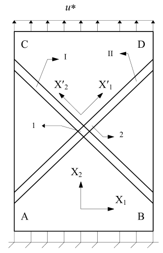
Problem of PT at shear-band intersections with athermal kinetics presented in Boxes 2 and 3 was formulated and solved at finite strains in [264]. The schematics of the sample with prescribed vertical displacement as the boundary condition is shown in Fig. 17. Two orthogonal shear bands are introduced as the regions where material deforms plastically, while deformation is elastic in the rest of the sample. The yield strengths of the austenite and martensite, as well as transformation shear and normal strains in an invariant-plane strain are:
| (139) |
Normal and shear directions of an invariant-plane strain were directed along the shear bands, because this corresponds to the maximum of the transformation work. Transformation strain is introduced in the nucleus proportionally to the increasing displacement , for several maximum displacements . By dividing by the initial length of the sample , we can characterize prescribed displacement in terms of averaged vertical strain .
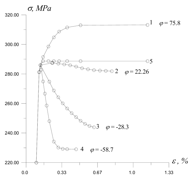
Dependence between averaged axial stresses and vertical strain , for different during which complete PT in a nucleus occurs, is presented in Fig. 18. The values of the calculated transformation work are shown near each curve. Stress-strain curve 5 corresponds to the deformation without PT, and we will call the corresponding stress a macroscopic yield strength of an austenitic sample. For known temperature and , one determines the required transformation work from the PT criterion (43)-(44) and finds with the help of Fig. 18 at which PT may occur. However, as we discussed in Section 6.6, the solution without PT is also acceptable, since all equations of continuum thermomechanics are met. Based on the global stability criterion (50), we conclude that if curve for the solution with PT is higher than the the macroscopic yield strength without transformation 5 (like the curve 1 in Fig. 18), the transformation is impossible, despite the potential fulfilment of the thermodynamic PT criterion. Thus, deformation will occur along the curve 5. In the opposite case (for curves 2 - 4 in Fig. 18), the deformation-transformation process with PT will be realized. This problem represents one of the nontrivial applications of the global SC criterion based on the stability analysis.
It was found that the transformation work is much lower (a) when nucleation occurs at any other place but shear-band intersection; (b) nucleus grows beyond the shear-band intersection, and (c) if nucleation occurs after shear-band intersection without PT at fixed or . These findings explain the experimental results in items 1 to 3 above.
Next, the same loading and processes were considered for the sample, consisting of four samples shown in Fig. 17 connected consecutively in the vertical direction. While all four shear-band intersections are fully equivalent, we consider four cases with one to four nuclei that appear during the same prescribed . The transformation work reduces with the increasing number of nuclei at shear-band intersections. However, for a single nucleus, which can appear for the prescribed at the highest temperature, stress-strain curve exceeds that for the deformation without PT. That means that such a PT is impossible due to the global SC criterion (50). However, for multiple elements, such a PT is also impossible because plastic flow in the untransformed shear-band intersections does not allow stresses above the macroscopic yield strength of an austenitic sample. Thus, the treatment of the sample with the multiple samples shown in Fig. 17 connected in series gives us the corroborating arguments for the validity of the stability analysis and the global SC criterion based on the extremum principle (50).
Since the transformation work reduces with the increasing number of nuclei at shear-band intersections that appear during prescribed , this results in appearance of one nucleus during part of the prescribed , for which the thermodynamic PT criterion is met, and stress does not exceeds the macroscopic yield strength for the austenite. Within next strain increment , the stress increases and reaches the macroscopic yield strength for the austenite, and then nucleus appears at other shear-band intersection, and so on. The maximum temperature for the strain-induced PT, , corresponds to the process, for which nucleation of a single nucleus occurs during that gives the stress-strain curve slightly lower than the macroscopic yield strength of the austenite. That means that is determined not by thermodynamics (since the larger transformation work can be obtained), but by the impossibility of PT due the global PT criterion based on stability analysis.
Thus, experimental phenomena 1 to 4 enumerated at the beginning of this Section are at least qualitatively described by our theory presented in Boxes 2 and 3 without involving additional physical mechanisms. More quantitative description should include discrete dislocations or twin bands or -martensite bands, leading to high stress concentration due to difficulty to transmit shear band through the intersecting band.
It was also found in [264] that the transformation work is a function of the ratio , where is an increment of the volume fraction of strain-induced martensite. For macroscopically uniaxial strain, is the accumulated plastic strain . This finding led to the thermodynamic derivation in [247, 246] of the microscale kinetic equation for the volume fraction of a plastic strain-induced high-pressure phase of the type of Eq. (123), see example in Eq. (167).
Simulations show a significant difference between transformation conditions for displacement- and stress-controlled loadings. For prescribed stresses, the more martensite is, the larger the overall transformation strain and work are. The principle of the maximum transformation work results in the complete transformation in the entire band, without plasticity. Thus, stress-induced PT produces a plate-like nucleus, in contrast to strain-induced PT, which corresponds to known experiments. The adiabatic heating and its effect on PT at the shear-band intersection was analyzed in [172].
Stability analysis should be applied for any problem with boundary conditions in displacement, when PTs competes with plasticity. For example, similar treatment was performed for PT in a spherical particle imbedded in a cylindrical sample [172]. The extremum principle for determination of the stable deformation process is applicable for the analysis of the competition between other inelastic mechanisms, e.g., twinning, damage, and others. For the softening behaviour during PT, the stability analysis plays significant role for the PT in elastic materials as well, see [230, 231].
15 Appearance and growth of a martensitic plate in elastoplastic material
15.1 Macroscale nucleation of a martensitic plate
Appearance of a small rectangular (in the reference state) temperature-induced martensitic plate of the length and height within a much larger rectangular austenitic sample was studied in [171, 172] for finite elastoplastic and transformation strains. Plane-strain formulation and the invariant plane transformation strain with shear along the length were considered. The transformation strain and the yield strengths are given in Eq. (139). Incrementally increasing the transformation strain components and solving the corresponding elastoplastic problem, the transformation work was evaluated and approximated as
| (140) |
The martensitic plate deforms elastically except of narrow regions near short sides. In the austenite the plastic strains are localized around the transformed plate (Fig. 19(a)). The ”macroscale” thermally activated kinetics presented in Boxes 5 and 6 was applied. The principle of the minimum of transformation time
| (141) |
where , lead to two equations
| (142) |
which combination results into a cubic equation for . The thermodynamically admissible solution to this equation exists for large only, i.e., for large net thermodynamic force and small activation energy. Otherwise, the principle of minimum of transforming volume (mass) along with the thermodynamic SC criterion
| (143) |
results in
| (144) |
Principle (144) leads to the explicit equation for and then Eq. (143) gives the length . For obtained equations simplify to
| (145) |
The higher the net thermodynamic driving force (i.e., ) is, the smaller the nucleus size, the aspect ratio , and consequently, the transformation time are. For example, for we evaluate , but for we obtain , .
15.2 Growth of martensitic lath within the austenite: effect of inheritance of plastic strain
Plate martensite increases its length until it is stopped by some inhomogeneity, like a grain or twin boundaries, stacking fault, or other martensite plate. This process is related to the increase in the transformation work (125) with increasing aspect ratio of the plate. In contrast, the growth of the lath martensite stops inside the grain and is not related to such obstacles. It was suggested in [144, 372] that plastic accommodation of the transformation strain (see also [79, 127]) causes arrest of the lengthening and plate to lath morphological transition in steels, which is important for optimization of steels mechanical properties and steel design. This was done, however, utilizing relatively simple model.
The problem on the growth of a temperature-induced rectangular martensitic unit in an austenitic sample based on formulation in Box 5 (in particular, interface propagation Eqs. (64) and (65)) was presented in [172, 266]. This was a natural continuation of the ”macroscale” nucleation of the plate presented in Section 15.1, based on the same finite-strain constitutive theory and FEM simulations. Both growth in the bulk and close to the free surface of a sample were studied.
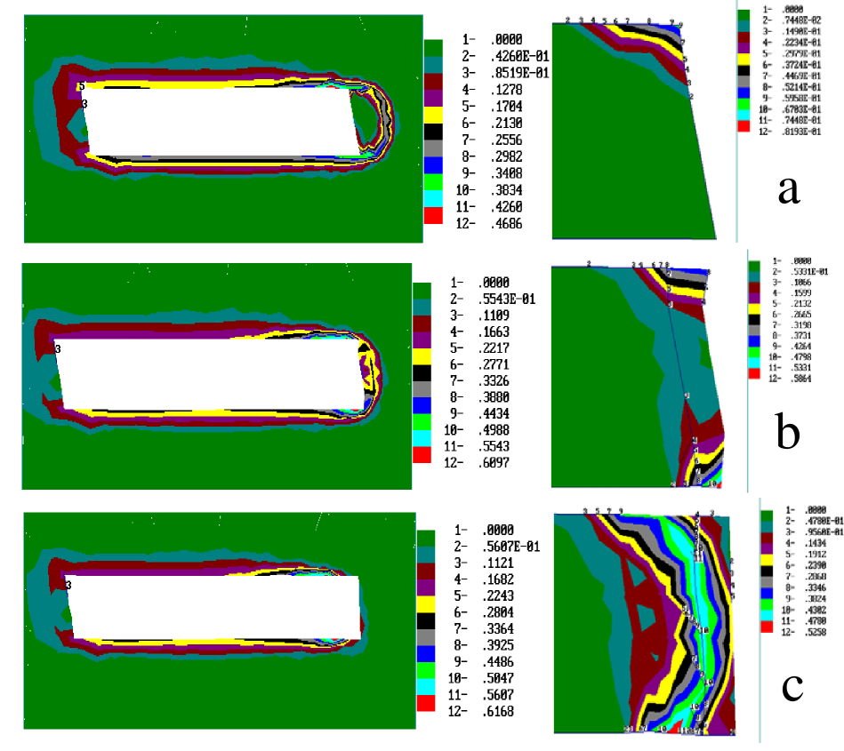
Interface velocity during lengthening as a function of the temperature and the interface location has been determined. The following conclusions were drawn in [266].
1. One of the key parts of the solution was a complete inheritance of the plastic strain of the austenite during its transformation to martensite. Thus, plastic strain tensor in the austenite was taken as an initial condition while integrating the flow rule in the transforming material. This led to the very heterogeneous and unexpected strain fields in the austenite and martensite and their nonmonotonous change during the PT process, see Fig. 19. The transformation deformation gradient was quite modest and the yield strength of the martensite was more than 3 times larger than that of the austenite (see Eq. (139)). Still, the plastic shear strain at some points of the martensite reaches 0.6 in the direction of the transformation shear and, after an elastic stage, changes the sign and increases by 0.4 in the opposite direction. The edge geometry of the propagating interface evolves counterintuitively (Fig. 19): the expected transformation shear strain profile changes to a wave-like contour with reverse shears near the corners, and then to almost straight vertical line. The plastic shear jumps by 0.9 across a phase interface.
2. These results shed a light on why the plastic deformation is localized in the much stronger martensite rather than in the weaker austenite. After nucleation, large plastic deformations are caused by the transformation strain near the interface mostly in the austenite. This plastic strain field is inherited by the growing martensite, causing, along with the transformation strain, significant internal stresses, which are relaxed via additional plastic flow (TRIP) in the martensite. After some growth increment, plastic deformations in the austenite are much smaller (see Fig. 19 (c)) because of small resultant shape change of the martensitic edge (see Fig. 19 (c)). Such a complex strain variation in martensite changes significantly the driving force for the interface propagation and athermal resistance .
3. After martensite nucleation and during increase in the lath length by 10 %, the transformation work decreases from MPa down to MPa and the contribution to due to the dislocation forest hardening grows from zero to MPa (compare to for the interfacial friction due to solute hardening). As a result, the net thermodynamic driving force for the interface propagation is getting negative, interface stops, and lath martensite is formed rather than the plate. It is also found that quite high internal shear stresses in the surrounding austenite may cause autocatalytic nucleation of new martensitic laths with the same or opposite transformation shear, which may coalesce, forming fine multi-lath structure.
The reduction of the yield strength of the austenite increases the plastic deformation and the propensity to formation of the lath. In particular, this happens for steels with high martensitic temperature, which leads to the reduction in the yield strength. Thus, the microstructure and mechanical properties of steels can be tailored by controlling the yield strength of austenite by alloying or preliminary plastic deformation.
4. A free surface does not essentially change the thermodynamic driving force for the PT until distance between the phase interface and surface is getting smaller than . After this, the transformation work grows and the Odqvist parameter and corresponding reduce abruptly. If not stopped before this position, the phase interface accelerates and reaches the surface. The edge interface contour passes via a wave-like shape, but ends with a shape produced by a transformation shear slightly modified by plastic accommodation, producing an asymmetric ’tent-shaped’ profile.
5. Obtained results allow one to understand the relationship between thermally activated kinetics for a single interface and athermal kinetics for a sample. For athermal nucleation postulated for martensite (see [369, 371, 372, 373]), this transition is related to the interface arrest due to reduction in and increase in independent of the interface kinetics for nonzero velocity.
Recent developments of modeling of dislocated lath martensite in steel can be found in [380].
16 Phase field approach to the interaction between plasticity and phase transformations
Thanks to the recent progress in nanotechnology and nanoscience, PT and plastic deformations are investigated in various nanoobjects: wires, fibers, films, multilayered systems, and particles. This encourages research on the coupled PT and discrete dislocation plasticity at the nanoscale. Thus, phase nucleation takes place at different dislocation configurations. Generally, nucleation always occurs in nanoscale volumes, even for bulk specimens. Loss of coherency of phase interface occurs via the dislocation nucleation and motion. Dislocations also produce athermal resistance to the interface motion. PFA is an ideal continuum method to address all of these problems.
PFA utilizes the concept of the order parameters, which describe the crystal lattice instabilities: for PT between the A and martensitic variants Mi and , which describes variation of the magnitude of the Burgers vector in the slip system from zero for perfect crystal to an integer number of dislocations.
The free energy has the number of the minima in the space of the order parameters and (separated by energy barriers) equal to the number of phases and variants, as well as the number of complete dislocations in the system. Besides, the free energy depends on the gradients of the order parameters that are localized in the finite-width interface and dislocation core regions. The gradient energy, together with local energy barriers between phases and dislocations, penalizes the interface and dislocation core energies. The solution of the thermodynamically consistent Ginzburg-Landau evolution equations for the order parameters describes in a continuous way the evolution of multiphase and dislocation microstructures. There is no need to satisfy jump conditions at the interfaces and to track motion of interfaces and dislocations. Characteristic solutions for the Ginzburg-Landau equations are evolving phase interfaces that have a finite width and divide multiple phases, and dislocation cores with a sharp but continuous variation of the Burgers vector, which separate sheared and non-sheared parts of a crystals.
In the previous PFAs on PTs and dislocation evolution [188, 315, 446, 9, 449, 448, 449, 161, 214, 208], these were the only constraints for choosing the free energy. Several other important conditions have been formulated in [290, 291] and then in [299] for PTs and in [292, 268, 272] for dislocations.
16.1 PFA to martensitic phase transformations
PFA is widely used for modeling martensitic PTs and evolution of corresponding microstructure, see [188, 315, 273, 446, 9] and the reviews [54, 328, 447]. We will concentrate on the approach with the order parameters representing internal variables that are related to the transformation strain or any other material properties [188, 273, 446, 9, 63, 401, 402, 54] because for the total strain-related order parameters [315, 396, 98, 388, 99, 18, 176, 439] we are unable to meet all the desired conditions. It is convenient to accept that in and in . The main requirements were introduced in [290, 291] for the description of the typical features of stress-strain curves, which are conceptually consistent with experimental results for shape memory alloys, steels, and some ceramics, and for the possibility to incorporate all thermomechanical properties of all involved phases. They were further developed in [282] for the temperature-induced PTs. These are the requirements:
(a) All material properties (transformation strain tensor, elastic moduli of any rank, thermal expansion tensor, etc.) that follow from the thermodynamic equilibrium conditions for homogeneous phases should be equal to the corresponding values for A and Mi. Stress hysteresis should be controllable—in particular, constant or weakly temperature-dependent.
Any material property can be interpolated between phases P0 and P1 in the form
| (146) |
where and are the property of P0 and P1, respectively, and is the interpolation function to be found. Requirement (a) leads to the following conditions for :
| (147) |
If Eq.(147) is not satisfied, then the thermodynamic equilibrium values of the order paramter will depend on the temperature and stress tensor. Substituting in Eq.(146) will lead to the artificial temperature- and stress-dependence of the property , and one could not restore the properties and for bulk phases P0 and P1.
(b) The PT criteria that are derived from the formulated crystal lattice instability conditions for the homogeneous and defect-free phases should have a desired form in terms of the stress tensor. This requirement was significantly elaborated in [299, 12] for satisfaction of the lattice instability conditions under general stress tensor obtained from the atomistic simulations [298, 464].
(c) All properties of A and Mi could be included in the thermodynamic potential and transformation strain.
While these requirements look quite natural, they were not satisfied in any theory for martensitic PTs prior to works by [290, 291, 292], where the PFA that meets these requirements was developed.
The large strain theory that meets these conditions was developed in [293, 289, 253, 300, 299, 12]. The theories that satisfy the above conditions were applied for FEM solutions of various static [273, 274] and dynamic [168, 64] problems at small strains, as well as at large strains in [289, 226, 12, 14].
16.2 Multivariant martensitic phase transformations and transformations in multiphase materials
16.2.1 Twinning and transformations between martensitic variants
Multivariant martensitic PTs are treated in most of the works within elasticity theory, see [188, 315, 273, 446, 9, 401, 402, 54, 328, 447, 274, 289, 226, 299, 12]. In particular, these approaches are applicable to the SMA. Since for most martensite lattices, some martensitic variants are in twin relationships to each other, transformation between them can be considered as twinning. However, twinning is also a mechanism of plastic deformation in general and represents a lattice-invariant shear producing invariant plane strain in martensite, in particular. That is why we shortly review the description of twinning and variant-variant transformations.
PFA for twinning that satisfies the above conditions (a)-(c) was developed in [290, 291, 292] for small strains and in [293, 253, 69, 70] for large strains. However, the main problem is in the description of variant-variant transformations. Since this problem is a particular case of a more general problem of multiphase PFA [415, 416, 123, 363, 31, 349, 350, 201, 422, 423, 424], which in most cases does not include mechanics and is devoted to grain structure evolution, we will include multiphase PFA in the discussion as well. A critical analysis of the multiphase PFA to PTs was presented, with further developments, in [424, 301, 282, 21].
16.2.2 Phase field models with Cartesian order parameters


In the first and most popular PFA presented in [188, 446, 9, 401, 402, 54], order parameters for martensitic variants were introduced, and each PT was described by a single order parameter (Fig. 20(b)). Then the analytical solution for an - interface allows one to perform a calibration of the width, energy, and mobility of an - interface. However, transformations occur along some curvilinear line in the - plane described by two order parameters (Fig. 20(b)) that depends in some uncontrolled way on the temperature and stress tensor. An analytical solution for an - interface cannot be found. The numerically determined energy, width, and mobility of - interfaces depend on the temperature and stress tensor in some uncontrollable way and cannot be calibrated by experiment. Since these theories also do not meet the requirements (a)-(c), even for the equilibrium order parameter is not but depends on the temperature and stress tensor. Because of this, it is difficult to obtain the thermodynamic - transformation criteria from the lattice instability conditions, and it is impossible to make them look like the criteria for twinning.
Theories that satisfy conditions (a)-(c) do not have problems with for and the thermodynamic - transformation criteria, but still transformations occur along some curvilinear line in the - plane, an analytical solution for - interface cannot be found, and the energy, width, and mobility of - interfaces cannot be calibrated by experiment.
16.2.3 Phase field theory with hyperspherical and polar order parameters
This problem was already recognized in [292], where an alternative PFA based on hyperspherical order parameters was developed (see Figs. 20(d)). In this and more advanced theory in [294] the radial order parameter describes PTs and angles characterizing the direction of the radius-vector describe PTs along the hypersphere . The angles meet a nonlinear constraint . Each transformation represents a quarter of a circle and is described by a single angular order parameter. Then the analytical solutions for all exist, and all interface widths, energies, and mobilities can be calibrated. While the desired crystal lattice instability conditions in terms of the hyperspherical order parameters were proved in [292], a flaw in this proof was found in [294], where also the nonlinear constraint was substituted by a linear constraint. This, however, also does not resolve the problem, see [301, 282]. No issues have remained only for two variants or three phases, the polar coordinates with a radial and single angular order parameters (Figs. 20(c)), without a constraint. In [277, 353, 351], such a model was developed and applied to PTs between two solid phases and melt, in particular, for solid-solid PT via intermediate (virtual) melt (see also Section 12).
16.2.4 Multiphase phase field approach utilizing linear constraint
In this approach the order parameters may be interpreted as the volume fraction of phases because they satisfy a constraint , see Fig. 20(a) and [415, 416, 123, 363, 31, 349, 350, 201, 422, 423, 424]. These approaches were mostly applied to solidification/melting and grain growth without coupling to mechanics; some applications involving stresses are presented in [414, 398]. The imposed constraint does not guarantee that each of the PTs occurs along straight lines connecting and variants (phases), which is necessary for avoiding a third (if spurious) phase between two others and description of a PT with a single order parameter. For three phases, this was accomplished in [117, 118] with some restriction on the kinetic coefficients. It was not evident how to extend the model for more phases. Also, since the appearance of a third phase is observed in some experiments (see [260, 249, 261, 281] and Section 12), an advanced model should be able to control this process. Subsequent analysis and improvement of the multiphase models was performed in Ref. [31, 424, 282, 21]. However, none of the PFAs with the above constraint properly described the lattice instability criteria.
16.2.5 Multiphase phase field approaches with penalizing functions
The models in [301, 282] deal with the Cartesian order parameters , without constraint but with the energy penalizing term that controls deviation from the straight lines connecting each and variant or two phases (see Fig. 20(e)). With the large (theoretically infinite) penalizing term, the path between two phases is the straight line that can be described by a single order parameter, an analytical solution for the propagating interface exists, and the interface energy, width, and mobility can be calibrated. No third phase is involved for the given case. At the same time, with the relatively small penalizing term, the third phase may exist within an interface, and the transformation path is curved (Fig. 20(e)). While this model is more advanced, flexible, and consistent than the previous, some problems have been found and were overcome in [21]. The main difference in [21] is that the PTs are described by a separate order parameter and other order parameters describe the martensitic variants within the plane (Fig. 20(f) and (g)). The transformation path within this plane is controlled with the penalizing term similar to that in [301, 282]. In addition, all multiphase junctions are penalized. Using separate order parameters for the and variant-variant PTs makes this theory much more flexible and removes contradictions found in [301, 282]. It was also developed for large strains and included interfacial stresses. Numerical algorithms and FEM solutions for this model were presented in [23].
A reaction pathway approach for reconstructive PTs was developed in [80, 81, 437]. Components of the transformation deformation gradient are used as order parameters instead of . Reverse PT may occur not only back to the initial A lattice, but to crystallographically equivalent variants A’ of the parent phase, obtained by rotation matrices in the point group of the A lattice. Each variant A’ can be transformed to multiple crystallographically equivalent variants of M’, and so on. Thus, a much larger number of variants (more than a hundred) is considered than in traditional theories for martensitic PTs described above. Gradient energy is dropped, making the theory and interface energy dependent on the mesh. This is justifiable for microscale theories (see Section 16.2.6), but questionable for nanoscale theories.
16.2.6 Microscale phase field models
The volume fraction of different phases as order parameters were utilized for martensitic PTs, e.g. in [267, 167, 222, 428, 414, 427, 355, 398, 91, 259, 92]. The simple mixture rule was used, all the interpolation functions are linear in volume fractions of phases, , and an energy barrier for PTs between phases and is . Such models are applicable for microscale simulations, when the interface width is either artificially increased from its actual size of a few nanometers by several orders of magnitude or processes in the interfaces are not important. In contrast to the nanoscale, the requirements for the first derivative of the interpolation functions in Eq. (147) are not mandatory and not satisfied.
16.3 PFA to dislocations
PFA to dislocations has many points borrowed from the PFA to martensitic PT in [188, 446]; it is widely utilized for simulation of plastic deformations in materials [448, 449, 452, 161, 162, 189, 214, 208, 163, 165, 164, 221, 27]. Plastic strain is used instead of transformation strain, which has a similar expression to crystal plasticity: summation of simple shears along all slip systems, with each shear represented by the dyadic product of the Burgers vector and normal to the slip planes. The order parameters for each slip system describe the magnitude of the Burgers vector. Small strain approximation along with Hooke’s law are utilized. Spectral methods have been applied for the numerical solution of Ginzburg-Landau equations for the order parameters and for the elasticity theory (the Khachaturyan microelasticity theory, see [448, 449, 450, 161, 162, 391]).
At the same time, these approaches inherited the drawbacks of the PFA for martensitic PTs, as well as some additional drawbacks. Some of them were resolved in [292, 268, 272]. In particular, thermodynamic equilibrium and crystal lattice instability conditions for homogeneous stress-strain states have been formulated and the thermodynamic potential and the interpolation function for the Burgers vector were designed to meet these constrains. This allowed us to ensure that the magnitude of the thermodynamically equilibrium Burgers vector is stress-independent and the artificial dissipation does not take place in the course of elastic straining; the desired crystal lattice instability conditions and a resolved shear stress - order parameter dependence are reproduced, all in contrast to previous theories. Besides, PFA in [272] is developed for large strain using the multiplicative decomposition of the deformation gradient into elastic and plastic contributions. Instead of interpolating the plastic strain tensor versus order parameters in the small-strain approaches, the relation for the plastic contribution to the velocity gradient versus the rate of the order parameters is postulated in the spirit of crystal plasticity. The height of a dislocation in [268, 272] has been defined by constitutive equations rather than by computational mesh in the published theories. Some simplified equations are presented in Box 11. A comparison with previous approaches is presented in [272].
One of the main ingredients of any phase field approach to dislocations is periodic crystalline energy , which is also called the generalized stacking fault energy or -surface. It represents an excess energy per unit area for any relative displacement of one part of a crystal with respect to another along the slip plane and direction. This energy has multiple zero-value minima corresponding to displacing a periodic lattice into a geometrically equivalent state, which determines the Burgers vectors of complete dislocations. We chose the simplest expression for that satisfies this condition. Partial dislocations and dislocation reactions are included in [403, 452, 47, 164, 341, 457]. Their consideration is based on the approximation of the more complex 2D energy landscape with additional intermediate minima, which is obtained using molecular static or first principle simulations. An alternative approach to dislocations based on the energy landscape in the total strain space is presented in [124, 15, 8].
Conditions on the interpolation functions imposed in [272] were not applied in the above papers, which should lead to stress-dependent equilibrium Burgers vectors and some undesirable features in the stress-strain curves.
16.4 PFA to the interaction of phase transformation and dislocations
Nucleation of M on dislocations using PFA to PT was studied analytically by [33, 207] and numerically by [388, 447, 326, 325, 467, 466, 196, 13]. Stationary dislocations were introduced using their analytical stress field or transformation shear. In [458, 459, 442], dislocations are introduced by preliminary plastic deformation, which did not evolve during PTs. Precipitates as nucleation cites were also included, and results showed low-hysteresis behavior of some SMAs, which was observed in experiments in [158].
In [214] dislocations are located at and move together with a phase interface and do not need separate phase-field equations. In reality, dislocations may move away from the phase interface into any of the phases, and they become inherited by growing phases, see, e.g., [270, 183, 184].
A continuum dislocation theory is coupled with the PFA for martensitic PT in [131, 132, 215]. In [215] the plastic sliding was allowed in A only and dislocations inherited by martensite retained the same eigen strain. Finite-strain crystal plasticity is combined with the PFA for martensitic PTs in [377], allowing slip in A only. It is applied to SMA. In [314], a similar approach is applied to twinning rather than to PTs.
In [140, 324, 462, 74, 460, 461, 76, 68, 67] the PFA to martensitic PTs is combined with the classical isotropic plasticity and applied to the growth of martensite. All the above approaches to the interaction between PTs and plasticity were for small strains. A reaction pathway approach for reconstructive PTs developed in [80, 81, 437] for large strain was supplemented by the elasoplastic or viscoplastic models in [81, 438] and applied for studying PTs and plastic flow in iron under static and shock loading.
Description of martensitic PTs in [19] is based on the combination of quasi-convexification of the nonconvex energy and classical von Mises-type plasticity. Micromechanical multiscale formulation and FEM solutions of some problems on interaction between PT and plasticity are described in [432, 209]. The nucleation and expansion of an elliptic martensitic inclusions with the prescribed aspect ratio combined with discrete dislocation evolution were analyzed in [404].
It should be noted that a conceptual problem exists in combining PFA to PTs with the theory of continuously distributed dislocations and especially with phenomenological plasticity. Indeed, the spatial scale of the problem on PT is determined by the interface width, which is on the order of 1 nm. The width of a martensitic variant is a few to 10 nm. The averaged distance between dislocations with as the dislocation density. For annealed materials , i.e., . For severe plastically deformed materials , i.e., . Continuum formulation requires at least several dislocations in each direction in the representative volume, i.e., it is applicable at the scale from two to five orders of magnitude greater than the phase interface width. That means that a nanoscale PFA to PT is consistent with discrete dislocation theories only. It is clear that any way to include plasticity and corresponding stress relaxation is more realistic than elastic formulation; but it should not be treated as a consistent theory.
At the same time, continuum plasticity can be coupled to the microscale PFA, where interface width is much broader or is not considered as a physical parameter, see e.g., [267, 169, 90, 259, 92]. An important point in these works is that martensitic variants are not spatially resolved and are described in terms of their volume fractions as internal variables. Another important feature in Ref. [259, 92] is that it includes a continuum description of dislocations along discrete slip planes, which allows reproduction of strong stress concentrators at the tip of the dislocation pileups that leads to the martensite nucleation, similar to the nanoscale approaches with discrete dislocations in [270, 183, 184]
It is important to note that in [131, 132] significant dislocation density was found within interfaces between martensitic variants. This is contradictory, because the variant-variant interface is an invariant-plane interface, which should not generate elastic stresses. It is found in [22, 21] that despite how the sharp variant-variant interface does not generate stresses, its finite-width counterpart within PFA does possess significant elastic stresses, which may lead to dislocations within an interface.
In [268], a simplified version of PFA for the interactions between martensitic PT and discrete dislocations (without presenting detailed equations) was applied to the solution of problems on nucleation and propagation of misfit dislocations along the interface and their effect on the athermal interface friction (see Section 11.6). For the stationary solution, both martensite and dislocations disappeared, illustrating reversible plasticity.
A simplified system of equations for the coupled evolution of dislocation and a single martensitic variant was suggested in [269, 270], however, without strict derivations. It was applied to various FEM solutions including revealing scale-dependent athermal semicoherent interface friction for direct and reverse PTs (see Section 11.6 and Fig. 12), reduction in PT pressure by up to an order of magnitude due to the dislocation pileup generated by shear strain (see Fig. 22), inheriting dislocations by a propagating phase interface, and the nucleation of dislocations by a growing martensitic plate, which leads to the plate arrest.
16.5 Complete system of the phase-field equations for the interaction between phase transformation and discrete dislocations
1. Kinematics
I. Finite strains
1.1. Multiplicative decomposition of the deformation gradient
| (148) |
1.2. Jacobian determinants
| (149) |
where (), (), (), and () are the elemental volumes (mass densities) in the reference , transformed , plastically deformed , and the actual () configurations, respectively.
1.3. Symmetric transformation deformation gradient
| (150) |
where is the transformation strain of a complete M variant and is the order parameter that describes PT from A () to M ().
1.4. Plastic part of the velocity gradient in the reference configuration
| (151) | |||
where is the Burgers vector of a dislocation in the slip system, is the unit normal to the slip plane; is the plastic shear produced by a single dislocation in a dislocation band with the height , ; is the order parameter for a dislocation in the slip system; and and is the integer part (defining number of dislocations in a dislocation band) and fractional part of .
II. Small strains
| (152) |
where is the displacement; designates the gradient in the ; subscript designates symmetrization; and are the small strain and rotations, respectively; and subscripts , , and are for elastic, transformational, and plastic parts, respectively.
2. Helmholtz free energy per unit mass
| (153) |
2.1. Elastic energy
| (154) |
where is the elastic Lagrangian strain tensor and is the fourth-rank tensor of elastic moduli, which are assumed here as the same for both phases. Note that the definition of in Eqs. (153) and (154) differs from that in Box 9.
2.2. Thermal energy
| (155) |
where and are the differences between the thermal part of the free energy and entropy for M and A, respectively; is the magnitude of the double-well barrier between A and M at phase equilibirum; is the thermodynamic equilibrium temperature for stress-free A and M; is a parameter; and is the critical temperature at which stress-free A loses its thermodynamic stability.
2.3. Periodic in space crystalline energy
| (156) |
where and are the magnitudes of the multi-well crystalline energy in A and M, respectively, that define the critical shear stress for barrierless nucleation of a dislocation (i.e., the theoretical shear strength); is the coordinate normal to the slip plane; and is the width of the thin layer between dislocation bands.
2.4. Energy of interaction of dislocation cores belonging to different slip systems
| (157) |
where and are the corresponding magnitudes for A and M, respectively.
2.5. Gradient energies for PTs and dislocations
| (158) | |||
| (159) |
where is the coefficient of the gradient energy for PT; and are the coefficient of the gradient energy for dislocations in A and M, respectively; is the ratio of the coefficients for the gradient energy normal to and along the slip plane; and superscripts and stand for the directions along and the normal to the slip plane, respectively.
3. First Piola-Kirchhoff and Cauchy stress tensor
I. Finite strains
| (160) |
| (161) |
II. Small strains and linear elasticity
| (162) |
4. Ginzburg–Landau equations
4.1. Compact form in the at finite strains
| (163) |
where , and are the kinetic coefficients for PT and dislocations in A and M, respectively; and are the thermodynamic dissipative forces work-conjugate to and , respectively; and is the resolved shear stress for a dislocation.
4.2. Detailed form at finite strains
| (164) |
| (165) |
4.3. Small strains, linear elasticity
| (166) |
The Ginzburg-Landau equation for dislocations for small distortions looks like Eq.(165) with the simplified expression for .
In [271] a large-strain and thermodynamically consistent PFA for combined discrete dislocations and multivariant martensitic PTs is suggested. It synergistically combined and extended the most mechanically advanced PFA to martensitic PT in terms of the order parameters [253] and dislocations in terms of the order parameters [268, 272]. Details for PFA to PT and dislocations separately can be found in these papers. For compactness and simplicity, we present in Box 9 the particular case of a complete system of equations from [182] with the following simplifications in comparison with the general theory in [271].
(a) Slip systems of A and M, transformed back to A, coincide, i.e., all slip systems are inherited during the direct and reverse PTs. This is the case, e.g., for PTs between b.c.c. and body centric tetragonal (b.c.t.) crystal lattices as well as for PTs between f.c.c and f.c.t. lattices.
(b) We consider a single M variant.
(c) Surface energy is independent of phase and dislocations, which results in the simplest zero-flux boundary conditions for and .
Box 11 also contains simplified equations for infinitesimal strains. The key problem was to justify the best kinematic decomposition. Several quite natural and logical options of multiplicative decomposition of the deformation gradient , e.g., , with and for the plastic deformation gradient in A and M, were rejected due to some undesired features. The thought experiments considered cyclic A-M PTs and plastic deformation of A and M after PTs, with focus on the inheritance and evolution of dislocations during and after PTs, along the inherited slip systems that do not belong to the traditional ones for the product crystal lattice.
The multiplicative decomposition (148) of the deformation gradient into elastic, transformational, and plastic contributions (exactly in this order) is justified (Fig. 5). Eq. (149) defines the corresponding Jacobian determinant describing ratios of elemental volumes in different configurations. A symmetric transformation deformation gradient is interpolated in terms of the order parameter describing PT by Eq. (150), while more advanced expressions justified in [299, 21] are currently available.
Generally, the plastic part of the velocity gradient includes four different mechanisms: (a) dislocation evolution in M along the natural slip systems of M and (b) slip systems of A inherited during PT; (c) dislocation evolution in A along the natural slip systems of A and (d) slip systems of M inherited during reverse PT. Equations for transformation of the parameters of the slip systems inherited by the crystal lattices during PT are presented in Fig. 21 and caption.
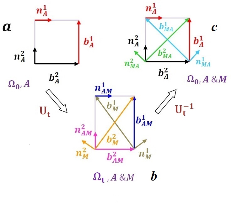
It is proved that the definition of (a) in M expressed as a combination of plastic shear rates along the slip system of M and (b) in M transformed back to A expressed as a combination of plastic shear rates along the slip system of M back-transformed to A are equivalent. This result leads to the description of of M in the crystal lattice of A with the same expression as in the crystal lattice of M, however, with transformed-back crystallographic parameters of the slip systems of M to the A. This also led to the additive combination of for all four mechanisms using crystal lattice of the A. The for all four mechanisms is expressed in the crystal lattice of the A using slip systems of A and transformed-back slip systems of M, and just two corresponding types of the order parameters. This is a noncontradictory and economic decomposition, in contrast to, e.g., a multiplicative decomposition of into in the M and A. When the slip systems of A and transformed-back slip systems of M coincide, Eq. (151) for utilizes just one type of the order parameters, like in the PFA for dislocation without PT by [272].
The Helmholtz free energy per unit mass consists of elastic, thermal, and periodic in space crystalline energies, the energy of interaction of dislocation cores belonging to different slip systems, and gradient energies for PT and dislocations, see Eqs. (153)-(158). Utilization of the thermodynamic laws results in the elasticity rule (Eqs. (160)-(162)) and expressions for the driving forces for PT and dislocation evolution (16.5). The Ginzburg-Landau equations are obtained as the linear relationships between the thermodynamic driving forces and work-conjugate rates and are expressed in a compact and detailed form in Eqs. (16.5)-(166).
Various types of coupling between PT and dislocations are included in the theory. The nonlinear kinematic decomposition (148) already contains such a coupling resulting in the presence of in the transformation work and in the definition of the resolved shear stresses . For infinitesimal strains this type of coupling disappears. All material parameters for dislocations depend on since they have different values in A and M. Due to such a dependence, additional terms in the Ginzburg-Landau equations for PTs appear due to the change in dislocation structure and properties. Also, dislocations are inherited during PT and they may further evolve along the nontraditional slip systems if corresponding critical shear strength is reached. In addition, one of the strongest interactions between PT and dislocations occurs through their eigen-stress fields, which is determined by a solution of the continuum mechanical boundary-value problem. Application of the developed theory to the solution of some important material problems is presented in [182, 183, 184].
17 Phase transformations and chemical reactions induced by plastic shear under high pressure
The main experimental phenomena related to the PTs and CRs under pressure and shear are reviewed in [41, 42, 474, 475, 28, 87, 246, 252]. Theoretical treatment was initiated in [247, 246]. The current four-scale theory (from atomistic to macroscale behavior of a sample) is recently reviewed in [252]. To minimize repetitions, this Section will be short.
17.1 Main phenomena
One of the most impressive effects of plastic deformation on the PTs and CRs is observed in experiments on high-pressure torsion under constant applied force. Initially, this work was performed in metallic or ceramic rotational Bridgman anvils (see [41, 42] for PTs and [474, 475, 61, 88, 89] for CR), which are currently used for grain refinement and producing nanograined materials [434, 436, 435, 87, 477]. Currently, much more precise in-situ experiments are performed with the rotational diamond anvil cell (RDAC) [28, 186, 122], see inset in Fig. 24. Among numerous phenomena that are observed in these experiments (see [41, 42, 28, 247, 246, 252]), we enumerate just three the most important ones. Thus, plastic shear under high pressure:
(a) leads to the formation of new phases and reaction products that were not be produced without shear [41, 42, 28, 87, 29, 474, 476, 302, 246, 252];
(b) reduces the transformation pressure by a factor of 3 to 10 for some PTs [41, 42, 28, 87, 285, 186] and chemical reactions [474, 476], and even by a factor of 100 for the PT from graphite to diamond [122], and
We will discuss the most advanced results on characterization and general properties of strain-induced PTs in RDAC. The in situ quantitative synchrotron X-ray diffraction investigation of plastic strain-induced PT in Zr was performed in [375]. The most consistent results were obtained for strongly plastically predeformed Zr, when strain hardening saturates and material hardness and yield strength and microstructure do not evolve with further plastic deformation [236, 87, 435, 305]. Polycrystalline materials for this case behave like perfectly plastic and isotropic with plastic strain history independent surface of perfect plasticity [236]. We assumed that since the plasticity theory for such large strains is significantly simplified, the kinetics of strain-induced PTs will be more tractable as well, and this is the best and repeatable initial state to start with. This was the case in experiments. Working part of sample looks like a coin, with diameter of (diamond cullet) and thickness reducing from down to and less, depending on the applied force and the rotation angle of an anvil. Distributions of pressure in each phase and in the mixture, and volume fraction of -Zr along the radius, all averaged over the sample thickness, as well as thickness profile were measured using synchrotron X-ray diffraction and X-ray absorption. The simplified version of the strain-controlled kinetic equation derived in [247, 246] (which is a particular case of Eq. (123)) is
| (167) |
Here, is the yield strength of -th phase; and are the minimum pressure at which the direct strain-induced PT may occur and maximum pressure at which the reverse strain-induced PT proceeds, respectively, is the Heaviside step function used to impose criteria for the direct () and reverse () strain-induced PTs; and are the pressures for the direct and reverse PTs under hydrostatic loading; all remaining symbols are material parameters. Eq.(167) includes the possibility of direct and reverse PTs and the different plastic strain in each phase due to different . For -Zr, the reversed strain-induced PT was not observed in [375], i.e., the second term in Eq.(167) disappears. Eq.(167) was confirmed experimentally and all material parameters were identified. In particular, the minimum pressure for the strain-induced PT, =1.2 GPa, is 4.5 times lower than under hydrostatic conditions and 3 times lower than the phase equilibrium pressure. The is found to be independent of the compression-shear straining path. This means that the strain-induced PTs under compression in DAC and torsion in RDAC do not fundamentally differ for Zr.
17.2 Atomistic studies
Molecular dynamics [298, 258] and first principle simulations [464] were performed for an ideal lattice. Under guidance of the analytical treatment of the martensitic PTs within PFA [253], they led to an explicit expression for the PT (i.e., lattice instability) condition for cubic - tetragonal Si ISi II transformations under action of all six components of the stress tensor. The strong effect of nonhydrostatic stresses was exhibited, in particular, in the following result: the pressure for Si ISi II PT under uniaxial compression was reduced by a factor of 20 in comparison with hydrostatic loading [464]. Stress-strain curves for different loadings were determined as well. A new phenomenon was predicted [258]: unique homogeneous and hysteresis-free first-order phase transformations for which each intermediate crystal lattice along the transformation path is in indifferent thermodynamic equilibrium and can be arrested. Elastic energy for Si I was analytically presented in terms of the fifth-degree polynomial of the Lagrangian strain in [51], for finite strains including lattice instability points.
Because of different effects of the stress tensor on the PT conditions for the direct and reverse PTs, these atomistic results led to essential generalization of the PFA in [299, 12]. This advanced theory was applied to the nucleation and growth of Si II at a single dislocation in [13], and the importance of the generalized PT criterion is demonstrated.
17.3 Nucleation and evolution of high-pressure phase at dislocation pileups
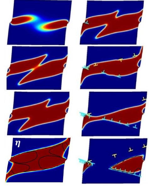
As the main nanoscale mechanism of drastic reduction in PT pressure in experiment due to plastic deformations, a strong concentrator of the all components of the stress tensor at the tip of dislocation pileup was suggested in [247, 246] and treated analytically. Much more precise results were obtained in [270, 182, 183, 184] using PFA approach to interaction between dislocations and PTs presented in Section 16.5 and [271]. Example of the solution for a bicrystal under compression and shear is presented in Fig. 22. Dislocation pileup located in the left grain (not shown) creates a strong concentrator of all components of the stress tensor in the right grain, which exceeds the crystal lattice instability limit and leads to a barrierless nucleation of a HPP. It is also important that the deviatoric stresses in the nanoscale defect-free regions are limited by the theoretical strength rather than the macroscopic yield strength and may be one to two orders of magnitude greater. All this increases the local driving force for PT, enabling drastic reduction of the applied pressure to initiate and run the PT. For the chosen parameters, the applied pressure is 3-20 times smaller than the PT pressure under hydrostatic conditions in the presence of a single dislocation and 2-12.5 times lower than the phase equilibrium pressure. The unique highly deviatoric stresses that cannot be achieved for the macroscopic sample may lead to new phases and phenomena. The stationary geometry of the HPP is determined by the thermodynamic equilibrium
| (168) |
either at point of the interfaces (Fig. 22) or in terms of the stress tensor averaged over the entire grain or polycrystal. In the local approach, stresses due to dislocations are included in ; if separated from the external stresses, they will reproduce an athermal threshold for interface motion due to interaction with dislocations (see also Section 11.4).
For larger scale, a scale-free PFA for the coupled evolution of multivariant martensitic microstructure and discrete dislocation bands was presented in [259, 92]. It includes a scale-free PFA for martensitic PTs [267, 167, 91]. Dislocation pileups or shear bands are introduced by the contact problem formulation, considering continuous sliding displacements (dislocations) along the discrete slip systems. This allows one to produce stress concentrators required for nucleation of the HPP, similar to the nanoscale approach described above. Scale-free model, while is much simpler than the nanoscale model, reproduces well all results obtained for nanoscale model for a bicrystal. Also, this model is applied in [259, 92] for FEM simulations of the strain-induced PTs in a polycrystal sample under compression and shear (Fig. 23). The phase equilibrium condition (168) in terms of local transformation work at the interface and transformation work averaged over the entire polycrystal was confirmed. Also, similar to the nanoscale model, we obtained for the scale-free model that stresses averaged over all martensitic and austenitic regions, as well as for the entire polycrystal are equal:
| (169) |
Note that result similar to Eq. (169) was obtained in [219] for traditional continuum plasticity and sharp interface rather than for the PFA and localized plasticity. Also, evolution of the volume fraction of HPP in each grain and in a sample, and averaged over the sample the volume fraction of HPP, each martensitic variant, pressure, and shear stress versus shear strain are determined in [259, 92]. All the obtained info is planned to be applied for derivation of more precise strain-controlled kinetic equation than Eq. (167), which is currently used.
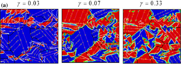
MD simulations in [52] on amorphization of Si I at the tip of the shuffle dislocation pileup against three different grain boundaries under shear confirms main the analytical [247, 246] and PFA [270, 182, 183, 184, 259, 92] results. Thus resolved shear stress for initiation of amorphization reduces from GPa for perfect crystal down to GPa for 8 dislocations in a pileup. At the same time, screw shuffle dislocations in Si I pass through all three grain boundaries (, , and ) and cannot pileup, and consequently affect a PT [53]. Atomistic mechanism of strain-induced nucleation of amorphous phase, different for different grain boundaries is elucidated. While grain boundary amorphous band propagates along the plane directly, for , and boundaries the stacking faults and an intermediate phase precede the formation of an amorphous band along the and planes, respectively.
MD simulations of the interactions of plasticity and PT under shock in iron bicrystals in [468] also confirms the reduction in PT pressure due to the effect of the grain boundary and dislocations induced by grain boundary and pre-existing dislocations. This work also gives important atomistic detail of the promotion of the PT and distinguishes between strain- and stress-induced PTs.
At the same time, in the MD studies of shock loading of a polycrystalline iron sample [190, 135, 136, 444] dislocation activity is suppressed by small grain size ( nm), or PT precedes plastic flow, and nucleation of the high-pressure phase is promoted by grain boundary and triple junctions.
The simultaneous occurrence of dislocation bursts [145] and amorphization in SI has been found in shock experiments [469, 470, 471]. In these works, both MD simulations and transmission electron microscopy offer that the stacking faults along planes and their intersections serve as nucleation sites for amorphization. For larger shock intensity, the amorphous band broadens and deviates from the plane toward the maximum-shear-stress plane. Shock-induced amorphization in SiC was studied in a similar way in [472]. Amorphization in without dislocations under uniaxial loading was studied with MD and experimentally in [318].
17.4 Macroscale theory and FEM modeling of strain-induced transformations
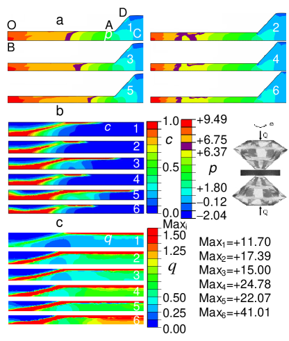
The main goal of a macroscopic modeling and simulations is to determine the evolution of the distributions of the components of the stress tensor, accumulated plastic strain, and the volume fraction of the HPP [295, 296, 100, 102] in a sample compressed in DAC and twisted in RDAC, see example in Fig. 24. The first results were obtained analytically in [247, 246] with many simplifications, but still some important conclusions were made. The first FEM results in [295, 296] were much more comprehensive, but still the material and contact friction models were simplified. The most advanced model for coupled large elastoplasticity and strain-induced PT under megabar pressure and corresponding FEM algorithms were developed and applied to study PT in BN under compression in DAC [100] and torsion in RDAC [102] within rhenium gasket. Finite-strain kinematics for a polycrystal included multiplicative decomposition of the deformation gradient into elastic and inelastic parts, and then inelastic deformation rate was additively decomposed into plastic and transformational parts, different from the multiplicative decomposition (148) for a single crystal. Murnaghan elasticity rule and pressure-dependent Prager-Drucker yield condition for each phase along with the simplest mixture rule were utilized. Kinetic Eq. (167) for strain-induced PT was implemented as well. Third- and fourth-degree anisotropic elastic energy were utilized for diamond [103, 305]. Combined Coulomb and plastic friction between sample, diamond, and gasket were considered. Without PTs, elastoplastic models were calibrated and verified by independent experiments for rhenium [103, 101, 104] and tungsten [305] up to 300 GPa and 400 GPa, respectively. Various experimental phenomena have been reproduced and explained, some have been predicted, methods of controlling PTs were suggested, and some possible misinterpretations of experimental results have been demonstrated, see [246, 252].
18 Scale transitions and phenomenological theories for interaction between phase transformation and plasticity
An averaged description of phase transformations in terms of the volume fraction of phases is presented in [227, 228, 385, 25, 60, 59] at small strain and in [228, 381] at large strain. An averaging procedure for PT with semicoherent interfaces at large strains is developed in [237]. A computational studies of martensite formation and averaging, including multicale approaches, can be found in [219, 121, 332, 331, 333, 405, 263, 432, 433, 209, 175]. Strain-induced PTs are described in [370, 418, 82]. Significant progress in the study of TRIP is presented in [113, 115, 60, 58, 368].
More detailed studies, e.g., [152, 174, 218, 24, 200, 330] demonstrate dependence of PT kinetics on strain/stress mode and path, texture, temperature, and strain rate; some of them include constitutive modeling. Simultaneous occurrence of stress-induced and plastic strain-induced PTs was modeled in [321, 107]. In the last paper, these two types of PTs are distinguished based on the transformation mechanism: for stress-induced PT -austenite transforms directly to -martensite, but for strain-induced PT these transformation occurs through appearance of bands of -martensite, and -martensite nucleates at intersection of these bands (alternatively, martensite may nucleate at intersection of twins [78]). An advanced version of elastoplastic self-consistent approach to the behavior of polycrystalline aggregate, initially developed in [431] was implemented.
Simulations of the interaction between PTs and plasticity, utilizing macroscscale constitutive equations can be found in [295, 296, 406, 322, 323, 45, 395]. Models and simulations for single crystals and dynamic loading can be found in [20, 105, 106]. Some theories and FEM approaches to strain-induced PTs coupled to large elastoplasticity under high pressure were analyzed in Section 17.4.
19 Fracture and interaction between fracture and phase transformation in inelastic materials
A general theory summarized in Boxes 1, 2, and 6-8 is applicable to fracture, including crack and void nucleation and growth [248, 244, 172]. Fracture is defined as a thermomechanical process of change in some region of tensile and shear elastic moduli and yield strength from their initial values to zero. This process cannot be arrested at a material point in the intermediate state. After complete fracture, the tensile stresses in the fracture region are zero. Formally, fracture here is considered as a particular case of a PT without transformation strain and a specific properties of the product phase (vacuum), which was coined in [248, 244] a generalized second-order PT. With such a definition, local driving force Eq. (37) for an isothermal fracture, neglected internal variables, and independent of free energy, reduces to
| (170) |
It is not clear where to get . In applications, it can be included in athermal friction or just neglected. But we will keep it for generality.
Similar to PTs, the developed approach is valid for an arbitrary inelastic material, because the constitutive equations were not used in the process of derivation. To illustrate the method, we consider analytical solutions to two simple problems.
19.1 Crack propagation in elastoplastic material

Equations for crack propagation in an elastic-perfectly-plastic material were derived in [248, 244] in a framework similar to the [86] framework for the plane stress. The localized plastic region (Fig. 25) ahead of the crack is subjected to cohesive stresses on the extended crack surfaces and ; is the fracture zone. The transforming volume before fracture , where is some intermediate value of the crack opening at the length and is the thickness of the sample.
Neglecting all the stresses and elastic strains but normal to the crack plane only and assuming that during the fracture process
| (171) |
we obtain that the work integral in Eq.(170) is zero. Evaluating elastic energy, we obtain
| (172) |
which is uniform in the fracture region and is independent of its geometry; thus, we have to use equations from Boxes 6-8. The thermodynamic fracture criterion and the principle of the minimum of transforming mass can be expressed as
| (173) |
The minimum value of is determined from the fracture criterion (173). Condition leads to , where is the interatomic distance in the direction of crack propagation. Then is the crack opening displacement between points and and the thermodynamic fracture criterion (173) can be transformed to the criterion of critical crack opening
| (174) |
In contrast to previous publications, the critical crack opening is defined in terms of known material parameters.
For the Dugdale model [389], where is the path independent -integral for the pathes that do not cross the plastic region. Then criterion (174) can be expressed in term of the critical value of -integral
| (175) |
Eq. (67) for transformation time can be expressed as a kinetic equation for a crack growth:
| (176) |
Eq.(176) can be easily transformed to the traditional Arrhenius equation formulated in [478] kinetic concept of strength based on experimental regularities, see also [57]. In our solution the crack propagates atom by atom, i.e., almost continuously, in contrast to the discrete finite crack advance in the model by [198]. The characteristic size in our model is the thickness .
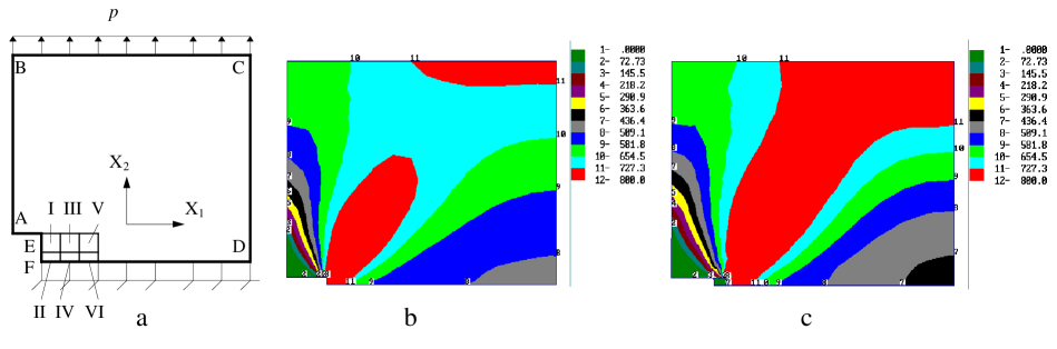
FEM study of ductile fracture in a sample with edge notch under tension (Fig. 26 a) based on the same theory is given in [172]. Six regions in a small rectangular near the edge notch was considered in different combinations as a possible fracture zone. The distribution of von Mises stress before fracture and after fracture in regions I-VI is shown in Figs. 26 b and c, respectively. After solving multiple elastoplastic problems with fracture in different regions (modeled as incremental reduction of elastic moduli down to zero), the mechanical part of the driving force was evaluated, and various scenarios were compared (Table 1).
For example, for fracture in narrow regions II, IV and VI, is larger and its growth is faster during the fracture propagation than for thick regions I, III and V. However, the resistance due to the surface energy for a thin layer is larger than for a thick layer. When fracture occurs simultaneously in regions II + IV or II + IV + VI rather than first in a small region II and then spreads through regions IV and VI, the is larger, i.e. it is thermodynamically more favorable scenario. However, the damaging volume grows by factors 2 and 3, respectively. Thus, the subsequent growth is more favorable kinetically, if the thermodynamic criterion is met.
At a relatively small surface energy, a void nucleation in region VI occurs instead of crack propagation. The mechanical driving force is significantly larger than for any damage scenarios. After pore nucleation fracture propagates from pore to notch. This corresponds to a well-accepted experimental result that the void nucleation and bridging ahead of the crack tip is an actual physical mechanism of ductile fracture.
An analytical approximation of the computational results for allowed us to analyze the application of macroscopic thermally activated kinetics from Boxes 5, 6, and 8. Below are the found typical cases in the determining two characteristic sizes of the fracture region: (a) from the principle of minimum of fracture time without any constraints; (b) from the thermodynamic fracture criterion; (c) as an interatomic distance, and (d) as the sample size. In some cases crack advance is finite; however, different from [198], the advance is determined from the extremum principle or the thermodynamic fracture criterion rather than being a chosen material parameter.
![[Uncaptioned image]](/html/2105.10932/assets/x31.png)
19.2 Interaction between fracture and phase transitions
Relatively large transformation strain induces high stresses, that may relax by crack and void nucleation and growth instead of plasticity, see examples in [156]. At the same time, a large stress concentrator at the crack tip may induce PT [419, 48], which may increase material toughness; this is the so-called transformation-toughening phenomenon.
To illustrate some types of interaction between fracture and PT in elastoplastic material, several model problems were solved in [172] for sample and loading shown in Fig. 26a. Obtained results are presented in Table 2. For fracture in region II, before PT and after PT in region I + II, due to stress relaxation caused by dilatational transformation strain. Fracture in region II + IV decreases the mechanical driving force for PT in region I down to MPa due to stress release and increases for PT in regions V and VI by moving stress concentrator closer.
Next, consider competition between PT and fracture for athermal (time-independent) kinetics, see Box 4. We compare four processes: PT region I + II or in I–IV, and fracture in region II or in region II + IV. Let each of these processes be thermodynamically admissible, i.e. the thermodynamic SC criterion (44) is met for the selected values of the surface energy and . One has to select which thermomechanical process will take place in reality, i.e., to choose the single solution among all possible ones. This is situation described in Section 6.6, i.e., the best unique solution is the stable one.
According to the extremum principle (51), which is the global SC criterion for the determination of the stable deformation process, for the prescribed normal stress the larger the normal displacement averaged over line BC is the more stable is the SC process. Based on Table 3, fracture in region II + IV should occur as the most stable SC process. If for fracture in region II + IV the thermodynamic fracture criterion (44) is not met, then PT in region I–IV should take place. For the case when PT in region I + II and fracture in region II are the only thermodynamically possible, the fracture will occur. Consequently, similar to PTs (see Section 14), in addition to the thermodynamic fracture and PT criteria (44), the global fracture and PT criteria (50) and (51) based on stability analysis should be applied for some cases.
For time-dependent kinetics we do not need additional global fracture and PT criteria for this case. Indeed, the principle of minimum of transformation time allows us to choose which process – PT or fracture – will occur in the shortest time. However, in the case of time-dependent kinetics of PT or fracture and time independent plasticity we may need the global criterion of SC again, because plastic flow without PT and fracture may be the most stable process.
![[Uncaptioned image]](/html/2105.10932/assets/x32.png)
![[Uncaptioned image]](/html/2105.10932/assets/x33.png)
One of the remaining problems is the mass balance for fractured material. In the energy methods of fracture mechanics the fractured region is removed. From physical point of view, fracture means that atoms are separated by the distance when their interaction is negligible. For such a formulation, the volume of the fracture region increases during the fracture process from zero to some value determined by a solution of a mechanical problem. For modes II and III, crack surfaces can be in contact.
Other problem is related to definition of fracture: which components of the elasticity tensor tend to zero and in which sequences? The stress state and thermodynamic driving force may depend on the chosen process.
19.3 Void nucleation in infinite elastoplastic sphere
Spherical void nucleation in an infinite elastic-perfectly-plastic sphere under a homogeneously distributed tensile stress was considered in [244] in small strain approximation. Fracture process was modelled by decreasing the bulk modulus in a small sphere with a radius from an initial value to zero accompanied by jump under isothermal conditions. The stress state for this problem was taken from [393]. Surface stresses were neglected. For an elastic material, the mean tensile stress inside the transforming zone is
| (177) |
where and are the elastic bulk compliance of undamaged material and during the fracture, , is the shear modulus of undamaged material. For a void after fracture , . After integration one obtains
| (178) |
where and are Young’s modulus and the Poisson ratio of the undamaged material.
For void nucleation in an elastoplastic material, during the increase in compliance , the material initially deforms elastically. Plastic deformation near the damaging region starts at determined from equation
| (179) |
According to [393], in the elastoplastic regime variation of stress is determined by equation
| (180) |
After manipulations, one obtains for elastoplastic regime
| (181) |
Since is independent of radius , we can use the same equations and conclusions like for PT in a spherical nucleus in Section 8. For macroscale thermally-activated kinetics, the principle of minimum mass results in condition and equation from Box 7 are applicable for the radius of the thermodynamically admissible void and the fracture time. One can also apply equations in Box 4 to described thermally activated void nucleation, like for PT in Section 8.
For an elastic sphere, the thermodynamic criterion for void nucleation was presented in [57]. It was obtained that the stress required for void nucleation reduces with the increasing void radius, i.e., nucleation of an infinite void needs the smallest . The same should be true for elastoplastic sphere. In contrast, our kinetic approach allows determination of the explicit void radius and nucleation time versus applied tensile stress.
Numerous papers are devoted to the void nucleation and growth due to diffusion of vacancies, Kirkendall effect, and chemical reaction, see e.g., [109, 311] and references herein.
Thermodynamic driving force for a void growing in elastoplastic material
19.4 Alternative approach to void nucleation
Completely different definition of the void nucleation due to fracture is accepted and used in [256]: it is a thermomechanical process of the growth of a cavity inside the solid from zero to some critical size due to atomic or molecular bond breaking. Applying our thermodynamic approach to such a definition, taking into that dissipation due to fracture only is independent of the volume under consideration, and considering sample infinitesimally larger than a void, it was obtained for the thermodynamic driving force
| (182) |
where is the traction vector in the solid at the variable void surface , and is the displacement vector and its normal component at the void surface, and is the mean curvature of the void surface. Thus, the thermodynamic driving force for the void nucleation (i.e., the dissipation due to fracture only) is localized at the void surface, is independent of plastic strain in solid, and represents the difference between work produced by external traction acting on the void surface and work produced by the Laplacian pressure . For a spherical void of a radius under axisymmetric normal tensile stress in solid at the void surface, Eq. (182) simplifies to
| (183) |
Here is the radius of the critical nucleus, which can be found from minimization of with respect to , or equivalently, from the mechanical equilibrium equation . Since for a subcritical nucleus , the thermodynamic driving force is negative, and determines the energy necessary for void nucleation, which is supplied by the thermal fluctuations. The large-strain solution to the perfectly plastic problem on expansion of a spherical cavity from zero size [154, 254] is
| (184) |
Here, and is the cavitation pressure, i.e., the possible maximum value of tensile pressure that solid can sustain for neglected surface energy. Utilizing for such a driving force a kinetic theory from Box 4, we obtain the explicit relationship between tensile stress for nanovoid nucleation vs. temperature:
| (185) |
In addition to fracture, void nucleation may also occur due to PT-related mechanisms [254, 255, 250, 257], namely due to direct sublimation (i.e., transformation of a critical volume of solid to gas), sublimation via virtual melting, and kinetic melting and evaporation of a stable liquid. Fig. 27 from [256] shows a complete temperature-tensile stress kinetic diagram for void nucleation due to different processes.
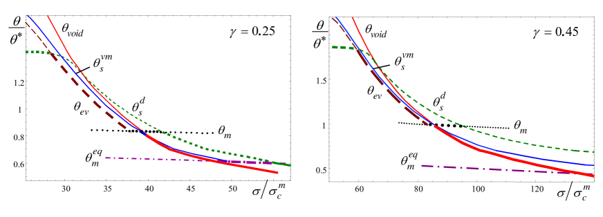
19.5 Phase field approach to fracture
It is clear from solutions in Section 19 that search for crack trajectory in elastoplastic materials based on the presented sharp interface theory and extremum principle is very computationally expensive. Similar to PT, PFA with finite-width interface is much more effective for this purpose. The PFA has been widely used for the simulation of fracture [7, 195, 153, 146, 147, 409, 211, 342, 36, 37, 32, 2, 85, 456] and damage [357, 358, 456, 440].
The order parameter in the majority of PFAs to fracture characterizes atomic bond breaking in a solid and separates a sample into the undamaged solid (), fully broken atomic bonds (), and the finite-width crack surface, in which the material is partially broken (). The evolution of the damage order parameter occurs mainly in the crack tip zone and is described as a solution of the corresponding Ginzburg-Landau equation. The Ginzburg-Landau equation coupled with mechanics, i.e. kinematics, constitutive rules, and equilibrium/motion equations, are used to obtain the evolution of the order parameter and stress-strain fields. All PFAs to fracture can be divided into two groups: with a double-well potential, like for PTs, and with a single-well potential.
PFAs with double-well potential. The first PFA for crack propagation utilizing the Ginzburg-Landau equation for PT was presented in [7] with the concentration of point defects as the order parameter. The coupled Ginzburg-Landau and elastodynamic equations were utilized for finding the evolution of the order parameter and displacement fields for mode I crack propagation. The KKL (Karma-Kessler-Levine) PFA for mode III of fracture [195] was similar to the conventional PFA to dendritic solidification, i.e. to PT. The double-well energy barrier between the gaseous and the solid states mimiced the fracture energy. This model overcame some limitations in [7], which could not completely release the nonphysical bulk stresses. The KKL model [195] has been generalized to modes I and II of crack propagation in [153] and for description of quasi-static crack growth paths in elastically anisotropic materials in [146, 147]. In [147], the double-well term was substituted with the critical elastic energy and 1D analytical solution was presented. Some drawbacks of the KKL model was discussed in [306] by analyzing the stress-strain curves for the homogenous states. Some other PFA approaches with double-well term were developed in [409, 410, 178] and for modeling of damage in [357, 358].
The PFAs with a double-well barrier treat fracture as a solid-gas transformation while it is an atomic bond breaking; they lead to crack widening and lateral expansion during its propagation, see [307, 37].
PFAs with single-well potential are not related to PTs, see [119, 36, 4, 211, 342, 37, 32, 2, 306]. However, they do not possess sufficient degrees of freedom to reproduce the complex stress-strain curves obtained, e.g., in atomic simulations. Requirements to interpolation functions based on the desired stress-strain curve were formulation and applied in [306].
Besides the works describing damage and the nonlinear stress-strain curves via weakening elastic moduli, in [187, 451, 307, 179] they are included using eigen strain. Some contradictions in these models were discussed in [306]. Surface stresses were introduced in PFA for fracture in [306]. This model also includes scale-dependency and is applicable from the atomistic to the macroscopic scales.
There is significant literature on combining PFA to fracture with plasticity for description of phenomenological or dislocation plasticity, e.g., [2, 3, 85, 343, 345, 346, 344, 394, 410, 83, 440, 358] or twinning [71, 72], which requires separate detailed consideration. Detailed review on strain gradient enhanced plasticity and damage theories in presented in [440].
19.6 Phase field approach to interaction between phase transformation and fracture
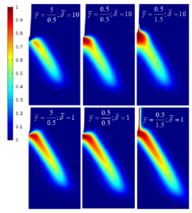
Interaction between fracture and martensitic PTs is a very important problem in the mechanics and physics of strength, transformational, and deformational materials properties. For example, the strong stress concentrator at the crack tip may cause nucleation of the product phase and initiate PTs [419, 48, 149, 75, 128, 329]. PT dissipates energy and produces transformation strain as a mechanism of inelastic deformation and elastic stress relaxation. This increases the resistance to the crack propagation and material ductility, which is coined the transformation toughening. Besides, stresses produced in the course of a PT may cause fracture, in particular during cyclic loading of SMAs [156]. PFA has been widely used for modeling fracture (see Section 19.5) and PTs (see Sections 11.4, 11.6 and 16), and their interaction [329, 48, 34, 35, 397, 473, 73]. However, only several papers [397, 473, 73, 177, 338] study both fracture and PT within the PFA. The most advanced PFA [177] is based on combination of PFAs to PT from [291], to fracture from [306], but most important, to surface-induced pre-transformations and transformations [309, 284], which leads to new nanoscale effects. In the PFA to surface-induced pre-transformations and transformations, numerous effects were found after transition from sharp external surface [308, 310] to a finite-width external surface described with a separate order parameter in [309, 284]. In PFA to fracture, free surfaces of finite width appear naturally, which makes it natural to integrate PFA to PT and fracture with PFA to surface-induced PT with a finite-width external surface in [309, 284]. Such a theory possesses two characteristic nanoscale parameters: widths of the crack surface and the interface width . Then the dimensionless scale parameter significantly affects PT and fracture, similar to other PFAs with two scale parameters, see Section 11.6 and [268, 269], Section 12 and [351, 277, 353, 354, 282], as well as review [251]. It was found that the lower surface energy of than that of (i.e., ) promotes nucleation of at the crack tip, its stabilization at the crack surface as a nanolayer (”wetting” by martensite), as well as nucleation of the pre-martensite or at the crack surfaces, even in the pseudoelastic regime, when stress release near the crack surface has to lead to the reverse PT (Fig. 28). In the opposite case, growth in the surface energy during PT inhibits the PT near the crack tip and at the crack surfaces, and displaces away from the crack tip in the pseudoelastic regime, and leads to reverse PT at the crack tip in the pseudoplastic regime.
From the other side, different surface energies of and influence the crack evolution through the change in cohesion and gradient energies, which affects crack nucleation location and propagation trajectory (branching) and the process of interfacial damage evolution (Fig. 29), as well as transformation toughening. All these variations are significantly affected by the dimensionless width and the surface energy . Consequently, these are two new parameters controlling coupled fracture and PTs.
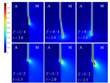
20 Concluding remarks
The presented review focuses on the various fundamental problems of PTs, CRs, and fracture in inelastic materials, which the author works last 30 years at. Within sharp interface approach, explicit expression for the thermodynamic driving force for SCs within a finite region in an inelastic material as well as extremum principle for finding all unknown parameters (position, shape, orientation of the transformed region, i.e., position of phase interfaces) are derived and discussed in Section 6. When a finite region represents volume covered by a moving interface during infinitesimal time increment, theory describes interface propagation in inelastic materials. This theory represents a nontrivial conceptual generalization of the theory for SCs in elastic materials. For elastic materials (see Section 4), the thermodynamic driving force for SCs is the gain in the Gibbs energy and all unknown parameters are determined by minimization of the Gibbs energy. While there were attempts to apply slightly modified Gibbs-energy-based theory to inelastic material, this is contradictory. It was demonstrated in Section 6 that the thermodynamic driving force for SCs in an inelastic material is the dissipation increment for the complete SC in the region under study due to SC only, i.e., the difference between the total dissipation increment and the dissipation increment due to all other dissipative processes but SC (e.g., plastic flow, evolution of internal variables, etc.). Instead of a surface-independent Eshelby integral in the theory of defects and path-independent J-integral in fracture mechanics, we introduced a region-independent integral for arbitrary inelastic materials. For an interface propagation, the driving force is not the Eshelby driving force but difference between the Eshelby driving force and dissipation due to other processes than SCs, in particularly, plasticity.
Special attention is devoted to kinetics of SCs, and three type of kinetics is considered: athermal or rate-independent kinetics, thermally-activated kinetics of appearance of the critical nucleus, and ”macroscale” thermally-activated kinetics, for which time for the appearance of a macroscale region is postulated. For each type of kinetics, the kinetic equation and extremum principle for determination of all unknown parameters are formulated. The athermal kinetics is the most close to the traditional approach to SCs in elastic materials: when all types of dissipation are neglected, the theory reduces to the Gibbs-energy-based theory for elastic materials. However, for inelastic materials, two solutions are always possible: with and without SCs. It was suggested to choose an actual solution with the help of the extremum principle for choosing the stable solution, which represents the global SC criterion. This additional principle does not have counterparts in elastic material, because for elastic materials solution corresponding to the minimum of the Gibbs energy is the actual one.
For other two cases, the Arrhenius-type kinetics for the time of SCs is utilized, and all unknown parameters are determined by the principle of the minimum of transformation time or its particular cases (e.g., the principle of minimum of activation energy or transformation mass (volume)). Since the Gibbs energy is not a driving force for inelastic materials, new definition of the activation energy was suggested. Again, kinetic approaches, when all types of dissipation are absent, reduce to kinetics of SCs in elastic materials. Since this kinetics was not broadly used in continuum approaches, it was presented in Section 4 as well. All extremum principles in this theory were derived using the postulate of realizability, presented in Section 6.5 for athermal kinetics and Section 6.8 for a macroscale thermally activated kinetics. In particular, the principle of the minimum of transformation time, which follows from the postulate of realizability, was intuitively used in material science and physical literature.
To illustrate the theory, various problems were solved analytically (even for large strains) or numerically in Sections 8 - 11, 14, and 15 for PTs and CRs, and in Section 19 for fracture and interaction between fracture and PT. Nontrivial points were related to various conditions at the phase interface (coherence, with sliding and/or decohesion), new approach to the incoherent phase interface, inheritance of plastic deformation during PTs and its effect on PT, introducing RIP, deriving analytical expression for TRIP and RIP at the propagating interface and in shear band, and martensite nucleation at the intersection of the shear bands. Virtual or intermediate melting, much (from 100 to 5000 K) below the thermodynamic melting temperature as a new mechanism of plastic deformation and stress relaxation during various PTs and high strain rate loading was recently revealed and is discussed in Sections 12 and 13.
Phase field approaches to PTs, twinning, dislocations and their interaction is presented in Section 16; PFA to fracture and interaction between fracture and PT is described in Section 19. PFAs described SCs in a continuous way by solving Ginzburg-Landau evolution equations for the order parameters. Special attention was devoted to strict continuum thermomechanical treatment of the PFA, which include formulation of new conditions for interpolation functions for all material properties, and satisfaction of these conditions. In contrast to sharp-interface approach, interfaces and defects have a finite width; there are no discontinuities and no needs to satisfy jump conditions across interfaces and develop special numerical procedures to track interface and defect motion. That is why very complex microstructure evolution (including splitting tips of martensitic variants, branching of cracks, and dendrite formation) can be reproduced by direct simulations without any a priory information. The PFA also includes additional information about stability and instability of phases and different states. All these items constitutes advantages of the PFA. Multiple solutions to various PFA problems are presented and new effects are revealed. At the same time, the sharp-interface approach gives specific expressions for the thermodynamic driving forces for nucleation and evolution of defects. It is convenient for solution of problems with relatively simple geometry of interfaces and defects, and allows analytical solutions for some problems.
PTs and CRs induced by large plastic shear under high pressure are reviewed in Section 17. It includes new material phenomena and four-scale approaches for their analyses, from atomistic studies to nano- and scale-free PFAs to microscale and macroscale modeling. This method of plastic treatment has strong potential for technological applications since plastic shear drastically (up to one to two order of magnitude) reduces PT and CR pressure and lead to new phases and reaction products that are not accessible under hydrostatic conditions.
Due to multifaceted physics and mechanics of the interaction between PTs, CRs, and fracture with plasticity, many aspects were not covered properly or covered at all. In particular, such an interaction at the crystal plasticity and macroscopic levels, while shortly discussed in Section 18, requires much more attention. Sharp-interface approach to fracture in elastoplastic materials is covered as an illustration of our general thermodynamic and kinetic approaches only, while many other approaches are developed in literature. Experimental, especially modern in situ methods, at different scales, should be discussed separately. There is also huge literature on lithium-ion batteries, in particular, silicon based, which includes large elastoplasticity of Si during lithiation/delithiation and corresponding chemical reactions.
Most of the problems discussed in the review are far from being fully resolved; many of them are in their infancy.
Complexity and multidisciplinary and multifaceted character of the problems on interaction between various SCs and plasticity as well as their applied significance will definitely attract a lot of attention from researches from various disciplines working at multiple scales.
Acknowledgements
The author worked for more than three decades on various aspects of the topic of the current review. This work was initiated in 1988 at the Institute for Superhard Materials of the Ukrainian Academy of Sciences, Kiev, Ukraine with support from the Ukrainian Academy of Sciences. Special thanks is to Prof. Nikolay V. Novikov, director of the Institute, supervisor of the author’s PhD work (1978-1981), who played very important role in formation of the author’s interests, and with whom authors continued working till 1993 and closely communicating after. This work was continued during 1992-1999 at the University of Hannover (Germany) with support from the Alexander von Humboldt Foundation, Volkswagen Foundation, and German Research Society. In the USA, at Texas Tech University (1999-2008) and currently at Iowa State University, this work was supported by National Science Foundation, Army Research Office, Office of Naval Research, Defense Advanced Research Projects Agency, Defense Threat Reduction Agency, Los Alamos National Laboratory, National Institute of Standards and Technology, Geophysical Laboratory of Carnegie Institution of Washington, and Air Force Office of Scientific Research, as well as Schafer 2050 Challenge Professorship (2008-2017) and Vance Coffman Faculty Chair Professor in Aerospace Engineering (2017- ). Current support used for writing this review was obtained from NSF (CMMI-1943710 and DMR-1904830), ONR (N00014-19-1-2082), ARO (W911NF-17-1-0225), and Iowa State University (Vance Coffman Faculty Chair Professorship). The author greatly appreciates and enjoyed collaboration with all his coauthors of papers cited here, including graduate students, post docs, and faculty and researchers from different organizations.
References
- Abeyaratne and Knowles, [1990] Abeyaratne, R., Knowles, J.K., 1990, On the driving traction acting on a surface of strain discontinuity in a continuum, J. Mech. Phys. Solids 38, 345-360.
- Ambati et al., [2015] Ambati, M., Gerasimov, T., De Lorenzis, L., 2015. Phase-field modeling of ductile fracture. Computational Mechanics 55, 1017-1040.
- Ambati et al., [2016] Ambati, M., Kruse, R., De Lorenzis, L., 2016. A phase-field model for ductile fracture at finite strains and its experimental verification. Computational Mechanics 57, 149-167.
- Amor et al., [2009] Amor, H., Marigo, J.-J., Maurini, C., 2009. Regularized formulation of the variational brittle fracture with unilateral contact: numerical experiments. Journal of the Mechanics and Physics of Solids 57, 1209-1229.
- An et al., [2008] An, Q., Luo, S.N., Han, L.-B., Zheng, L., Tschaunerc, O., 2008. Melting of Cu Under Hydrostatic and Shock Wave Loading to High Pressures. J. Phys.: Cond. Mat. 20, 095220.
- Appolaire et al., [2010] Appolaire, B., Aeby-Gautier, E., Da Costa Teixeira, J., Dehmas, M., Denis, S., 2010. Non-coherent interfaces in diffuse interface models, Philosophical Magazine, 90, 461-483.
- Aranson et al., [2000] Aranson, I.S., Kalatsky, V.A., Vinokur, V.M., 2000. Continuum Field Description of Crack Propagation. Physical Review Letters 85, 118-121.
- Arbib et al., [2020] Arbib, E., Biscari, P., Bortoloni, L., Patriarca, C., Zanzotto, G. 2020. Crystal elasto-plasticity on the Poincare half-plane. International Journal of Plasticity, 130, 102728.
- Armetev et al, [2001] Artemev, A., Jin, Y., Khachaturyan, A.G., 2001. Three-dimensional phase field model of proper martensitic transformation. Acta. Mater. 49, 1165-1177.
- Asaro, [1983] Asaro, R.J., 1983. Crystal plasticity. J. Appl. Mech., 50, 921-934.
- Atluri, [1997] Atluri, S.N., 1997. Structural Integrity and Durability (Forsyth: Tech Science Press).
- Babaei and Levitas, [2018] Babaei, H., Levitas, V.I., 2018. Phase field approach for stress- and temperature-induced phase transformations that satisfies lattice instability conditions. Part 2. Simulations of phase transformations Si ISi II. International Journal of Plasticity, 107, 223-245.
- Babaei and Levitas, [2019] Babaei, H., Levitas, V.I., 2019. Effect of 60o dislocation on transformation stresses, nucleation, and growth for phase transformations between silicon I and silicon II under triaxial loading: phase-field study. Acta Materialia, 177, 178-186.
- Babaei et al., [2019] Babaei H., Basak A., and Levitas V.I., 2019. Algorithmic aspects and finite element solutions for advanced phase field approach to martensitic phase transformation under large strains. Computational Mechanics, 64, 1177-1197.
- Baggio et al., [2019] Baggio, R., Arbib, E., Biscari, P., Conti, S., Truskinovsky, L., Zanzotto, G., Salman, O. U. 2019. Landau-Type Theory of Planar Crystal Plasticity. Physical Review Letters, 123, 205501.
- Ball and James, [1992] Ball, J., James, R.D., 1992. Proposed experimental tests of a theory of fine microstructure and the two-well problem. Philos. Trans. 338, 389-450.
- Bar’yachtar et al., [1986] Bar’yachtar, V.G., Enilevskiy, S.G., Tokiy, V.V., Jablonsky, D.A., 1986. Thermodynamical theory of nucleation in the elastoplastic media. Sov. Phys. Solid State 28, 1303-1310.
- Barsch and Krumhansl, [1984] Barsch, G.R., Krumhansl, J.A., 1984. Twin boundaries in ferroelastic media without interface dislocations. Phys. Rev. Lett. 53, 1069-1072.
- Bartel et al., [2011] Bartel, T., Menzel, A., Svendsen, B., 2011. Thermodynamic and relaxation-based modeling of the interaction between martensitic phase transformations and plasticity. J. Mech. Phys. Solids. 59, 1004-1019.
- Barton et al., [2005] Barton, N.R., Benson, D.J., Becker, R., 2005. Crystal level continuum modelling of phase transformations: the transformation in iron. Model. Simulat. Mater. Sci. Eng. 13, 707–731.
- Basak and Levitas, [2018] Basak A. and Levitas V. I. 2018. Nanoscale multiphase phase field approach for stress and temperature-induced martensitic phase transformations with interfacial stresses at finite strains. Journal of the Mechanics and Physics of Solids, 2018, 113, 162-196.
- Basak and Levitas, [2017] Basak A. and Levitas V.I., 2017. Interfacial stresses within boundary between martensitic variants: Analytical and numerical finite strain solutions for three phase field models. Acta Materialia, 139, 174-187.
- Basak and Levitas, [2019] Basak A. and Levitas V.I., 2019. Finite element procedure and simulations for a multiphase phase field approach to martensitic phase transformations at large strains and with interfacial stresses. Computer Methods in Applied Mechanics and Engineering, 343, 368-406.
- Beese and Mohr, [2011] Beese, A.M., Mohr, D., 2011. Effect of stress triaxiality and Lode angle on the kinetics of strain-induced austenite-to-martensite transformation. Acta Materialia 59, 2589-2600.
- Battacharyya and Weng, [1994] Bhattacharyya, A., Weng, G.J., 1994. An Energy Criterion for the Stress-Induced Martensitic Transformation in a Ductile System. J. Mech. Phys. Solids 42, 1699-1724.
- Battacharyya, [2003] Bhattacharya, K., 2003. Microstructure of Martensite. Why it Forms and How It Gives Rise to the Shape-Memory Effect. Oxford University Press.
- Biscari et al., [2015] Biscari, P., Urbano, M. F., Zanzottera, A., Zanzotto, G., 2015. Intermittency in crystal plasticity informed by lattice symmetry. J. Elasticity, 123, 85-96.
- Blank and Estrin, [2014] Blank, V.D., Estrin, E.I., 2014, Phase Transitions in Solids under High Pressure, CRC Press, Boca Raton.
- Blank et al., [1994] Blank, V.D., Popov, M., Buga, S.G., Davydov, V., Denisov, V.N., Ivlev, A.N., Mavrin, B.N., Agafonov, V., Ceolin, R., Szwarc, H., Passat, A., 1994. Is Fullerite Harder than Diamond? Physics Letters A 188, 281-286.
- Boguslavskiy, [1985] Boguslavskiy, Y.Y., 1985. Formation of coherent and partially coherent nucleus at phase transition under conditions of nonhydrostatic compression. Solid State Physics 27, 140-143.
- Bollada et al., [2012] Bollada, P.C., Jimack, P.K., Mullis, A.M., 2012. A new approach to multi-phase formulation for the solidification of alloys. Physica D 241, 816-829.
- Borden et al., [2014] Borden, M.J., Hughes, T.J.R., Landis, C.M., Verhoosel, C.V., 2014. A higher-order phase-field model for brittle fracture: Formulation and analysis within the isogeometric analysis framework. Computer Methods in Applied Mechanics and Engineering 273, 100-118.
- Boulbitch and Toledano, [1998] Boulbitch, A.A., Toledano, P., 1998. Phase Nucleation of Elastic Defects in Crystals Undergoing a Phase Transition, Physical Review Letters 81, 838.
- Boulbitch and Korzhenevskii, [2016] Boulbitch, A., Korzhenevskii, A.L., 2016. Field-theoretical description of the formation of a crack tip process zone. The European Physical Journal B 89, 261.
- Boulbitch et al., [2017] Boulbitch, A., Gufan, Y.M., Korzhenevskii, A.L., 2017. Crack-tip process zone as a bifurcation problem. Physical Review E 96, 013005.
- Bourdin et al., [2000] Bourdin, B., Francfort, G.A., Marigo, J.J., 2000. Numerical experiments in revisited brittle fracture. Journal of the Mechanics and Physics of Solids 48, 797-826.
- Bourdin et al., [2011] Bourdin, B., Larsen, C.J., Richardson, C.L., 2011. A time-discrete model for dynamic fracture based on crack regularization. International journal of fracture 168, 133-143.
- Bowlan et al., [2019] Bowlan, P., Henson, B.F., Smilowitz, L., Levitas, V.I., Suvorova, N., Oschwald, D., 2019. Kinetics of the - phase transition in energetic nitramine-octahydro-1,3,5,7-tetranitro-1,3,5,7-tetrazocine. Journal of Chemical Physics 159, 064705.
- Boyko et al., [1997] Boyko, V., Garber, R., Kossevich, A., 1997. Reversible Crystal Plasticity, AIP, New York.
- Brainin et al., [1981] Brainin, G. E. and Likhachev, V.A., 1982. Crystallography of Dislocations Inherited in Martensitic Transformations and Twinning. Physics of Metals, 4, No. 3, 489-502.
- [41] Bridgman, P.W., 1937. Shear Phenomena at High Pressure, Particular Inorganic Compounds. Proc. Am. Acad. Arts Sci. 71, 387
- [42] Bridgman, P.W., 1947. The Effect of High Mechanical Stress on Certain Solid Explosives. J. Chem. Phys. 15, 311-313
- Britun and Kurdyumov, [2000] Britun, V.F., Kurdyumov, A.V., 2000. Mechanisms of martensitic transformations in boron nitride and conditions of their development. High Pressure Research 17, 101-111.
- Britun and Kurdyumov, [2002] Britun, V.F., Kurdyumov, A.V., 2002. Analysis of the effect of nonhydrostatic compression conditions on direct phase transformations in carbon. Powder Metallurgy and Metal Ceramics 41, 417-423.
- Budnitzki and Kuna, [2016] Budnitzki, M., Kuna, M. 2016. Stress induced phase transitions in silicon. Journal of the Mechanics and Physics of Solids, 95, 64-91.
- Budzevich et al., [2012] Budzevich, M.M., Zhakhovsky, V.V., White, C.T., Oleynik, I.I., 2012. Evolution of Shock-Induced Orientation-Dependent Metastable States in Crystalline Aluminum. Phys. Rev. Lett. 109, 125505.
- Bulatov and Cai, [2006] Bulatov, V.V., Cai, W., 2006. Computer Simulation of Dislocations. Oxford Series on Materials Modelling (Oxford: Oxford University Press).
- Bulbich, [1992] Bulbich, A.A., 1992. Nucleation on the crack tip and transformation toughness in crystals undergoing structural phase transitions. Journal of Materials Science 27, 1070-1080.
- Bundy, [1989] Bundy, F.P., 1989. Behavior of elemental carbon up to very high temperatures and pressures. High Pressure Science and Technology, Proceedings of the XI AIRAPT International Conference 1, ed N V Novikov, 326-336 (Kiev: Naukova Dumka).
- Cermelli and Gurtin, [1994] Cermelli, P., Gurtin, M.E., 1994. On the kinematics of incoherent phase transitions. Acta Metallurgica et Materialia 42, 3349-3359.
- Chen et al., [2020] Chen, H., Zarkevich, N. A., Levitas, V. I., Johnson, D. D., X. Zhang. 2020. Fifth-degree elastic potential for predictive stress-strain relations and elastic instabilities under large strain and complex loading in Si. NPJ Computational Materials, 6, 115.
- Chen et al., [2019] Chen H., Levitas V.I., Xiong L., 2019. Amorphization Induced by 60o Shuffle Dislocation Pileup against Tilt Grain Boundaries in Silicon Bicrystal under Shear. Acta Mater. 179, 287-295.
- Chen et al., [2019] Chen, H., Levitas, V.I., Xiong, L., 2019. Slip of Shuffle Screw Dislocations through Tilt Grain Boundaries in Silicon. Computational Materials Science 1, 132-135.
- Chen, [2002] Chen, L.Q., 2002. Phase-field models for microstructure evolution. Annu. Rev. Mater. Res. 32, 113-140.
- Cherepanov, [1967] Cherepanov, G.P., 1967. On crack propagation in continuous media. J. Appl. Math. and Mech. (PMM) 31, 476-488.
- Cherepanov, [1979] Cherepanov, G.P., 1979. Mechanics of Brittle Fracture (New York: McGraw-Hill).
- Cherepanov, [1997] Cherepanov, G.P., 1997. Methods of Fracture Mechanics: Solid Matter Physics (Dordrecht: Kluwer Academic Publishers).
- [58] Cherkaoui, M., Berveiller, M., 2000a. Micromechanical modeling of the martensitic transformation induced plasticity in steels. Smart Materials and Structures 9, 592-603.
- [59] Cherkaoui, M., Berveiller, M., 2000b. Moving inelastic discontinuities and applications to martensitic phase transition. Archive of Applied Mechanics 70, 159-181.
- Cherkaoui et al., [1998] Cherkaoui, M., Berveiller, M., Sabar, H., 1998. Micromechanical modeling of the martensitic transformation induced plasticity (TRIP) in austenitic single crystals. International Journal of Plasticity 14, 597-626.
- Chistotina et al., [1970] Chistotina, N.P., Zharov, A.A., Kissin Y.V., Enikolopyan, N.S., 1970. Polymerization of benzol under conditions of superhigh pressure in combination with shear strain. Doklady Akademii Nauk SSSR 191, 632-634.
- Chluba et al., [2015] Chluba, C., Ge, W., Lima de Miranda, R., Strobel, J., Kienle, L., Quandt, E., Wuttig, M., 2015. Ultralow-fatigue shape memory alloy films. Science 348, 1004-1007.
- Cho et al., [2012] Cho, J.Y., Idesman, A.V., Levitas, V.I., Park, T., 2012. Finite element simulations of dynamics of multivariant martensitic phase transitions based on Ginzburg-Landau theory. Int. J. Solids Struct. 49, 1973-1992.
- Cho et al., [2012] Cho, J. Y., Idesman, A. V., Levitas, V. I., Park, T. 2012. Finite element simulations of dynamics of multivariant martensitic phase transitions based on Ginzburg-Landau theory. Int. J. Solids Struct. 49, 1973-1992.
- Chowdhury and Sehitoglu, [2017] Chowdhury, P., Sehitoglu, H., 2017. A revisit to atomistic rationale for slip in shape memory alloys. Progress in Materials Science 85, 1-42.
- Christian, [1965] Christian, J.W., 1965. The Theory of Transformation in Metals and Alloys (Oxford: Pergamon Press).
- Ciss and Zaeem, [2020] Ciss, C., Zaeem, M. A., 2020. A phase-field model for non-isothermal phase transformation and plasticity in polycrystalline yttria-stabilized tetragonal zirconia. Acta Materialia, 191, 111-123.
- Cisseand Zaeem, [2020] Cissé, C., Zaeem, M.A., 2020. On the elastocaloric effect in CuAlBe shape memory alloys: A quantitative phase-field modeling approach. Computational Materials Science 183, 109808.
- [69] Clayton, J. D., Knap, J., 2011a. A phase field model of deformation twinning: nonlinear theory and numerical simulations. Phys. D. 240, 841-858.
- [70] Clayton, J.D., Knap, J., 2011b. Phase field modeling of twinning in indentation of transparent crystals. Model. Simul. Mater. Sci. Eng. 19, 085005.
- Clayton and Knap, [2013] Clayton, J. D., Knap, J., 2013. Phase-field analysis of fracture-induced twinning in single crystals. Acta Materialia 61, 5341-5353.
- Clayton and Knap, [2016] Clayton, J.D., Knap, J., 2016. Phase field modeling and simulation of coupled fracture and twinning in single crystals and polycrystals. Computer Methods in Applied Mechanics and Engineering 312, 447-467.
- Clayton, [2019] Clayton, J., 2019. Computational Modeling of Dual-Phase Ceramics with Finsler-Geometric Phase Field Mechanics. Computer Modeling in Engineering and Sciences 120, 333-350.
- Cottura et al., [2012] Cottura, M., Le Bouar, Y., Finel, A., Appolaire, B., Ammar, K., Forest, S., 2012. A phase field model incorporating strain gradient viscoplasticity: Application to rafting in Ni-base superalloys. J. Mech. Phys. Solids 60, 1243-1256.
- Creuziger et al., [2008] Creuziger, A., Bartol, L.J., Gall, K., Crone, W.C., 2008. Fracture in single crystal NiTi. Journal of the Mechanics and Physics of Solids 56, 2896-2905.
- Cui et al., [2018] Cui, S., Wan, J., Zhang, J., Chen, N., Rong, Y. 2018. Phase-field study of microstructure and plasticity in polycrystalline MnNi shape memory alloys, Metall. Mater. Trans. A. 49, 5936-5941.
- Cui et al., [2006] Cui, J., Chu, Y.S., Famodu, O.O., Furuya, Y., Hattrick-Simpers, J., James, R.D., Ludwig, A., Thienhaus, S., Wuttig, M., Zhang, Z., Takeuchi, I., 2006. Combinatorial search of thermoelastic shape memory alloys with extremely small hysteresis width. Nat. Mater. 5, 286-290.
- Das et al., [2016] Das, Y.B., Forsey, A.N., Simm, T.H., Perkins, K.M., Fitzpatrick, M.E., Gungor, S., Moat, R.J., 2016. In situ observation of strain and phase transformation in plastically deformed 301 austenitic stainless steel. Materials and Design 112, 107-116.
- Datta et al., [1986] Datta, R., Ghosh, G., Raghavan, V., 1986. Plastic accommodation during growth of the martensitic plates in Fe-Ni alloys. Scripta Metallurgica 20, 559-563.
- Denoual et al., [2010] Denoual, C., Caucci, A.M., Soulard, L., Pellegrini, Y. P., 2010. Phase-field reaction-pathway kinetics of martensitic transformations in a model Fe3Ni alloy. Phys. Rev. Lett. 105, 035703.
- Denoual and Vattré, [2016] Denoual, C., Vattré, A., 2016. A phase field approach with a reaction pathways-based potential to model reconstructive martensitic transformations with a large number of variants. J. Mech. Phys. Solids, 90, 91-107 .
- Diani and Parks, [1998] Diani, J.M., Parks, D.M., 1998. Effects of strain state on the kinetics of strain-induced martensite in steels. Journal of Mechanics and Physics of Solids 46, 1613-1635.
- Dittmann et al., [2018] Dittmann, M., Aldakheel, F., Schulte, J., Wriggers, P., Hesch, C., 2018. Variational phase-field formulation of non-linear ductile fracture. Computer Methods in Applied Mechanics and Engineering 342, 71-94.
- Dremov et al., [2015] Dremov, V.V., Rykounov, A.A., Sapozhnikov, F.A., Karavaev, A.V., Yakovlev, S.V., Ionov, G.V., Ryzhkov, M.V., 2015. Cold melting of beryllium: Atomistic view on Z-machine experiments. Journal of Applied Physics 118, 035901.
- Duda et al., [2015] Duda, F.P., Ciarbonetti, A., Sánchez, P.J., Huespe, A., 2015. A phase-field/gradient damage model for brittle fracture in elastic-plastic solids. International Journal of Plasticity 65, 269-296.
- Dugdale, [1960] Dugdale, D.S., 1960. Yielding of steel sheets containing slits. J. Mech. Phys. Solids8, 100-104.
- Edalati, [2016] Edalati K. and Horita Z. 2016. A review on high-pressure torsion (HPT) from 1935 to 1988, Mat. Sci. Eng. A., 652, 325-352.
- Enikolopyan, [1985] Enikolopyan, N.S., 1985. Some aspects of chemistry and physics of plastic flow. Pure and Applied Chemistry 57, 1707-1711.
- Enikolopyan, [1989] Enikolopyan, N.S., 1989. Super-fast chemical reactions in solids. Russian Journal of Physical Chemistry 63, 1261-1265.
- Esfahani et al., [2018] Esfahani S.E., Ghamarian I., Levitas V.I., Collins P.C., 2018. Microscale Phase Field Modeling of the Martensitic Transformation During Cyclic Loading of NiTi Single Crystal. International Journal of Solids and Structures 146, 80-96.
- Esfahani et al., [2018] Esfahani S.E., Ghamarian I., Levitas V.I., Collins P.C. 2018. Microscale Phase Field Modeling of the Martensitic Transformation During Cyclic Loading of NiTi Single Crystal. International Journal of Solids and Structures, 146, 80-96.
- Esfahani et al., [2020] Esfahani S.E., Ghamarian I., Levitas V.I., 2020. Strain-induced multivariant martensitic transformations: A scale-independent simulation of interaction between localized shear bands and microstructure. Acta Mater. 196, 430-433.
- Eshelby, [1970] Eshelby, J.D., 1970. Energy relations and the energy-momentum tensor in continuum mechanics. Inelastic Behaviour of Solids, eds M F Kanninen et al, 77-115 (New York: McGraw-Hill).
- Eshelby, [1951] Eshelby, J.D., 1951. The force on an elastic singularity. Phil. Trans. Roy. Soc. A 244, 87-111.
- Eshelby, [1956] Eshelby, J.D., 1956. The continuum theory of lattice defects. Solid State Physics 3, 79-144 (New York: Academic Press).
- Eshelby, [1957] Eshelby, J.D., 1957. The determination of the elastic field of an ellipsoidal inclusion, and related problems. Proceedings of the Royal Society A 241, 376-396.
- Eshelby, [1970] Eshelby, J.D., 1970. Energy relations and the energy-momentum tensor in continuum mechanics. Inelastic Behaviour of Solids, eds M F Kanninen, W F Adler, A R Rosenfield and R I Jaffee, 77-115. (New York: McGraw-Hill).
- Falk, [1983] Falk, F. 1983. One-dimensional model of shape memory alloy. Arch. Mech. 15, 63-84.
- Falk and Konopka, [1990] Falk, F., Konopka, P., 1990. Three-dimensional Landau theory describing the martensitic phase transformation of shape memory alloys. J. Phys.: Condens. Matter 2, 61-77.
- Feng and Levitas, [2017] Feng, B., Levitas, V. I., 2017. Coupled Elastoplasticity and Strain-Induced Phase Transformation under High Pressure and Large Strains: Formulation and Application to BN Sample Compressed in a Diamond Anvil Cell. Int. J. Plast, 96, 156-181.
- Feng and Levitas, [2017] Feng, B., Levitas, V. I., 2017. Large elastoplastic deformation of a sample under compression and torsion in a rotational diamond anvil cell under megabar pressures. International Journal of Plasticity, 92, 79-95.
- Feng et al., [2019] Feng, B., Levitas, V. I., Li, W. 2019. FEM modeling of plastic flow and strain-induced phase transformation in BN under high pressure and large shear in a rotational diamond anvil cell. International Journal of Plasticity, 113, 236-254.
- Feng et al., [2016] Feng, B., Levitas, V. I., Hemley, R. J. 2016. Large elastoplasticity under static megabar pressures: Formulation and application to compression of samples in diamond anvil cells. Int. J. Plast. 84, 33-57.
- Feng and Levitas, [2018] Feng, B., Levitas, V. I. 2018. Finite-element simulations of elastoplastic flow during compression of a sample in a diamond anvil cell under extremely high pressure: Effects of geometry and material properties. Physical Review Applied, 10, 064060.
- Feng et al., [2018] Feng, B., Bronkhorst, C.A., Addessio, F.L., Morrow, B.M., Cerreta, E.K., Lookman, T., Lebensohn, R.A., Low, T., 2018. Coupled elasticity, plastic slip, and twinning in single crystal titanium loaded by split-Hopkinson pressure bar. Journal of the Mechanics and Physics of Solids 119, 274-297.
- [106] Feng, B., Bronkhorst, C.A., Liu, Z., Morrow, B.M., Cerreta, E.K., Li, W.H., Daphalapurkar, N.P., 2020a. Three-dimensional modeling and simulations of single-crystal and bi-crystal titanium for high-strain-rate loading conditions. International Journal of Plasticity 133, 102771.
- [107] Feng, Z., Zecevic, M., Knezevic, M., 2020. Stress-assisted () and strain-induced () phase transformation kinetics laws implemented in a crystal plasticity model for predicting strain path sensitive deformation of austenitic steels. International Journal of Plasticity, 136, 102807.
- Fisher, [1948] Fischer, J.C., 1948. The fracture of liquids. Journal of Applied Physics 19, 1062-1067.
- Fischer and Antretter, [2009] Fischer, F.D., Antretter, T., 2009. Deformation, stress state and thermodynamic force for a growing void in an elastic-plastic material. International Journal of Plasticity 25, 1819-1832.
- Fischer et al., [1994] Fischer, F.D., Berveiller, M., Tanaka, K., Oberaigner, E., 1994. Continuum mechanical aspects of phase transformations in solids. Archive of Applied Mechanics 64, 54-85.
- Fischer and Oberaigner, [2000] Fischer, F.D., Oberaigner, E.R., 2000. Deformation, stress state, and thermodynamic force for a transforming spherical inclusion in an elastic-plastic material. Journal of Applied Mechanics 67, 793-796.
- Fischer and Oberaigner, [2001] Fischer, F.D., Oberaigner, E.R., 2001. A micromechanical model of phase boundary movement during solid-solid phase transformations. Archive of Applied Mechanics 71, 193-205.
- Fischer et al., [1996] Fischer, F.D., Sun, Q.-P., Tanaka, K., 1996. Transformation-Induced Plasticity (TRIP). Applied Mechanics Reviews 49, 317-364.
- Fischer and Reisner, [1998] Fischer, F.D., and Reisner, G., 1998. A Criterion for the Martensitic Transformation of a Microregion in an Elastic-Plastic Material. Acta Materialia 46, 2095-2102.
- Fischer et al., [2000] Fischer, F.D., Reisner, G., Werner, E., Tanaka, K., Cailletaud, G., Antretter, T., 2000. A new view on transformation induced plasticity (TRIP). International Journal of Plasticity 16, 723-748.
- Fischer et al., [2008] Fischer, F.D., Waitz, T., Vollath, D., Simha, N.K., 2008. On the role of surface energy and surface stress in phase-transforming nanoparticles. Progress in Materials Science 53, 481-527.
- Folch and Plapp, [2003] Folch, R., Plapp, M., 2003. Towards a quantitative phase-field model of two-phase solidification. Phys. Rev. E. 68, 010602.
- Folch and Plapp, [2005] Folch, R., Plapp, M., 2005. Quantitative phase-field modeling of two-phase growth. Phys. Rev. E. 72, 011602.
- Francfort and Marigo, [1998] Francfort, G.A., Marigo, J.J., 1998. Revisiting brittle fracture as an energy minimization problem. Journal of the Mechanics and Physics of Solids 46, 1319-1342.
- Frost and Ashby, [1989] Frost, H.J., Ashby, M.F., 1989. Deformation-mechanism maps (New York: Pergamon Press).
- Ganghoffer et al., [1991] Ganghoffer, J.F., Denis, S., Gautier, E., Simon, A., Simonsson, K., Sjöström, S., 1991. Micromechanical simulation of a martensitic transformation by finite element. Journal de Physique IV, Colloque C4, supplment au Journal de Physique III 1, 83-88.
- Gao et al., [2019] Gao, Y., Ma, Y., An, Q., Levitas, V.I., Zhang, Y., Feng, B., Chaudhuri, J., Goddard, III W.A., 2019. Shear driven formation of nano-diamonds at sub-gigapascals and 300 K. Carbon 146, 364-368.
- Garcke et al., [1999] Garcke, H., Nestler, B., Stoth, B., 1999. A multiphase field concept: Numerical simulations of moving phase boundaries and multiple junctions. Phys. Rev. B. 78, 024113.
- Geslin, et al., [2014] Geslin, P.A., Appolaire, B., Finel, A., 2014. Investigation of coherency loss by prismatic punching with a nonlinear elastic model. Acta Materialia 71, 80-88.
- [125] Ghosh, G., Olson, G.B., 1994a. Kinetics of F.C.C. B.C.C. heterogeneous martensitic nucleation. Part I. The critical driving force for athermal nucleation. Acta Metallurgica et Mateialia 42, 3361-3370.
- [126] Ghosh, G., Olson, G.B., 1994b. Kinetics of F.C.C. B.C.C. heterogeneous martensitic nucleation. Part II. Thermal activation. Acta Metallurgica et Materialia 42, 3371-3379.
- Ghosh and Raghavan, [1986] Ghosh, G., Raghavan, V., 1986. The dimensions of isothermally formed martensitic plates in an Fe-Ni-Mn alloy. Materials Science and Engineering 79, 223-231.
- Gollerthan et al., [2009] Gollerthan, S., Young, M.L., Neuking, K., Ramamurty, U., Eggeler, G., 2009. Direct physical evidence for the back-transformation of stress-induced martensite in the vicinity of cracks in pseudoelastic NiTi shape memory alloys. Acta Materialia 57, 5892-5897.
- Grinfeld, [1980] Grinfeld, M.A., 1980. Conditions for thermodynamic phase equilibrium in a nonlinear elastic material. Doklady Akad. Nauk SSSR 88, 10-14.
- Grinfeld, [1991] Grinfeld, M.A., 1991. Thermodynamic Methods in the Theory of Heterogeneous Systems (Sussex: Longman).
- Gröger et al., [2008] Gröger, R., Lookman, T., Saxena, A., 2008. Defect-induced incompatibility of elastic strains:Dislocations within the Landau theory of martensitic phase transformations. Phys. Rev. B. 78, 184101.
- Gröger et al., [2016] Gröger, R., Marchand, B., Lookman, T., 2016. Dislocations via incompatibilities in phase-field models of microstructure evolution. Phys. Rev. B. 94, 054105.
- Grujicic and Olson, [1998] Grujicic, M., Olson, G.B., 1998. Dynamics of martensitic interfaces. Interface Science 6, 155-164.
- Grujicic et al., [1985] Grujicic, M., Olson, G.B., Owen, W.S., 1985. Mobility of martensitic interfaces. Metallurgical Transaction A 16A, 1713-1722.
- Gunkelmann et al., [2012] Gunkelmann, N., Bringa, E.M., Kang, K., Ackland, G.J., Ruestes, C.J., Urbassek, H.M., 2012. Polycrystalline iron under compression: plasticity and phase transitions. Phys. Rev. B 86, 144111.
- Gunkelmann et al., [2014] Gunkelmann, N., Bringa, E.M., Tramontina, D.R., Ruestes, C.J., Suggit, M.J., Higginbotham, A., Wark, J.S., Urbassek, H.M., 2014. Shock waves in polycrystallineiron: plasticity and phase transitions. Phys. Rev. B 89, 140102.
- Gunkelmann et al., [2014] Gunkelmann, N., Bringa, E. M., Tramontina, D. R., Ruestes, C. J., Suggit, M. J., Higginbotham, A., Wark, J. S., Urbassek, H. M. 2014. Shock waves in polycrystalline iron: plasticity and phase transitions. Phys. Rev. B. 89, 140102.
- Gunkelmann et al., [2012] Gunkelmann, N., Bringa, M. B., Kang, K., Ackland, G. J. 2012. Polycrystalline iron under compression: plasticity and phase transitions. Phys. Rev. B. 86, 144111.
- Gunkelmann et al., [2014] Gunkelmann, N., Tramontina, D. R., Bringa, E. M., Urbassek, H. M. 2014. Interplay of plasticity and phase transformation in shock wave propagation in nanocrystalline iron. New J. Phys. 16, 093032.
- Guo et al., [2005] Guo, X.H., Shi, S.Q., Ma, X.Q., 2005. Elastoplastic phase field model for microstructure evolution. Applied Physics Letters 87, 221910.
- Gurtin, [2000] Gurtin, M.E., 2000. Configurational Force as a Basic Concept of Continuum Physics (New York: Springer-Verlag).
- Gurtin and Murdoch, [1975] Gurtin, M.E., Murdoch, A., 1975. A continuum theory of elastic material surfaces. Arch. Rational Mech. Anal. 57, 291-323.
- Gurtin and Struthers, [1990] Gurtin, M.E., Struthers, A., 1990. Multiphase thermomechanics with interfacial structure 3. Evolving phase boundaries in the presence of bulk deformation. Arch. Rational Mech. Anal. 112, 97-160.
- Haezebrouck, [1987] Haezebrouck, D.M., 1987. Doctoral Thesis. Nucleation and Growth of a Single Martensitic Particle. (Evanston: Northwestern University, Materials Research Center, Steel Research Group)
- Hahn et al., [2016] Hahn, E., Zhao, S., Bringa, E., Meyers, M. 2016. Supersonic dislocation bursts in silicon. Sci. Rep. 6, 26977.
- Hakim and Karma, [2005] Hakim, V., Karma, A., 2005. Crack Path Prediction in Anisotropic Brittle Materials. Physical Review Letters 95, 235501.
- Hakim and Karma, [2009] Hakim, V., Karma, A., 2009. Laws of crack motion and phase-field models of fracture. Journal of the Mechanics and Physics of Solids 57, 342-368.
- Hammerberg et al., [2003] Hammerberg, J.E., Ravelo, R., Germann, T.C., Kress, J.D., Holian, B.L., 2003. Sliding Friction at Compressed Ta/Al Interfaces. Shock Compression of Condenced Matter: AIP Conf. Proc. 706, eds M D Furnish, Y. M. Gupta and J. W. Forbes, 565-568.
- Hangen and Sauthoff, [1999] Hangen, U.D., Sauthoff, G., 1999. The effect of martensite formation on the mechanical behaviour of NiAl. Intermetallics 7, 501-510.
- Harrison, [1980] Harrison, J.D., 1980. The ”State-of-the-Art” in crack tip opening displacement testing and analysis. The Welding Institute Members Report 108.
- He et al., [2014] He, A.M., Wang, P., Shao, J.L., Duan, S.Q., Zhao, F.P., Luo, S.N., 2014. Solid-liquid phase transitions in single crystal Cu under shock and release conditions. J. Appl. Phys. 115, 143503.
- Hecker et al., [1982] Hecker, S.S., Stout, M.G., Staudhammer, K.P., Smith, J.L., 1982. Effects of Strain State and Strain Rate on Deformation-Induced Transformation in 304 Stainless Steel: Part I. Magnetic Measurements and Mechanical Behavior. Metallurgical Transactions A 13, 619-626.
- Henry and Levine, [2004] Henry, H., Levine, H., 2004. Dynamic instabilities of fracture under biaxial strain using a phase field model. Physical review letters 93, 105504.
- Hill, [1950] Hill, R., 1950. Mathematical Theory of Plasticity (Oxford: Clarendon Press).
- Hirth and Lothe, [1992] Hirth, J.P., and Lothe, J., 1992. Theory of Dislocations (Malabar, Florida: Krieger Publishing Company).
- Hornbogen, [1991] Hornbogen, E., 1991. Legierungen mit Formgedächtnis. Rheinisch-Westfälische Akademie der Wissenschaften Vorträge 338 (Opladen: Westdeutcher Verlag).
- Hornbogen, [1997] Hornbogen, E., 1997. Ausforming and Marforming of SMA. Int. Conference on Displacive Phase Transitions and their Application in Material Engineering, eds K Mukherjee et al, 27-35 (TMS).
- Hou et al., [2019] Hou H., Simsek E., Ma T., Johnson N. S., Qian S., Cissé C., Stasak D., Hasan N. A., Zhou L., Hwang Y., Radermacher R., Levitas V. I., Kramer M. J., Zaeem M. A., Stebner A. P., Ott R. T., Cui J., Takeuchi I., 2019. Fatigue-resistant high-performance elastocaloric materials via additive manufacturing. Science 366, 1116-1121.
- [159] Hsieh S., Bhattacharyya P., Zu C., Mittiga T., Smart T. J., Machado F., Kobrin B., Höhn T. O., Rui N. Z., Kamrani M., Chatterjee S., Choi S., Zaletel M., Struzhkin V. V., Moore J. E., Levitas V. I., Jeanloz R., Yao N. Y. 2019. Imaging stress and magnetism at high pressures using a nanoscale quantum sensor. Science, 366, 1349-1354.
- Hu and Leo, [1997] Hu, J., Leo, P.H., 1997. Defect structures at thin film-substrate interfaces. J. Mech. Phys. Solids 45, 637-665.
- Hu and Chen, [2001] Hu, S.Y., Chen, L.Q., 2001. Solute segregation and coherent nucleation and growth near a dislocation - a phase-field model integrating defect and phase microstructures. Acta. Mater. 49, 463-472.
- Hu and Chen, [2002] Hu, S.Y., Chen, L.Q., 2002. Diffuse-interface modeling of composition evolution in the presence of structural defects. Comput. Mater. Sci. 23, 270-282.
- Hu et al., [2004] Hu, S.Y., Li, Y.L., Zheng, Y.X., Chen, L.Q., 2004. Effect of solutes on dislocation motion: a phase-field simulation. Int. J. Plast. 20, 403-425.
- Hunter et al., [2011] Hunter, A., Beyerlein, I. J., Germann, T. C., Koslowski, M., 2011. Influence of the stacking fault energy surface on partial dislocations in fcc metals with a three-dimensional phase field dislocations dynamics model. Phys. Rev. B. 84, 144108.
- Hunter et al., [2010] Hunter, A., Le, C., Saied, F., Koslowski, M., 2010. Large-scale 3D phase field dislocation dynamics simulations on high-performance architectures. Int. J. High Perform. Comput. Appl. 25, 223-235.
- Hutchinson, [1983] Hutchinson, J.W., 1983. Fundamentals of the phenomenological theory of nonlinear fracture mechanics. J. Appl. Mech 50, 1042-1051.
- Idesman et al., [2005] Idesman, A.V., Levitas, V.I., Preston, D.L., Cho, J.Y., 2005. Finite element simulations of martensitic phase transitions and microstructures based on a strain softening model. J. Mech. Phys. Solids. 53, 495-523.
- Idesman et al., [2008] Idesman, A.V., Cho, J.Y., Levitas, V.I., 2008. Finite element modeling of dynamics of martensitic phase transitions. Appl. Phys. Lett. 93, 043102.
- Idesman et al., [2005] Idesman, A.V., Levitas, V.I., Preston, D.L., Cho, J.Y., 2005. Finite Element Simulations of Martensitic Phase Transitions and Microstructure Based on Strain Softening Model. J. Mechanics and Physics of Solids 53, 495-523.
- Idesman et al., [1997] Idesman, A.V., Levitas, V.I., Stein, E., 1997. Simulation of Martensitic Phase Transition Progress with Continuous and Discontinuous Displacements at the Interface. Computational Materials Science 9, 64-75.
- Idesman et al., [1999] Idesman, A.V., Levitas, V.I., Stein, E., 1999. Elastoplastic Materials with Martensitic Phase Transition and Twinning at Finite Strains: Numerical Solution with the Finite Element Method. Comp. Meth. in Appl. Mech. and Eng. 173, 71-98.
- Idesman et al., [2000] Idesman, A.V., Levitas, V.I., Stein, E., 2000. Structural Changes In Elastoplastic Materials: A Unified Finite Element Approach For Phase Transformation, Twinning And Fracture. Int. J. Plasticity 16, 893-949.
- Ikeda et al., [1999] Ikeda, H., Qi, Y., Çagin, T., Samwer, K., Johnson, W.L., Goddard III, W.A., 1999. Strain Rate Induced Amorphization in Metallic Nanowires. Phys. Rev. Lett. 82, 2900.
- Iwamoto et al., [1998] Iwamoto, T., Tsuta, T., Tomita, Y., 1998. Investigation on deformation mode dependence of strain-induced martensitic transformation in trip steels and modelling of transformation kinetics. International Journal of Mechanical Sciences 40, 173-182.
- Iwamoto, [2004] Iwamoto, T., 2004. Multiscale computational simulation of deformationbehaviour of TRIP steel with growth of martensitic particles in unitcell by asymptotic homogenization method. Int. J. Plast. 20, 841–869.
- Jacobs et al., [2003] Jacobs, A.E., Curnoe, S.H., Desai, R.C., 2003. Simulations of cubic-tetragonal ferroelastics. Phys. Rev. B 68, 224104.
- Jafarzadeh et al., [2019] Jafarzadeh, H., Levitas, V.I., Farrahic, G.H., Javanbakht, M., 2019. Phase field approach for nanoscale interaction between crack propagation and phase transformation. Nanoscale 11, 22243-22247.
- Jafarzadeh et al., [2020] Jafarzadeh, H., Farrahi, G.H., Javanbakht, M., 2020. Phase field modeling of crack growth with double-well potential including surface effects. Continuum Mechanics and Thermodynamics 32, 913-925.
- Jafarzadeh and Mansoori, [2020] Jafarzadeh, H., Mansoori, H., 2020. Phase field approach to mode-I fracture by introducing an eigen strain tensor: General theory Theoretical and Applied Fracture Mechanics 108, 102628.
- Jaramillo et al., [2007] Jaramillo, E., Sewell, T.D., Strachan, A., 2007. Atomic-level View of Inelastic Deformation in a Shock Loaded Molecular Crystal. Phys. Rev. B 76, 064112.
- Jasiuk et al., [1987] Jasiuk, I., Tsuchida, J., Mura, T., 1987. The sliding inclusion under shear. Int. J. Solid. Struct. 23, 1373-1385.
- Javanbakht and Levitas, [2015] Javanbakht, M., Levitas, V.I., 2015. Interaction between phase transformations and dislocations at the nanoscale. Part 2: Phase field simulation examples. J. Mech. Phys. Solids 82, 164-185.
- Javanbakht and Levitas, [2016] Javanbakht, M., Levitas, V.I., 2016. Phase field simulations of plastic strain-induced phase transformations under high pressure and large shear. Phys. Rev. B 94, 214104.
- Javanbakht and Levitas, [2018] Javanbakht, M., Levitas, V.I., 2018. Nanoscale mechanisms for high-pressure mechanochemistry: a phase field study. Journal of Materials Science 53, 13343-13363.
- Javanbakht et al., [2020] Javanbakht, M., Ghaedi, M.S., Barchiesi, E., Ciallella, A., 2020. The effect of a pre-existing nanovoid on martensite formation and interface propagation: a phase field study. Mathematics and Mechanics of Solids, DOI: 10.1177/1081286520948118.
- Ji et al., [2012] Ji, C., Levitas, V.I., Zhu, H., Chaudhuri, J., Marathe, A., Ma, Y., 2012. Shear-induced phase transition of nanocrystalline hexagonal boron nitride to wurtzitic structure at room temperature and lower pressure. Proc. Natl. Acad. Sci. U.S.A. 109(47), 19108-12.
- Jin et al., [2001] Jin, Y., Wang, Y., Khachaturyan, A., 2001. Three-dimensional phase field microelasticity theory and modeling of multiple cracks and voids. Applied Physics Letters 79, 3071-3073.
- [188] Jin, Y.M., Artemev, A., Khachaturyan, A.G. 2001a. Three-dimensional phase field model of low-symmetry martensitic transformation in polycrystal: Simulation of martensite in AuCd alloys. Acta. Mat. 49, 2309-2320.
- Jin and Khachaturyan, [2001] Jin, Y.M., Khachaturyan, A.G. 2001. Phase field microelasticity theory of dislocation dynamics in a polycrystal: Model and three-dimensional simulations. Phil. Mag. Lett. 81, 607-616.
- Kadau et al., [2002] Kadau, K., Germann, T.C., Lomdahl, P.S., Holian, B.L., 2002. Microscopic view of structural phase transitions induced by shock waves. Science 296,1681-1684.
- Kadau et al., [2005] Kadau, K., Germann, T. C., Lomdahl, P. S., Holian, B. L. 2005. Atomistic simulations of shock-induced transformations and their orientation dependence in bcc Fe single crystals. Phys. Rev. B. 72, 064120.
- Kaganova and Roitburd, [1987] Kaganova, I.M., Roitburd, A.L., 1987. Defects Heredity and the Phase Transformation Development in Solids. Sov. Phys. Solid. State 29, 800-803.
- Kaganova and Roitburd, [1988] Kaganova, I.M., Roitburd, A.L., 1988. Equilibrium of elastically interacting phases. Sov. Physics JETP 67, 1174-1186.
- Kaganova and Roitburd, [1989] Kaganova, I.M., Roitburd, A.L., 1989. Effect of Plastic Deformation on the Equilibrium Shape of a New Phase Inclusion and Thermodynamic Hysteresis. Sov. Phys. Solid State 31, 545-550.
- Karma et al., [2001] Karma, A., Kessler, D.A., Levine, H., 2001. Phase-field model of mode III dynamic fracture. Physical Review Letters 87, 045501.
- Kashchenko and Chashchina, [2011] Kashchenko, M.P., Chashchina, V.G., 2011. Dynamic model of supersonic martensitic crystal growth. Physics - Uspekhi, 54, 331- 349.
- Kashchiev, [2003] Kashchiev, D., 2003. Nucleation. Basic theory with applications (Oxford: Butterworth-Heinemann).
- Kfouri and Rice, [1977] Kfouri, A.P., Rice, J.R., 1977. Elastic/plastic separation energy rate for crack advance in finite growth steps. In: Fracture 1977. Advances in Research on the Strength and Fracture of Materials 1, ed D M R Taplin, 43-59 (Univ. of Waterloo Press).
- Khachaturyan, [1983] Khachaturyan, A. G., 1983. Theory of Structural Transformations in Solids. New York, Wiley.
- Kim et al., [2015] Kim, H., Lee, J., Barlat, F., Kim, D., Lee, M.-G., 2015. Experiment and modeling to investigate the effect of stress state, strain and temperature on martensitic phase transformation in TRIP-assisted steel. Acta Materialia 97, 435-444.
- Kim et al., [2006] Kim, S.G., Kim, D.I., Kim, W.T., Park, Y.B., 2006. Computer simulations of two-dimensional and three-dimensional ideal grain growth. Phys. Rev. E. 74, 061605.
- Klassen-Neklyudova, [1964] Klassen-Neklyudova, M.V., 1964. Mechanical Twinning of Crystals. (New York: Consultant Bureau).
- Koch, [1993] Koch, C.C., 1993. The Synthesis and Structure of Nanocrystalline Materials Produced by Mechanical Attrition: A Review. Nanostructured Materials 2, 109-129.
- Kolednik et al., [2014] Kolednik, O., Schongrundner, R., Fischer, F.D., 2014. A new view on J-integrals in elastic-plastic materials. International Journal of Fracture 187, 77-107.
- Kolednik et al., [1997] Kolednik, O., Shan, G., Fischer, D.F., 1997. The energy dissipation rate - a new tool to interpret geometry and size effects. Fatigue and Fracture Mechanics 27, eds R S Piascik, J C Newman and N E Dowling, 126-151 (West Conshohocken: ASTM International).
- Kondaurov and Nikitin, [1986] Kondaurov, V.I., Nikitin, L.V., 1986. First Order Phase Transitions in Elastoviscoplastic Medium. Mechanics of Solids 21, 130-139.
- Korzhenevskii et al., [2003] Korzhenevskii, A. L., Bausch, R., Schmitz, R. 2003. Kinetic wetting of a moving planar defect by a new phase. Phys. Rev. Lett. 91, 236101.
- Koslowski et al., [2002] Koslowski, M., Cuitino, A. M., Ortiz, M. 2002. A phase-field theory of dislocation dynamics, strain hardening and hysteresis in ductile single crystals. J. Mech. Phys. Solids 50, 2597-2635.
- Kouznetsova and Geers, [2008] Kouznetsova, V.G., Geers M.G.D., 2008. A multi-scale model of martensitic transformation plasticity. Mechanics of Materials, 40, 641-657.
- Kuang and Chen, [1997] Kuang, J.,H., Chen, Y.C., 1997. The tip plastic strain energy applied to ductile fracture initiation under mixed-mode loading. Engineering Fracture Mechanics 58, 61-70.
- Kuhn and Müller, [2010] Kuhn, C., Müller, R., 2010. A continuum phase field model for fracture. Engineering Fracture Mechanics 77, 3625-3634.
- Kukushkin and Osipov, [2014] Kukushkin, S. A., Osipov A.V., 2014. First-order phase transition through an intermediate state. Physics of the Solid State, 56, 792-800
- Kulnitskiyetal et al., [2016] Kulnitskiy, B.A., Blank, V.D., Levitas, V.I., Perezhogin, I.A., Popov, M.Y., Kirichenko, A.N., Tyukalova, E.V., 2016. Transformation-deformation bands in C60 after the treatment in a shear diamond anvil cell. Mater. Res. Express 3, 045601.
- Kundin et al., [2011] Kundin, J., Emmerich, H., Zimmer, J. 2011. Mathematical concepts for the micromechanical modelling of dislocation dynamics with a phase-field approach. Philos. 91, 97-121.
- Kundin et al., [2011] Kundin, J., Raabe, D., Emmerich, H. 2011. A phase-field model for incoherent martensitic transformations including plastic accommodation processes in the austenite. J. Mech. Phys. Solids. 59, 2082-2102.
- Kurdyumov, [1980] Kurdyumov, A.V., 1980. Physical Foundation of Synthesis of Superhard Materials with the Structure of Diamond and Diamond-Like Modifications of Boron Nitride. Superhard Materials, ed I N Franzevich, 131-166 (Kiev: Naukova Dumka).
- Larché and Cahn, [1978] Larché, F.C., Cahn J.W., 1978. Thermochemical equilibrium of multiphase solids under stress. Acta Metallurgica 26, 1579-1589.
- Lebedev and Kosarchuk, [2000] Lebedev, A.A., Kosarchuk, V.V., 2000. Influence of phase transformations on the mechanical properties of austenitic stainless steels. International Journal of Plasticity 16, 749-767.
- Leblond et al., [1989] Leblond, J.B., Devaux, J., Devaux, J.C., 1989. Mathematical modeling of transformation plasticity in steels. Part I and II. Int. J. Plasticity 5, 551-591.
- Lee and Johnson, [1978] Lee, J.K., Johnson, W.C., 1978. Re-examination of the elastic strain energy of an incoherent ellipsoidal precipitate. Acta Metallurgica 26, 541-545.
- Lei and Koslowski, [2011] Lei, L., Koslowski, M. 2011. Mesoscale modeling of dislocations in molecular crystals. Philos. 91, 865-878.
- Lei et al., [2010] Lei, J.C.H., Li, L.J., Shu, Y.C., Li, J.Y., 2010. Austenite-martensite interface in shape memory alloys. Appl. Phys. Lett. 96, 141910.
- Leo and Hu, [1995] Leo, P.H., Hu, J., 1995. A continuum description of partially coherent interfaces. Continuum Mech. Thermodyn. 7, 39-56.
- Leo and Sekerka, [1989] Leo, P.H., Sekerka, R.F., 1989. The effect of surface stress on crystal-melt and crystal-crystal equilibrium. Acta. Metall. 37, 3119-3138.
- Leshchuk et al., [2001] Leshchuk, A.A., Novikov, N.V., Levitas, V.I., 2001. Computer Simulation of Physical and Mechanical Processes Running in the Reaction Cells of High-Pressure Installations in the Course of Synthesis of Diamonds. Strength of Materials 33, 277-292.
- Levin et al., [2013] Levin, V. A., Levitas, V. I., Zingerman, K. M., Freiman, E. I., 2013. Phase-field simulation of stress-induced martensitic phase transformations at large strains. Int. J. Solids Struct. 50, 2914-2928.
- Levitas, [1990] Levitas, V.I., 1990. Structure of the Constitutive Relations for Phase Transformations in Two-Phase Thermoelastoplastic Composites. Papers of the Ukrainian SSR Academy of Sciences. Ser.A. 8, 41-46.
- Levitas, [1992] Levitas, V.I., 1992. Thermomechanics of Phase Transformations and Inelastic Deformations in Microinhomogeneous Materials (Kiev: Naukova Dumka).
- [229] Levitas, V.I., 1995a. Conditions of Nucleation and Interface Propagation in Thermoplastic Materials. Journal de Physique IV, Colloque C8, supplment au J. de Physique III 5, 173-178.
- [230] Levitas, V.I., 1995b. The Postulate of Realizability: Formulation and Applications to Post-Bifurcation Behaviour and Phase Transitions in Elastoplastic Materials. Part I. Int. J. Eng. Sci. 33, 921-945.
- [231] Levitas, V.I., 1995c. The Postulate of Realizability: Formulation and Applications to Post-Bifurcation Behaviour and Phase Transitions in Elastoplastic Materials. Part II. Int. J. Eng. Sci. 33, 947-971.
- [232] Levitas, V.I., 1995d. Thermomechanics of Martensitic Phase Transitions in Elastoplastic Materials. Mech. Res. Commun. 22, 87-94.
- [233] Levitas, V.I., 1995e. Theory of Martensitic Phase Transitions in Elastoplastic Materials. Journal de Physique IV, Colloque C2, supplment au J. de Physique III 5, 41-46.
- [234] Levitas, V.I., 1996a. Theory of Martensitic Phase Transformations in Inelastic Materials in Local Description. Mech. Res. Commun. 23, 495-503.
- [235] Levitas, V.I., 1996b. Phase Transitions in Inelastic Materials at Finite Strains: a Local Description. J. de Physique IV, Colloque C1, supplment au J. de Physique III 6, 55-64.
- [236] Levitas, V.I., 1996c. Large Deformation of Materials with Complex Rheological Properties at Normal and High Pressure (New York: Nova Science Publishers).
- [237] Levitas, V.I., 1996d. Some Relations for Finite Inelastic Deformation of Microheterogeneous Materials with Moving Discontinuity Surfaces. IUTAM Symposium on Micromechanics of Plasticity and Damage of Multiphase Materials In: Proceedings of IUTAM Symposium, eds A Pineau and A Zaoui, 313-320 (Paris, France).
- Levitas, [1997] Levitas, V.I., 1997a. Phase Transitions in Elastoplastic Materials: Continuum Thermomechanical Theory and Examples of Control. Part I. J. Mech. Phys. Solids 45, 923-947.
- [239] Levitas, V.I., 1997b. Phase Transitions in Elastoplastic Materials: Continuum Thermomechanical Theory and Examples of Control. Part II. J. Mech. Phys. Solids 45, 1203-1222.
- [240] Levitas, V.I., 1998a. Thermomechanical Theory of Martensitic Phase Transformations in Inelastic Materials. Int. J. Solids and Structures 35, 889-940.
- [241] Levitas, V.I., 1998b. A New Look at the Problem of Plastic Spin Based on Stability Analysis. J. Mech. Phys. Solids 46, 557-590.
- [242] Levitas, V.I., 1998c. Phase transition in a plastic layer: finite strains analytical solution. ZAMM, supplment 1 78, S117-S120.
- [243] Levitas, V.I., 2000a. Structural Changes without Stable Intermediate State in Inelastic Material. Part I . General Thermomechanical and Kinetic Approaches. Int. J. Plasticity 16, 805-849.
- [244] Levitas, V.I., 2000b. Structural Changes without Stable Intermediate State in Inelastic Material. Part II. Applications to Displacive and Diffusional-Displacive Phase Transformations, Strain-Induced Chemical Reactions and Ductile Fracture. Int. J. Plasticity 16, 851-892.
- Levitas, [2002] Levitas, V.I., 2002. Critical Thought Experiment to Choose the Driving Force for Interface Propagation in Inelastic Materials. Int. J. Plasticity 18, 1499-1525.
- [246] Levitas, V.I., 2004a. Continuum Mechanical Fundamentals of Mechanochemistry. High Pressure Surface Science and Engineering, Section 3, eds. Y. Gogotsi and V. Domnich, 159-292 (Bristol and Philadelphia: Institute of Physics).
- [247] Levitas, V.I., 2004b. High Pressure Mechanochemistry: Conceptual Multiscale Theory and Interpretation of Experiments. Phys. Review B 70, 184118.
- Levitas, [1998] Thermomechanics and Kinetics of Generalized Second-Order Phase Transitions in Inelastic Materials. Application to Ductile Fracture. Mech. Res. Commun. 25, 427-436.
- Levitas, [2005] Levitas, V.I., 2005. Crystal-amorphous and crystal-crystal phase transformations via virtual melting. Phys. Rev. Lett. 95, 075701.
- Levitas, [2012] Levitas, V.I., 2012. Sublimation, chemical decomposition, and melting inside an elastoplastic material: General continuum thermodynamic and kinetic theory. International Journal of Plasticity 34, 41-60.
- Levitas, [2018] Levitas, V.I., 2018. Effect of the ratio of two nanosize parameters on the phase transformations. Viewpoint article. Scripta Materialia 149C, 155-162.
- Levitas, [2019] Levitas, V.I., 2019. High-Pressure Phase Transformations under Severe Plastic Deformation by Torsion in Rotational Anvils. Material Transactions 60, 1294-1301.
- Levitas, [2013] Levitas, V.I. 2013. Phase-field theory for martensitic phase transformations at large strains. Int. J. Plasticity. 49, 85-118.
- Levitas and Altukhova, [2008] Levitas, V.I., Altukhova, N., 2008. Sublimation inside elastoplastic material. Physical Review Letters 101, 145703.
- Levitas and Altukhova, [2009] Levitas, V.I., Altukhova, N., 2009. Sublimation via virtual melting inside an elastoplastic material. Physical Review B 79, 212101.
- Levitas and Altukhova, [2011] Levitas, V.I., Altukhova, N., 2011. Thermodynamics and kinetics of nanovoid nucleation inside elastoplastic material. Acta Materialia 59, 7051-7059.
- Levitas and Altukhova, [2012] Levitas, V.I., Altukhova, N., 2012. Thermodynamics and kinetics of nucleation of a spherical gas bubble inside an elastoplastic material due to sublimation. International Journal of Plasticity 34, 12-40.
- Levitas et al., [2017] Levitas, V.I., Chen, H., Xiong, L., 2017. Triaxial-stress-induced homogeneous hysteresis-free first-order phase transformations with stable intermediate phases. Physical Review Letters 118, 025701.
- Levitas et al., [2018] Levitas, V.I., Esfahani S.E., Ghamarian, I., 2018. Scale-free modeling of coupled evolution of discrete dislocation bands and multivariant martensitic microstructure. Physical Review Letters 121, 205701.
- Levitas et al., [2004] Levitas, V.I, Henson, B.F., Smilowitz, L.B., Asay, B.W., 2004. Solid-solid phase transformation via virtual melt, significantly below the melting temperature. Phys. Rev. Lett. 92, 235702.
- Levitas et al., [2006] Levitas, V.I, Henson, B.F., Smilowitz, L.B., Asay, B.W., 2006. Solid-solid phase transformation via internal stress-induced virtual melting, significantly below the melting temperature. Application to HMX energetic crystal. J. Physical Chemistry B110, 10105.
- Levitas et al., [1989] Levitas, V.I., Idesman, A.V., Leshchuk, A.A., Polotnyak, S.B., 1989. Numerical Modeling of Thermomechanical Processes in High Pressure Apparatus Applied for Superhard Materials Synthesis. In: High Pressure Science and Technology, Proc. XI AIRAPT Int. Conf. 4, ed N V Novikov, 38-40.
- Levitas et al., [1998] Levitas, V.I., Idesman, A.V., Stein, E., 1998. Finite Element Simulation of Martensitic Phase Transitions in Elastoplastic Materials. Int. J. Solids and Structures 35, 855-887.
- Levitas et al., [1999] Levitas, V.I., Idesman, A.V., Olson, G.B., 1999. Continuum Modeling of Strain-Induced Martensitic Transformation at Shear-Band Intersections. Acta Materialia 47, 219-233.
- Levitas et al., [2000] Levitas, V.I., Idesman, A.V., Stein, E., 2000. Shape Memory Alloys: Micromechanical Modeling and Numerical Analysis of Structures. J. Intelligent Material System and Structures 10, 983-996.
- Levitas et al., [2002] Levitas, V.I., Idesman, A.V., Olson, G.B., Stein, E., 2002. Numerical Modeling of Martensite Growth in Elastoplastic Material. Philosophical Magazine A82, 429-462.
- Levitas et al., [2004] Levitas, V.I., Idesman, A.V., Preston, D.L., 2004. Microscale simulation of martensitic microstructure evolution. Phys. Review Letters 93, 105701.
- Levitas and Javanbakht, [2012] Levitas, V.I., Javanbakht, M., 2012. Advanced phase field approach to dislocation evolution. Phys. Rev. B. 86, 140101.
- Levitas and Javanbakht, [2013] Levitas, V. I., Javanbakht, M., 2013. Phase field approach to interaction of phase transformation and dislocation evolution. Appl. Phys. Lett. 102, 251904.
- Levitas and Javanbakht, [2014] Levitas, V.I., Javanbakht, M., 2014. Phase transformations in nanograin materials under high pressure and plastic shear: nanoscale mechanisms. Nanoscale 6, 162-166.
- Levitas and Javanbakht, [2015] Levitas, V.I., Javanbakht, M., 2015. Interaction between phase transformations and dislocations at the nanoscale. Part 1. General phase field approach. J. Mech. Phys. Solids 82, 287-319.
- Levitas and Javanbakht, [2015] Levitas, V.I., Javanbakht, M. 2015. Thermodynamically consistent phase field approach to dislocation evolution at small and large strains. Journal of the Mechanics and Physics of Solids, 82, 345-366.
- Levitas and Lee, [2007] Levitas, V.I., Lee, D.W., 2007. Athermal resistance to an interface motion in phase field theory of microstructure evolution. Phys. Rev. Lett. 99, 245701.
- Levitas et al., [2010] Levitas, V. I., Lee, D.W., Preston, D.L., 2010. Interface propagation and microstructure evolution in phase field models of stress-induced martensitic phase transformations. Int. J. Plasticity 26, 395-422.
- Levitas et al., [2005] Levitas, V.I., Ma, Y.Z., Hashemi, J., 2005. Transformation-induced plasticity and cascading structural changes in hexagonal boron nitride under high pressure and shear. Appl. Phys. Lett. 86, 071912.
- Levitas et al., [2006] Levitas, V.I., Ma, Y., Hashemi, J., Holtz, M., Guven, N., 2006. Strain-induced disorder, phase transformations and transformation induced plasticity in hexagonal boron nitride under compression and shear in a rotational diamond anvil cell: in-situ X-ray diffraction study and modeling. Journal of Chemical Physics 25, 044507.
- Levitas and Momeni, [2014] Levitas, V.I., Momeni, K., 2014. Solid-Solid Transformations via Nanoscale Intermediate Interfacial Phase: Multiple Structures, Scale and Mechanics Effects. Acta Materialia 65, 125-132.
- [278] Levitas, V.I., Nesterenko, V.F., Meyers, M.A., 1998a. Strain-Induced Structural Changes and Chemical Reactions. Part I. Thermomechanical and Kinetic Models. Acta Materialia 46, 5929-5963.
- [279] Levitas, V.I., Nesterenko, V.F., Meyers, M.A., 1998b. Strain-Induced Structural Changes and Chemical Reactions. Part II. Modeling of Reactions in Shear Band. Acta Materialia 46, 5929-5963.
- Levitas and Ravelo, [2012] Levitas, V.I, Ravelo, R., 2012. Virtual Melting as a New Mechanism of Stress Relaxation Under High Strain Rate Loading. Proc. Nat. Academy Sci. U.S.A. 109, 13204-13207.
- Levitas et al., [2012] Levitas, V.I., Ren, Z., Zeng, Y., Zhang, Z., Han, G., 2012. Crystal-crystal phase transformation via surface-induced virtual pre-melting. Phys. Rev. B 85, 220104(R).
- Levitas and Roy, [2016] Levitas, V.I., Roy, A.M., 2016. Multiphase phase field theory for temperature-induced phase transformations: formulation and application to interfacial phases. Acta Mater. 105, 244-257.
- Levitas and Samani, [2011] Levitas, V.I., Samani, K., 2011. Coherent solid-liquid interface with stress relaxation in a phase-field approach to the melting/solidification transition. Physical Review B 84, 140103(R).
- Levitas and Samani, [2014] Levitas, V.I., Samani, K., 2014. Melting and solidification of nanoparticles: Scale effects, thermally activated surface nucleation, and bistable states. Physical Review B 89, 075427.
- Levitas and Shvedov, [2002] Levitas, V.I., Shvedov, L.K., 2002. Low Pressure Phase Transformation from Rhombohedral to Cubic BN: Experiemnt and Theory. Phys. Rev. B 65, 104109(1-6).
- Levitas and Stein, [1997] Levitas, V.I., Stein, E., 1997. Simple Micromechanical Model of Thermoelastic Martensitic Transformations. Mech. Res. Commun. 24, 309-318.
- Levitas, [2010] Levitas, V.I., 2010. Apparent and Hidden Mechanochemistry. In: Experimental and Theoretical Studies in Modern Mechanochemistry, eds F Delogu and G Mulas, 41-56 (Kerala: Transworld Research Network).
- Levitas and Attariani, [2013] Levitas V.I., Attariani H., 2013. Anisotropic Compositional Expansion and Chemical Potential for Amorphous Lithiated Silicon under Stress Tensor. Scientific Reports 3, 1615.
- Levitas et al., [2009] Levitas, V. I., Levin, V. A., Zingerman, K. M., Freiman, E. I. 2009. Displacive phase transitions at large strains: phase-field theory and simulations. Phys. Rev. Lett. 103, 025702.
- Levitas and Preston, [2002] Levitas V. I., Preston, D. L. 2002. Three-dimensional Landau theory for multivariant stress-induced martensitic phase transformations. I. Austenite Martensite. Phys. Rev. B. 66, 134206.
- Levitas and Preston, [2002] Levitas, V. I., Preston, D. L., 2002. Three-dimensional Landau theory for multivariant stress-induced martensitic phase transformations. II. Multivariant phase transformations and stress space analysis. Phys. Rev. B. 66, 134207.
- Levitas et al., [2003] Levitas, V. I., Preston, D. L., Lee, D. W. 2003. Three-dimensional Landau theory for multivariant stress-induced martensitic phase transformations. III. Alternative potentials, critical nuclei, kink solutions, and dislocation theory. Phys. Rev. B. 68, 134201.
- Levitas and Preston, [2005] Levitas, V. I., Preston, D. L. 2005. Thermomechanical lattice instability and phase field theory of martensitic phase transformations, twinning and dislocations at large strains. Phys. Lett. A. 343, 32-39.
- Levitas et al., [2013] Levitas V. I., Roy A. M., Preston, D. L. 2013. Multiple twinning and variant-variant transformations in martensite: Phase-field approach. Phys. Rev. B. 88, 054113.
- Levitas and Zharechnyy, [2010] Levitas, V. I., Zarechnyy, O. 2010. Modeling and simulation of strain-induced phase transformations under compression in a diamond anvil cell. Phys. Rev. B. 82, 174123.
- Levitas and Zharechnyy, [2010] Levitas, V. I., Zarechnyy, O. 2010. Modeling and simulation of strain-induced phase transformations under compression and torsion in a rotational diamond anvil cell. Phys. Rev. B. 82, 174124.
- Levitas and Attariani, [2014] Levitas V.I. Attariani H., 2014. Anisotropic compositional expansion in elastoplastic materials and corresponding chemical potential: Large-strain formulation and application to amorphous lithiated silicon. J. Mechanics and Physics of Solids 69, 84-111.
- Levitas et al., [2017] Levitas, V. I., Chen, H., Xiong, L. 2017. Lattice instability during phase transformations under multiaxial stress: Modified transformation work criterion. Phys. Rev. B, 96, 054118.
- Levitas, [2018] Levitas V.I. 2018. Phase field approach for stress- and temperature-induced phase transformations that satisfies lattice instability conditions. International Journal of Plasticity, 106, 164-185.
- Levitas, [2014] Levitas, V. I. 2014. Phase field approach to martensitic phase transformations with large strains and interface stresses. J. Mech. Phys. Solids, 70, 154-189.
- Levitas and Roy, [2015] Levitas, V.I., Roy, A.M., 2015. Multiphase phase field theory for temperature- and stress-induced phase transformations. Phys. Rev. B 91, 174109.
- Levitas et al., [2012] Levitas V. I., Ma Y., Selvi E., Wu J. and Patten J. A. 2012. High-density amorphous phase of silicon carbide obtained under large plastic shear and high pressure. Physical Review B, 85, 054114.
- Levitas and Ravelo, [2008] Levitas, V. I., Ravelo, R., 2008. Virtual melting and amorphization as mechanisms of high strain rate plastic deformation. Mechanics and Mechanisms of Finite Plastic Deformation. Proceedings of “Plasticity’08” (Ed. A. S. Khan and B. Farrokh) Neat Press, Fulton, Maryland, 286-288.
- Levitas et al., [2006] Levitas, V. I., Smilowitz, L., Henson, B., Asay, B. W., 2006. Nucleation mechanism for reconstructive solid-solid phase transitions via melt mediated nano-cluster transformation, Appl. Phys. Lett. 86, 231930.
- Levitas et al., [2019] Levitas, V.I., Kamrani, M., Feng, B. 2019. Tensorial stress-strain fields and large elastoplasticity as well as friction in diamond anvil cell up to 400 GPa. NPJ Computational Materials, 5, 94.
- Levitas et al., [2018] Levitas, V.I., Jafarzadeh, H., Farrahic, G.H., Javanbakht, M., 2018. Thermodynamically Consistent and Scale-Dependent Phase Field Approach for Crack Propagation Allowing for Surface Stresses. International Journal of Plasticity 111, 1-35.
- Levitas et al., [2011] Levitas, V.I., Idesman, A.V., Palakala, A., 2011. Phase-field modeling of fracture in liquid. J. Applied Physics 110, 033531.
- Levitas and Javanbakht, [2010] Levitas, V.I., Javanbakht, M., 2010. Surface tension and energy in multivariant martensitic transformations: Phase-field theory, simulations, and model of coherent interface. Physical Review Letters 105, 165701.
- Levitas and Javanbakht, [2011] Levitas, V.I., Javanbakht, M., 2011. Surface-induced phase transformations: Multiple scale and mechanics effects and morphological transitions. Physical Review Letters 107, 175701.
- Levitas and Samani, [2011] Levitas, V.I., Samani, K., 2011. Size and mechanics effects in surface-induced melting of nanoparticles. Nature Communications 2, 284.
- Levitas and Attariani, [2012] Levitas, V.I., Attariani, H., 2012. Mechanochemical Continuum Modeling of Nanovoid Nucleation and Growth in Reacting Nanoparticles. Journal of Physical Chemistry C 116, 54-62.
- Lifshitz and Gulida, [1952] Lifshitz, I.M., Gulida, L.S., 1952. To the Theory of Local Melting. Dokl. Akad. Nauk SSSR 87, 377-380.
- Lin et al., [1993] Lin, M., Olson, G.B., Cohen, M., 1993. Homogeneous Martensitic Nucleation in Fe-Co Precipitates Formed in a Cu Matrix. Acta metall. Mater. 41, 253-263.
- Liu et al., [2018] Liu, C., Shanthraj, P., Diehl, M., Roters, F., Dong, S., Dong, J., Ding, W., Raabe, D. 2018. An integrated crystal plasticity phase field model for spatially resolved twin nucleation, propagation, and growth in hexagonal materials. International Journal of Plasticity, 106, 203-227.
- Lookman et al., [2008] Lookman, T., Saxena, A., Albers, R. C. 2008. Phonon mechanisms and transformation paths in Pu. Phys. Rev. Lett. 100, 145504.
- Lovey et al., [2004] Lovey, F. C., Condo, A. M., Torra, V. 2004. A model for the interaction of martensitic transformation with dislocations in shape memory alloys. Int. J. Plast. 20, 309-321.
- Lovey and Torra, [1999] Lovey, F. C., Torra, V. 1999. Shape memory in Cu-based alloys: phenomenological behavior at the mesoscale level and interaction of martensitic transformation with structural defects in Cu-Zn-Al. Prog. in Mater. Sci. 44, 189-289.
- Hubin et al., [2020] Luo, H., Zhang, H., Sheng, H., Liu, J.P., Szlufarska, I., 2020. Amorphous shear bands in . Materials Science and Engineering A 785, 139340.
- Lusk, [1994] Lusk, M., 1994. On martensitic phase nucleation with surface effects. J. Mech. Phys. Solids 42, 241-282.
- Lynden-Bell, [1995] Lynden-Bell, R.M., 1995. A simulation study of induced disorder, failure and fracture of perfect metal crystals under uniaxial tension. J. Phys.: Condens. Matter 7, 4603-4624.
- Ma and Hartmaier, [2015] Ma, A., Hartmaier, A., 2015. A study of deformation and phase transformation coupling for TRIP-assisted steels. Int. J. Plast. 64, 40-55.
- Mahnken et al., [2009] Mahnken, R., Schneidt, A., Antretter, T. 2009. Macromodelling and homogenization for transformation induced plasticity of a low-alloy steel. Int. J. Plast. 25, 183-204.
- Mahnken et al., [2012] Mahnken, R., Wolff, M., Schneidt, A., Bohm, M. 2012. Multi-phase transformations at large strains - thermodynamic framework and simulation. Int. J. Plast. 39, 1-26.
- Malik et al., [2012] Malik, A., Yeddu, H. K., Amberg, G., Borgenstam, A., Ågren, J. 2012. Three dimensional elasto-plastic phase field simulation of martensitic transformation in polycrystal. Mater. Sci. Eng. A. 556, 221-232.
- Malygin, [2003] Malygin, G.A., 2003. Heterogeneous Nucleation of Martensite at Dislocations and the Martensitic-Transformation Kinetics in Shape Memory Alloys. Physics of the Solid State, 45, 345-351.
- Malygin, [2001] Malygin G. A. 2001. Diffuse martensitic transitions and the plasticity of crystals with a shape memory effect. Physics- Uspehi. 44, 173-197.
- Malyushitskaya, [1999] Malyushitskaya, Z., 1999. Mechanisms responsible for the strain-induced formation of metastable high-pressure Si, Ge, and GaSb phases with distorted tetrahedral coordination. Inorganic Materials 35, 425-430.
- Mamivand et al., [2013] Mamivand, M., Asle Zaeem, M., El Kadiri, H. 2013. A review on phase field modeling of martensitic phase transformation. Comp. Mater. Sci. 77, 304-311.
- Mamivand et al., [2014] Mamivand, M., Asle Zaeem, M., El Kadiri, H., 2014. Phase field modeling of stress-induced tetragonal-to-monoclinic transformation in zirconia and its effect on transformation toughening. Acta Materialia 64, 208-219.
- Mansourinejad and Ketabchi, [2017] Mansourinejad, M., Ketabchi, M., 2017. Modification of Olson–Cohen model for predicting stress-state dependency of martensitic transformation. Materials Science and Technology 33, 1948-1954.
- [331] Marketz, F., Fischer, F.D., 1994a. A micromechanical study on the coupling effect between microplastic deformation and martensitic transformation. Comput. Mater. Science 3, 307-325.
- [332] Marketz, F., Fischer, F.D., 1994b. Micromechanical Modelling of Stress-Assisted Martensitic Transformation. Modelling Simul. Mater. Sci. Eng. 2, 1017-1046.
- Marketz and Fischer, [1995] Marketz, F., Fischer, F.D., 1995. A Mesoscale Study on the Thermodynamic Effect of Stress on Martensitic Transformation. Metallurgical and Materials Transactions A 26A, 267-278.
- [334] Maugin, G.A., 1993. Material Inhomogeneities in Elasticity. Chapman and Hall, London.
- Maugin, [1995] Maugin, G.A., 1995. Material forces: Concepts and applications. Applied Mechanics Reviews 48, 213-245.
- Mazilkin et al., [2019] Mazilkin, A., Straumal, B., Kilmametov, A., Straumal, P., Baretzky, B., 2019. Phase Transformations Induced by Severe Plastic Deformations. Material Transactions 60, 1489-1499.
- McClintock, [1971] McClintock, F.A., 1971. Plasticity aspects of fracture. Fracture: An Advanced Treatise 3, ed H Liebowitz, 48-225 (New York, London: Academic Press).
- Mesgarnejad and Karma, [2020] Mesgarnejad, A., Karma, A. 2020. Vulnerable window of yield strength for swelling-driven fracture of phase-transforming battery materials. NPJ Computational Materials, 6, 58.
- Meyers et al., [2001] Meyers, M.A., Vohringer, O., Lubarda, V.A., 2001. The Onset of Twinning in Metals: A Constitutive Description. Acta Materialia 49, 4025-4039.
- Meyers et al., [2001] Meyers, M.A., Vohringer, O., Lubarda, V.A., 2001. The Onset of Twinning in Metals: A Constitutive Description. Acta Materialia 49, 4025-4039.
- Mianroodi and Svendsen, [2015] Mianroodi, J.R., Svendsen, B., 2015. Atomistically determined phase field modeling of dislocation dissociation, stacking fault formation, dislocation slip, and reactions in fcc systems. J. Mech. Phys. Solids 77, 109-122.
- Miehe et al., [2010] Miehe, C., Welschinger, F., Hofacker, M., 2010. Thermodynamically consistent phase-field models of fracture: Variational principles and multi-field FE implementations. International Journal for Numerical Methods in Engineering 83, 1273-1311.
- [343] Miehe, C., Aldakheel, F., Raina, A., 2016a. Phase field modeling of ductile fracture at finite strains: A variational gradient-extended plasticity-damage theory. International Journal of Plasticity 84, 1-32.
- Miehe et al., [2017] Miehe, C., Aldakheel, F., Teichtmeister, S., 2017. Phase-field modeling of ductile fracture at finite strains: a robust variational-based numerical implementation of a gradient-extended theory by micromorphic regularization. Int. J. Numer. Methods Eng. 111, 816-863.
- [345] Miehe, C., Kienle, D., Aldakheel, F., Teichtmeister, S., 2016b. Phase field modeling of fracture in porous plasticity: a variational gradient-extended Eulerian framework for the macroscopic analysis of ductile failure. Comput. Methods Appl. Mech. Eng. 312, 3-50.
- [346] Miehe, C., Teichtmeister, S., Aldakheel, F., 2016c. Phase-field modelling of ductile fracture: a variational gradient-extended plasticity-damage theory and its micromorphic regularization. Phil. Trans. Roy. Soc. Lond.: Math. Phys. Eng. Sci. 374, 2066.
- Mielke et al., [2002] Mielke, A., Theil, F., Levitas, V.I., 2002. A Variational Formulation of Rate-Independent Phase Transformations Using an Extremum Principle. Archive for Rational Mechanics and Analysis 162, 137-177.
- Mitter, [1987] Mitter, W., 1987. Umwandlungsplastizität und ihre Berücksichtigung bei der Berechnung von Eigenspannungen (Stuttgart, Berlin: Gebrüder Bornträger).
- Moelans et al., [2008] Moelans, N., Blanpain, B., Wollants, P., 2008. Quantitative analysis of grain boundary properties in a generalized phase field model for grain growth in anisotropic systems. Phys. Rev. B. 78, 024113.
- Moelans et al., [2009] Moelans, N., Wendler, F., Nestler, B., 2009. Comparative study of two phase-field models for grain growth. Physica D 46, 479-490.
- Momeni and Levitas, [2014] Momeni, K., Levitas, V.I., 2014. Propagating phase interface with intermediate interfacial phase: Phase field approach. Phys. Rev. B 89, 184102.
- Momeni et al., [2015] Momeni, K., Levitas, V.I., Warren, J.A., 2015. The strong influence of internal stresses on the nucleation of a nanosized, deeply undercooled melt at a solid-solid interface. Nano Letters 15, 2298-2303.
- Momeni and Levitas, [2015] Momeni, K., and Levitas, V.I., 2015. A Phase-Field Approach to Solid-Solid Phase Transformations via Intermediate Interfacial Phases under Stress Tensor. Int. J. Solids Struct. 71, 39-56.
- Momeni and Levitas, [2016] Momeni, K., Levitas, V.I., 2016. Phase-Field Approach to Nonequilibrium Phase Transformations in Elastic Solids via Intermediate Phase (Melt) Allowing for Interface Stresses. Phys. Chem. Chem. Phys. 18, 12183-12203.
- Mosler et al., [2014] Mosler, J., Shchyglo, O., Montazer Hojjat, H., 2014. A novel homogenization method for phase field approaches based on partial rank-one relaxation. J. Mech. Phys. Solids. 68, 251-266.
- Mott, [1948] Mott, N.F., 1948. Slip at Grain Boundaries and Grain Growth in Metals. Proceedings of the Physical Society 60, 391-394.
- Mozaffari and Voyiadjis, [2015] Mozaffari, N., Voyiadjis, G.Z., 2015. Phase field based nonlocal anisotropic damage mechanics model. Physica D: Nonlinear Phenomena 308, 11-25.
- Mozaffari and Voyiadjis, [2016] Mozaffari, N., Voyiadjis, G.Z., 2016. Coupled gradient damage - Viscoplasticty model for ductile materials: Phase field approach. International Journal of Plasticity 83, 55-73.
- Mura, [1987] Mura, T., 1987. Micromechanics of Defects in Solids (Dordrecht: Martinus Nijhoff Publishers).
- Nabarro, [1940] Nabarro, F.R.N., 1940. The strains produced by precipitation in alloys. Proceedings of the Royal Society A175, 519.
- Nesterenko et al., [1994] Nesterenko, V.F., Meyers, M.A., Chen, H.C., LaSalvia, J.C., 1994. Controlled high-rate localized shear in porous reactive media. Applied Physics Letters 65, 3069-3071.
- Nesterenko et al., [1995] Nesterenko, V.F., Meyers, M.A., Chen, H.C., LaSalvia, J.C., 1995. The structure of controlled shear bands in dynamically deformed reactive mixtures. Metallurgical and Materials Transactions A 26A, 2511-2519.
- Nestler, [2005] Nestler, B., 2005. A 3D parallel simulator for crystal growth and solidification in complex alloy systems. J. Cryst. Growth 275, e273-e278.
- Novikov et al., [1987] Novikov, N.V., Fedoseev, D.V., Shul’zhenko, A.A., Bogatireva, G.P., 1987. Diamond Synthesis (Kiev: Naukova Dumka).
- Novikov et al., [1991] Novikov, N.V., Levitas, V.I., Leshchuk, A.A., Idesman, A.V., 1991. Mathematical Modeling of Diamond Synthesis Process. High Pressure Research 7, 195-197.
- Okamoto et al., [1998] Okamoto, P.R., Heuer, J.K., Lam, N.Q., Ohnuki, S., Matsukawa, Y., Tozawa, K., Stubbins, J.F., 1998. Stress-induced amorphization at moving crack tips in NiTi. Appl Phys Lett 73, 473-475.
- Olson, [1984] Olson, G.B., 1984. Transformation Plasticity and the Stability of Plastic Flow. In: Deformation, Processing and Structure, ed G Krauss, 391-424 (Warrendale: ASM International).
- Olson, [1996] Olson, G.B., 1996. Transformation plasticity and toughening. J. de Physique IV, Colloqe C1, supplment au J. de Physique III 6, 407-418.
- Olson and Cohen, [1972] Olson, G.B., Cohen, M., 1972. A mechanism for the strain-induced nucleation of martensitic transformation. J. Less-Common Metals 28, 107-118.
- Olson and Cohen, [1975] Olson, G.B., Cohen, M., 1975. Kinetics of strain-induced martensitic nucleation. Metall. Trans. 6A, 791.
- Olson and Cohen, [1976] Olson, G.B., and Cohen, M., 1976. A general mechanism of martensitic nucleation: Part I. General concepts and the FCC-HCP transformation. Metall. Trans. 7A, 1897-1904.
- Olson and Cohen, [1986] Olson, G.B., Cohen, M., 1986. Dislocation Theory of Martensitic Transformations. In: Dislocations in Solids 7, ed F R N Nabarro, 297-407 (Elsevier Science Publishers BV).
- Olson and roytburd, [1995] Olson, G.B., and Roytburd, A.L., 1995. Martensitic nucleation. In: Martensite, eds G B Olson and W S Owen, 149-174 (The Materials Information Society 1995).
- Padmanabhan and Dabies, [1980] Padmanabhan, K.A., Dabies, G.J., 1980. Superplasticity (Berlin: Springer-Verlag).
- Pandey and Levitas, [2020] Pandey, K. K., Levitas, V. I. 2020. In situ quantitative study of plastic strain-induced phase transformations under high pressure: Example for ultra-pure Zr. Acta Materialia, 196, 338-346.
- Pandey and Levitas, [2020] Pandey K. K. and Levitas V. I. 2021. Displacement field measurements in traditional and rotational diamond anvil cells. Journal of Applied Physics, 129, 115901.
- Paranjape et al., [2016] Paranjape, H. M., Manchiraju, S., Anderson, P. M. 2016. A phase field finite element approach to model the interaction between phase transformations and plasticity in shape memory alloys. Int. J. Plast. 80, 1-18.
- Patel and Cohen, [1953] Patel, J.R., Cohen, M., 1953. Criterion for the action of applied stress in the martensitic transformation. Acta Metall. 1, 531-538.
- Peng et al., [2015] Peng, Y., Wang, F., Wang, Z., Alsayed, A. M., Zhang, Z., Yodh, A. G., Han, Y., 2015. Two-step nucleation mechanism in solid-solid phase transitions. Nat. Mater. 14, 101-108.
- Petersmann et al., [2019] Petersmann, M., Antretter, T., Cailletaud, G., Sannikov, A., Ehlenbroker, U., Fischer, F.D., 2019. Unification of the non-linear geometric transformation theory of martensite and crystal plasticity - Application to dislocated lath martensite in steels. International Journal of Plasticity 119, 140-155.
- Petryk, [1998] Petryk, H., 1998. Macroscopic rate-variables in solids undergoing phase transformation. J. Mechanics and Physics of Solids 46, 873-894.
- Petteri and Zanzotto, [2003] Pitteri, M., Zanzotto, G., 2003. Continuum Models for Phase Transformations and Twinning in Crystals (Boca Raton, London, New York: Chapman and Hall).
- Porter and Easterling, [1992] Porter, D., Easterling, K., 1992. Phase transformation in metals and alloys (New York: Van Nostrand Reinhold).
- randzio and Kutner, [2008] Randzio, S.L., Kutner A., 2008. Metastability and Instability of Organic Crystalline Substances. J. Phys. Chem. B 112, 1435-1444.
- Raniecki and Bruhns, [1991] Raniecki, B., Bruhns, O., 1991. Thermodynamic Reference Model for Elastic-Plastic Solids Undergoing Phase Transformations. Arch. Mech. 43, 343-376.
- Raniecki and Tanaka, [1994] Raniecki, B., Tanaka, K., 1994. On the thermodynamic driving force for coherent phase transformations. Int. J. Engng Sci. 32, 1845-1858.
- Ravelo et al., [2006] Ravelo, R., Germann, T.C., Holian B.L., Lomdahl, P.S., 2006. Directional-Dependence in Shock-Induced Melting of FCC Metals. AIP Conf. Proc. 845, 270-273.
- Reid et al., [1998] Reid, A.C.E., Olson, G.B., Moran, B., 1998. Dislocations in Nonlinear Nonlocal Media: Martensitic Embryo Formation. Phase Transitions 69, 309-328.
- [389] Rice, J.R., 1968a. Mathematical analysis in the mechanics of fracture. Fracture: An Advanced Treatise 2, ed H Liebowitz, 191-311 (New York, London: Academic Press).
- [390] Rice, J.R., 1968b. A path independent integral and the approximate analysis of strain concentration by notches and cracks. Journal of Applied Mechanics 35, 379-386.
- Rodney et al., [2003] Rodney, D., Le Bouar, Y., Finel, A. 2003. Phase field methods and dislocations. Acta Mater. 51, 17-30.
- Roitburd, [1972] Roitburd, A.L., 1972. Internal Stress Relaxation in Heterophase System and Nucleation of Phases in Solids. JEPT 15, 300-302.
- Roitburd and Temkin, [1986] Roitburd, A.L., Temkin, D.E., 1986. Plastic Deformation and Thermodynamic Hysteresis at Phase Transformations in Solids. Sov. Phys. Solid State 28, 432-436.
- Ruffini and Finel, [2015] Ruffini, A., Finel, A., 2015. Phase-field model coupling cracks and dislocations at finite strain. Acta Materialia 92, 197-208.
- Sallami et al., [2019] Sallami, A., Khalil, W., Bouraoui, T., Ben Zineb, T., 2019. A finite-strain thermomechanical behavior model for Iron-based Shape Memory Alloys accounting for coupling between phase transformation and plastic slip. International Journal of Plasticity 124, 96-116.
- Saxena et al., [1997] Saxena, A., Wu, Y., Lookman, T., Shenoy, S.R., Bishop, A.R., 1997. Hierarchical pattern formation in elastic materials. Physica A 239, 18-34.
- Schmitt et al., [2015] Schmitt, R., Kuhn, C., Skorupski, R., Smaga, M., Eifler, D., Müller, R., 2015. A combined phase field approach for martensitic transformations and damage. Archive of Applied Mechanics 85, 1459-1468.
- Schneider et al., [2015] Schneider, D., Tschukin, O., Choudhury, A., Selzer, M., Böhlke, T., Nestler, B., 2015. Phase-field elasticity model based on mechanical jump conditions. Comput. Mech. 55, 887-901.
- Schonfelder et al., [1997] Schonfelder, B., Wolf, D., Phillpot, S.R., Furtkamp, M., 1997. Molecular-dynamics method for the simulation of grain-boundary migration. Interface Science 5, 245-262.
- Sekerka and Cahn, [2004] Sekerka, R.F., Cahn, J.W., 2004. Solid-liquid Equilibrium for Non-hydrostatic Stress. Acta Materialia 52, 1663-1668.
- Seol et al., [2002] Seol, D.J., Hu, S.Y., Li, Y.L., Chen, L.Q., Oh, K.H., 2002. Computer simulation of martensitic transformation in constrained films. Mater. Sci. Forum 408-412, 1645-1650.
- Seol et al., [2003] Seol, D.J., Hu, S.Y., Li, Y.L., Chen, L.Q., Oh, K.H., 2003. Cubic to tetragonal martensitic transformation in a thin film elastically constrained by a substrate. Metals Mater. Int. 9, 221-226.
- Shen and Wang, [2004] Shen, C., Wang, Y. 2004. Incorporation of -surface to phase field model of dislocations: simulating dislocation dissociation in fcc crystals. Acta. Mater. 52, 683-691.
- Shi et al., [2010] Shi, J., Turteltaub, S., Van der Giessen, E. 2010. Analysis of grain size effects on transformation-induced plasticity based on a discrete dislocation-transformation model. J. Mech. Phys. Solids. 58, 1863-1878.
- Simonsson, [1995] Simonsson, K., 1995. Micromechanical FE-Simulations of the Plastic Behavior of Steels Undergoing Martensitic Transformation. Linköping: Dissertation N362.
- Sitko and Skoczen, [2012] Sitko, M., Skoczen, B. 2012. Effect of - phase transformation on plastic adaptation to cyclic loads at cryogenic temperatures. Int. J. Solids. Struct. 49, 613-634.
- Šittner et al., [2018] Šittner, P., Sedlák, P., Seiner, H., Sedmák, P., Pilch, J., Delville, R., Heller, L., Kadeřávek, L., 2018. On the coupling between martensitic transformation and plasticity in NiTi: experiments and continuum based modelling. Progress in Materials Science 98, 249-298.
- Song et al., [2013] Song, Y., Chen, X., Dabade, V., Shield, T.W., James, R.D., 2013. Enhanced reversibility and unusual microstructure of a phase transforming material. Nature 502, 85-88.
- Spatschek et al., [2006] Spatschek, R., Hartmann, M., Brener, E., Müller-Krumbhaar, H., Kassner, K., 2006. Phase Field Modeling of Fast Crack Propagation. Physical Review Letters 96, 015502.
- Spatschek et al., [2007] Spatschek, R., Müller-Gugenberger, C., Brener, E., Nestler, B., 2007. Phase field modeling of fracture and stress-induced phase transitions. Physical Review E 75, 066111.
- Spielfeld and Hornbogen, [1998] Spielfeld, J., Hornbogen, E., 1998. Temperature and Microstructure Dependence of Mechanical Properties of B2-Structure Based Shape Memory Alloy, Micro- and Macrostructural Aspects of Thermoplasticity. In: IUTAM Symposium 1997, eds O T Bruhns and E Stein, 325-334 (Bochum: Kluwer Academic Publishers).
- Spielfeld et al., [1998] Spielfeld, J., Hornbogen, E., Franz, M., 1998. Ausforming and Marforming of a Cu-Zn26.54-Al3.89 Shape Memory Alloy. In: Proceedings of European Symposium on Martensitic Transformation. ESOMAT 1997, eds J Beyer, A Böttger and J Muller, 239-244 (Enschede).
- Steinbach, [2009] Steinbach, I., 2009. Phase-field models in materials science. Model. Simul. Mater. Sci. Eng. 17, 073001.
- Steinbach and Apel, [2006] Steinbach, I., Apel, M., 2006. Multi phase field model for solid state transformation with elastic strain. Physica D 217, 153-160.
- Steinbach et al., [1996] Steinbach, I., Pezzolla, F., Nestler, B., Seeßelberg, M., Prieler, R., Schmitz, G.J., Rezende, J.L.L., 1996. A phase field concept for multiphase systems. Physica D 94, 135-147.
- Steinbach and Pezzolla, [1999] Steinbach, I., Pezzolla, F., 1999. A generalized field method for multiphase transformations using interface fields. Physica D 134, 385-393.
- Straumal et al., [2019] Straumal, B., Kilmametov, A., Mazilkin, A., Kogtenkova, O., Baretzky, B., Korneva, A., Zieba, P., 2019. Diffusive And Displacive Phase Transformations Under High Pressure Torsion. Acta Metallurgica Slovaca, 25, 230-252.
- Stringfellow et al., [1992] Stringfellow, R.G., Parks, D.M., Olson, G.B., 1992. A Constitutive Model for Transformation Plasticity Accompanying Strain-Induced Martensitic Transformations in Metastable Austenitic Steels. Acta metall. mater. 40, 1703-1716.
- Stump and Budiansky, [1989] Stump, D.M., Budiansky, B., 1989. Crack-growth resistance in transformation-toughened ceramics. Int. J. Solids Structures 25, 635-646.
- Takeuchi and Sandeman, [2015] Takeuchi, I., Sandeman, K., 2015. Solid-state cooling with caloric materials. Physics Today 68, 48-54.
- Thadhani et al., [1997] Thadhani, N.N., Graham, R.A., Royal, T., Dunbar, E., Anderson, M.U., Holman, G.T., 1997. Shock-induced chemical reactions in titanium-silicon powder mixtures of different morphologies: time-resolved pressure measurements and material analysis. J. Appl. Phys. 82, 1113-1128.
- [422] Tóth, G.I., Morris, R., Gránási, L., 2011a. Ginzburg-Landau-type multiphase field model for competing fcc and bcc nucleation. Phys. Rev. Lett. 106, 45701.
- [423] Tóth, G.I., Pusztai, T., Tegze, G., Tóth, G., Gránási, L., 2011b. Amorphous nucleation precursor in highly nonequilibrium fluids. Phys. Rev. Lett. 107, 175702.
- Tóth et al., [2015] Tóth, G.I., Pusztai, T., Gránási, L., 2015. Consistent multiphase-field theory for interface driven multidomain dynamics. Phys. Rev. B 92, 184105.
- Treppmann and Hornbogen, [1998] Treppmann, D., Hornbogen, E., 1998. On the Influence of Thermomechanical Treatments on Shape Memory Alloys. In: European Symposium on Martensitic Transformation. ESOMAT 1997, eds J Beyer, A Böttger and J Muller, 211-220 (Enschede: J. de Physique IV).
- Truesdell and Toupin, [1960] Truesdell, C., Toupin, R.A., 1960. The classical field theories. In Handbuch der Physik III/1, ed S. Flügge (Berlin: Springer).
- Tůma and Stupkiewicz, [2016] Tůma, K., Stupkiewicz, S., 2016. Phase-field study of size-dependent morphology of austenite-twinned martensite interface in CuAlNi. Int. J. Solids Struct. 97-98, 89-100.
- Tůma et al., [2016] Tůma, K., Stupkiewicz, S., Petryk, H., 2016. Size effects in martensitic microstructures: Finite-strain phase field model versus sharp-interface approach. J. Mech. Phys. Solids 95, 284-307.
- Turnbull and Fisher, [1949] Turnbull, D., Fisher, J.C., 1949. Rate of Nucleation in Condensed Systems. J. Chem. Phys. 17, 71.
- Turner and Kolednik, [1997] Turner, C.E., Kolednik, O., 1997. A simple test method for energy dissipation rate, CTOA and the study of size and transferability effects for large amounts of ductile crack growth. Fatigue Fract. Engng Mater. Struct. 20, 1507-1528.
- Turner and Tomè, [1994] Turner, P.A., Tomè, C.N., 1994. A study of residual stresses in Zircaloy-2 with rod texture. Acta Metall. Mater. 42, 4143-4153.
- Turteltaub and Suiker, [2005] Turteltaub, S., Suiker, A. S. J. 2005. Transformation-induced plasticity in ferrous alloys. J. Mech. Phys. Solids. 53, 1747-1788.
- Turteltaub and Suiker, [2006] Turteltaub, S., Suiker, A.S.J., 2006. A multiscale thermomechanical model for cubic to tetragonal martensitic phase transformations. Int. J. Solids Struct. 43, 4509-4545.
- Valiev et al., [2000] Valiev R. Z., Islamgaliev R. K., Alexandrov I. V. 2000. Bulk Nanostructured Materials from Severe Plastic Deformation. Progress in Material Science, 45, 103-189.
- Valiev et al., [2016] Valiev R. Z., Estrin, Y., Horita, Z., Langdon, T. G., Zehetbauer, M. J., Zhu, Y. T. 2016. Producing Bulk Ultrafine-Grained Materials by Severe Plastic Deformation: Ten Years Later Bulk Nanostructured Materials from Severe Plastic Deformation. JOM, 68, 1216-1226.
- Valiev et al., [2016] Valiev R. Z., Estrin Y., Horita Z., Langdon T. G., Zehetbauer M. J., Zhu Y. T. 2016. Fundamentals of Superior Properties in Bulk NanoSPD Materials. Material Research Letters, 4, 1-21.
- Vattré and Denoual, [2016] Vattré, A., Denoual, C. 2016. Polymorphism of iron at high pressure: a 3D phase-field model for displacive transitions with finite elastoplastic deformations, Journal of the Mechanics and Physics of Solids, 92, 1-27.
- Vattré and Denoual, [2019] Vattré, A., Denoual, C. 2019. Continuum nonlinear dynamics of unstable shock waves induced by structural phase transformations in iron. Journal of the Mechanics and Physics of Solids, 131, 387-403.
- Vedantam and Abeyaratne, [2005] Vedantam, S., Abeyaratne, R., 2005. A Helmholtz free-energy function for a Cu-Al-Ni shape memory alloy. Int. J. Non-Linear Mechanics 40, 177-193.
- Voyiadjis and Song, [2019] Voyiadjis, G.Z., Song, Y., 2019. Strain gradient continuum plasticity theories: theoretical, numerical and experimental investigations. Int. J. Plast. 121, 21-75.
- Wang et al., [2016] Wang, L., Cai, Y., He, A.M., Luo, S.N., 2016. Solid-liquid phase transitions in single crystal Cu under shock and release conditions. Phys. Rev B 93, 174106.
- Wang et al., [2019] Wang, D., Liang, Q., Zhao, S., Zhao, P., Zhang, T., Cui, L., Wang, Y., 2019. Phase field simulation of martensitic transformation in pre-strained nanocomposite shape memory alloys, Acta. Mater. 164, 99-109.
- Wang et al., [2019] Wang, K., Zhu, W., Xiang, M., Xu, Y., Li, G., Chen, J., 2019. Improved embedded-atom model potentials of Pb at high pressure: application to investigations of plasticity and phase transition under extreme conditions. Modelling Simul. Mater. Sci. Eng., 27, 015001.
- Wang et al., [2015] Wang, K., Zhu, W., Xiao, S., Chen, K., Deng, H., Hu, W., 2015. Coupling between plasticity and phase transition of polycrystalline iron under shock compressions. Int. J. Plast. 71, 218-236.
- Wang et al., [2015] Wang, K., Zhu, W., Xiao, S., Chen, K., Deng, H., Hu, W. 2015. Coupling between plasticity and phase transition of polycrystalline iron under shock compressions. Int. J. Plast. 71, 218-236.
- Wang and Khachaturyan, [1997] Wang, Y., Khachaturyan, A. G. 1997. Three-dimensional field model and computer modeling of martensitic transformations. Acta. Mater. 45, 759-773.
- Wang and Khachaturyan, [2006] Wang, Y., Khachaturyan, A. G. 2006. Multi-scale phase field approach to martensitic transformations. Mater. Sci. Eng. A. 438-440, 55-63.
- Wang et al., [2001] Wang, Y. U., Jin, Y. M., Cuitino, A. M., Khachaturyan, A. G. 2001. Application of phase field microelasticity theory of phase transformations to dislocation dynamics: model and three-dimensional simulations in a single crystal. Philos. 81, 385-393.
- Wang et al., [2001] Wang, Y. U., Jin, Y. M., Cuitino, A. M., Khachaturyan, A. G. 2001. Nanoscale phase field microelasticity theory of dislocations: model and 3D simulations. Acta Mater. 49, 1847-1857.
- Wang et al., [2001] Wang, Y. U., Jin, Y. M., Cuitino, A. M., Khachaturyan, A. G. 2001. Phase field microelasticity theory and modeling of multiple dislocation dynamics. Appl. Phys. Lett. 78, 2324-2326.
- Wang et al., [2002] Wang, Y.U., Jin, Y.M., Khachaturyan, A.G., 2002. Phase field microelasticity theory and simulation of multiple voids and cracks in single crystals and polycrystals under applied stress. Journal of Applied Physics 91, 6435-6451.
- Wang and Li, [2010] Wang, Y. U., Li, J. 2010. Phase field modeling of defects and deformation. Acta. Mater. 58, 1212-1235.
- Wayman, [1964] Wayman, C.M., 1964. Introduction to the Crystallography of Martensitic Transformation (New York: Macmillan).
- Wen et al., [1999] Wen, Y.H., Denis, S., Gautier, E., 1999. Analysis of the Role of the Stress on Martensitic Transformation in Ferrous Alloys Considering Numerical Modelling and Experimental Results. Proceedings of the IUTAM Symposium on Micro- and Macrostructural Aspects of Thermoplasticity held in Bochum, Germany, 25-29 August 1997, eds O T Bruhns and E Stein, 335-344.
- Wolf, [2001] Wolf, D., 2001. High-Temperature Structure and Properties of Grain Boundaries: Long-Range vs. Short-Range Structural Effects. Current Opinion Solid State and Mat. Sci. 5, 435-443.
- Wu, [2017] Wu, J.-Y., 2017. A unified phase-field theory for the mechanics of damage and quasi-brittle failure. Journal of the Mechanics and Physics of Solids 103, 72-99.
- Xu et al., [2020] Xu, S., Mianroodi, J. R., Hunter, A., Svendsen, B., Beyerlein, I. J. 2020. Comparative modeling of the disregistry and Peierls stress for dissociated edge and screw dislocations in Al. International Journal of Plasticity, 129, 102689.
- Xu et al., [2018] Xu, Y.C., Rao, W.F., Morris, J.W., Khachaturyan, A.G., 2018. Nanoembryonic thermoelastic equilibrium and enhanced properties of defected pretransitional materials, npj Computational Materials, 4, 58.
- Xu et al., [2019] Xu, Y.C., Hu, C., Liu, L., Wang, J., Rao, W.F., Morris, J.W., Khachaturyan, A.G., 2019. A nano-embryonic mechanism for superelasticity, elastic softening, invar and elinvar effects in defected pre-transitional materials. Acta. Mater. 171, 240-252.
- Yamanaka et al., [2008] Yamanaka, A., Takaki, T., Tomita, Y. 2008. Elastoplastic phase-field simulation of self and plastic accommodations in cubic-tetragonal martensitic transformation. Mater. Sci. Eng. A. 491, 378.
- Yamanaka et al., [2010] Yamanaka, A., Takaki, T., Tomita, Y. 2010. Elastoplastic phase-field simulation of martensitic transformation with plastic deformation in polycrystal, Int. J. Mech. Sci. 52, 245-250.
- Yeddu et al., [2012] Yeddu, H. K., Malik, A., Ågren, J., Amberg, G., Borgenstam, A. 2012. Three-dimensional phase-field modeling of martensitic microstructure evolution in steels. Acta. Mater. 60, 1538-1547.
- Zackay et al., [1967] Zackay, V.F., Parker, E.R., Fahr, D., Busch, R., 1967. Enhancement of Ductility in High-Strength Steels. Trans. ASM 7, 252-259.
- Zarkevich et al., [2018] Zarkevich, N.A., Chen, H., Levitas, V.I., Johnson D.D., 2018. Lattice instability during solid-solid structural transformations under general applied stress tensor: example of Si I Si II with metallization. Physical Review Letters 121, 165701.
- Zecevic et al., [2019] Zecevic, M., Upadhyay, M.V., Polatidis, E., Panzner, T., Van Swygenhoven, H., Knezevic, M., 2019. A crystallographic extension to the Olson-Cohen model for predicting strain path dependence of martensitic transformation. Acta. Mater. 166, 386-401.
- Zhang et al., [2007] Zhang, W., Jin, Y.M., Khachaturyan, A.G., 2007. Modelling of dislocation-induced martensitic transformation in anisotropic crystals. Philos. 87, 1545-1563.
- Zhang et al., [2007] Zhang, W., Jin, Y.M., Khachaturyan, A.G., 2007. Phase field microelasticity modeling of heterogeneous nucleation and growth in martensitic alloys. Acta. Mater. 55, 565-574.
- Zhang et al., [2019] Zhang, X., Chen, J., Hu, W., Zhu, W., Xiao, S., Deng, H., Cai, M., 2019. Interactions of plasticity and phase transformation under shock in iron bicrystals. J. Appl. Phys. 126, 045901.
- Zhao et al., [2016] Zhao, S., Hahn, E., Kad, B., Remington, B., Bringa, E., Meyers, M. 2016. Shock compression of [001] single crystal silicon. Eur. Phys. J. Spec. Top. 225, 335-341.
- Zhao et al., [2016] Zhao, S., Hahn, E., Kad, B., Remington, B., Wehrenberg, C., Bringa, E., Meyers, M. 2016. Amorphization and nanocrystallization of silicon under shock compression. Acta Mater. 103. 519-533.
- Zhao et al., [2015] Zhao, S., Kad, B., Hahn, E., Remington, B., Wehrenberg, C. Huntington, C., Park, H. S., Bringa, E., More, K., Meyers, M. 2015. Pressure and shear-induced amorphization of silicon. Extrem. Mech. Lett. 5, 74-80.
- Zhao et al., [2018] Zhao, S., Flanagan, R., Hahn, E. N., Kad, B., Remington, B. A., Wehrenberg, C. E., Cauble, R., More, K., Meyers, M. A. 2018. Shock-induced amorphization in silicon carbide. Acta Materialia 158, 206-213.
- Zhao et al., [2016] Zhao, T., Zhu, J., Luo, J., 2016. Study of crack propagation behavior in single crystalline tetragonal zirconia with the phase field method. Engineering Fracture Mechanics 159, 155-173.
- Zharov, [1984] Zharov, A.A., 1984. The Polymerization Reactions of Solid Monomers Under Deformation at High Pressure. Uspekhi khimii 53, 236-250.
- Zharov, [1989] Zharov, A.A., 1989. The Regularities of the Chemical Reactions of Solid Organic Compounds under Shear Deformation and High Pressure up to 10 GPa. High Pressure Science and Technology, Proc. AIRAPT Int. Conf. 1, ed N V Novikov, 377-380.
- Zharov, [1994] Zharov, A.A., 1994. Reaction of Solid Monomers and Polymers under Shear Deformation and High Pressure. High Pressure Chemistry and Physics of Polymers, ed A L Kovarskii, 267-301 (Boca Raton: CRC Press)
- Zhilyaev and Langdon, [2008] Zhilyaev A. P., Langdon T. G. 2008. Using high-pressure torsion for metal processing: Fundamentals and applications. Progress in Materials Science, 53, 893-979.
- Zhurkov, [1965] Zhurkov, S.N., 1965. Kinetic concept of the strength of solids. Int. J. Fracture Mechanics 1, 311-323.