Hypothesis testing for equality of latent positions in random graphs

Abstract

We consider the hypothesis testing problem that two vertices $i$ and $j$ of a generalized random dot product graph have the same latent positions, possibly up to scaling. Special cases of this hypothesis test include testing whether two vertices in a stochastic block model or degree-corrected stochastic block model graph have the same block membership vectors, or testing whether two vertices in a popularity adjusted block model have the same community assignment. We propose several test statistics based on the empirical Mahalanobis distances between the $i$th and $j$th rows of either the adjacency or the normalized Laplacian spectral embedding of the graph. We show that, under mild conditions, these test statistics have limiting chi-square distributions under both the null and local alternative hypothesis, and we derived explicit expressions for the non-centrality parameters under the local alternative. Using these limit results, we address the model selection problems including choosing between the standard stochastic block model and its degree-corrected variant, and choosing between the Erdős–Rényi model and stochastic block model. The effectiveness of our proposed tests are illustrated via both simulation studies and real data applications.

and

1 Introduction

A large number of real-world data across many fields of study such as social science, computer science, and biology, can be modeled as a network or a graph wherein the vertices or nodes represent objects of interest and the edges represent the pairwise relationship between different objects, e.g., in a social network the nodes correspond to people and an edge between two nodes indicates friendship. The prevalence of network data had, in turn, lead to the development of numerous statistical models for network data with perhaps the simplest and most widely studied being the stochastic block model (SBM) of [25]. This model provides a framework for generating graphs with underlying community structures. More specifically, in a SBM graph each vertex is assigned to one out of $K$ possible communities and the probability of an edge between two vertices depends only on their community memberships. The assumption that a node belongs to a single community or that the probabilities of connection depend only on the community assignments is, however, too restrictive for many applications; several variants of stochastic block models were thus proposed to address these limitations, with perhaps the two most well known being the mixed membership SBM and the degree-corrected SBM. The mixed membership stochastic block model (MMSBM) [4] assumes that each vertex $v_{i}$ is assigned to multiple communities simultaneously and with vertex specific community membership vector $\pi_{i}$ while the degree-corrected SBM [28] incorporates a degree parameter $\theta_{i}$ for each vertex $v_{i}$, thereby allowing for heterogeneous degrees for $v_{i}$ and $v_{j}$ even when they belong to the same community.

The stochastic block model and its variants, as described above, are themselves special cases of the latent position model [24] wherein each vertex $i$ is mapped to a latent position $X_{i}$, and that, conditional on the collection of latent positions $\{X_{i}\}$, the edges are independent Bernoulli random variables and the probability of a link between any two nodes $i$ and $j$ is $f(X_{i},X_{j})$ for some given link function or kernel $f$. Other special cases of latent position models including the notion of a random dot product graph (RDPG) [39] where $f(x,y)=x^{\top}y$ or its generalised version (GRDPG) [44] where $f(x,y)=x^{\top}\mathbf{I}_{a,b}y$; here $\mathbf{I}_{a,b}$ for integers $a\geq 1$ and $b\geq 0$ is a diagonal matrix with $a$ “$1$” followed by $b$ “$-1$”. The GRDPG is a simple yet far reaching extension of RDPG and allows for modelling disassortative connectivity behaviour, e.g., “opposites attract”; furthermore, the stochastic block model and its variants are all special cases of the GRDPG (see Remark 2.2 of this paper) and any latent position model can be approximated by a GRDPG for possibly large values of $a$ and $b$ [32].

Hypothesis testing for graphs is a nascent research area, with a significant portion of the existing literature being focused on either goodness of fit test for graphs, e.g., whether or not a graph is an instance of a stochastic block model graph with $K$ blocks, or two-sample hypothesis testing, e.g., whether or not two collection of graphs came from the same distribution. For these hypothesis tests, the atomic object of interests are the graphs themselves; see [10, 20, 22, 31, 49] for a few examples of these type of formulations.

In this paper we also consider hypothesis testing for graphs but we take a different perspective wherein the atomic object of interests are the individual vertices. More specifically, we consider the problem of determining whether or not two nodes $i$ and $j$ in a generalized random dot product graph $\mathbf{A}$ have the same latent positions, i.e., we test the null hypothesis $\mathbb{H}_{0}\colon X_{i}=X_{j}$ against the alternative hypothesis $\mathbb{H}_{A}\colon X_{i}\neq X_{j}$. This hypothesis test includes, as a special case, the test that two nodes $i$ and $j$ in a mixed membership SBM have the same community membership vectors, possibly up to scaling by some unknown degree heterogeneity parameters $\theta_{i}$ and $\theta_{j}$. These hypotheses arise naturally in many applications, including vertex nomination [18] and roles discovery [21]; in both of these applications we are given a graph $G$ together with a notion of “interesting” vertices and our task is to find vertices in $G$ that are most “interesting”. Examples include finding outliers in a stochastic block model with adversarial outliers nodes [3, 11] or finding vertices that are most “similar” to a given subset of vertices.

Our test statistics are based on an estimate of the Mahalanobis distance between the $i$th and $j$th row of the spectral embeddings for either the observed adjacency matrix or the normalized Laplacian matrix for $\mathbf{A}$. It is widely known that spectral embedding methods provide consistent estimates for the latent position, see [33, 43, 48], among others. In particular, [5, 44, 50] showed that the spectral embeddings of either the adjacency or the normalized Laplacian matrices yield estimates of the latent positions that are both uniformly consistent and asymptotically normal. Leveraging these results, we derive the limiting distributions for our proposed test statistics under both the null hypothesis and under a local alternative hypothesis, i.e., they converge in distribution to chi-square random variables with $d$ degrees of freedom and non-centrality parameter $\mu$; here $d$ is the dimension of the latent positions and $\mu$ is a Mahalanobis distance between $X_{i}$ and $X_{j}$. In the degree-corrected case, in order to eliminate the degree heterogeneity, we normalize the embedded vectors by their norm before computing the test statistic. For this setting the limiting distributions of our test statistics under the null and local alternative hypothesis are both chi-square with $d-1$ degrees of freedom and non-centrality parameter $\tilde{\mu}$ given by a Mahalanobis distance between the normalized $X_{i}$ and $X_{j}$. The above limit results allow us to develop model selection procedures for choosing between a stochastic block model and its degree-corrected variant and choosing between the Erdős–Rényi and stochastic block models.

Our work is most similar to that in [17] wherein the authors consider the problem of hypothesis testing for equality, up to possible scaling due to degree-heterogeneity, of membership profiles in large networks. They also propose a test statistic based on a Mahalanobis distance between the $i$th and $j$th rows of $\hat{\mathbf{U}}$, the matrix whose columns are eigenvectors corresponding to the $d$ largest eigenvalues of the observed graph. We will show in Section 3.3 that for the test statistics constructed using the spectral embedding of the adjacency matrix, our test statistics are closely related to that of [17] and furthermore our results are generalizations of the corresponding results in [17]. In particular we relax three main assumptions made in [17], namely (1) we do not assume distinct eigenvalues in the edge probabilities matrix (2) we do not assume that the block probabilities matrix $\mathbf{B}$ is of full-rank and (3) in the setting of the degree-corrected SBMs, we do not assume that $\mathbf{B}$ is positive definite. Finally, for the hypothesis test of equality up to scaling, we also obtain several related expressions for the non-centrality parameter of the test statistic under the local alternative; elucidating the subtle relationships between these expressions, as is done in the current paper, is non-trivial.

The rest of this article is organized as follows. Section 2 introduces the model setting and technical preparation. In Section 3.1 and Section 3.2 we present the proposed test statistics using adjacency spectral embedding and establish their limiting distributions for the undirected graphs setting; extension of these results to the directed graphs setting is presented in Appendix E. Relationships with previous work and proposed model selection procedure are presented in Section 3.3 and Section 3.4, respectively. Section 4 introduces the test statistics using Laplacian spectral embedding. In Section 5, simulations are conducted to illustrate the empirical performance of the test statistic. Some applications of the proposed test on real data are given in Section 6. Conclusion and discussions are presented in Section 7. Proofs of the stated results and additional numerical experiments are provided in the Appendix.

2 Model Setting

2.1 The generalised random dot product graph

We start by recalling the notion of a generalised random dot product graph as introduced in [44].

Definition 2.1.

Let $d\geq 1$ be a positive integer and let $\mathbf{I}_{a,b}=\operatorname{diag}(1,\ldots,1,-1,\ldots,-1)$ be a diagonal matrix with $a$ “$1$” followed by $b$ “$-1$”; here $a\geq 1$ and $b\geq 0$ are two integers satisfying $a+b=d$. Next let $\mathcal{X}$ be a subset of $\mathbb{R}^{d}$ such that $x^{\top}\mathbf{I}_{a,b}y\in[0,1]$ for all $x,y\in\mathcal{X}$. Let $\bigl{[}X_{1}\mid\dots\mid X_{n}\bigr{]}^{\top}$ be a $n\times d$ matrix with rows $X_{i}\in\mathcal{X}$. Suppose $\mathbf{A}$ is a random, symmetric matrix with entries in $\{0,1\}$ such that, conditional on $\mathbf{X}$, the entries $\mathbf{A}_{ij}$ for $i<j$ are independent Bernoulli random variables with success probabilities $\rho_{n}X_{i}^{\top}\mathbf{I}_{a,b}X_{j}$, i.e.,

$$\mathbb{P}[\mathbf{A}\mid\mathbf{X}]=\prod_{i<j}\left(\rho_{n}X_{i}^{\top}\mathbf{I}_{a,b}X_{j}\right)^{\mathbf{A}_{ij}}\left(1-\rho_{n}X_{i}^{\top}\mathbf{I}_{a,b}X_{j}\right)^{1-\mathbf{A}_{ij}}.$$

We then say that $\mathbf{A}\sim\operatorname{GRDPG}_{a,b}(\mathbf{X},\rho_{n})$ is the adjacency matrix of a generalised random dot product graph with latent positions $\mathbf{X}$, signature $(a,b)$ and sparsity factor $\rho_{n}\in[0,1]$. Here $\mathbf{A}_{ij}=1$ if there is an edge between the $i$th and $j$th node and $\mathbf{A}_{ij}=0$ otherwise.

Note that the graphs generated by our model are loops-free. The parameter $\rho_{n}$ is assumed to be either a constant $\rho_{n}=1$ or, if not, that $\rho_{n}\rightarrow 0$; the case where $\rho_{n}\rightarrow c$ for some constant $c>0$ can be transformed to the case of $\rho_{n}\rightarrow 1$ by scaling the domain of $\mathcal{X}$ accordingly. Since the average degree of the graph grows as $n\rho_{n}$, the cases of $\rho_{n}=1$ and $\rho_{n}\rightarrow 0$ correspond to the dense and semi-sparse regime, respectively. Semi-sparse here means the sparsity factor $\rho_{n}$ satisfies $n\rho_{n}=\omega(\log n)$ which will be specified later in Condition 3 in Section 2.4. We denote by $\mathbf{P}=\rho_{n}\mathbf{X}\mathbf{I}_{a,b}\mathbf{X}^{T}$ the matrix of edge probabilities, i.e., $p_{ij}$ is the the probability of having an edge between two vertices $i$ and $j$, and the (undirected) edges are assumed to be mutually independent. Finally we note that Definition 2.1 is for undirected graphs. The setting for directed graphs is discussed later in Appendix E.

Remark 2.2.

It is easy to verify that the standard stochastic block model and mixed membership model are special cases of GRDPG [44]. Indeed, a $K$-blocks mixed membership stochastic block model graph on $n$ vertices with blocks probabilities matrix $\mathbf{B}$ and sparsity factor $\rho_{n}$ is generated as follows. Let $\bm{\pi}_{1},\dots,\bm{\pi}_{n}$ be stochastic vectors in $\mathbb{R}^{K}$, i.e., $\bm{\pi}_{i}=(\pi_{i1},\dots,\pi_{iK})^{\top}$ is a non-negative vector with $\sum_{k=1}^{K}\pi_{ik}=1$ for all $i$. Then given $\bm{\pi}_{1},\dots,\bm{\pi}_{n}$, the edges between the vertices are independent Bernoulli random variables with success probabilities

$$\mathbf{P}_{ij}=\rho_{n}\bm{\pi}_{i}^{\top}\mathbf{B}\bm{\pi}_{j}=\rho_{n}\sum_{k=1}^{K}\sum_{\ell=1}^{K}\pi_{ik}\pi_{j\ell}\mathbf{B}_{kl}$$

Note that if the $\bm{\pi}_{i}$’s are all elementary vectors i.e., for each $i$, $\bm{\pi}_{i}$ contains a single entry equal to $1$, then the mixed membership model reduces to that of the standard stochastic block model. Writing $\bm{\Pi}=\left(\bm{\pi}_{1},\cdots,\bm{\pi}_{n}\right)^{\top}$ as the $n\times K$ matrix whose rows are the $\bm{\pi}_{i}$, we have $\mathbf{P}=\rho_{n}\bm{\Pi}\mathbf{B}\bm{\Pi}^{\top}$. Now choose $\nu_{1},\ldots,\nu_{K}\in\mathbb{R}^{d}$ for some $d=\operatorname{rank}(\mathbf{B})\leq K$ such that $\nu_{k}^{\top}\mathbf{I}_{a,b}\nu_{l}=\mathbf{B}_{kl},$ for all $k,l\in\{1,\ldots,K\}$; here $a$ is the number of positive eigenvalues of $\mathbf{B}$ and $b=d-a$. Then the collection $\{X_{i}=\sum_{k=1}^{K}\pi_{ik}\nu_{k},\colon i=1,\ldots,n\}$ defines the latent positions for the GRDPG corresponding to the above mixed membership SBM. Another special case of GRDPG is the Popularity Adjusted Block Model (PABM) proposed by [45]. See Section 6.2 for hypothesis testing of community memberships in PABM. We emphasize here that any undirected independent edge random graphs on $n$ vertices where the $n\times n$ edge probabilities matrix $\mathbf{P}$ is of low-rank, that is $d=\operatorname{rank}(\mathbf{P})\ll n$, can be represented as a GRDPG. Indeed, since $\mathbf{P}$ is symmetric it has eigendecomposition $\mathbf{P}=\mathbf{U}\mathbf{S}\mathbf{U}^{\top}$ where $\mathbf{U}$ is a $n\times d$ matrix of orthonormal eigenvectors and $\mathbf{S}$ is the $d\times d$ diagonal matrix for the corresponding non-zero eigenvalues of $\mathbf{P}$. We can then define the latent positions as the rows of the $n\times d$ matrix $\mathbf{X}=\mathbf{U}|\mathbf{S}|^{1/2}$ where the $|\cdot|$ operation is applied elementwise.

2.2 Non-identifiability in generalized random dot product graphs

Non-identifiability is an intrinsic property of generalized random dot product graphs. In particular, if $\mathbf{Q}$ is a $(a+b)\times(a+b)$ matrix such that $\mathbf{Q}\mathbf{I}_{a,b}\mathbf{Q}^{\top}=\mathbf{I}_{a,b}$ then $\mathbf{X}$ and $\mathbf{X}\mathbf{Q}$ induce the same random graph model, i.e., $\mathbf{A}_{1}\sim\operatorname{GRDPG}_{a,b}(\mathbf{X},\rho_{n})$ and $\mathbf{A}_{2}\sim\operatorname{GRDPG}_{a,b}(\mathbf{X}\mathbf{Q},\rho_{n})$ are identically distributed. The following result provides a converse statement to this observation.

Proposition 2.3.

Let $\mathbf{X}$ and $\mathbf{Y}$ be $n\times d$ matrices of full-column rank. Then $\mathbf{X}$ and $\mathbf{Y}$ induces the same GRDPG model if $\mathbf{X}\mathbf{I}_{a,b}\mathbf{X}^{\top}=\mathbf{Y}\mathbf{I}_{a,b}\mathbf{Y}^{\top}$. The condition $\mathbf{X}\mathbf{I}_{a,b}\mathbf{X}^{\top}=\mathbf{Y}\mathbf{I}_{a,b}\mathbf{Y}^{\top}$ is satisfied if and only if there exists an invertible matrix $\mathbf{Q}$ such that $\mathbf{X}=\mathbf{Y}\mathbf{Q}$ and $\mathbf{Q}\mathbf{I}_{a,b}\mathbf{Q}^{\top}=\mathbf{I}_{a,b}$

Any matrix $\mathbf{Q}$ satisfying $\mathbf{Q}\mathbf{I}_{a,b}\mathbf{Q}^{\top}=\mathbf{I}_{a,b}$ is said to be an indefinite orthogonal matrix with signature $(a,b)$. If $b=0$ then $\mathbf{Q}$ is also an orthogonal matrix. See Chapter 7 of [46] for further discussion of indefinite orthogonal matrices.

Remark 2.4.

We now note several simple but useful facts regarding indefinite orthogonal matrices. Firstly, if $\mathbf{Q}$ is indefinite orthogonal with respect to $\mathbf{I}_{a,b}$ then $\mathbf{Q}^{-1}=\mathbf{I}_{a,b}\mathbf{Q}^{\top}\mathbf{I}_{a,b}$. Secondly, $\mathbf{Q}$ is indefinite orthogonal if and only if $\mathbf{Q}^{\top}$ is indefinite orthogonal. Finally, an orthogonal matrix $\mathbf{Q}$ is also an indefinite orthogonal matrix with respect to $\mathbf{I}_{a,b}$ if and only if $\mathbf{Q}$ is $(a,b)$ block-diagonal, i.e., $\mathbf{Q}=\Bigl{[}\begin{smallmatrix}\mathbf{Q}_{1}&0\\ 0&\mathbf{Q}_{2}\end{smallmatrix}\Bigr{]}$ where $\mathbf{Q}_{1}$ and $\mathbf{Q}_{2}$ are $a\times a$ and $b\times b$ orthogonal matrices, respectively.

The following result shows that, given any edge probabilities matrix $\mathbf{P}$ of a generalized random dot product graph, the eigendecomposition $\mathbf{P}=\mathbf{U}\mathbf{S}\mathbf{U}^{\top}$ provides a latent positions representation of $\mathbf{P}$ that has minimum spectral norm and minimum Frobenius norm among all possible latent positions representations of $\mathbf{P}$.

Proposition 2.5.

Let $\mathbf{P}$ be a $n\times n$ symmetric matrix of rank $d$. Suppose $\mathbf{P}$ has $a$ positive and $b$ negative eigenvalues, with $a+b=d$. Let $\mathbf{U}\mathbf{S}\mathbf{U}^{\top}$ be the eigendecomposition of $\mathbf{P}$ where $\mathbf{S}$ is a $d\times d$ diagonal matrix containing the non-zero eigenvalues and $\mathbf{U}$ is the $n\times d$ matrix whose columns are the corresponding orthonormal eigenvectors. Then $\mathbf{Z}=\mathbf{U}|\mathbf{S}|^{1/2}$, where the $|\cdot|$ operation is applied elementwise, is a latent positions representation for $\mathbf{P}$, i.e., $\mathbf{P}=\mathbf{Z}\mathbf{I}_{a,b}\mathbf{Z}^{\top}$. Furthermore, for any matrix $\mathbf{X}$ such that $\mathbf{P}=\mathbf{X}\mathbf{I}_{a,b}\mathbf{X}^{\top}$, we have $\|\mathbf{Z}\|_{F}\leq\|\mathbf{X}\|_{F}$ and $\|\mathbf{Z}\|\leq\|\mathbf{X}\|$. Here $\|\cdot\|$ and $\|\cdot\|_{F}$ denote the spectral and Frobenius norms. Finally, $\|\mathbf{Z}\|_{F}=\|\mathbf{X}\|_{F}$ if and only if $\mathbf{Z}=\mathbf{X}\mathbf{W}$ for some block orthogonal $\mathbf{W}$, i.e., $\mathbf{W}=\Bigl{[}\begin{smallmatrix}\mathbf{W}_{1}&0\\ 0&\mathbf{W}_{2}\end{smallmatrix}\Bigr{]}$ where $\mathbf{W}_{1}$ and $\mathbf{W}_{2}$ are $a\times a$ and $b\times b$ orthogonal matrices.

The representation $\mathbf{Z}=\mathbf{U}|\mathbf{S}|^{1/2}$ has the desirable property that it minimizes the Frobenius norm among all representations of $\mathbf{P}$ and is unique up to orthogonal transformation. This property allows $\mathbf{Z}$ to serve as the canonical representation for mathematical analysis. Nevertheless, $\mathbf{Z}$ suffers from one important conceptual limitation in that $\mathbf{Z}$ is a function of $\mathbf{P}$ and hence cannot be determined prior to specifying $\mathbf{P}$. In other words, $\mathbf{Z}$ is generally not suitable as a generative representation for $\mathbf{P}$.

2.3 Hypothesis test for equality of latent positions

Suppose we are given a generalised random dot product graph. Our first hypothesis testing problem is to determine whether or not two given nodes $i$ and $j$ in the graph have the same latent position, i.e., given two nodes $i$ and $j$ with $i\neq j$, we are interested in testing the hypothesis

$$\mathbb{H}_{0}\colon X_{i}=X_{j}\quad\text{versus}\quad\mathbb{H}_{A}\colon X_{i}\neq X_{j}$$ (1)

Our second hypothesis testing problem concerns the hypothesis of equality up to scaling between the latent positions $X_{i}$ and $X_{j}$. The motivation behind this hypothesis test is as follows. Recall that for SBM graphs, any two vertices $i$ and $j$ that are assigned to the same block will have the same expected degree. The degree-corrected SBM [28] relaxes this restriction on the SBM by incorporating degree heterogeneity through a vector of degree parameters $(\theta_{1},\dots,\theta_{n})$, i.e, the probability of connection between two vertices $i$ and $j$ is given by $\theta_{i}\theta_{j}\mathbf{B}_{\tau_{i},\tau_{j}}$ where $\tau_{i}$ and $\tau_{j}$ are the community assignments of vertices $i$ and $j$, respectively. Writing the edge probabilities matrix for a degree-corrected SBM as $\mathbf{P}=\rho_{n}\mathbf{\Theta}\mathbf{\Pi}\mathbf{B}\mathbf{\Pi}^{\top}\mathbf{\Theta}$, where $\mathbf{\Theta}=\operatorname{diag}(\theta_{1},\ldots,\theta_{n})$, we see that a degree-corrected SBM is a special case of a GRDPG with latent positions of the form $X_{i}=\theta_{i}\sum_{k}\pi_{ik}\delta_{\nu_{k}}$ where $\delta_{\nu_{k}}$ is the Dirac measure at the point masses $\nu_{1},\nu_{2},\dots,\nu_{K}$ that generates the block probabilities matrix $\mathbf{B}$. Now consider testing equality of membership $\mathbb{H}_{0}\colon\tau_{i}=\tau_{j}$. This is equivalent to testing $\mathbb{H}_{0}\colon X_{i}=\tfrac{\theta_{i}}{\theta_{j}}X_{j}$. Since the degree-correction factors $(\theta_{1},\dots,\theta_{n})$ are generally unknown, we will consider the more general test

$$\mathbb{H}_{0}\colon\frac{X_{i}}{\|X_{i}\|}=\frac{X_{j}}{\|X_{j}\|}\quad\text{versus}\quad\mathbb{H}_{A}\colon\frac{X_{i}}{\|X_{i}\|}\not=\frac{X_{j}}{\|X_{j}\|}$$ (2)

where $\|X_{i}\|$ denotes the $\ell_{2}$ norm of $X_{i}$.

2.4 Adjacency and Laplacian spectral embedding

It was shown in [44] that the spectral decomposition of the adjacency and Laplacian matrices provide consistent estimates of the latent positions of a GRDPG. In this article, we will use these spectral embedding representations to construct appropriate test statistics for testing the hypothesis in Eq. (1) and Eq. (2). We define these spectral embeddings below.

Definition 2.6.

Let $\mathbf{A}\in\{0,1\}^{n\times n}$ be the adjacency matrix for an undirected graph and let $d$ be a positive integer specifying the embedding dimension. Consider the eigendecomposition

$$\mathbf{A}=\sum_{i=1}^{n}\hat{\bm{\lambda}}_{i}\hat{\bm{u}}_{i}\hat{\bm{u}}_{i}^{\top},\quad|\hat{\lambda}_{1}|\geq|\hat{\lambda}_{2}|\geq\dots\geq|\hat{\lambda}_{n}|.$$

Now let $\hat{\mathbf{S}}\in\mathbb{R}^{d\times d}$ be the diagonal matrix with diagonal entries $(\hat{\lambda}_{\sigma(1)},\dots,\hat{\lambda}_{\sigma(d)})$ where $\sigma$ is a permutation of $\{1,2,\dots,d\}$ such that $\hat{\lambda}_{\sigma(1)}\geq\hat{\lambda}_{\sigma(2)}\geq\dots\geq\hat{\lambda}_{\sigma(d)}$ and let $\hat{\mathbf{U}}$ be the $n\times d$ matrix whose columns are the corresponding orthonormal eigenvectors $\hat{\bm{u}}_{\sigma(1)},\dots,\hat{\bm{u}}_{\sigma(d)}$. We introduce $\sigma$ so that, for the diagonal entries of $\hat{\mathbf{S}}$, the positive eigenvalues of $\mathbf{A}$ appear before the negative eigenvalues. The adjacency spectral embedding of $\mathbf{A}$ into $\mathbb{R}^{d}$ is the $n\times d$ matrix

$$\hat{\mathbf{X}}=\Bigl{[}|\hat{\lambda}_{\sigma(1)}|^{1/2}\hat{\bm{u}}_{\sigma(1)},|\hat{\lambda}_{\sigma(2)}|^{1/2}\hat{\bm{u}}_{\sigma(2)},\dots,|\hat{\lambda}_{\sigma(d)}|^{1/2}\hat{\bm{u}}_{\sigma(d)}\Bigr{]}=\hat{\mathbf{U}}|\hat{\mathbf{S}}|^{1/2}$$

where $|\hat{\mathbf{S}}|$ denote the element-wise absolute value of $\hat{\mathbf{S}}$. We also denote by $\hat{X}_{i}$ the $i$th row of $\hat{\mathbf{X}}$.

Definition 2.7.

Let $\mathbf{A}\in\{0,1\}^{n\times n}$ be the adjacency matrix for an undirected graph and let $d$ be a positive integer specifying the embedding dimension. Define $\mathbf{L}=\mathbf{L}(\mathbf{A})=\mathbf{D}^{-1/2}\mathbf{AD}^{-1/2}$ as the normalized Laplacian of $\mathbf{A}$ where $\mathbf{D}\in\mathbb{R}^{n\times n}$ is a diagonal matrix whose diagonal entry $\mathbf{D}_{ii}=\sum_{j}\mathbf{A}_{ij}$ is the degree of the $i$th node. Now consider the eigendecomposition $\mathbf{L}=\breve{\mathbf{U}}\breve{\mathbf{S}}\breve{\mathbf{U}}^{\top}+\breve{\mathbf{U}}_{\perp}\breve{\mathbf{S}}_{\perp}\breve{\mathbf{U}}_{\perp}^{\top}$, where $\breve{\mathbf{S}}\in\mathbb{R}^{d\times d}$ is the diagonal matrix with entries given by the top $d$ eigenvalues of $\mathbf{L}$ in magnitude arranged in decreasing order, and $\breve{\mathbf{S}}_{\perp}$ is the $(n-d)\times(n-d)$ diagonal matrix whose diagonal entries are the remaining $n-d$ eigenvalues of $\mathbf{L}$, $\breve{\mathbf{U}}$ is the $n\times d$ matrix whose columns are the orthonormal eigenvectors corresponding to the eigenvalues in $\breve{\mathbf{S}}$ and $\breve{\mathbf{U}}_{\perp}$ is the $n\times(n-d)$ matrix whose columns are the remaining orthonormal eigenvectors. The Laplacian spectral embedding of $\mathbf{A}$ into $\mathbb{R}^{d}$ is the $n\times d$ matrix defined by $\breve{\mathbf{X}}=\breve{\mathbf{U}}|\breve{\mathbf{S}}|^{1/2}$. We denote by $\breve{X}_{i}$ the $i$th row of $\breve{\mathbf{X}}$.

We note that the spectral embedding of the normalized Laplacian matrix appeared prominently in the context of manifold learning algorithms such as Laplacian eigenmaps and diffusion maps [7, 14] and community detection via spectral clustering [12, 38, 43, 51].

In the remainder of this paper we will assume that as $n\rightarrow\infty$, the $n\times d$ matrix of latent positions $\mathbf{X}=[X_{1},X_{2},\dots,X_{n}]^{\top}$ and the sparsity factor $\rho_{n}$ satisfies the following three conditions.

1. The matrix $\mathbf{X}$ is a $n\times d$ matrix with $d$ not depending on $n$ and $\sigma_{1}(\mathbf{X})\asymp\sigma_{d}(\mathbf{X})=\Theta(n)$ where $\sigma_{1}(\mathbf{X})\geq\sigma_{2}(\mathbf{X})\geq\cdots\geq\sigma_{d}(\mathbf{X})$ are the singular values of $\mathbf{X}$.

2. The latent positions $X_{i}$ belong to a fixed compact set $\mathcal{K}$ not depending on $n$ and there exists a fixed constant $c>0$ such that $X_{i}^{\top}\mathbf{I}_{a,b}X_{j}\geq c$ for all $i,j$.

3. The sparsity factor $\rho_{n}$ satisfies $n\rho_{n}=\omega(\log n)$. Here we write that sequences $a_{n}=\omega\left(b_{n}\right)$ if for any positive constant $C$, there exists an integer $n_{0}\geq 1$ such that $a_{n}>Cb_{n}$ for all $n\geq n_{0}$.

Condition 1 assumes that the singular values of $\mathbf{X}$ are all of the same order and grow linearly with $n$. Condition 2 assumes that the latent positions $\{X_{i}\}$ are all bounded in $\ell_{2}$ norm and that the minimum edge probability between any two vertices, before scaling by the sparsity parameter $\rho_{n}$, does not converge to $0$. This assumption prevents the setting wherein, as $n\rightarrow\infty$, some vertices $v_{i}$ have latent positions $X_{i}$ for which $\|X_{i}\|\rightarrow 0$ and hence $v_{i}$ became isolated. Condition 3 assumes that the average degree of the graph grows faster than some poly-logarithmic function of $n$. Note that the poly-logarithmic regime in $n$ is necessary for spectral methods to work, e.g., if $n\rho_{n}=o(\log n)$ then the eigenvalues and eigenvectors of $\mathbf{A}$ are no longer consistent estimate of the corresponding eigenvalues and eigenvectors of the edge probabilities matrix $\mathbf{P}=\rho_{n}\mathbf{X}\mathbf{I}_{a,b}\mathbf{X}^{\top}$. Without a consistent estimate of the latent positions we can not obtain an asymptotically valid and consistent test procedure for the hypothesis that two arbitrary vertices have the same latent positions.

Given the above conditions, the following result provides a central limit theorem for the rows of the adjacency spectral embedding $\hat{\mathbf{X}}$ around the latent positions representation $\mathbf{Z}$ obtained from the eigendecomposition of $\mathbf{P}$ (see Proposition 2.5). Analogous results for the Laplacian spectral embeddings are mentioned in the proof of Theorem 4.1 given in Appendix D.7. This is done purely for ease of exposition as (1) the limit results for the adjacency spectral embedding are simpler to present compared to its Laplacian counterpart and (2) a detailed discussion of adjacency spectral embedding is sufficient to demonstrate the main technical contributions of this paper. More specifically, to convert these limit results into appropriate test statistics we have to first obtain consistent estimates of the limiting covariance matrices, then show the limiting distribution of the test statistics under the null hypothesis and local alternative hypothesis and finally derive explicit expressions for the non-centrality parameters under the local alternative.

Theorem 2.8.

Let $\mathbf{A}^{(n)}\sim\mathrm{GRDPG}(\mathbf{X}^{(n)},\rho_{n})$ be a sequence of generalized random dot product graphs on $n$ vertices with signature $(a,b)$. Suppose that, as $n\rightarrow\infty$, the $\mathbf{X}^{(n)}=[X^{(n)}_{1},X^{(n)}_{2},\dots,X^{(n)}_{n}]$ satisfies Condition 1 through Condition 3. Let $\mathbf{Z}^{(n)}=\mathbf{U}^{(n)}|\mathbf{S}^{(n)}|^{1/2}$ be the $n\times d$ matrix where $\mathbf{U}^{(n)}\mathbf{S}^{(n)}(\mathbf{U}^{(n)})^{\top}=\rho_{n}\mathbf{X}^{(n)}\mathbf{I}_{a,b}(\mathbf{X}^{(n)})^{\top}$ is the eigendecomposition of the edge probabilities matrix and $Z_{i}^{(n)}$ be the $i$th row of $\mathbf{Z}^{(n)}$. Note that $\rho_{n}^{1/2}\mathbf{X}^{(n)}=\mathbf{Z}^{(n)}\mathbf{Q}_{\mathbf{X}^{(n)}}$ for some indefinite orthogonal transformation $\mathbf{Q}_{\mathbf{X}^{(n)}}$. Define $\bm{\Sigma}(Z_{i}^{(n)})$ as the $d\times d$ matrix of the form

$$\bm{\Sigma}(Z_{i}^{(n)})=n(\mathbf{S}^{(n)})^{-1}\sum_{k=1}^{n}Z_{k}^{(n)}(Z_{k}^{(n)})^{\top}(Z_{k}^{(n)})^{\top}\mathbf{I}_{a,b}Z_{i}^{(n)}(1-(Z_{k}^{(n)})^{\top}\mathbf{I}_{a,b}Z_{i}^{(n)})(\mathbf{S}^{(n)})^{-1}$$

Then there exists a sequence of $(a,b)$ block-orthogonal matrices $\mathbf{W}_{n}$ (see Remark 2.4) such that for any index $i$

$$\sqrt{n}\bm{\Sigma}(Z_{i}^{(n)})^{-1/2}\bigl{(}\mathbf{W}_{n}\hat{X}_{i}^{(n)}-Z_{i}^{(n)}\bigr{)}\rightsquigarrow\mathcal{N}\bigl{(}0,\mathbf{I})$$ (3)

Note that $\mathbf{W}_{n}$ is unknown here but we do not need its value to construct the test statistics. Furthermore, for any pair of indices $i\not=j$, the vectors $\sqrt{n}\bigl{(}\mathbf{W}_{n}\hat{X}_{i}^{(n)}-Z_{i}^{(n)}\bigr{)}$ and $\sqrt{n}\bigl{(}\mathbf{W}_{n}\hat{X}_{j}^{(n)}-Z_{j}^{(n)}\bigr{)}$ are asymptotically independent.

Theorem 2.8 comes from a restatement of Theorem 4 of [44] to the setting of the current paper: Under the same setting as Theorem 2.8, for any $n$ and any $X^{(n)}_{i}$, let $\bm{\Sigma}(X^{(n)}_{i};\mathbf{X}^{(n)})$ be a $d\times d$ matrix of the form

$$\begin{split}\bm{\Sigma}(X_{i}^{(n)};\mathbf{X}^{(n)})&=n\rho_{n}^{-1}\mathbf{I}_{a,b}\mathbf{M}_{n}^{-1}\sum_{k=1}^{n}X_{k}^{(n)}(X_{k}^{(n)})^{\top}p_{ik}^{(n)}(1-p_{ik}^{(n)})\mathbf{M}_{n}^{-1}\mathbf{I}_{a,b}\end{split}$$ (4)

where $\mathbf{M}_{n}=(\mathbf{X}^{(n)})^{\top}\mathbf{X}^{(n)}$ and $p^{(n)}_{ik}=\rho_{n}(X_{i}^{(n)})^{\top}\mathbf{I}_{a,b}X_{k}^{(n)}$ is the edge probability between the $i$th and $k$th vertices in $\mathbf{A}^{(n)}$. Then there exists a sequence of $(a,b)$ block-orthogonal matrices $\mathbf{W}_{n}$ (see Remark 2.4) and a sequence of indefinite orthogonal matrices $\mathbf{Q}_{\mathbf{X}^{(n)}}$ such that for any index $i$

$$\sqrt{n}\bm{\Sigma}(X_{i}^{(n)};\mathbf{X}^{(n)})^{-1/2}\bigl{(}\mathbf{Q}_{\mathbf{X}^{(n)}}^{\top}\mathbf{W}_{n}\hat{X}_{i}^{(n)}-\rho_{n}^{1/2}X_{i}^{(n)}\bigr{)}\rightsquigarrow\mathcal{N}\bigl{(}0,\mathbf{I})$$ (5)

and for any fixed $m$ not depending on $n$ and any finite set of distinct indices $\{i_{1},i_{2},\dots,i_{m}\}$, the vectors $r_{i_{k}}^{(n)}=\sqrt{n}\bigl{(}\mathbf{Q}_{\mathbf{X}^{(n)}}^{\top}\mathbf{W}_{n}\hat{X}_{i_{k}}^{(n)}-\rho_{n}^{1/2}X_{i_{k}}^{(n)}\bigr{)}$ for $k\leq m$ are asymptotically, mutually independent.

Theorem 2.8 is then established by reformulating the above result so that $\hat{\mathbf{X}}^{(n)}$ is centered around $\mathbf{Z}^{(n)}$. See the discussion that begins Section D of the Appendix for more details. This makes it more convenient for the subsequent technical derivations as the orthogonal transformation mapping $\hat{X}_{i}^{(n)}$ to $Z_{i}^{(n)}$ is much simpler than the indefinite orthogonal transformation mapping $\hat{X}_{i}^{(n)}$ to $\rho_{n}^{1/2}X_{i}^{(n)}$. For example the $\ell_{2}$ norm is invariant with respect to orthogonal transformations but not invariant with respect to indefinite orthogonal transformations.

Remark 2.9.

The statement of Theorem 2.8 assumes that we are given a sequence of matrices $\{\mathbf{X}^{(n)}\}$ where for each $n$, $\mathbf{X}^{(n)}$ is a $n\times d$ matrix of latent positions for a GRDPG graph on $n$ vertices and furthermore, the latent positions in $\mathbf{X}^{(n)}$ need not be related to those in $\mathbf{X}^{(n^{\prime})}$ for $n^{\prime}\not=n$; rather we only assume that the sequence $\{\mathbf{X}^{(n)}\}$ satisfies Condition 1 and Condition 2 above. As the notations in Theorem 2.8 are quite cumbersome, for ease of exposition, we will henceforth drop the index $n$ from most of the notations in Theorem 2.8. For example we will only write $\mathbf{A}$, $\mathbf{X}$, $\mathbf{Q}_{\mathbf{X}},X_{i},\mathbf{Z},Z_{i}$ in place of $\mathbf{A}^{(n)}$, $\mathbf{X}^{(n)}$, $\mathbf{Q}_{\mathbf{X}}^{(n)}$, $X_{i}^{(n)},\mathbf{Z}^{(n)}$ and $Z_{i}^{(n)}$; the covariance matrices in Theorem 2.8 and Eq. (4) are denoted by $\bm{\Sigma}(Z_{i})$ and $\bm{\Sigma}(X_{i})$, respectively, and $p_{ik}^{(n)}$ is replaced by $p_{ik}$. In this form we can view Theorem 2.8 as providing a multivariate normal approximation for $\sqrt{n}\bigl{(}\mathbf{W}_{n}\hat{X}_{i}-Z_{i}\bigr{)}$ as $n$ increases.

3 Test Statistics Using Adjacency Spectral Embedding

We now discuss how the limit results in Theorem 2.8 can be adapted to construct test statistics for testing the hypothesis of equality and equality up to scaling as described in Section 2.3. See Table 1 for a summary of several notations that are frequently used throughout this paper.

Table 1: Frequently used notations in this paper.

Notation	Definition
$U_{i}$	the $i$th row of matrix $\mathbf{U}$ where $\mathbf{U}\mathbf{S}\mathbf{U}^{\top}$ is the eigendecomposition of $\rho_{n}\mathbf{X}\mathbf{I}_{a,b}\mathbf{X}^{\top}$
$\hat{U}_{i}$	the $i$th row of matrix $\hat{\mathbf{U}}$, where $\hat{\mathbf{X}}=\hat{\mathbf{U}}|\hat{\mathbf{S}}|^{1/2}$(see Definition 2.6)
$X_{i}$	the $i$th row of the latent position matrix $\mathbf{X}$
$\hat{X}_{i}$	the $i$th row of the adjacency spectral embedding $\hat{\mathbf{X}}$ obtained from $\mathbf{A}$ (see Definition 2.6)
$\check{X}_{i}$	the $i$th row of the Laplacian spectral embedding $\check{\mathbf{X}}$ obtained from $\mathbf{A}$ (see Definition 2.7)
$Z_{i}$	the $i$th row of the matrix $\mathbf{Z}=\mathbf{U}|\mathbf{S}|^{1/2}$ (see Proposition 2.5), i.e., $Z_{i}=|\mathbf{S}|^{1/2}U_{i}$
$\mathbf{Q}_{\mathbf{X}}$	the indefinite orthogonal transformation such that $\rho_{n}^{1/2}\mathbf{X}=\mathbf{Z}\mathbf{Q}_{\mathbf{X}}$

3.1 Testing $\mathbb{H}_{0}\colon X_{i}=X_{j}$

Let $\mathbf{A}$ be a graph on $n$ vertices generated from the model $\operatorname{GRDPG}_{a,b}(\mathbf{X},\rho_{n})$ with signature $(a,b)$ and sparsity factor $\rho_{n}$, where $a+b=d$ and $n\rho_{n}=\omega(\log n)$. Given two vertices $i$ and $j$ in $\mathbf{A}$, we wish to test the null hypothesis $\mathbb{H}_{0}\colon X_{i}=X_{j}$ against the alternative hypothesis $\mathbb{H}_{A}\colon X_{i}\not=X_{j}$.

Recall Theorem 2.8. Then for $X_{i}=X_{j}$, we have

$$n\bigl{(}\hat{X}_{i}-\hat{X}_{j}\bigr{)}^{\top}\mathbf{W}_{n}^{\top}\bigl{(}\bm{\Sigma}(Z_{i})+\bm{\Sigma}(Z_{j})\bigr{)}^{-1}\mathbf{W}_{n}\bigl{(}\hat{X}_{i}-\hat{X}_{j}\bigr{)}\rightsquigarrow\chi^{2}_{d}$$ (6)

Our objective is to convert Eq. (6) into an appropriate test statistic that depends only on the $\{\hat{X}_{i}\}$. It is thus sufficient to find a consistent estimate for $\mathbf{W}_{n}^{\top}\bigl{(}\bm{\Sigma}(Z_{i})+\bm{\Sigma}(Z_{j})\bigr{)}^{-1}\mathbf{W}_{n}$ in terms of the $\{\hat{X}_{i}\}$. The following lemma provides one such estimate.

Lemma 3.1.

Assume the setting in Theorem 2.8. Define $\hat{\bm{\Sigma}}(\hat{X}_{i})$ as the $d\times d$ matrix of the form

$$\begin{split}\hat{\bm{\Sigma}}(\hat{X}_{i})&=n\mathbf{I}_{a,b}\bigl{(}\hat{\mathbf{X}}^{\top}\hat{\mathbf{X}}\bigr{)}^{-1}\Bigl{[}\sum_{k=1}^{n}\hat{X}_{k}\hat{X}_{k}^{\top}\hat{X}_{i}^{\top}\mathbf{I}_{a,b}\hat{X}_{k}(1-\hat{X}_{i}^{\top}\mathbf{I}_{a,b}\hat{X}_{k})\Bigr{]}\bigl{(}\hat{\mathbf{\mathbf{X}}}^{\top}\hat{\mathbf{X}}\bigr{)}^{-1}\mathbf{I}_{a,b}\\ &=n\hat{\mathbf{S}}^{-1}\Bigl{[}\sum_{k=1}^{n}\hat{X}_{k}\hat{X}_{k}^{\top}\hat{X}_{i}^{\top}\mathbf{I}_{a,b}\hat{X}_{k}(1-\hat{X}_{i}^{\top}\mathbf{I}_{a,b}\hat{X}_{k})\Bigr{]}\hat{\mathbf{S}}^{-1}.\end{split}$$ (7)

If $\mathbf{X}$ satisfies Condition 1 through Condition 3 as $n\rightarrow\infty$, then

$$\hat{\bm{\Sigma}}(\hat{X}_{i})-\mathbf{W}_{n}^{\top}\bm{\Sigma}(Z_{i})\mathbf{W}_{n}\overset{\mathrm{a.s}}{\longrightarrow}0.$$ (8)

Theorem 2.8 together with Lemma 3.1 implies the following large sample limiting behavior of the test statistic based on the Mahalanobis distance between $\hat{X}_{i}$ and $\hat{X}_{j}$ under both the null hypothesis and local alternative hypothesis.

Theorem 3.2.

Let $\mathbf{X}$ be a $n\times d$ matrix and let $\mathbf{A}\sim\mathrm{GRDPG}_{a,b}(\mathbf{X},\rho_{n})$. Let $\hat{\mathbf{X}}$ be the adjacency spectral embedding of $\mathbf{A}$ into $\mathbb{R}^{d}$. Define the test statistic

$$T_{\mathrm{ASE}}(\hat{X}_{i},\hat{X}_{j})=n(\hat{X}_{i}-\hat{X}_{j})^{\top}\Bigl{(}\hat{\bm{\Sigma}}(\hat{X}_{i})+\hat{\bm{\Sigma}}(\hat{X}_{j})\Bigr{)}^{-1}(\hat{X}_{i}-\hat{X}_{j})$$ (9)

where the $d\times d$ matrices $\hat{\bm{\Sigma}}(\hat{X}_{i})$ and $\hat{\bm{\Sigma}}(\hat{X}_{j})$ are as given in Lemma 3.1. Then under the null hypothesis $\mathbb{H}_{0}\colon X_{i}=X_{j}$ and for $n\rightarrow\infty$ with $n\rho_{n}=\omega(\log n)$, we have

$$T_{\mathrm{ASE}}(\hat{X}_{i},\hat{X}_{j})\rightsquigarrow\chi_{d}^{2}.$$

Let $\bm{\Sigma}(X_{i})$ be as defined in Eq. (4) and let $\mu>0$ be a finite constant such that

$$n\rho_{n}(X_{i}-X_{j})^{\top}\bigl{(}\bm{\Sigma}(X_{i})+\bm{\Sigma}(X_{j})\bigr{)}^{-1}(X_{i}-X_{j})\rightarrow\mu$$ (10)

Then, under a local alternative $X_{i}\not=X_{j}$, we have $T_{\mathrm{ASE}}(\hat{X}_{i},\hat{X}_{j})\rightsquigarrow\chi_{d}^{2}\left(\mu\right)$ where $\chi_{d}^{2}\left(\mu\right)$ is the noncentral chi-square distribution with $d$ degrees of freedom and noncentrality parameter $\mu$.

Theorem 3.2 indicates that for a chosen significance level $\alpha$, we will reject $\mathbb{H}_{0}$ if $T_{\mathrm{ASE}}(\hat{X}_{i},\hat{X}_{j})>c_{1-\alpha}$, where $c_{1-\alpha}$ is the $100\times(1-\alpha)$th percentile of the $\chi^{2}_{d}$ distribution.

Remark 3.3.

The sparsity factor $\rho_{n}$ does not appear in the test statistic of Eq. (9). This might seems surprising since, if $\rho_{n}\rightarrow 0$ then the graphs become sparser and we have less signal. The main reason why this does not affect the limiting behavior of $T_{\mathrm{ASE}}$ is that while the error rate for $\|\mathbf{W}_{n}\hat{X}_{i}-Z_{i}\|$ becomes larger relative to $\|Z_{i}\|$ and $\|\hat{X}_{i}\|$, both of which are also converging to $0$ as $\rho_{n}\rightarrow 0$, it does not increase in absolute terms. See the statement of Theorem 2.8. In contrast, the sparsity parameter $\rho_{n}$ appears in the condition for the local alternative in Eq. (10); our interpretation of this condition is that as $\rho_{n}\rightarrow 0$ then we need a larger distance between $X_{i}-X_{j}$ to compensate for the decrease in magnitude of the edge probabilities, i.e., if Eq. (10) holds then $X_{i}$ is sufficiently close to $X_{j}$ so that $\|\bm{\Sigma}(X_{i})-\bm{\Sigma}(X_{j})\|\rightarrow 0$ and Eq. (10) is equivalent to the condition $X_{j}=X_{i}+v$ where

$$\frac{1}{2}n\rho_{n}v^{\top}\bigl{(}\bm{\Sigma}(X_{i})\bigr{)}^{-1}v\longrightarrow\mu.$$

Finally we emphasize that the condition in Eq. (10) is invariant with respect to the choice of the $\{X_{i}\}$, i.e., the value of $\mu$ is not affected by the non-identifiability of the latent positions $\{X_{i}\}$.

3.2 Testing with degree-correction $\mathbb{H}_{0}\colon X_{i}/\|X_{i}\|=X_{j}/\|X_{j}\|$

We now discuss a test statistic for testing $\mathbb{H}_{0}\colon X_{i}/\|X_{i}\|=X_{j}/\|X_{j}\|$. We start by considering an empirical Mahalanobis distance between $\hat{X}_{i}/\|\hat{X}_{i}\|$ and $\hat{X}_{j}/\|\hat{X}_{j}\|$.

Theorem 3.4.

Consider the setting in Theorem 3.2. Let $s(\xi)=\xi/\|\xi\|$ be the transformation that projects any vector $\xi\in\mathbb{R}^{d}$ onto the unit sphere in $\mathbb{R}^{d}$ and denote by $\mathbf{J}(\xi)$ the Jacobian of $s(\xi)$, i.e.,

$$\mathbf{J}(\xi)=\frac{1}{\|\xi\|}\Bigl{(}\mathbf{I}-\frac{\xi\xi^{\top}}{\|\xi\|^{2}}\Bigr{)}.$$

Next recall the definition of $\hat{\bm{\Sigma}}(\hat{X}_{i})$ given in Lemma 3.1 and define the test statistic

$$G_{\mathrm{ASE}}(\hat{X}_{i},\hat{X}_{j})=n\bigl{(}s(\hat{X}_{i})-s(\hat{X}_{j})\bigr{)}^{\top}\Bigl{(}\mathbf{J}(\hat{X}_{i})\Bigl{[}\hat{\mathbf{\Sigma}}(\hat{X}_{i})+\tfrac{\|\hat{X}_{i}\|^{2}}{\|\hat{X}_{j}\|^{2}}\hat{\mathbf{\Sigma}}(\hat{X}_{j})\Bigr{]}\mathbf{J}(\hat{X}_{i})\Bigr{)}^{\dagger}\bigl{(}s(\hat{X}_{i})-s(\hat{X}_{j})\bigr{)}.$$ (11)

Here $(\cdot)^{\dagger}$ denotes the Moore-Penrose pseudoinverse of a matrix. Then under the null hypothesis $\mathbb{H}_{0}\colon X_{i}/\|X_{i}\|=X_{j}/\|X_{j}\|$ and for $n\rightarrow\infty$ with $n\rho_{n}=\omega(\log n)$, we have

$$G_{\mathrm{ASE}}(\hat{X}_{i},\hat{X}_{j})\rightsquigarrow\chi_{d-1}^{2}.$$

Now recall the definition of $\bm{\Sigma}(Z_{i})$ in Theorem 2.8. Let $\mu>0$ be a finite constant such that

$$n\bigl{(}s(Z_{i})-s(Z_{j})\bigr{)}^{\top}\Bigl{(}\mathbf{J}(Z_{i})\Bigl{(}\bm{\Sigma}(Z_{i})+\tfrac{\|Z_{i}\|^{2}}{\|Z_{j}\|^{2}}\bm{\Sigma}(Z_{j})\Bigr{)}\mathbf{J}(Z_{i})\Bigr{)}^{\dagger}\bigl{(}s(Z_{i})-s(Z_{j})\bigr{)}\rightarrow\mu.$$ (12)

Then under a local alternative $X_{i}/\|X_{i}\|\not=X_{j}/\|X_{j}\|$, we have $G_{\mathrm{ASE}}(\hat{X}_{i},\hat{X}_{j})\rightsquigarrow\chi_{d-1}^{2}\left(\mu\right)$ where $\chi_{d-1}^{2}\left(\mu\right)$ is the noncentral chi-square with $d-1$ degrees of freedom and noncentrality parameter $\mu$.

There is a difference in the scaling of $n\rho_{n}$ for the non-centrality parameter in Eq. (10) versus the scaling of $n$ for Eq. (12). This difference is due to the difference in the scale of $Z_{i}$ versus $X_{i}$, i.e., $\|Z_{i}\|=\Theta(\rho_{n}^{1/2})$ while $\|X_{i}\|=\Theta(1)$. This difference does not manifest itself in the scale of $s(Z_{i})$ versus $s(X_{i})$ but rather in the scale of the Jacobian $\mathbf{J}(Z_{i})$ versus $\mathbf{J}(X_{i})$. Indeed, we have $s(c\xi)=s(\xi)$ but $\mathbf{J}(c\xi)=c^{-1}\mathbf{J}(\xi)$ for any vector $\xi\in\mathbb{R}^{d}$ and any constant $c>0$. We also note that the condition in Eq. (12) is specified in terms of the $\{Z_{i}\}$ instead of the $\{X_{i}\}$. That is to say, the non-centrality parameter for Theorem 3.4 might not be invariant with respect to the choice of non-identifiability transformations of the latent positions $\{X_{i}\}$. The following result provides a different representation of $\mu$ that is invariant to the non-identifiability in the latent positions $\{X_{i}\}$.

Proposition 3.5.

Consider the test statistic $G_{\mathrm{ASE}}(\hat{X}_{i},\hat{X}_{j})$ in Theorem 3.4. Let $s^{\prime}(\xi)$ be the transformation $s^{\prime}(\xi)=\xi/\|\xi\|_{\mathbf{I}_{a,b}}$ where $\|\xi\|^{2}_{\mathbf{I}_{a,b}}=\xi^{\top}\mathbf{I}_{a,b}\xi$. Denote by $\mathbf{J}^{\prime}(\xi)$ the Jacobian of $s^{\prime}$, i.e.,

$$\mathbf{J}^{{}^{\prime}}(\xi)=\frac{1}{\|\xi\|_{\mathbf{I}_{a,b}}}\Bigl{(}\mathbf{I}-\frac{\xi\xi^{\top}\mathbf{I}_{a,b}}{\|\xi\|_{\mathbf{I}_{a,b}}^{2}}\Bigr{)}.$$

Note that $s^{\prime}(\xi)=s(\xi)$ and $\mathbf{J}^{\prime}(\xi)=\mathbf{J}(\xi)$ whenever $b=0$. However, for $b>0$, $s^{\prime}(\xi)\not=s(\xi)$ and $\mathbf{J}^{\prime}(\xi)$ is not necessarily symmetric matrix. The condition in Eq. (12) is then equivalent to the condition

$$n\rho_{n}\bigl{(}s^{{}^{\prime}}(X_{i})-s^{{}^{\prime}}(X_{j})\bigr{)}^{\top}\Bigl{(}\mathbf{J}^{{}^{\prime}}(X_{i})\Bigl{(}\bm{\Sigma}(X_{i})+\tfrac{\|X_{i}\|^{2}_{\mathbf{I}_{a,b}}}{\|X_{j}\|_{\mathbf{I}_{a,b}}^{2}}\bm{\Sigma}(X_{j})\Bigr{)}\mathbf{J}^{{}^{\prime}}(X_{i})^{\top}\Bigr{)}^{\dagger}\bigl{(}s^{{}^{\prime}}(X_{i})-s^{{}^{\prime}}(X_{j})\bigr{)}\rightarrow\mu.$$ (13)

3.3 Relationship with previous work

The problem of membership testing in degree-corrected and mixed membership stochastic block model graphs had previously been considered in [17]. The test statistics in [17] are closely related to that of the current paper. In particular their test statistics are based on the Mahalanobis distance between $\hat{U}_{i}$ and $\hat{U}_{j}$; here $\hat{U}_{i}$ denote the $i$th row of the $n\times d$ matrix $\hat{\mathbf{U}}$ whose columns are the eigenvectors corresponding to the $d$ largest eigenvalues in magnitude of the adjacency matrix $\mathbf{A}$. Recall that our embedding $\hat{X}_{i}$ in Definition 2.6 are obtained by scaling the eigenvectors $\hat{\mathbf{U}}$ by the square-root of the eigenvalues $|\hat{\mathbf{S}}|^{1/2}=\mathrm{diag}(|\hat{\lambda}_{1}|^{1/2},\dots,|\hat{\lambda}_{d}|^{1/2})$. The motivation for considering $\hat{U}_{i}-\hat{U}_{j}$ is that $\hat{\mathbf{U}}$ is an estimate, up to orthogonal transformation, for the $n\times d$ matrix $\mathbf{U}$ whose columns are the eigenvectors corresponding to the non-zero eigenvalues of $\rho_{n}\mathbf{X}\mathbf{I}_{a,b}\mathbf{X}^{\top}$. Furthermore, $X_{i}=X_{j}$ if and only if $U_{i}=U_{j}$. Thus both $\hat{U}_{i}-\hat{U}_{j}$ and $\hat{X}_{i}-\hat{X}_{j}$ can be used to construct test statistics for $\mathbb{H}_{0}\colon X_{i}=X_{j}$. As $\hat{X}_{i}$ and $\hat{U}_{i}$ are invertible linear transformations of one another, and Mahalanobis distance is invariant to invertible linear transformations, the test statistics based on $\hat{U}_{i}-\hat{U}_{j}$ and $\hat{X}_{i}-\hat{X}_{j}$ are identical, i.e.,

$$(\hat{X}_{i}-\hat{X}_{j})^{\top}\bigl{(}\hat{\bm{\Sigma}}(\hat{X}_{i})+\hat{\bm{\Sigma}}(\hat{X}_{j})\bigr{)}^{-1}(\hat{X}_{i}-\hat{X}_{j})=(\hat{U}_{i}-\hat{U}_{j})^{\top}\Bigl{(}|\hat{\mathbf{S}}|^{-1/2}\bigl{(}\hat{\bm{\Sigma}}(\hat{X}_{i})+\hat{\bm{\Sigma}}(\hat{X}_{j})\bigr{)}|\hat{\mathbf{S}}|^{-1/2}\Bigr{)}^{-1}(\hat{U}_{i}-\hat{U}_{j})^{\top}.$$

The following result is thus a reformulation of Theorem 3.2 in the current paper to the Mahalanobis distance for $\hat{U}_{i}-\hat{U}_{j}$, and is a generalization of Theorem 1 and Theorem 2 in [17].

Corollary 3.6.

Consider the setting in Theorem 3.2. Now define the test statistic

$$\begin{split}\tilde{T}_{\mathrm{ASE}}(\hat{U}_{i},\hat{U}_{j})&=n^{2}\rho_{n}(\hat{U}_{i}-\hat{U}_{j})^{\top}\bigl{(}\hat{\bm{\Sigma}}(\hat{U}_{i})+\hat{\bm{\Sigma}}(\hat{U}_{j})\bigr{)}^{-1}(\hat{U}_{i}-\hat{U}_{j})\\ &=n(\hat{X}_{i}-\hat{X}_{j})^{\top}\bigl{(}\hat{\bm{\Sigma}}(\hat{X}_{i})+\hat{\bm{\Sigma}}(\hat{X}_{j})\bigr{)}^{-1}(\hat{X}_{i}-\hat{X}_{j}).\end{split}$$ (14)

where the $d\times d$ matrices $\hat{\bm{\Sigma}}(\hat{U}_{i})$ and $\hat{\bm{\Sigma}}(\hat{U}_{j})$ are given by

$$\begin{split}\hat{\mathbf{\Sigma}}(\hat{U}_{i})&=n\rho_{n}|\hat{\mathbf{S}}|^{-1/2}\hat{\bm{\Sigma}}(\hat{X}_{i})|\hat{\mathbf{S}}|^{-1/2}\\ &=n^{2}\rho_{n}\mathbf{I}_{a,b}|\hat{\mathbf{S}}|^{-3/2}\Bigl{[}\sum_{k=1}^{n}\hat{X}_{k}\hat{X}_{k}^{\top}\hat{X}_{i}^{\top}\mathbf{I}_{a,b}\hat{X}_{k}\bigl{(}1-\hat{X}_{i}^{\top}\mathbf{I}_{a,b}\hat{X}_{k}\bigr{)}\Bigr{]}|\hat{\mathbf{S}}|^{-3/2}\mathbf{I}_{a,b}.\end{split}$$ (15)

Then under the null hypothesis $\mathbb{H}_{0}\colon X_{i}=X_{j}$ and for $n\rightarrow\infty$ with $n\rho_{n}=\omega(\log n)$, we have

$$\tilde{T}_{\mathrm{ASE}}(\hat{U}_{i},\hat{U}_{j})\rightsquigarrow\chi_{d}^{2}.$$

Now recall the expression for $\bm{\Sigma}(Z_{i})$ in Theorem 2.8 and let

$$\begin{split}\bm{\Sigma}(U_{i})&=n\rho_{n}|\mathbf{S}|^{-1/2}\bm{\Sigma}(Z_{i})|\mathbf{S}|^{-1/2}=n^{2}\rho_{n}\mathbf{S}^{-1}\sum_{k}U_{k}U_{k}^{\top}p_{ik}(1-p_{ik})\mathbf{S}^{-1}\end{split}$$ (16)

where $p_{ik}=\rho_{n}X_{i}^{\top}\mathbf{I}_{a,b}X_{k}=Z_{i}^{\top}\mathbf{I}_{a,b}Z_{k}$ is the probability of the $ik$ edge. Let $\mu>0$ be a finite constant such that $X_{i}\not=X_{j}$ satisfies a local alternative where

$$n^{2}\rho_{n}(U_{i}-U_{j})^{\top}\bigl{(}\bm{\Sigma}(U_{i})+\bm{\Sigma}(U_{j})\bigr{)}^{-1}(U_{i}-U_{j})=n\rho_{n}(X_{i}-X_{j})^{\top}\bigl{(}\bm{\Sigma}(X_{i})+\bm{\Sigma}(X_{j})\bigr{)}^{-1}(X_{i}-X_{j})\rightarrow\mu.$$

Then $\tilde{T}_{\mathrm{ASE}}(\hat{U}_{i},\hat{U}_{j})\rightsquigarrow\chi_{d}^{2}\left(\mu\right)$ where $\chi_{d}^{2}\left(\mu\right)$ is the noncentral chi-square distribution with $d$ degrees of freedom and noncentrality parameter $\mu$.

For the case of testing the degree-corrected hypothesis $\mathbb{H}_{0}\colon X_{i}/\|X_{i}\|=X_{j}/\|X_{j}\|$, [17] construct a test statistic using the Mahalanobis distance between $\hat{U}_{i,2:d}/\hat{U}_{i1}$ and $\hat{U}_{j,2:d}/\hat{U}_{j1}$ Here $\hat{U}_{i,2:d}=(\hat{U}_{i2},\hat{U}_{i3},\dots,\hat{U}_{id})$ and $\hat{U}_{j,2:d}=(\hat{U}_{j2},\hat{U}_{j3},\dots,\hat{U}_{jd})$ are vectors with the the first coordinate of $\hat{U}_{i}$ and $\hat{U}_{j}$ removed, respectively; recall that the columns of $\hat{\mathbf{U}}$ are ordered such that the first column is the eigenvector corresponding to the largest eigenvalue of $\mathbf{A}$. The transformation $\hat{U}_{i}\mapsto\hat{U}_{i,2:d}/\hat{U}_{i1}$ was motivated by the spectral clustering using ratio of eigenvectors (SCORE) procedure described in [27]. The following result shows that the Mahalanobis distance between $\hat{U}_{i,2:d}/\hat{U}_{i1}$ and $\hat{U}_{j,2:d}/\hat{U}_{j1}$ is the same as the Mahalanobis distance between $\hat{X}_{i,2:d}/\hat{X}_{i1}$ and $\hat{X}_{j,2:d}/\hat{X}_{j1}$.

Proposition 3.7.

Consider the setting in Theorem 3.4. Let $\tilde{s}\colon\mathbb{R}^{d}\mapsto\mathbb{R}^{d-1}$ for $d\geq 2$ be defined by $\tilde{s}(\xi)=\xi_{2:d}/\xi_{1}$ for $\xi=(\xi_{1},\xi_{2},\dots,\xi_{d})$. Denote by $\tilde{\mathbf{J}}$ the Jacobian transformation for $\tilde{s}$, i.e., $\tilde{\mathbf{J}}$ is the $(d-1)\times d$ matrix of the form $\tilde{\mathbf{J}}(\xi)=\tfrac{1}{\xi_{1}}\bigl{[}-\tilde{s}(\xi)\mid\mathbf{I}\bigr{]}$. Now define the matrices

$$\widehat{\mathrm{var}}[\tilde{s}(\hat{U}_{i})-\tilde{s}(\hat{U}_{j})]=\tilde{\mathbf{J}}(\hat{U}_{i})\hat{\bm{\Sigma}}(\hat{U}_{i})\tilde{\mathbf{J}}(\hat{U}_{i})^{\top}+\tilde{\mathbf{J}}(\hat{U}_{j})\hat{\bm{\Sigma}}(\hat{U}_{j})\tilde{\mathbf{J}}(\hat{U_{j}})^{\top},$$ (17)

$$\widehat{\mathrm{var}}[\tilde{s}(\hat{X}_{i})-\tilde{s}(\hat{X}_{j})]=\tilde{\mathbf{J}}(\hat{X}_{i})\hat{\bm{\Sigma}}(\hat{X}_{i})\tilde{\mathbf{J}}(\hat{X}_{i})^{\top}+\tilde{\mathbf{J}}(\hat{X}_{j})\hat{\bm{\Sigma}}(\hat{X}_{j})\tilde{\mathbf{J}}(\hat{X}_{j})^{\top},$$ (18)

where the $d\times d$ matrices $\hat{\bm{\Sigma}}(\hat{U}_{i})$ and $\hat{\bm{\Sigma}}(\hat{U}_{j})$ are as given in Corollary 3.6 and the $d\times d$ matrices $\hat{\bm{\Sigma}}(\hat{X}_{i})$ and $\hat{\bm{\Sigma}}(\hat{X}_{j})$ are as given in Theorem 3.2. Then the test statistic based on the Mahalanobis distance for $\tilde{s}(\hat{U}_{i})-\tilde{s}(\hat{U}_{j})$ is identical to that based on the Mahalanobis distance for $\tilde{s}(\hat{X}_{i})-\tilde{s}(\hat{X}_{j})$, i.e.,

$$\begin{split}\tilde{G}_{\mathrm{ASE}}(\hat{U}_{i},\hat{U}_{j})&=n^{2}\rho_{n}\bigl{(}\tilde{s}(\hat{U}_{i})-\tilde{s}(\hat{U}_{j})\bigr{)}^{\top}\Bigl{(}\widehat{\mathrm{var}}[\tilde{s}(\hat{U}_{i})-\tilde{s}(\hat{U}_{j})]\Bigr{)}^{-1}\bigl{(}\tilde{s}(\hat{U}_{i})-\tilde{s}(\hat{U}_{j})\bigr{)}\\ &=n\bigl{(}\tilde{s}(\hat{X}_{i})-\tilde{s}(\hat{X}_{j})\bigr{)}^{\top}\Bigl{(}\widehat{\mathrm{var}}[\tilde{s}(\hat{X}_{i})-\tilde{s}(\hat{X}_{j})]\Bigr{)}^{-1}\bigl{(}\tilde{s}(\hat{X}_{i})-\tilde{s}(\hat{X}_{j})\bigr{)}.\end{split}$$ (19)

Note that the sparsity factor $\rho_{n}$ appeared in the scaling of both the Mahalanobis distance between $\hat{U}_{i}-\hat{U}_{j}$ (Eq. (14)) and the Mahalanobis distance between $\tilde{s}(\hat{U}_{i})-\tilde{s}(\hat{U}_{j})$ (Eq. (19)). However, since $\rho_{n}$ also appeared in the definition of $\hat{\bm{\Sigma}}(\hat{U}_{i})$ (Eq. (15)), these $\rho_{n}$ factors cancel out and the calculation of the test statistic does not depend on $\rho_{n}$ (which is generally assumed to be unknown). The main reason for including $\rho_{n}$ in the statement of Corollary 3.6 and Proposition 3.7 is that if $\rho_{n}\rightarrow 0$ then the covariance matrix $\bm{\Sigma}(U_{i})$ in Eq. (16) remains bounded and this simplifies the proof of these results; see Remark 4.2 for further discussions.

Given the equivalence of the test statistics in Proposition 3.7, the following result is analogous to Theorem 3.4 and provide a limiting distribution for the Mahalanobis distance of $\tilde{s}(\hat{X}_{i})-\tilde{s}(\hat{X}_{j})$.

Corollary 3.8.

Consider the setting in Theorem 3.4 and let $\tilde{G}_{\mathrm{ASE}}(\hat{U}_{i},\hat{U}_{j})$ be the test statistic as defined in Eq. (19) of Proposition 3.7. Then under $\mathbb{H}_{0}\colon X_{i}/\|X_{i}\|=X_{j}/\|X_{j}\|$ and for $n\rightarrow\infty$ with $n\rho_{n}=\omega(\log n)$, we have

$$\tilde{G}_{\mathrm{ASE}}(\hat{U}_{i},\hat{U}_{j})\rightsquigarrow\chi_{d-1}^{2}.$$

Furthermore, let $\mu$ be a constant such that $X_{i}/\|X_{i}\|\not=X_{j}/\|X_{j}\|$ satisfies a local alternative where

$$n\bigl{(}\tilde{s}(Z_{i})-\tilde{s}(Z_{j}))^{\top}(\tilde{\mathbf{J}}(Z_{i})\bm{\Sigma}(Z_{i})\tilde{\mathbf{J}}(Z_{i})^{\top}\!+\tilde{\mathbf{J}}(Z_{j})\bm{\Sigma}(Z_{j})\tilde{\mathbf{J}}(Z_{j})^{\top})^{-1}(\tilde{s}(Z_{i})-\tilde{s}(Z_{j}))\rightarrow\mu.$$ (20)

Then $\tilde{G}_{\mathrm{ASE}}(\hat{U}_{i},\hat{U}_{j})\rightsquigarrow\chi_{d-1}^{2}\left(\mu\right)$. Finally, the condition in Eq. (20) is equivalent to the condition in Eq. (12) and hence, by Proposition 3.5, also equivalent to the condition in Eq. (13).

We now compare Corollary 3.6 and Corollary 3.8 to the corresponding results in Theorem 1 through Theorem 4 of [17].

1. The theoretical results in [17] assume that (1) the eigenvalues of the edge probabilities matrix $\mathbf{P}$ has distinct eigenvalues, (2) the block probabilities matrix $\mathbf{B}$ is of full-rank and (3) in the setting of the degree-corrected SBMs, the matrix $\mathbf{B}$ is assumed to be positive definite. These assumptions are not needed for the theoretical results in this paper, and by removing these assumptions, our results are applicable to all random graphs models whose edge probabilities matrix $\mathbf{P}$ exhibits a low-rank structure. Note that the notations in our paper differ slightly from that in [17]. In particular the matrices $\mathbf{B}$ and $\mathbf{P}$ in our paper correspond to the $\mathbf{P}$ and $\mathbf{H}$ in [17], respectively.

2. The estimated covariance matrices $\hat{\bm{\Sigma}}(\hat{X}_{i})$ and $\tilde{\mathbf{J}}(\hat{X}_{i})\hat{\bm{\Sigma}}(\hat{X}_{i})\tilde{\mathbf{J}}(\hat{X}_{i})^{\top}$ used in Corollary 3.6 and Corollary 3.8 can be written explicitly in terms of the adjacency spectral embedding $\{\hat{X}_{i}\}$. The covariance matrices in [17] are more complicated and requires debiasing of the eigenvalues. The main reason behind this difference is because the $\{\hat{X}_{i}\}$ already capture the joint dependence between the eigenvalues and eigenvectors of $\mathbf{A}$ and thus leads to a more direct estimator for the covariance. A more detailed explanation of this difference is given below.
   
   Consider for example the expression for the covariance $\bm{\Sigma}(U_{i})$ as given in Eq. (16) of Corollary 3.6; the second part of this expression using the rows of the eigenvectors $\mathbf{U}$ is identical to that in Lemma 2 of [17]. Since the adjacency spectral embedding $\{\hat{X}_{i}\}$ are consistent estimates for $X_{i}$, our estimate $\hat{\bm{\Sigma}}(\hat{U}_{i})$ given in Corollary 3.6 can be constructed directly using the $\hat{X}_{i}$, e.g., $\hat{p}_{ik}=\hat{X}_{i}^{\top}\mathbf{I}_{a,b}\hat{X}_{k}$ is a consistent estimate for $p_{ik}$, and $\hat{X}_{k}\hat{X}_{k}^{\top}$ is a consistent estimate for $Z_{k}Z_{k}^{\top}$. The challenges in working with $\hat{\mathbf{X}}$ is in understanding how the non-identifiability in $\mathbf{X}$ affects the estimation of the covariance matrices in Theorem 3.4 and Corollary 3.8 and the resulting non-centrality parameters. If we only use the $\hat{U}_{k}$ to construct our test statistic as done in [17], then we still need to estimate the variance terms $p_{ik}(1-p_{ik})$ in Eq. (16); [17] estimated these variances by using the squared residuals $(a_{ik}-\hat{p}_{ik})^{2}$. These squared residuals are, however, biased and therefore [17] had to first debiased the residuals $a_{ik}-\hat{p}_{ik}$ through a one-step update for the eigenvalues in $\hat{\mathbf{S}}_{k}$. In effect, by decoupling the analysis of $\hat{\mathbf{U}}$ from that of $\hat{\mathbf{S}}$, it became quite harder to directly estimate the variance terms $\{p_{ik}(1-p_{ik})\}$.
   

   In summary, the perspective of latent positions estimation as is done in this paper brings some added conceptual complexity in the analysis due to the non-identifiablity of the latent positions but it pays dividend in simplifying the theoretical results since the random graphs distribution are defined using the latent positions $\mathbf{X}$ and thus almost all quantities associated with this distribution can be directly estimated using the $\hat{\mathbf{X}}$.

3. For testing the hypothesis $\mathbb{H}_{0}\colon X_{i}/\|X_{i}\|=X_{j}/\|X_{j}\|$, we can use either the test statistic in Theorem 3.4 or the test statistic in Corollary 3.8. The last statement in Corollary 3.8 indicates that these two test statistics have the same non-centrality parameters and hence they have the same limiting distributions under both the null and local alternative hypothesis. Nevertheless their finite-sample performance can be somewhat different; see Section 5.3 for simulation results illustrating this claim. We also note that while there are numerous equivalent conditions for the non-centrality parameters, the condition in Eq. (13) is much simpler than that of Eq. (20). Indeed, Eq. (20) depends on $\tilde{\mathbf{J}}(Z_{i})$ where $Z_{i}$ is only defined implicitly through the eigendecomposition of $\mathbf{X}\mathbf{I}_{a,b}\mathbf{X}^{\top}$. For an illustrative, albeit contrived example, suppose we know the functions $\bm{\Sigma}(X_{i})$ and $\bm{\Sigma}(Z_{i})$. It is then easy to see how the change in $X_{i}-X_{j}$ affects the resulting non-centrality parameter $\mu$. In contrast it is not clear how a change in $Z_{i}-Z_{j}$ impacts $\mu$ in Eq. (20) since not all values of $Z_{i}-Z_{j}$ are valid due to the constraint that $\mathbf{U}$ have orthonormal columns.

4. In [17], the authors did not derive an expression for the non-centrality parameter for the test statistic $\tilde{G}_{\mathrm{ASE}}$ as given in Corollary 3.8 of the current paper; rather, in the context of degree-corrected mixed-membership SBM, Theorem 3 of [17] shows a slightly weaker result in that the power of $\tilde{G}_{\mathrm{ASE}}$ converges to $1$ whenever $\lambda_{2}(\pi_{i}\pi_{i}^{\top}+\pi_{j}\pi_{j}^{\top})\gg(n\rho_{n})^{-1}$; here $\lambda_{2}(\cdot)$ denotes the second largest eigenvalue of $(\cdot)$.

3.4 Model selection for block models

An important class of inference problems in networks analysis is that of model selection wherein, given an observed graph and a set of candidate models, choose the most parsimonious model from which the graph might have been generated. A popular example of model selection is in determining the number of communities in a stochastic block model graph, and there are numerous procedures developed for this problem, including those based on spectral information, BIC, cross-validation and likelihood ratio statistics. See for example [10, 26, 30, 31, 35, 53] and the references therein.

Another simple yet non-trivial model selection problem is to decide whether an observed graph is generated from a SBM versus a degree-corrected SBM. For this problem, [54] propose a log-likelihood ratio test in the setting of Poisson stochastic block model and showed that when the graph is sparse, the distribution of the log-likelihood ratio does not converge to a chi-square random variable as commonly seen in classical statistics due to the high-dimensionality of the parameters. Nevertheless, they derive the unbiased estimations of log-likelihood ratio’s mean and variance in the limit of large graphs to determine the appropriate threshold. Meanwhile [13] and [34] develop efficient cross-validation approaches to do model selection. For example, [13] propose a network cross-validation approach based on a block-wise node-pair splitting technique together with community recovery using spectral decomposition followed by k-means clustering. By choosing the best model as the one that minimizes the cross-validation loss, this method is not only able to choose between the SBM and degree-corrected SBM, but also determine the number of blocks; see also Algorithm 3 in [34]. Nevertheless neither [13] nor [34] provide test statistics with known limiting distributions for deciding between a SBM and a degree-corrected SBM.

In this paper, leveraging the limit results in Theorem 3.2 and Theorem 3.4, we propose another test statistic for selecting between the standard stochastic block model (SBM) and a degree-corrected stochastic block model (DCSBM) as follows. Given a graph generated from either a SBM or a DCSBM, let $\mathbf{\Theta}=\operatorname{diag}(\theta_{1},\ldots,\theta_{n})$ be the degree heterogeneity matrix; note that $\bm{\Theta}=c\mathbf{I}$ for some constant $c>0$ whenever the graph is a SBM. We are thus interested in testing the hypothesis

$$\mathbb{H}_{0}:\theta_{1}=\theta_{2}=\dots=\theta_{n},\quad\text{versus}\quad\mathbb{H}_{A}:\theta_{i}\neq\theta_{j}\;\text{for at least one pair of}\;i,j$$ (21)

If the true generative model is a SBM then the $p$-values of the test statistic in Theorem 3.2 for any randomly selected pairs of nodes are (asymptotically) uniformly distributed on $[0,1]$. We therefore have the following result.

Theorem 3.9.

Let $\mathbf{A}$ be either a $K$-blocks SBM graph or a $K$-blocks degree-corrected SBM graph on $n$ vertices, where $K$ is either assumed known or is consistently estimated. Cluster the vertices of $\mathbf{A}$ into $K$ clusters using any clustering algorithm that guarantees strong or perfect recovery. Now for $m\geq 1$, randomly select $m$ different pairs of nodes in each of the estimated $K$ communities and apply the test statistics in Theorem 3.2. Let $\xi_{ki}$ for $k=1,...,K$ and $i=1,...,m$ be the resulting $p$-values, i.e., $p_{ki}$ is the p-value of the test statistic for the $i$th selected pair in the $k$th block. Next let $\zeta_{k}=\max_{i}\xi_{ki}$ be the maximum of the $p$-values for the $k$th block and define the test statistic

$$S_{1}=-2m\sum_{k=1}^{K}\log(\zeta_{k}).$$

Then under $\mathbb{H}_{0}:\theta_{1}=\theta_{2}=\dots=\theta_{n}$ and for $n\rightarrow\infty$ with $n\rho_{n}=\omega(\log n)$, we have $S_{1}\rightsquigarrow\chi_{2K}^{2}.$

Theorem 3.9 depends on the fact that we can consistently estimate the number of communities $K$ as well as consistently recovery the community assignments. Examples of procedures for estimating $K$ are discussed above and clustering algorithms that guarantee strong recovery include those based on semidefinite programming, spectral clustering, and two-step likelihood based approaches [1, 19].

Remark 3.10.

The test statistic in Theorem 3.9 can also be used to test the hypothesis that the number of communities in a SBM graph is $K$ against the number of communities is $K^{\prime}$ where $K^{\prime}>K$. In the special case where $K=1$, we are testing if a graph has one or more communities (Erdős–Rényi graph vs SBM). A more powerful test can be defined via another form of Fisher combination of $p$-values. For $m\geq 1$, randomly select $m$ different pairs of nodes and apply the test statistics in Theorem 3.2 with $d=1$. Let $\xi_{k}$ for $k=1,...,m$ be the resulting $p$-values. Now define the test statistic

$$S_{2}=-2\sum_{k=1}^{m}\log(\xi_{k}).$$

Then under $\mathbb{H}_{0}:K=1$ and for $n\rightarrow\infty$ with $n\rho_{n}=\omega(\log n)$, we have $S_{2}\rightsquigarrow\chi_{2m}^{2}$. This limiting property is established in the same way as Theorem 3.9 and numerical simulations indicated that the proposed test is able to determine the existence of the community structure correctly most of the time.

4 Test Statistics Using Laplacian Spectral Embedding

In this section we study test statistics based on the Mahalanobis distances between the Laplacian spectral embedding $\breve{X}_{i}$ and $\breve{X}_{j}$. We obtain analogous results to those in Section 3.1 and Section 3.2 for the adjacency spectral embedding. For conciseness we will only present result for the hypothesis test $\mathbb{H}_{0}\colon X_{i}=X_{j}$ here; test statistic for the degree-corrected hypothesis is discussed in Appendix C.

Theorem 4.1.

Recall the setting of Theorem 3.2. Let $d_{i}$ denote the degree of the $i$th node and define

$$\breve{Z}_{ik}=\frac{(\breve{\mathbf{X}}^{\top}\breve{\mathbf{X}})^{-1}\breve{X}_{k}}{\sqrt{d_{k}}}-\frac{\mathbf{I}_{a,b}\breve{X}_{i}}{2\sqrt{d_{i}}}.$$

Now consider the test statistic

$$T_{\mathrm{LSE}}(\breve{X}_{i},\breve{X}_{j})=n^{2}\rho_{n}\bigl{(}\breve{X}_{i}-\breve{X}_{j}\bigr{)}^{\top}\Bigl{(}\breve{\bm{\Sigma}}(\breve{X}_{i})+\breve{\bm{\Sigma}}(\breve{X}_{j})\Bigr{)}^{-1}\bigl{(}\breve{X}_{i}-\breve{X}_{j}\bigr{)}.$$ (22)

where $\breve{\bm{\Sigma}}(\breve{X}_{i})$ and $\breve{\bm{\Sigma}}(\breve{X}_{j})$ are matrices of the form

$$\breve{\mathbf{\Sigma}}(\breve{X}_{i})=n^{2}\rho_{n}\mathbf{I}_{a,b}\Bigl{[}\sum_{k=1}^{n}\breve{Z}_{ik}\breve{Z}_{ik}^{\top}\Bigl{(}\frac{\sqrt{d_{k}}}{\sqrt{d_{i}}}\breve{X}_{i}^{\top}\mathbf{I}_{a,b}\breve{X}_{k}-d_{k}(\breve{X}_{i}^{\top}\mathbf{I}_{a,b}\breve{X}_{k})^{2}\Bigr{)}\Bigr{]}\mathbf{I}_{a,b}.$$ (23)

Then under the null hypothesis $\mathbb{H}_{0}\colon X_{i}=X_{j}$ and for $n\rightarrow\infty$ with $n\rho_{n}=\omega(\log n)$, we have

$$T_{\mathrm{LSE}}(\breve{X}_{i},\breve{X}_{j})\rightsquigarrow\chi_{d}^{2}.$$

Next let $t_{i}=\sum_{j}\rho_{n}X_{i}^{\top}\mathbf{I}_{a,b}X_{j}$ be the expected degree of the $i$th node and let $\mathbf{T}=\mathrm{diag}(t_{1},t_{2},\dots,t_{n})$ be the diagonal matrix of expected degrees. Also let

$$\zeta_{ik}=\rho_{n}^{1/2}\Bigl{(}\frac{(\rho_{n}\mathbf{X}^{\top}\mathbf{T}^{-1}\mathbf{X})^{-1}X_{k}}{t_{k}}-\frac{\mathbf{I}_{a,b}X_{i}}{2t_{i}}\Bigr{)}$$

Now define

$$\tilde{\mathbf{\Sigma}}(X_{i})=\frac{n^{2}\rho^{2}_{n}}{t_{i}}\mathbf{I}_{a,b}\Bigl{[}\sum_{k=1}^{n}\zeta_{ik}\zeta_{ik}^{\top}X_{i}^{\top}\mathbf{I}_{a,b}X_{k}(1-\rho_{n}X_{i}^{\top}\mathbf{I}_{a,b}X_{k})\Bigr{]}\mathbf{I}_{a,b}.$$

Let $\mu>0$ be a finite constant such that $X_{i}\not=X_{j}$ satisfies a local alternative where

$$n^{2}\rho_{n}^{2}\Bigl{(}\frac{X_{i}}{\sqrt{t_{i}}}-\frac{X_{j}}{\sqrt{t_{j}}}\Bigr{)}^{\top}\bigl{(}\tilde{\bm{\Sigma}}(X_{i})+\tilde{\bm{\Sigma}}(X_{j})\bigr{)}^{-1}\Bigl{(}\frac{X_{i}}{\sqrt{t_{i}}}-\frac{X_{j}}{\sqrt{t_{j}}}\Bigr{)}\rightarrow\mu$$ (24)

Then we have $T_{\mathrm{LSE}}(\breve{X}_{i},\breve{X}_{j})\rightsquigarrow\chi_{d}^{2}(\mu)$ where $\chi_{d}^{2}\left(\mu\right)$ is the noncentral chi-square distribution with $d$ degrees of freedom and noncentrality parameter $\mu$.

Remark 4.2.

The sparsity factor $\rho_{n}$, which is generally unknown, appeared in both Eq. (22) and Eq. (23) and thus cancels out. The main reason for including $\rho_{n}$ in Eq. (23) is that if $\rho_{n}\rightarrow 0$, then the covariance matrix as defined in Eq. (23) remains bounded, i.e., the entries of $\breve{\bm{\Sigma}}(\breve{X}_{i})$ do not diverge to $\infty$. The boundedness of $\breve{\bm{\Sigma}}(\breve{X}_{i})$ simplifies the exposition in the proof of Theorem 4.1. Similarly, the factor $\rho_{n}^{2}$ appears in both the definition of $\tilde{\bm{\Sigma}}(X_{i})$ as well as the condition for $\mu$ in Eq. (24) and this is also done so that $\tilde{\bm{\Sigma}}(X_{i})$ is bounded as $n\rightarrow\infty$. Note that $\breve{\bm{\Sigma}}(\breve{X}_{i})$ is a consistent estimate of the covariance matrix $\tilde{\bm{\Sigma}}(X_{i})$; while Eq. (23) appears somewhat complicated, we chose this representation because it can be computed directly from the Laplacian spectral embeddings $\{\breve{X}_{i}\}$ together with the observed degrees $\{d_{i}\}$. Finally, similar to the discussion in Remark 3.3, the condition in Eq. (24) is equivalent to $X_{i}=X_{j}+v$ where

$$\frac{n^{2}\rho_{n}^{2}}{2t_{i}}v^{\top}\bigl{(}\tilde{\bm{\Sigma}}(X_{i})\bigr{)}^{-1}v\rightarrow\mu.$$

Since $t_{i}$ is growing at order $\Theta(n\rho_{n})$, the above condition is analogous to that of Eq. (10).

Remark 4.3.

Theorem 3.2 and Theorem 4.1 show that the test statistics $T_{\mathrm{ASE}}$ and $T_{\mathrm{LSE}}$ both converge to chi-squared random variables with the same degrees of freedom under the null and local alternative hypothesis. Since the power of the test statistics under the alternative hypothesis is a monotone increasing function of the non-centrality parameter, it is natural to compare the non-centrality parameters for $T_{\mathrm{ASE}}$ against that of $T_{\mathrm{LSE}}$. We can see from the numerical simulations in Section 5 that these non-centrality parameters are almost identical. Derivations of the exact theoretical relationships between these non-centrality parameters appear quite challenging. At the current moment we are only able to show that, for balanced SBMs where all diagonal elements of the block probabilities matrices are equal to $p$ and all off-diagonal elements are equal to $q$ with $p\not=q$ then, with $\rho_{n}\rightarrow 0$, the non-centrality parameter for $T_{\mathrm{LSE}}$ is equal to the non-centrality parameter for $T_{\mathrm{ASE}}$ plus a small but non-vanishing constant. See Appendix D.8 for more details.

5 Simulation Studies

We now conduct simulations to investigate the finite sample performance of the proposed test statistics. For conciseness we only focus on the undirected case here; simulation results for the directed case are presented in Section E.2 of the Appendix.

We consider two mixed membership stochastic block model settings, with and without degree correction factors. Both settings assume that the block probabilities matrix is a $3\times 3$ matrix of the form $\mathbf{B}=0.9\bm{1}\bm{1}^{\top}-0.6\mathbf{I}$; note that $\mathbf{B}$ has one positive and two negative eigenvalues. The first model setting (Model I) is a mixed membership SBM setting without degree correction factors where the nodes are assume to have one of seven possible membership vectors, namely

$$\pi_{i}\in\{(1,0,0),(0,1,0),(0,0,1),(0.5,0.3,0.2),(0.3,0.2,0.5),(0.2,0.5,0.3),(1-2\epsilon,\epsilon,\epsilon)\}$$

The value of $\epsilon\in(0,1/2)$ will be specified later. Vertices $v_{i}$ with $\pi_{i}\in\{(1,0,0),(0,1,0),(0,0,1)\}$ represent pure nodes, i.e., nodes that belong to a single community. The second model setting (Model II) is obtained by introducing degree correction factors $\{\theta_{i}\}$ to Model I. Here the $\{\theta_{i}\}$ are independent samples from the uniform distribution on the interval $\left[1,k\right]$ for some choice of $k\in\{1.1,1.2,\dots,2\}$ that will be specified later.

5.1 Estimated powers for membership testing

Table 2: Empirical estimates for the size and power for the test statistics $T_{\mathrm{ASE}}$ and $T_{\mathrm{LSE}}$ for mixed-membership stochastic block model graphs with various choices of sparsity parameter $\rho$. The null hypothesis corresponds to $\pi_{i}=\pi_{j}=(0.5,0.3,0.2)$ and the alternative hypothesis corresponds to $\pi_{i}=(1,0,0)$ and $\pi_{j}=(1-10n^{-1/2},5n^{-1/2},5n^{-1/2})$. The rows with labels $\mathrm{ncp}$ are the non-centrality parameters $\mu$ for the local alternative hypothesis.

$\rho$	0.3	0.4	0.5	0.6	0.7	0.8	0.9	1.0
Size ($T_{\mathrm{ASE}}$)	0.064	0.068	0.056	0.040	0.064	0.048	0.058	0.064
Size ($T_{\mathrm{LSE}}$)	0.070	0.060	0.070	0.038	0.056	0.044	0.048	0.048
Power ($T_{\mathrm{ASE}}$)	0.330	0.460	0.580	0.730	0.840	0.942	0.986	0.998
Power ($T_{\mathrm{LSE}}$)	0.336	0.460	0.586	0.704	0.818	0.916	0.960	0.998
ncp ($T_{\mathrm{ASE}}$)	3.7548	5.3640	7.2360	9.4608	12.1879	15.6971	20.6098	28.7589
ncp ($T_{\mathrm{LSE}}$)	3.7575	5.3674	7.2399	9.4648	12.1915	15.6990	20.6071	28.7427
Theoretical Power ($T_{\mathrm{ASE}}$)	0.3380	0.4694	0.6055	0.7351	0.8464	0.9293	0.9786	0.9976
Theoretical Power ($T_{\mathrm{LSE}}$)	0.3382	0.4696	0.6057	0.7353	0.8465	0.9293	0.9786	0.9976

Given a graph generated from either Model I or Model II described above we wish to test the hypothesis that two given nodes $i$ and $j$ have the same latent position, possibly up to scaling. We consider test statistics based on both the adjacency and Laplacian spectral embedding and we evaluate their size and power through simulations. For Model I we set the null hypothesis as $\bm{\pi}_{i}=\bm{\pi}_{j}=(0.5,0.3,0.2)$ and the alternative hypothesis as $\bm{\pi}_{i}=(1,0,0)$ and $\bm{\pi}_{j}=(1-2cn^{-1/2},cn^{-1/2},cn^{-1/2})$ for some constant $c$. Here $n$ is the number of vertices in the graph and hence the alternative hypothesis represents a local alternative. Meanwhile, for Model II, once again, we set the null hypothesis as $\bm{\pi}_{i}=\bm{\pi}_{j}=(0.5,0.3,0.2)$ and the alternative hypothesis as $\bm{\pi}_{i}=(1,0,0)$ and $\bm{\pi}_{j}=(1-2cn^{-1/2},cn^{-1/2},cn^{-1/2})$. We set the significance level $\alpha$ to be $0.05$, i.e., the rejection regions for our test statistics are given by the $95$th percentile of the chi-square distributions with appropriate degrees of freedom. Empirical estimates of the size and power are based on $500$ Monte Carlo replicates.

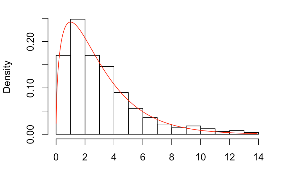
(a) ASE

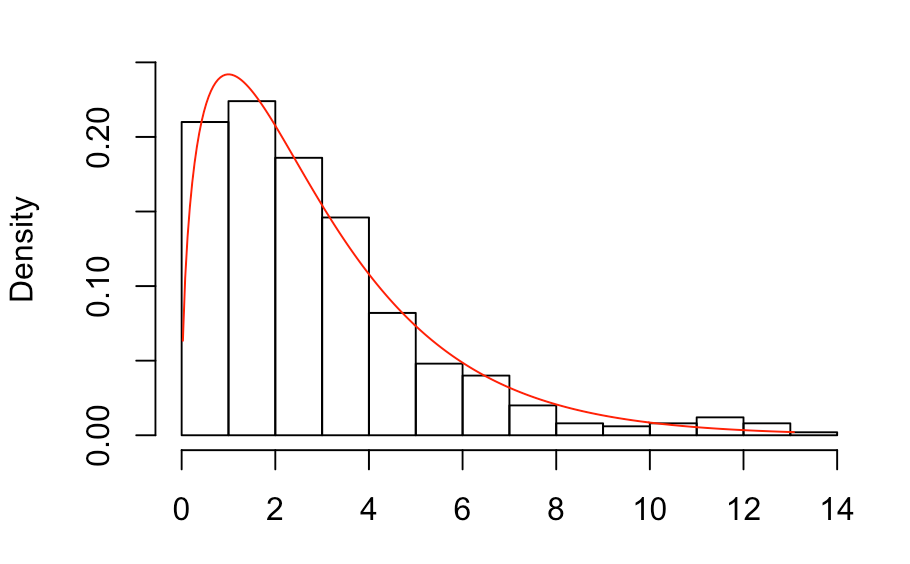
(b) LSE

Figure 1: Empirical histograms for the test statistics $T_{\mathrm{ASE}}$ and $T_{\mathrm{LSE}}$ under the null hypothesis when $\rho=1.0$. The setting is that of mixed-membership graphs on $n=3100$ vertices with parameters generated according to Model I. The red curve is the probability density function for the $\chi^{2}_{3}$ distribution.

We first generate graphs on $n=3100$ vertices according to the mixed membership SBM in Model I. Among these $3100$ vertices, $100$ vertices are assigned to have membership vector $\pi_{i}=(1-2cn^{-1/2},cn^{-1/2},cn^{-1/2})$ with $c=5$, and the remaining $3000$ vertices are equally assigned to the remaining membership vectors. The empirical size and power of the test statistics $T_{\mathrm{ASE}}$ and $T_{\mathrm{LSE}}$ for testing $\mathbb{H}_{0}\colon\pi_{i}=\pi_{j}$ against $\mathbb{H}_{A}\colon\pi_{i}\not=\pi_{j}$, under various choices of sparsity factors $\rho$, are reported in Table 2; the empirical size here refers to the null rejection rate. Table 2 also report the large-sample, theoretical power computed according to the non-central chi-square distribution with non-centrality parameters given in Theorem 3.2 and Theorem 4.1. We see that the empirical estimates of the power are almost identical to the true theoretical values. In addition, Figure 1 in Appendix A.1 plots the empirical histograms for $T_{\mathrm{ASE}}$ and $T_{\mathrm{LSE}}$ under the null hypothesis for $\rho=1.0$ and show that the distributions of $T_{\mathrm{ASE}}$ and $T_{\mathrm{LSE}}$ are well-approximated by the $\chi^{2}_{3}$ distribution.

Table 3: Empirical estimates for the size and power for the test statistics $G_{\mathrm{ASE}}$ and $G_{\mathrm{LSE}}$ for the degree-corrected mixed-membership stochastic block model graphs with various choices of degree heterogeneity parameter $k$. The alternative hypothesis corresponds to $\pi_{i}=(1,0,0)$ and $\pi_{j}=(1-10n^{-1/2},5n^{-1/2},5n^{-1/2})$. The rows with labels $\mathrm{ncp}$ are the non-centrality parameters $\mu$ for the local alternative hypothesis as $k$ changes.

$k$	1.3	1.4	1.5	1.6	1.7	1.8	1.9	2.0
Size ($G_{\mathrm{ASE}}$)	0.082	0.060	0.062	0.062	0.068	0.038	0.058	0.062
Size ($G_{\mathrm{LSE}}$)	0.088	0.062	0.058	0.060	0.072	0.038	0.060	0.056
Power ($G_{\mathrm{ASE}})$	0.472	0.566	0.602	0.592	0.672	0.668	0.768	0.824
Power ($G_{\mathrm{LSE}}$)	0.466	0.566	0.604	0.582	0.670	0.662	0.776	0.832
ncp ($G_{\mathrm{ASE}}$)	4.5332	5.3192	6.4099	6.4703	7.2737	6.7527	9.2965	11.6185
ncp ($G_{\mathrm{LSE}}$)	4.5607	5.3535	6.4497	6.5202	7.3236	6.8013	9.3074	11.5597
Theoretical Power ($G_{\mathrm{ASE}}$)	0.4634	0.5302	0.6144	0.6188	0.6734	0.6386	0.7848	0.8722
Theoretical Power ($G_{\mathrm{LSE}}$)	0.4658	0.5331	0.6173	0.6223	0.6766	0.6420	0.7853	0.8705

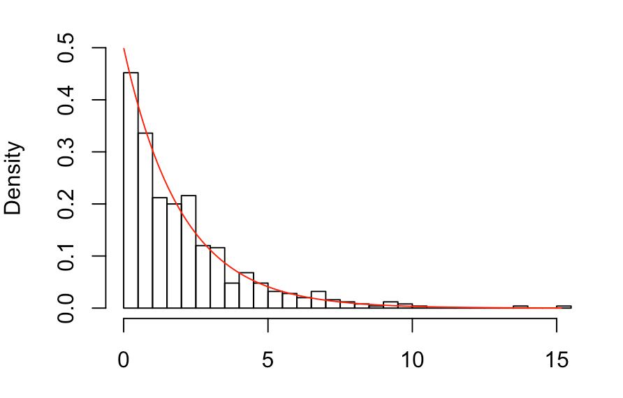
(a) ASE

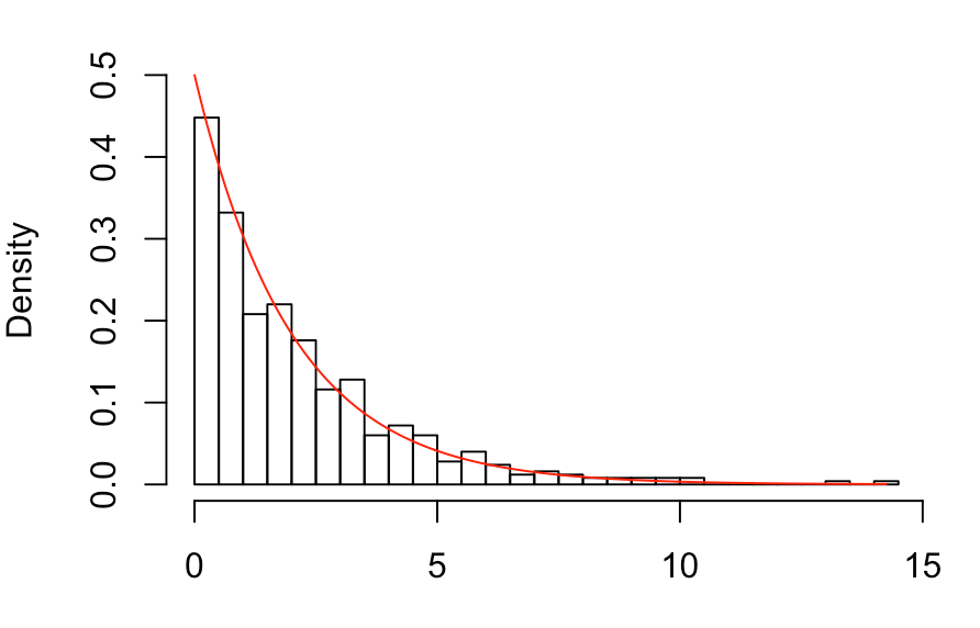
(b) LSE

Figure 2: Empirical histograms for the test statistics $G_{\mathrm{ASE}}$ and $G_{\mathrm{LSE}}$ under the null hypothesis when the degree heterogeneity coefficients are uniformly distributed in the interval $[1,2]$. The setting is that of degree-corrected mixed-membership graphs on $n=3100$ vertices with sparsity factor $\rho=0.25$ and parameters specified according to Model II. The red curve is the probability density function for the $\chi^{2}_{2}$ distribution.

We next generate graphs on $n=3100$ vertices according to the degree-corrected mixed membership SBM in Model II. Once again there are $100$ vertices assigned to have membership vectors $\pi_{i}=(1-2cn^{-1/2},cn^{-1/2},cn^{-1/2})$ with $c=5$ and the remaining $3000$ vertices are equally assigned to the remaining membership vectors. The empirical size and power of the test statistics $G_{\mathrm{ASE}}$ (Theorem 3.4) and $G_{\mathrm{LSE}}$ (Theorem C.1 in Appendix), for $\rho=0.25$ and various choices of $k\in\{1.3,1.4,\dots,2\}$, are reported in Table 3. Figure 2 in Appendix A.1 plots the empirical histograms for $G_{\mathrm{ASE}}$ and $G_{\mathrm{LSE}}$ under the null hypothesis when the degree heterogeneity parameters $\theta_{i}$ are uniformly distributed in the interval $[1,2]$ and the sparsity factor is $\rho=0.25$. Once again we see that the empirical estimates of the power are almost identical to the true theoretical values and furthermore the distributions of $G_{\mathrm{ASE}}$ and $G_{\mathrm{LSE}}$ are well-approximated by the $\chi^{2}_{2}$ distribution.

We also note that, in comparison to Table 2, Table 3 shows more deviation between the theoretical and empirical powers. We surmise that this is due to the additional variability in the latent positions of a degree-corrected SBM compared to those for a SBM (indeed, two nodes in the same community of a DCSBM can have quite different degrees profile). Estimation of the latent positions in a DCSBM is therefore generally less accurate than those for a SBM and thus we expect $G_{\mathrm{ASE}}$ (resp. $G_{\mathrm{LSE}}$) to converge to the limiting $\chi^{2}_{d-1}$ somewhat slower than the convergence of $T_{\mathrm{ASE}}$ (resp. $T_{\mathrm{LSE}}$) to $\chi^{2}_{d}$.

5.2 Model selection

We now examine how the previous test statistics can be used to choose between the stochastic block model and the degree-corrected stochastic block model. We perform $500$ Monte Carlo replicates where, in each replicate, we do the following steps.

1. Generate a $3$-blocks stochastic block model graph on $n=1500$ vertices, equal block sizes, and block probabilities matrix $\mathbf{B}=0.9\bm{1}\bm{1}^{\top}-0.6\mathbf{I}$.

2. Embed the graph into $\mathbb{R}^{3}$ using adjacency spectral embedding and then cluster these embedded vertices into $K=3$ communities.

3. Select $m=10$ pairs of nodes from each community and compute $T_{\mathrm{ASE}}$ for each pair.

4. Convert these test statistic values into $p$-values based on the quantiles of the $\chi^{2}_{3}$ distributions. Compute the test statistic $S_{1}$ as defined in Theorem 3.9 using these $p$-values.

5. Reject the null hypothesis that the graph is a $3$-blocks SBM graph if $S_{1}>\chi^{2}_{6,0.95}$, the $95$ percentile of the chi-square distribution with $6$ degrees of freedom.

We then perform another $500$ Monte Carlo replicates of the above steps, except that we now allow for degree heterogeneity by sampling, in addition to the above SBM parameters, a sequence of degree correction factors $\{\theta_{1},\theta_{2},\dots,\theta_{n}\}$ which are iid uniform random variables in the interval $[1,k]$ for $k\in\{1.3,1.4,\dots,2\}$. The number of times we reject the null hypothesis among the first and second batch of these $500$ replicates is an estimate of the significance level and power, respectively, for using $S_{1}$ as a goodness of fit test for deciding between a SBM and a degree-corrected SBM. Table 4 and Table 5 reported the empirical size and power for various values of $\rho\in\{0.3,0.4,\dots,1\}$ (under the null hypothesis) and $k\in\{1.3,1.4,\dots,2\}$ (under the alternative hypothesis), respectively. The results in Tables 4 and 5 indicate that the proposed model selection procedure frequently chooses the correct generative model for the observed graphs.

Table 4: Empirical estimates of the significance level for using $S_{1}$ as a goodness of fit test statistic for deciding between a stochastic block model and a degree-corrected stochastic block model.

$\rho$	0.3	0.4	0.5	0.6	0.7	0.8	0.9	1.0
Size	0.072	0.056	0.044	0.044	0.068	0.056	0.050	0.068

Table 5: Empirical estimates of the power for using $S_{1}$ as a goodness of fit test statistic for deciding between a stochastic block model and a degree-corrected stochastic block model.

$k$	1.3	1.4	1.5	1.6	1.7	1.8	1.9	2.0
Power	0.400	0.584	0.674	0.778	0.846	0.874	0.904	0.940

5.3 Power Comparison with Test Statistics in [17]

We discussed in Section 3.3 the relationship between our proposed test statistics and those studied in [17]; in particular the test statistics $T_{\mathrm{ASE}}$ and $\mathrm{G}_{\mathrm{ASE}}$ are asymptotically equivalent to those studied in [17]. We now conduct numerical simulations to compare the finite sample power of these test statistics under local alternatives. We used the same settings as those presented for Model I and Model II in Section 5.1, except that the block probabilities matrix $\mathbf{B}$ is now set to $\mathbf{B}=0.3\bm{1}\bm{1}^{\top}+0.6\mathbf{I}$. We chose this $\mathbf{B}$ because the theoretical results in [17] require $\mathbf{B}$ to be positive-semidefinite. The results are presented in Table 6 and Table 7. Table 6 indicates that, for the Model I setting, the (empirical) powers for all test statistics are almost identical. In contrast, Table 7 shows discernible differences between these test statistics for Model II. In particular our test statistics have higher (finite-sample) power compared to those of [17]; these difference are statistically significant (confirmed via McNemar’s test [37]).

Table 6: Empirical estimates for the power of the test statistics $T_{\mathrm{FAN}}$, $T_{\mathrm{ASE}}$ and $T_{\mathrm{LSE}}$ for mixed membership stochastic block model graphs under local alternative hypothesis corresponding to $\pi_{i}=(1,0,0)$ and $\pi_{j}=(1-10n^{-1/2},5n^{-1/2},5n^{-1/2})$ with various choices of sparsity parameter $\rho$. The estimates are based on $500$ Monte Carlo replicates.

$\rho$	0.1	0.2	0.3	0.4	0.5	0.6	0.7	0.8	0.9	1.0
Power ($T_{\mathrm{FAN}}$)	0.270	0.328	0.450	0.570	0.696	0.770	0.906	0.954	0.988	1
Power ($T_{\mathrm{ASE}}$)	0.280	0.322	0.448	0.564	0.696	0.776	0.906	0.954	0.988	1
Power ($T_{\mathrm{LSE}}$)	0.292	0.328	0.448	0.564	0.702	0.780	0.910	0.954	0.990	1

Table 7: Empirical estimates for the power of the test statistics $G_{\mathrm{FAN}}$, $G_{\mathrm{ASE}}$ and $G_{\mathrm{LSE}}$ for degree-corrected mixed membership stochastic block model graphs under local alternative hypothesis corresponding to $\pi_{i}=(1,0,0)$ and $\pi_{j}=(1-10n^{-1/2},5n^{-1/2},5n^{-1/2})$ with various choices of degree heterogeneity parameter $k$. The estimates are based on $500$ Monte Carlo replicates.

$k$	1.1	1.2	1.3	1.4	1.5	1.6	1.7	1.8	1.9	2.0
Power ($G_{\mathrm{FAN}}$)	0.304	0.356	0.430	0.414	0.452	0.564	0.642	0.640	0.444	0.834
Power ($G_{\mathrm{ASE}}$)	0.356	0.404	0.466	0.452	0.484	0.594	0.664	0.678	0.480	0.840
Power ($G_{\mathrm{LSE}}$)	0.354	0.408	0.470	0.456	0.504	0.592	0.678	0.666	0.492	0.838

6 Real Data Analysis

6.1 U.S. Political Blogs data

We now analyze a network of U.S. Political Blogs as compiled in [2]. This directed network contains snapshots of 1494 web blogs on US politics recorded in 2005. Each blog is represented by a node and a (directed) link between two nodes indicates the presence of a hyperlink between them. Blogs are labelled as being either liberal or conservative by self-reported or automated categorizations or by manually looking at the incoming and outgoing links and posts of each blog around the time of the 2004 presidential election. While the resulting labels are not $100\%$ exact, they are still reasonably accurate and will serve as the assumed ground truth for the current analysis.

We first consider its undirected version. We do some pre-processing on the data, namely (1) we keep only the largest connected component (2) we convert directed edges to be undirected and (3) we remove all multi-edges and loops. We then embed the resulting network into $a=d=2$ dimensions. The choice of $a=d=2$ is determined by looking at a scree plot of the eigenvalues. We then apply the test statistics in Section 3 and Section 4 to test the hypothesis that a given pair of nodes have the same latent positions. Due to the large number of possible pairs of nodes, we randomly choose 1000 pairs of nodes within the same community and 1000 pairs in different communities to perform our test. The resulting sensitivity and specificity are reported in Table 8. Once again, the threshold for classifying a pair of vertices as having the same latent positions is based on the $95\%$ percentile of the chi-square distribution with the appropriate degrees of freedom. Table 8 indicates that $T_{\mathrm{ASE}}$ and $G_{\mathrm{ASE}}$ perform reasonably well; nevertheless $G_{\mathrm{ASE}}$ is preferable to $T_{\mathrm{ASE}}$ as it has both high sensitivity and high specificity.

Table 8: Sensitivity and specificity of different test statistics for the U.S. Political Blogs data. The threshold for classifying a pair of vertices as having the same latent positions is based on the $95\%$ percentile of the $\chi^{2}_{2}$ distribution (for $T_{\mathrm{ASE}}$ and $T_{\mathrm{LSE}}$) and $\chi^{2}_{1}$ distribution (for $G_{\mathrm{ASE}}$ and $G_{\mathrm{LSE}}$).

	$T_{\mathrm{ASE}}$	$T_{\mathrm{LSE}}$	$G_{\mathrm{ASE}}$	$G_{\mathrm{LSE}}$
Sensitivity	0.839	0.643	0.653	0.007
Specificity	0.335	0.354	0.749	0.989

The sensitivity and specificity values for $G_{\mathrm{ASE}}$ suggests that a degree corrected SBM is a better model than a vanilla SBM for this political blogs network. We verify this hypothesis by performing the model selection procedure discussed in Section 3.4. More specifically we embed the graph into $\mathbb{R}^{2}$ using adjacency spectral embedding and then cluster these embedded vertices into $K=2$ communities. We then select $m=10$ pairs of nodes from each cluster and apply the test statistic $T_{\mathrm{ASE}}$ to each of these pairs and get the $p$-values. Then the test statistic $S_{1}$ as defined in Theorem 3.9 is computed using these $p$-values. We repeat the above procedure $1000$ times, each time choosing a different random set of $m=10$ pairs of nodes from each cluster. Among these 1000 Monte Carlo replicates, we reject the null hypothesis that the stochastic block model is a proper fit for the political blogs network more than 600 times. On the other hand, if we set the degree-corrected model as the null model and repeat the above procedure except that we use $G_{\mathrm{ASE}}$ instead of $T_{\mathrm{ASE}}$ to get the $p$-values, we find that we reject the null hypothesis less than $100$ times. We thus conclude that the degree-corrected SBM is a more appropriate model for the political blogs. This conclusion is consistent with earlier findings in [13, 28, 54].

To further illustrate our test statistics, we randomly select 5 blogs each from the top 20 liberal and top 20 conservative blogs as indicated in [2]. The information of these 10 blogs are presented in Table 9. We apply $G_{\mathrm{ASE}}$ to each pair of nodes and the resulting $p$-values are reported in Table 10. Table 10 indicates that our test statistic is highly accurate for predicting whether or not two blogs are similarly labelled. For instance, blog $1$ and blog $2$ in Table 9 are both labelled as “conservative” and the $p$-value of our test statistic is close to $1$. Similarly, blogs $3$ and $7$ have different labels and the $p$-value of our test statistic is now almost $0$. Note however, that there are a few $p$-values that are possibly unexpected. For example the $p$-values for blog $5$ and blog $3$ are quite small and the $p$-values for blog $5$ and blog $1$ are also quite small, even though these three blogs are all “conservative” blogs. One possible explanation is that blog $5$ is an aggregate blog and thus was written by multiple authors with possibly different political leanings. Similarly, the $p$-values between blog $6$ and other liberal blogs are also small, and this may be due to the fact that blog $6$ has a substantially high proportion of links to conservative blogs.

Table 9: 5 of the top 20 conservative blogs and 5 of the top 20 liberal blogs. The two right columns show for comparison how many conservative and liberal blogs from the larger set linked to the blog in February 2005.

ID	Weblog	Label	# links to conservative blogs	# links to liberal blogs
1	timblair.spleenville.com	Conservative	80	7
2	windsofchange.net	Conservative	65	16
3	vodkapundit.com	Conservative	97	9
4	rogerlsimon.com	Conservative	74	6
5	deanesmay.com	Conservative	79	8
6	wonkette.com	Liberal	30	83
7	j-bradford-delong.net/movable_type	Liberal	11	98
8	prospect.org/weblog	Liberal	11	102
9	americablog.blogspot.com	Liberal	5	64
10	jameswolcott.com	Liberal	6	74

Table 10: $p$-values based on the test statistic $G_{\mathrm{ASE}}$ for selected blogs in Table 9.

ID	1	2	3	4	5	6	7	8	9	10
1	1.000	0.811	0.702	0.263	0.024	0.000	0.000	0.000	0.000	0.000
2	0.811	1.000	0.882	0.298	0.013	0.000	0.000	0.000	0.000	0.000
3	0.702	0.882	1.000	0.303	0.005	0.000	0.000	0.000	0.000	0.000
4	0.263	0.298	0.303	1.000	0.091	0.000	0.000	0.000	0.000	0.000
5	0.024	0.013	0.005	0.091	1.000	0.000	0.000	0.000	0.000	0.000
6	0.000	0.000	0.000	0.000	0.000	1.000	0.001	0.001	0.001	0.000
7	0.000	0.000	0.000	0.000	0.000	0.001	1.000	0.830	0.300	0.077
8	0.000	0.000	0.000	0.000	0.000	0.001	0.830	1.000	0.364	0.087
9	0.000	0.000	0.000	0.000	0.000	0.001	0.300	0.364	1.000	0.522
10	0.000	0.000	0.000	0.000	0.000	0.000	0.077	0.087	0.522	1.000

Finally we also analyze the political blogs networks as a directed network using the test statistics described in Appendix E.1. More specifically we keep only the largest connected component, remove all multi-edges and loops, but keep the orientation of the directed edges. We embed the resulting directed graph into $\mathbb{R}^{2}$; we chose $d=2$ to be consistent with the above analysis of the undirected case. Using this embedding, we test the null hypothesis that two nodes have the same outgoing latent positions up to scaling. Our rationale for looking only at the outgoing latent positions is that the author of a blog can control the outgoing links (from their blog to other blogs) but cannot control the incoming links. We apply $G_{\mathrm{out}}$ which is the degree-corrected version of $T_{\mathrm{out}}$ mentioned in Remark E.1. Once again, due to the large number of possible pairs of nodes, we randomly choose 1000 pairs of nodes within the same community and 1000 pairs in different communities to perform our test. We use the $95\%$ percentile of the $\chi^{2}_{1}$ distribution as the threshold for classifying two blogs to be from the same community. The resulting sensitivity and specificity are then $0.43$ and $0.92$, respectively. The pairwise $p$-values between the $10$ selected blogs are presented in Table 11; once again we can predict quite accurately whether or not two blogs are similarly labelled.

Table 11: $p$-values based on the test statistic $G_{\mathrm{out}}$ for selected blogs in Table 9.

ID	1	2	3	4	5	6	7	8	9	10
1	1.0000	0.8301	0.1460	0.9314	0.1587	0.0014	0.0017	0.0000	0.0000	0.0404
2	0.8301	1.0000	0.0946	0.8848	0.2231	0.0011	0.0017	0.0000	0.0000	0.0406
3	0.1460	0.0946	1.0000	0.1090	0.0334	0.0065	0.0019	0.0000	0.0000	0.0396
4	0.9314	0.8848	0.1090	1.0000	0.1446	0.0011	0.0016	0.0000	0.0000	0.0399
5	0.1587	0.2231	0.0334	0.1446	1.0000	0.0002	0.0013	0.0000	0.0000	0.0400
6	0.0014	0.0011	0.0065	0.0011	0.0002	1.0000	0.0608	0.0487	0.0168	0.0861
7	0.0017	0.0017	0.0019	0.0016	0.0013	0.0608	1.0000	0.4952	0.8831	0.5430
8	0.0000	0.0000	0.0000	0.0000	0.0000	0.0487	0.4952	1.0000	0.2994	0.2005
9	0.0000	0.0000	0.0000	0.0000	0.0000	0.0168	0.8831	0.2994	1.0000	0.5311
10	0.0404	0.0406	0.0396	0.0399	0.0400	0.0861	0.5430	0.2005	0.5311	1.0000

6.2 Leeds Butterfly Dataset

We consider in this section the problem of testing for equality of community assignments in Popularity Adjusted Block Models (PABM) and apply the resulting test statistic to the Leeds Butterfly dataset of [52]. We start by describing the PABM proposed in [45]. Let $K\geq 1$ be an integer and let $\bm{\Lambda}$ be a $n\times K$ matrix whose entries $\lambda_{ik}\in[0,1]$ for all $i\in\{1,2,\dots,n\}$ and $k\in\{1,2,\dots,K\}$. Let $\tau=(\tau_{1},\ldots,\tau_{n})\in\{1,\ldots,K\}^{n}$ be the community assignments where $\tau_{i}=k$ if node $i$ belongs to community $k$. A graph $G$ with adjacency matrix $\mathbf{A}$ is said to be a popularity adjusted block model (PABM) with $K$ communities, popularity vectors $\mathbf{\Lambda}$, and sparsity parameter $\rho_{n}$ if the $\mathbf{A}_{ij}$’s are independent Bernoulli variables satisfying

$$P(\mathbf{A}_{ij}=1)=\mathbf{P}_{ij}=\rho_{n}\lambda_{i\tau_{j}}\lambda_{j\tau_{i}}$$

The entries $\lambda_{ik}$ represents the popularity of node $i$ in community $k$; that is to say, larger values of $\lambda_{ik}$ are associated with more edges between node $i$ and other nodes in community $k$.

The motivation for the PABM model is as follows. Recall that the degree-corrected SBM (DCSBM) is a generalization of the SBM and allows for heterogeneous degrees for nodes in the same community. A PABM also allows for degree heterogeneity of nodes from the same community, but this heterogeneity is more flexible than that of a DCSBM. More specifically, suppose $i$ and $j$ are two nodes assigned to the same community in a PABM. Then it is possible that node $i$ is more likely than node $j$ to connect with nodes in some community $k$ (so that $\lambda_{ik}>\lambda_{jk}$), while node $j$ is more likely than node $i$ to connect with nodes in some other community $\ell\not=k$ (so that $\lambda_{j\ell}>\lambda_{i\ell}$). Now suppose that $i$ and $j$ belong to the same community in a degree-corrected SBM. Then as $i$ and $j$ are associated with (scalar-valued) degree correction factors $\theta_{i}$ and $\theta_{j}$, if $\theta_{i}>\theta_{j}$ then node $i$ is more likely than node $j$ to connect with any arbitrary node $v$. In other words, if a given node $i$ is more popular than node $j$ in some community $k$, then $i$ is also more popular than $j$ in all community $\ell\not=k$.

A PABM is also a special case of a GRDPG. More specifically, assume without loss of generality that the rows of $\bm{\Lambda}$ are arranged in increasing order of the community assignment $\tau$, i.e., if $i<j$ then $\tau_{i}\leq\tau_{j}$. Denote the $i$th row of $\bm{\Lambda}$ as $\lambda_{i}$. Now let $\bm{\Lambda}^{(k)}$ be the submatrix of $\bm{\Lambda}$ obtained by keeping only the $\lambda_{i}$’s for which $\tau_{i}=k$. A PABM graph with parameters $\bm{\Lambda}$ given above is equivalent to a GRPDG with signatures $a=K(K+1)/2$ and $b=K(K-1)/2$, and latent positions matrix $\mathbf{X}$ given by $\mathbf{X}=\bm{\Lambda}^{(1)}\oplus\bm{\Lambda}^{(2)}\oplus\cdots\oplus\bm{\Lambda}^{(K)}$; here $\oplus$ denote the direct sum for matrices, i.e., $\mathbf{M}_{1}\oplus\mathbf{M}_{2}$ is the block matrix of the form $\Bigl{(}\begin{smallmatrix}\mathbf{M}_{1}&\bm{0}\\ \bm{0}&\mathbf{M}_{2}\end{smallmatrix}\Bigr{)}$. The above structure for $\mathbf{X}$ implies that the $K$ communities of a PABM correspond to $K$ mutually orthogonal subspaces in $\mathbb{R}^{K^{2}}$. See Theorem 1 and Theorem 2 in [29] for more details.

Given two nodes $i$ and $j$ in a PABM we can test the hypothesis that they have the same latent positions, possibly up to scaling, by using the test statistics provided in Section 3 and Section 4. However, if our main interest is in testing whether or not two given nodes $i$ and $j$ belong to the same community in a PABM then the above test statistics no longer apply. Indeed, in contrast to the SBM or DCSBM where there exists a $1$-to-$1$ correspondence between the community assignments $\tau_{i}$ and the point masses $\nu_{\tau_{i}}$ (see Remark 2.2), two nodes from the same community in a PABM can have drastically different latent positions.

Let $U_{i}$ denote the $i$th row of the matrix $\mathbf{U}$ where $\mathbf{U}\mathbf{S}\mathbf{U}^{\top}$ is the eigen-decomposition of $\mathbf{P}$. Theorem 2 of [29] show that $U_{i}^{\top}U_{j}=0$ if and only if node $i$ and $j$ belong to different communities. Leveraging this fact we propose a test statistic for testing $\tau_{i}=\tau_{j}$ but, unlike the test procedures in Section 3 and Section 4, the null hypothesis now is that two node $i$ and node $j$ belong to different communities i.e., we are interested in testing the hypothesis

$$\mathbb{H}_{0}\colon\tau_{i}\neq\tau_{j}\quad\text{against}\quad\mathbb{H}_{A}\colon\tau_{i}=\tau_{j}$$ (25)

We then have the following result.

Theorem 6.1.

Let $\mathbf{A}$ be a graph on $n$ vertices generated from a PABM with $K$ communities and sparsity factor $\rho_{n}$. Let $\hat{\mathbf{X}}$ be the adjacency spectral embedding of $\mathbf{A}$ into $\mathbb{R}^{K^{2}}$. Define the test statistic

$$T_{\mathrm{PABM}}(\hat{U}_{i},\hat{U}_{j})=\frac{n\rho_{n}^{1/2}\hat{U}_{i}^{\top}\hat{U}_{j}}{\bigl{(}\hat{U}_{i}^{\top}\hat{\bm{\Sigma}}(\hat{U}_{j})\hat{U}_{i}+\hat{U}_{j}^{\top}\hat{\bm{\Sigma}}(\hat{U}_{i})\hat{U}_{j}\bigr{)}^{1/2}}$$

where $\hat{\bm{\Sigma}}(\hat{U}_{i})$ and $\hat{\bm{\Sigma}}(\hat{U}_{j})$ are as defined in Corollary 3.6, with $a=K(K+1)/2$ and $b=K(K-1)/2$. Then under the null hypothesis $\mathbb{H}_{0}\colon\tau_{i}\neq\tau_{j}$ and for $n\rightarrow\infty$ with $n\rho_{n}=\omega(\log n)$, we have

$$T_{\mathrm{PABM}}(\hat{U}_{i},\hat{U}_{j})\rightsquigarrow\mathcal{N}(0,1)$$

The above result indicates that, for a given significance level $\alpha$, we reject $\mathbb{H}_{0}$ if $|T_{\mathrm{PABM}}(\hat{U}_{i},\hat{U}_{j})|>Z_{1-\alpha/2}$ where $Z_{1-\alpha/2}$ is the $100\times(1-\alpha/2)$ th percentile of $\mathcal{N}(0,1)$. Simulation results for Theorem 6.1 are provided in Section A.2 of the appendix.

We now apply the proposed test statistic to the Leeds Butterfly dataset of [52]. This dataset contains similarity measurements between $832$ butterfly images; these images are labeled into $10$ different classes. Following [40], we select a subset of $373$ images corresponding to the $K=4$ largest classes and form an adjacency matrix by thresholding these pairwise similarities so that each image is mapped to a vertex and two vertices are connected if their similarity measure is positive. The resulting (undirected) graph has $20566$ edges. We use $T_{\mathrm{PABM}}$ to test, for each of the $\tbinom{373}{2}$ pairs of nodes, the hypothesis in Eq. (25). Choosing the $95\%$ of the standard normal distribution as a threshold, we achieve a specificity of $0.93$ and sensitivity of $0.67$.

7 Discussion

In this paper we developed Mahalanobis distance based test statistics to determine whether or not two vertices have the same latent positions, or the same latent positions up to scaling (in the degree-corrected case). We established limiting chi-square distributions for the test statistics under both the null and local alternative hypothesis; furthermore, our expressions for the non-centrality parameters under the local alternative are invariant with respect to the non-identifiability of the latent positions. Leveraging these limit results, we also propose test statistics for deciding between the standard stochastic block model (SBM) and a degree-corrected stochastic block model (DCSBM), and choosing between the Erdős–Rényi model and stochastic block model.

We note that the values of the non-centrality parameters for $T_{\mathrm{ASE}}$ and $T_{\mathrm{LSE}}$ in Table 2 are almost identical; similarly, the values of the non-centrality parameters for $G_{\mathrm{ASE}}$ and $G_{\mathrm{LSE}}$ in Table 3 are also almost identical. This suggests that the test statistics constructed using the different embeddings are, asymptotically, almost equivalent. Indeed, we were not able to find simulation settings for which either the non-centrality parameters of $T_{\mathrm{ASE}}$ and $T_{\mathrm{LSE}}$, or the non-centrality parameters of $G_{\mathrm{ASE}}$ and $G_{\mathrm{LSE}}$, are well separated. Nevertheless, for the real data analysis in Section 6, the test statistics associated with different embeddings do have significantly different error rates. A more precise understanding of why these differences arise is therefore of some practical interests.

Finally, as we allude to in the introduction, a GRDPG is a special case of a latent position graph. It is thus natural to pose the question of testing the hypothesis $\mathbb{H}_{0}\colon X_{i}=X_{j}$ for general latent position graphs, and in particular to study test statistics based on the Mahalanobis distance between the rows of the embeddings as is done in the current paper. This problem is, however, highly non-trivial. Indeed, the edge probabilities matrix of a latent position graph is generally not low-rank; in contrast, limit results for spectral embeddings for random graphs, such as those in [16, 44], almost always assume that the edge probabilities matrix is low-rank. Theoretical results for testing $\mathbb{H}_{0}\colon X_{i}=X_{j}$ in general latent position graphs require new and far-reaching extensions of existing results for spectral embeddings.

Appendix A Additional Numerical Experiments

A.1 Additional Plots

A.2 Hypothesis Testing in PABM

In this section, we conduct simulations to investigate the finite sample performance of $T_{\mathrm{PABM}}$ proposed in Section 6.2. We generate graphs from PABM on $n=4800$ vertices with $K=2,3,4,5$. For each choice of $K$, $n$ vertices are equally assigned to the $K$ different communities. Then $\{\lambda^{(k\ell)}\}_{K}$ are generated according to the assigned community labels. Here $\{\lambda^{(k\ell)}\}_{K}$ are parameters of another view of PABM specified in [29]. Specifically, we have within-group popularities $\lambda^{(kk)}\stackrel{{\scriptstyle\text{ iid }}}{{\sim}}\operatorname{Beta}(2,1)$ and between-group popularities $\lambda^{(k\ell)}\stackrel{{\scriptstyle\text{ iid }}}{{\sim}}\operatorname{Beta}(1,2)$ for $k\neq\ell$. $\mathbf{P}$ is constructed using the drawn $\{\lambda^{(k\ell)}\}_{K}$, and $\mathbf{A}$ is drawn from $\mathbf{P}$. We do $500$ Monte Carlo replicates for each choice of $K$ and $\alpha$ is set to be $0.05$. The empirical histograms under the null hypothesis and empirical sizes and powers are presented below in Figure 3 and Table 12. We see from Figure 3 that the distributions of $T_{ij}$ are well-approximated by the standard normal distribution. The relatively large size and small power when $K=5$ might be due to the fact that we need larger sample size to ensure the finite sample convergence when the model becomes more complex.

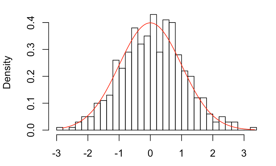
(a) $K=2$

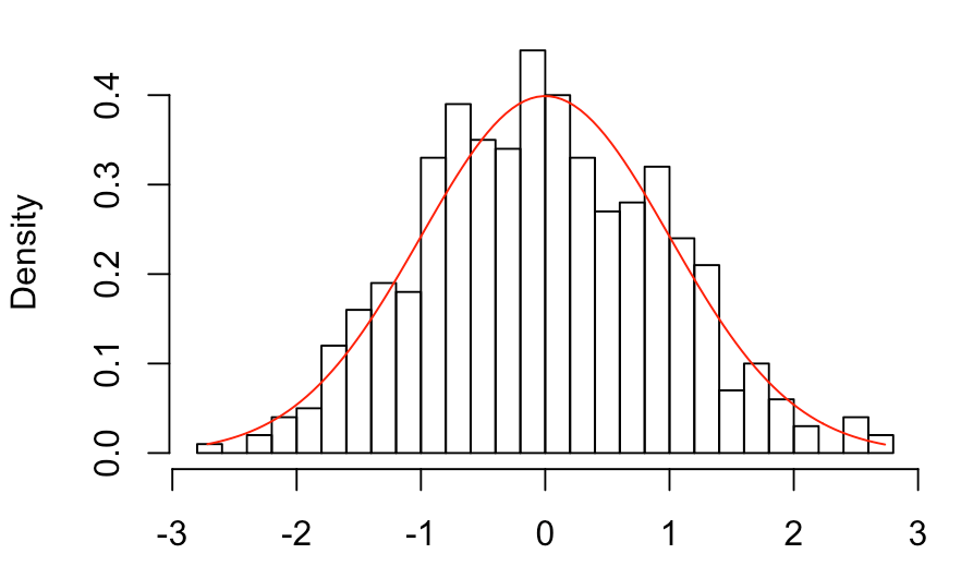
(b) $K=3$

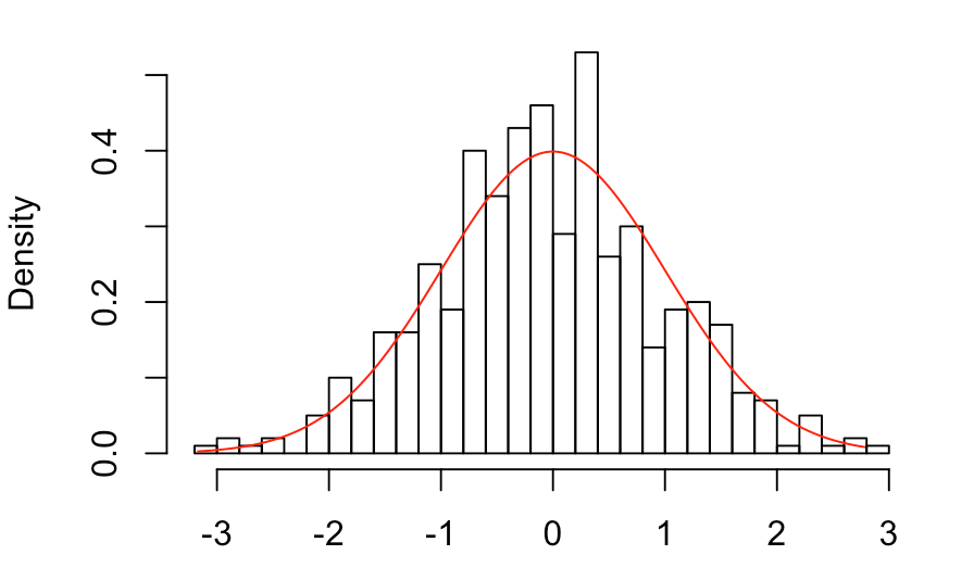
(c) $K=4$

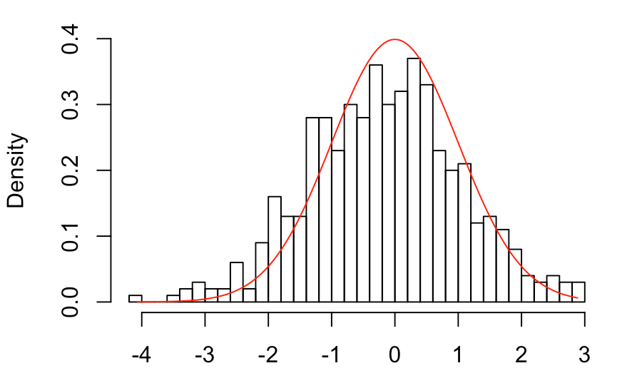
(d) $K=5$

Figure 3: Empirical histograms for the test statistic $T_{\mathrm{PABM}}$ under the null hypothesis when $n=4800$ and $K=2,3,4,5$. The setting is that of PABM graphs on $n=4800$ vertices with $K$ communities. The red curve is the probability density function for the standard normal distribution.

Table 12: Empirical sizes for the test statistic under the null hypothesis when $n=4800$ and $K=2,3,4,5$.

$K$	$2$	$3$	$4$	$5$
Size	0.052	0.034	0.046	0.086
Power	1	1	1	0.81

A.3 American Football data

Table 13: Sensitivity and specificity of different test statistics for the American College Football data. The threshold for classifying a pair of vertices as having the same latent positions is based on the $95\%$ percentile of the $\chi^{2}_{4}$ distribution (for $T_{\mathrm{ASE}}$ and $T_{\mathrm{LSE}}$) and $\chi^{2}_{3}$ distribution (for $G_{\mathrm{ASE}}$ and $G_{\mathrm{LSE}}$).

	$T_{\mathrm{ASE}}$	$T_{\mathrm{LSE}}$	$G_{\mathrm{ASE}}$	$G_{\mathrm{LSE}}$
Sensitivity	0.828	0.486	0.585	0.578
Specificity	0.973	0.952	0.942	0.934

We now examine a network based on the American College Football data as considered in [23]. This network is a representation of games between Division IA colleges during the regular season of Fall 2000. Vertices represent teams and two teams are connected by an edge whenever there is a game played between these teams. There are 115 vertices and 616 edges. These 115 teams are divided into 12 conferences, each with 5-12 members, and each conference serves as a community/block. Games are more frequent between teams in the same conference compared to teams in different conferences. In addition, games between teams from different conferences are more frequent if these teams are geographically close to each other. For this network we choose the embedding dimension as $d=4$ by looking at a scree plot of the eigenvalues, and among these $d=4$ eigenvalues, all of them are positive and thus we set $a=4$ and $b=0$. We apply all four test statistics we propose to each pair of nodes and compute the sensitivity and specificity for each test statistic for testing the hypothesis that two vertices belong to the same community. These values are reported in Table 13; the threshold for classifying a pair of vertices as having the same latent positions is based on the $95\%$ percentile of the $\chi^{2}_{4}$ distribution (for $T_{\mathrm{ASE}}$ and $T_{\mathrm{LSE}}$) and $\chi^{2}_{3}$ distribution (for $G_{\mathrm{ASE}}$ and $G_{\mathrm{LSE}}$). Note that the number of “true positives” and “true negatives” are quite unbalanced as, among the $\tbinom{115}{2}$ different pairs of nodes, there are $517$ pairs of nodes belonging to the same community and $6038$ pairs of nodes belonging to different communities. We also plot, in Figure 4, the ROC curves and the resulting AUCs for different choices of the test statistics. These ROC curves are obtained by considering the values of a test statistic as values of a “score” function, and “classifying” a given pair of vertices as being labeled “$+1$” or “$-1$” depending on whether or not the “score” exceeds some threshold. Figure 4 indicates that the AUC of $0.925$ for $T_{\mathrm{ASE}}$ is much higher compared to the remaining test statistics, and that $T_{\mathrm{ASE}}$ performs well in terms of both the sensitivity and specificity. In other words, by using $T_{\mathrm{ASE}}$, we are able to correctly infer the membership relationships between almost all pair of nodes. The incorrectness might come from the nonuniform pattern of games between different conferences and small sample size.

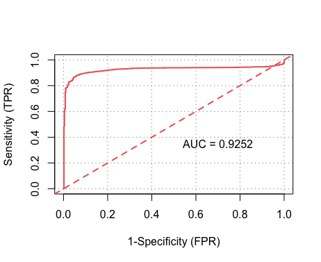
(a) $T_{\mathrm{ASE}}$

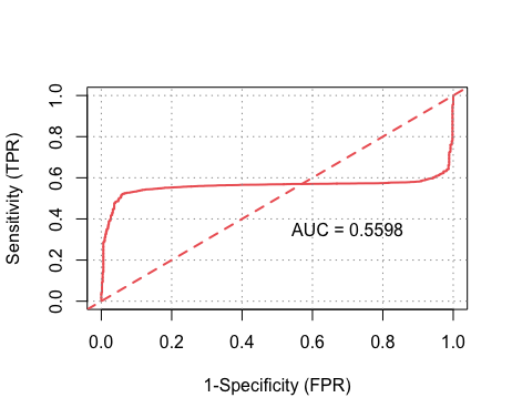
(b) $T_{\mathrm{LSE}}$

(c) $G_{\mathrm{ASE}}$

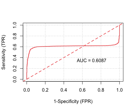
(d) $G_{\mathrm{LSE}}$

Figure 4: ROC curves and their corresponding AUC for the American College Football data.

Appendix B Non-identifiability of latent positions for GRDPG

We now provide a simple example for why the representation $\mathbf{Z}=\mathbf{U}|\mathbf{S}|^{1/2}$ obtained from the eigendecomposition of the edge probability matrix $\mathbf{P}$ is generally not suitable for generating $\mathbf{P}$.

Consider a mixed membership stochastic block model with block probabilities matrix

$$\mathbf{B}=0.4\bm{1}\bm{1}^{\top}-0.2\mathbf{I}=\begin{bmatrix}0.2&0.4&0.4\\ 0.4&0.2&0.4\\ 0.4&0.4&0.2\end{bmatrix}.$$

The matrix $\mathbf{B}$ induces a generalized random dot product graph with signature $a=1$ and $b=2$. Let $v_{1},v_{2},v_{3}$ be the vectors in $\mathbb{R}^{3}$ given by

$$v_{1}\approx(-0.577,0.365,0),\quad v_{2}\approx(-0.577,-0.182,-0.316),\quad v_{3}\approx(-0.577,-0.182,0.316).$$

The $\{v_{1},v_{2},v_{3}\}$ are the latent positions generating the block probabilities matrix $\mathbf{B}$, i.e., $v_{i}^{\top}\mathbf{I}_{1,2}v_{i}=0.2$ for all $i$ and $v_{i}^{\top}\mathbf{I}_{1,2}v_{j}=0.4$ for all $j\not=i$. Now given any node $i$ with mixed membership vector $\pi_{i}=(\pi_{i1},\pi_{i2},\pi_{i3})$, we can assign to $i$ the latent position representation $X_{i}=\sum_{j}\pi_{ij}v_{j}$. Next consider two mixed membership SBM graphs on $4$ vertices with $\pi_{1}=(1,0,0),\pi_{2}=(0,1,0)$, and $\pi_{3}=(0,0,1)$ for both graphs, $\pi_{4}=(0.25,0.25,0.5)$ for the first graph and $\pi_{4}=(0.2,0.6,0.2)$ for the second graph. Let $\mathbf{P}^{(1)}$ and $\mathbf{P}^{(2)}$ be the edge probabilities matrix for these graphs and let $\mathbf{Z}^{(1)}$ and $\mathbf{Z}^{(2)}$ be the representations obtained from the eigendecompositions of $\mathbf{P}^{(1)}$ and $\mathbf{P}^{(2)}$. The first three rows of $\mathbf{Z}^{(1)}$ and $\mathbf{Z}^{(2)}$ correspond to the same vertices; in particular the second and third row of $\mathbf{Z}^{(1)}$ and $\mathbf{Z}^{(2)}$ are the vertices with $\pi_{2}=(0,1,0)$ and $\pi_{3}=(0,0,1)$. We expect their representations to be identical in $\mathbf{Z}^{(1)}$ and $\mathbf{Z}^{(2)}$. This is, however, not the case; the eigendecomposition of $\mathbf{P}^{(1)}$ and $\mathbf{P}^{(2)}$ using R yields

$$Z^{(1)}_{2}=(-0.584,-0.202,-0.316),\,\,\|Z^{(1)}_{2}\|\approx 0.69,\quad Z^{(2)}_{2}=(-0.558,0.334,0),\,\,\|Z^{(2)}_{2}\|\approx 0.65,$$

$$Z^{(1)}_{3}=(-0.565,0.346,0),\,\,\|Z^{(1)}_{3}\|\approx 0.66,\quad Z^{(2)}_{3}\approx(-0.588,-0.214,0.316),\,\,\|Z^{(2)}_{3}\|\approx 0.70.$$

Here $Z^{(k)}_{i}$ denote the $i$th row of $\mathbf{Z}^{(k)}$ and $\|\cdot\|$ denote the $\ell_{2}$ norm of a vector. As $\|Z^{(1)}_{2}\|\not=\|Z^{(2)}_{2}\|$ and $\|Z^{(1)}_{3}\|\not=\|Z^{(2)}_{3}\|$, these representations cannot be aligned using orthogonal transformations. In summary, by changing the mixed membership vector of a single vertex $\pi_{4}$ we also change the latent vectors representation of the remaining vertices in $\mathbf{Z}^{(1)}$ and $\mathbf{Z}^{(2)}$.

Proofs of Proposition 2.3 and Proposition 2.5

We first prove Proposition 2.3. Let $\mathbf{X}$ and $\mathbf{Y}$ be $n\times d$ matrices of full-column ranks. Then both $\mathbf{X}^{\top}\mathbf{X}$ and $\mathbf{Y}^{\top}\mathbf{Y}$ are invertible. The condition $\mathbf{X}\mathbf{I}_{a,b}\mathbf{X}^{\top}=\mathbf{Y}\mathbf{I}_{a,b}\mathbf{Y}^{\top}$ then implies

$$\mathbf{X}=\mathbf{Y}\mathbf{I}_{a,b}\mathbf{Y}^{\top}\mathbf{X}(\mathbf{X}^{\top}\mathbf{X})^{-1}\mathbf{I}_{a,b}.$$

Now let $\mathbf{Q}=\mathbf{I}_{a,b}\mathbf{Y}^{\top}\mathbf{X}(\mathbf{X}^{\top}\mathbf{X})^{-1}\mathbf{I}_{a,b}$. We then have

$$\mathbf{Q}^{\top}\mathbf{I}_{a,b}\mathbf{Q}=\mathbf{I}_{a,b}(\mathbf{X}^{\top}\mathbf{X})^{-1}\mathbf{X}^{\top}\mathbf{Y}\mathbf{I}_{a,b}\mathbf{Y}^{\top}\mathbf{X}(\mathbf{X}^{\top}\mathbf{X})^{-1}\mathbf{I}_{a,b}=\mathbf{I}_{a,b}$$

and hence $\mathbf{Q}^{\top}$ is an indefinite orthogonal matrix. Therefore $\mathbf{Q}$ is also indefinite orthogonal, and Proposition 2.3 is established.

We now prove Proposition 2.5. We will prove a stronger result in that $\|\mathbf{Z}\|_{*}\leq\|\mathbf{X}\|_{*}$ for any unitarily invariant $Q$-norm $\|\cdot\|_{*}$. A norm $\|\cdot\|_{*}$ is said to be a $Q$-norm if there exists a unitarily invariant norm $\|\cdot\|_{\mathrm{UI}}$ such that $\|\mathbf{M}\|_{*}^{2}=\|\mathbf{M}^{\top}\mathbf{M}\|_{\mathrm{UI}}$ for all matrices $\mathbf{M}$. The Schatten $p$-norms for $p\geq 2$, which include the spectral norm ($p=\infty$) and the Frobenius norm ($p=2$), are all $Q$-norms; see [8] for further discussion.

Let $\mathbf{X}$ be any matrix such that $\mathbf{X}\mathbf{I}_{a,b}\mathbf{X}^{\top}=\mathbf{P}$. Then from Proposition 2.3, we have $\mathbf{X}=\mathbf{Z}\mathbf{Q}$ for some indefinite orthogonal matrix $\mathbf{Q}$. We first consider the singular values of $\mathbf{X}$; let $\sigma_{j}(\cdot)$ and $\lambda_{j}(\cdot)$ denote the singular values and eigenvalues of some matrix $(\cdot)$, respectively. We then have

$$\sigma_{j}(\mathbf{X})^{2}=\lambda_{j}(\mathbf{Q}^{\top}\mathbf{Z}^{\top}\mathbf{Z}\mathbf{Q})=\lambda_{j}(\mathbf{Q}^{\top}|\mathbf{S}|\mathbf{Q})=\lambda_{j}(|\mathbf{S}|^{1/2}\mathbf{Q}\mathbf{Q}^{\top}|\mathbf{S}|^{1/2}).$$

Let $\mathbf{M}=\mathbf{Q}\mathbf{Q}^{\top}$. Then the diagonal entries of $|\mathbf{S}|^{1/2}\mathbf{Q}\mathbf{Q}^{\top}|\mathbf{S}|^{1/2}$ are of the form $|\lambda_{i}|m_{ii}$ where $|\lambda_{i}|>0$ are the eigenvalues in $|\mathbf{S}|$. Now $m_{ii}=\sum_{j}q_{ij}^{2}$ where $q_{ij}$ is the $ij$th entry of $\mathbf{Q}$. Since $\mathbf{Q}\mathbf{I}_{a,b}\mathbf{Q}^{\top}=\mathbf{I}_{a,b}$, we have

$$\sum_{j\leq a}q_{ij}^{2}-\sum_{j\geq a+1}q_{ij}^{2}=\begin{cases}1&\text{if $i\leq a$},\\ -1&\text{if $i\geq a+1$}.\end{cases}$$ (26)

In either cases, we have $\sum_{j}q_{ij}^{2}\geq 1$ for all $i$, i.e., $m_{ii}\geq 1$. Hence

$$(|\lambda_{1}|,|\lambda_{2}|,\dots,|\lambda_{d}|)\leq\mathrm{diag}(|\mathbf{S}|^{1/2}\mathbf{Q}\mathbf{Q}^{\top}|\mathbf{S}|^{1/2})$$

where $\mathrm{diag}(\cdot)$ refers to the diagonal elements of the matrix $(\cdot)$ and $\leq$ denote elementwise ordering. Now by the Schur majorization theorem for eigenvalues, we have

$$\mathrm{diag}(|\mathbf{S}|^{1/2}\mathbf{Q}\mathbf{Q}^{\top}|\mathbf{S}|^{1/2})\prec(\lambda_{1}(|\mathbf{S}|^{1/2}\mathbf{Q}\mathbf{Q}^{\top}|\mathbf{S}|^{1/2}),\dots,\lambda_{d}(|\mathbf{S}|^{1/2}\mathbf{Q}\mathbf{Q}^{\top}|\mathbf{S}|^{1/2})),$$

and hence, from Fact 5.A.9 of [36], we have

$$(|\lambda_{1}|,\dots,|\lambda_{d}|)\prec_{w}(\lambda_{1}(|\mathbf{S}|^{1/2}\mathbf{Q}\mathbf{Q}^{\top}|\mathbf{S}|^{1/2}),\dots,\lambda_{d}(|\mathbf{S}|^{1/2}\mathbf{Q}\mathbf{Q}^{\top}|\mathbf{S}|^{1/2})).$$

Here $u\prec v$ and $u\prec_{w}v$ denote that $u$ is majorized by $v$ and $u$ is weakly majorized by $v$, respectively. Therefore, by Fan’s domination theorem [9, Theorem IV.2.2], we have

$$\|\mathbf{Z}\|_{*}=\|\mathbf{S}\|_{*}\leq\||\mathbf{S}|^{1/2}\mathbf{Q}\mathbf{Q}^{\top}|\mathbf{S}|^{1/2}\|_{\mathrm{UI}}^{1/2}=\|\mathbf{X}\|_{*}.$$

as desired.

We now show that if $\|\mathbf{X}\|_{F}=\|\mathbf{Z}\|_{F}$ then $\mathbf{Z}=\mathbf{X}\mathbf{W}$ for some block orthogonal matrix $\mathbf{W}$. Suppose $\|\mathbf{X}\|_{F}^{2}=\sum_{i}m_{ii}|\lambda_{i}|=\sum_{i}|\lambda_{i}|=\|\mathbf{Z}\|_{F}^{2}$. Since $m_{ii}\geq 1,|\lambda_{i}|>0$ for all $i$, we must have $m_{ii}=1$ for all $i$. Now $m_{ii}=\sum_{j}q_{ij}^{2}$ and, together with Eq. (26), we have

$$\sum_{j\leq a}q_{ij}^{2}=1,\quad\sum_{j\geq a+1}q_{ij}^{2}=0,\quad\text{for $i\leq a$},$$

$$\sum_{j\leq a}q_{ij}^{2}=0,\quad\sum_{j\geq a+1}q_{ij}^{2}=1,\quad\text{for $i\geq a+1$}.$$

Hence $q_{ij}=0$ whenever $i\leq a,j\geq a+1$ or $i\geq a+1,j\leq a$. The matrix $\mathbf{Q}$ can thus be decomposed into diagonal blocks of the form $\mathbf{Q}=\Bigl{[}\begin{smallmatrix}\mathbf{Q}_{1}&0\\ 0&\mathbf{Q}_{2}\end{smallmatrix}\Bigr{]}$ where $\mathbf{Q}_{1}$ and $\mathbf{Q}_{2}$ are of size $a\times a$ and $b\times b$, respectively. Finally, since $\mathbf{Q}\mathbf{I}_{a,b}\mathbf{Q}^{\top}=\mathbf{I}_{a,b}$, we conclude that $\mathbf{Q}_{1}\mathbf{Q}_{1}^{\top}=\mathbf{I}$ and $\mathbf{Q}_{2}\mathbf{Q}_{2}^{\top}=\mathbf{I}$ and hence $\mathbf{Q}$ is a block-orthogonal matrix.

Appendix C Testing the Degree-corrected Hypothesis using LSE

We now discuss the test statistic for testing $\mathbb{H}_{0}\colon X_{i}/\|X_{i}\|=X_{j}/\|X_{j}\|$ using $\breve{\mathbf{X}}.$

Theorem C.1.

Consider the setting in Theorem 3.4. Let $s(\xi)=\xi/\|\xi\|$ and $\mathbf{J}(\xi)=\bigl{(}\|\xi\|^{2}\mathbf{I}-\xi\xi^{\top}\bigr{)}/\|\xi\|^{3}$ be its Jacobian transformation. Now define the test statistic

$$G_{\mathrm{LSE}}(\breve{X}_{i},\breve{X}_{j})=n^{2}\rho_{n}\bigl{(}s(\breve{X}_{i})-s(\breve{X}_{j})\bigr{)}^{\top}\Bigl{(}\mathbf{J}(\breve{X}_{i})\Bigl{[}\breve{\mathbf{\Sigma}}(\breve{X}_{i})+\tfrac{\|\breve{X}_{i}\|^{2}}{\|\breve{X}_{j}\|^{2}}\breve{\mathbf{\Sigma}}(\breve{X}_{j})\Bigr{]}\mathbf{J}(\breve{X}_{i})\Bigr{)}^{\dagger}\bigl{(}s(\breve{X}_{i})-s(\breve{X}_{j})\bigr{)}.$$

where $\breve{\bm{\Sigma}}(\breve{X}_{i})$ and $\breve{\bm{\Sigma}}(\breve{X}_{j})$ are as defined in Theorem 4.1. Then under $\mathbb{H}_{0}\colon X_{i}/\|X_{i}\|=X_{j}/\|X_{j}\|$ and for $n\rightarrow\infty$ with $n\rho_{n}=\omega(\log n)$, we have

$$G_{\mathrm{LSE}}(\breve{X}_{i},\breve{X}_{j})\rightsquigarrow\chi_{d-1}^{2}.$$

Recall the definition of $\tilde{\bm{\Sigma}}(X_{i})$ in Theorem 4.1. Let $\tilde{\mathbf{X}}=\rho_{n}^{1/2}\mathbf{T}^{-1/2}\mathbf{X}$ and let $\tilde{\mathbf{Q}}_{\mathbf{X}}$ be the indefinite orthogonal transformation such that $\tilde{\mathbf{X}}=\tilde{\mathbf{U}}|\tilde{\mathbf{S}}|^{1/2}\tilde{\mathbf{Q}}_{\mathbf{X}}$ where $\tilde{\mathbf{U}}\tilde{\mathbf{S}}\tilde{\mathbf{U}}^{\top}$ is the eigendecomposition of $\tilde{\mathbf{X}}\mathbf{I}_{a,b}\tilde{\mathbf{X}}^{\top}$. Next define

$$\tilde{Z}_{i}=(\tilde{\mathbf{Q}}_{\mathbf{X}}^{-1})^{\top}\rho_{n}^{1/2}X_{i}/\sqrt{t_{i}},\quad\tilde{\bm{\Sigma}}(\tilde{Z}_{i})=(\tilde{\mathbf{Q}}_{\mathbf{X}}^{-1})^{\top}\tilde{\bm{\Sigma}}(X_{i})\tilde{\mathbf{Q}}_{\mathbf{X}}^{-1}.$$

Let $\tilde{\mu}>0$ be a finite constant such that $\tfrac{X_{i}}{\|X_{i}\|}\not=\tfrac{X_{j}}{\|X_{j}\|}$ satisfies a local alternative where

$$n^{2}\rho_{n}\bigl{(}s(\tilde{Z}_{i})-s(\tilde{Z}_{j})\bigr{)}^{\top}\bigl{(}\mathbf{J}(\tilde{Z}_{i})\tilde{\bm{\Sigma}}(\tilde{Z}_{i})\mathbf{J}(\tilde{Z}_{i})+\mathbf{J}(\tilde{Z}_{j})\tilde{\bm{\Sigma}}(\tilde{Z}_{j})\mathbf{J}(\tilde{Z}_{j})\bigr{)}^{\dagger}\bigl{(}s(\tilde{Z}_{i})-s(\tilde{Z}_{j})\bigr{)}\rightarrow\tilde{\mu}.$$ (27)

Then $\mathrm{G}_{\mathrm{LSE}}(\breve{Y}_{i},\breve{Y}_{j})\rightsquigarrow\chi_{d-1}^{2}\left(\tilde{\mu}\right)$ where $\chi_{d-1}^{2}\left(\tilde{\mu}\right)$ is the noncentral chi-square distribution with $d-1$ degrees of freedom and noncentrality parameter $\tilde{\mu}$.

We note that, for ease of exposition, the non-centrality parameter $\tilde{\mu}$ in Eq. (27) depends on the choice of representation $\{\tilde{Z}_{i}\}$; nevertheless, if desired, one can derive a condition for $\tilde{\mu}$ that is similar to Eq. (13) and is invariant with respect to the non-identifiability of $\{X_{i}\}$.

Appendix D Proofs of main results

We first discuss how the result in Theorem 2.8 relates to existing results in [44]. We emphasize that the normal approximation in Theorem 4 of [44] assumes that the rows of $\mathbf{X}=[X_{1},\dots,X_{n}]^{\top}$ are sampled iid from some distribution $F$. This iid assumption is not essential; rather it is enforced so that we can obtain a simpler convergence statement wherein the limiting covariance matrix for $\hat{X}_{i}$ depends only on the latent position $X_{i}$ and not on any other $X_{j}$ for $j\not=i$. In any case, the proofs in [44] only require slight modification so that the results still hold given a deterministic $\mathbf{X}^{(n)}$, provided that $\mathbf{X}^{(n)}$ satisfies Condition 1 through Condition 3. More specifically, Eq. (15) in [44] yields the expansion

$$\begin{split}\sqrt{n}(\mathbf{Q}_{\mathbf{X}}^{\top}\mathbf{W}_{n}\hat{X}_{i}-\rho_{n}^{1/2}X_{i})&=\sqrt{n}\sum_{j}(a_{ij}-p_{ij})\rho_{n}^{1/2}X_{j}(\rho_{n}\mathbf{X}^{\top}\mathbf{X})^{-1}+o(1)\\ &=\frac{1}{\sqrt{n\rho_{n}}}\sum_{j}(a_{ij}-p_{ij})X_{j}\Bigl{(}\frac{\mathbf{X}^{\top}\mathbf{X}}{n}\Bigr{)}^{-1}+o(1).\end{split}$$ (28)

Now the term $\sum_{j}(a_{ij}-p_{ij})X_{j}$ is a sum of independent mean $0$ random vectors. Eq. (5) then follows from the Lindeberg-Feller central limit theorem together with the observation that

$$\mathrm{var}\Bigl{[}\frac{1}{\sqrt{n\rho_{n}}}\sum_{j}(a_{ij}-p_{ij})X_{j}\Bigr{]}=\frac{1}{n}\sum_{j}X_{j}X_{j}^{\top}X_{i}^{\top}\mathbf{I}_{a,b}X_{j}(1-\rho_{n}X_{i}^{\top}\mathbf{I}_{a,b}X_{j}).$$

If we also assume that the $X_{1},\dots,X_{n}$ are iid samples from some distribution $F$, then we can simplify the covariance matrix in Eq. (4) and obtain, in place of Eq. (4), the covariance matrix

$$\bm{\Sigma}(X_{i})=\mathbf{I}_{a,b}(\mathbb{E}[\xi\xi^{\top}])^{-1}\mathbb{E}[\xi\xi^{\top}X_{i}^{\top}\mathbf{I}_{a,b}\xi(1-\rho_{n}X_{i}^{\top}\mathbf{I}_{a,b}\xi)](\mathbb{E}[\xi\xi^{\top}])^{-1}\mathbf{I}_{a,b}$$ (29)

where all of the expectations in Eq. (29) are taken with respect to a random vector $\xi\sim F$. Indeed, the strong law of large numbers implies $\frac{\mathbf{X}^{\top}\mathbf{X}}{n}\overset{\mathrm{a.s}}{\longrightarrow}\mathbb{E}[\xi\xi^{\top}]$ and

$$\frac{1}{n}\sum_{k=1}^{n}X_{k}X_{k}^{\top}X_{i}^{\top}\mathbf{I}_{a,b}X_{k}(1-\rho_{n}X_{i}^{\top}\mathbf{I}_{a,b}X_{k})\overset{\mathrm{a.s}}{\longrightarrow}\mathbb{E}[\xi\xi^{\top}X_{i}^{\top}\mathbf{I}_{a,b}\xi(1-\rho_{n}X_{i}^{\top}\mathbf{I}_{a,b}\xi)].$$

The covariance matrix $\bm{\Sigma}(X_{i})$ in Eq. (29) appeared in Theorem 4 of [44] and is a deterministic function that depends only on $X_{i}$. The normal approximation for the iid setting can therefore be written as $r_{i}^{(n)}\rightsquigarrow\mathcal{N}(0,\bm{\Sigma}(X_{i})).$ In contrast, if we only assume that the $\{X_{i}\}$ satisfy Conditions 1 and Condition 2 then $\bm{\Sigma}(X_{i})$ as defined in Eq. (4) need not converge and hence writing $\sqrt{n}\bigl{(}\mathbf{Q}_{\mathbf{X}}^{\top}\mathbf{W}_{n}\hat{X}_{i}-\rho_{n}^{1/2}X_{i}\bigr{)}\rightsquigarrow\mathcal{N}\bigl{(}0,\bm{\Sigma}(X_{i})\bigr{)}$ is slightly inaccurate. Hence, for ease of intuition, we interpret Eq. (5) as saying that $r_{i}^{(n)}$ has the same limiting distribution as the random vector $\bm{\Sigma}(X_{i})^{1/2}\mathcal{N}(0,\mathbf{I})$.

Now recall that, from the definition of $\mathbf{Z}^{(n)}$, we have $\rho_{n}^{1/2}X_{i}=\mathbf{Q}_{\mathbf{X}^{(n)}}^{\top}Z_{i}^{(n)}$ and hence Eq. (5) can be rewritten as

$$\sqrt{n}\bm{\Sigma}(X_{i}^{(n)};\mathbf{X}^{(n)})^{-1/2}\mathbf{Q}_{\mathbf{X}^{(n)}}^{\top}\bigl{(}\mathbf{W}_{n}\hat{X}_{i}^{(n)}-Z_{i}^{(n)}\bigr{)}\rightsquigarrow\mathcal{N}\bigl{(}0,\mathbf{I}).$$ (30)

Eq. (30) and Eq. (3) are equivalent. Indeed the definition of $\bm{\Sigma}(Z_{i}^{(n)})$ in Theorem 2.8 implies $\bm{\Sigma}(Z_{i}^{(n)})=(\mathbf{Q}_{\mathbf{X}^{(n)}}^{-1})^{\top}\bm{\Sigma}(X_{i}^{(n)};\mathbf{X}^{(n)})\mathbf{Q}_{\mathbf{X}^{(n)}}^{-1}$ and hence there exists an orthogonal matrix $\mathbf{W}_{*}$ such that $\bm{\Sigma}(Z_{i}^{(n)})^{1/2}=(\mathbf{Q}_{\mathbf{X}^{(n)}}^{-1})^{\top}\bm{\Sigma}(X_{i}^{(n)};\mathbf{X}^{(n)})^{1/2}\mathbf{W}_{*}$. We can thus rewrite Eq. (30) as

$$\sqrt{n}\mathbf{W}_{*}\bm{\Sigma}(Z_{i}^{(n)})^{-1/2}\bigl{(}\mathbf{W}_{n}\hat{X}_{i}^{(n)}-Z_{i}^{(n)}\bigr{)}\rightsquigarrow\mathcal{N}\bigl{(}0,\mathbf{I}).$$

Eq. (3) follows from the above display and the fact that $\mathcal{N}(0,\mathbf{I})$ is spherically symmetric.

We now proceed with the proofs in Section 3. We start by stating an important technical lemma for bounding the maximum $\ell_{2}$ norm of the errors $\mathbf{W}_{n}\hat{X}_{i}-Z_{i},i=1,2,\dots,n$. The proof of this lemma is given in [44].

Lemma D.1.

Let $\mathbf{A}\sim\mathrm{GRDPG}(\mathbf{X},\rho_{n})$ be a generalized random dot product graph on $n$ vertices with sparsity factor $\rho_{n}$ and signature $(a,b)$. Suppose that $\mathbf{X}$ satisfies Conditions 1 through Conditions 3 in Section 2.4. Then there exists a $(a,b)$ block orthogonal matrix $\mathbf{W}_{n}$ such that, with high probability,

$$\max_{i}\|\mathbf{W}_{n}\hat{X}_{i}-Z_{i}\|=O_{\mathbb{P}}(\frac{\log n}{\sqrt{n}}\Bigr{)}.$$ (31)

Eq. (31) implies a Frobenius norm bound of

$$\|\hat{\mathbf{X}}\mathbf{W}_{n}^{\top}-\mathbf{Z}\|_{F}=O_{\mathbb{P}}(\log n).$$ (32)

Note that a stronger bound than Eq. (32) is possible, namely that $\|\hat{\mathbf{X}}\mathbf{W}_{n}-\mathbf{Z}\|=O_{\mathbb{P}}(1)$; nevertheless Eq. (32) suffices for the subsequent derivations in this paper.

D.1 Proof of Lemma 3.1

We first define

$$\bm{\Psi}(Z_{i}) =\frac{1}{n\rho_{n}^{2}}\sum_{k=1}^{n}Z_{k}Z_{k}^{\top}Z_{i}^{\top}\mathbf{I}_{a,b}Z_{k}(1-Z_{i}^{\top}\mathbf{I}_{a,b}Z_{k}),$$

$$\hat{\bm{\Psi}}(\hat{X}_{i}) =\frac{1}{n\rho_{n}^{2}}\sum_{k=1}^{n}\hat{X}_{k}\hat{X}_{k}^{\top}\hat{X}_{i}^{\top}\mathbf{I}_{a,b}\hat{X}_{k}(1-\hat{X}_{i}^{\top}\mathbf{I}_{a,b}\hat{X}_{k}),$$

$$\hat{\bm{\Sigma}}(\hat{X}_{i}) =\mathbf{I}_{a,b}\Bigl{(}\frac{\hat{\mathbf{X}}^{\top}\hat{\mathbf{X}}}{n\rho_{n}}\Bigr{)}^{-1}\hat{\bm{\Psi}}(\hat{X}_{i})\Bigl{(}\frac{\hat{\mathbf{X}}^{\top}\hat{\mathbf{X}}}{n\rho_{n}}\Bigr{)}^{-1}\mathbf{I}_{a,b}.$$

Then by Eq. (31) and (32), we have

$$\Bigl{(}\frac{\hat{\mathbf{X}}^{\top}\hat{\mathbf{X}}}{n\rho_{n}}\Bigr{)}^{-1}-\mathbf{W}_{n}^{\top}\Bigl{(}\frac{\mathbf{Z}^{\top}\mathbf{Z}}{n\rho_{n}}\Bigr{)}^{-1}\mathbf{W}_{n}\overset{\mathrm{a.s.}}{\longrightarrow}0,$$ (33)

$$\frac{1}{\rho_{n}^{2}}\Bigl{(}\mathbf{W}_{n}^{\top}\hat{X}_{k}\hat{X}_{k}^{\top}\mathbf{W}_{n}\hat{X}_{k}^{\top}\mathbf{I}_{a,b}\hat{X}_{i}(1-\hat{X}_{k}^{\top}\mathbf{I}_{a,b}\hat{X}_{i})-Z_{k}Z_{k}^{\top}Z_{k}^{\top}\mathbf{I}_{a,b}Z_{i}(1-Z_{k}^{\top}\mathbf{I}_{a,b}Z_{i})\Bigr{)}\overset{\mathrm{a.s.}}{\longrightarrow}0$$ (34)

Eq. (33) and (34) then implies

$$\hat{\bm{\Psi}}(\hat{X}_{i})-\mathbf{W}_{n}^{\top}\bm{\Psi}(Z_{i})\mathbf{W}_{n}\overset{\mathrm{a.s.}}{\longrightarrow}0.$$ (35)

Since both $\bm{\Psi}(Z_{i})$ and $\hat{\bm{\Psi}}(\hat{X}_{i})$ are bounded in spectral norm, we have

$$\begin{split}\hat{\bm{\Sigma}}(\hat{X}_{i})-\mathbf{W}_{n}^{\top}\bm{\Sigma}(Z_{i})\mathbf{W}_{n}&=\hat{\bm{\Sigma}}(\hat{X}_{i})-\mathbf{W}_{n}^{\top}\mathbf{I}_{a,b}\Bigl{(}\frac{\mathbf{Z}^{\top}\mathbf{Z}}{n\rho_{n}}\Bigr{)}^{-1}\bm{\Psi}(Z_{i})\Bigl{(}\frac{\mathbf{Z}^{\top}\mathbf{Z}}{n\rho_{n}}\Bigr{)}^{-1}\mathbf{I}_{a,b}\mathbf{W}_{n}\\ &=\hat{\bm{\Sigma}}(\hat{X}_{i})-\mathbf{I}_{a,b}\mathbf{W}_{n}^{\top}\Bigl{(}\frac{\mathbf{Z}^{\top}\mathbf{Z}}{n\rho_{n}}\Bigr{)}^{-1}\bm{\Psi}(Z_{i})\Bigl{(}\frac{\mathbf{Z}^{\top}\mathbf{Z}}{n\rho_{n}}\Bigr{)}^{-1}\mathbf{W}_{n}\mathbf{I}_{a,b}\\ &\overset{\mathrm{a.s.}}{\longrightarrow}0.\end{split}$$

where the second equality follows from the fact that $\mathbf{W}_{n}$ is block-orthogonal and the convergence to $0$ follows from Eq. (33) and Eq. (35).

D.2 Proof of Theorem 3.2

We first recall the statement of Theorem 2.8, i.e.,

$$\sqrt{n}\bm{\Sigma}(Z_{i})^{-1/2}\bigl{(}\mathbf{W}_{n}\hat{X}_{i}-Z_{i}\bigr{)}\rightsquigarrow N(0,\mathbf{I}).$$ (36)

Furthermore, recall that $\sqrt{n}(\mathbf{W}_{n}\hat{X}_{i}-Z_{i})$ and $\sqrt{n}(\mathbf{W}_{n}\hat{X}_{j}-Z_{j})$ are asymptotically independent whenever $i\not=j$. Then under $\mathbb{H}_{0}\colon X_{i}=X_{j}$, we have

$$\sqrt{n}\bm{\Sigma}(Z_{i})^{-1/2}\mathbf{W}_{n}(\hat{X}_{i}-\hat{X}_{j})\rightsquigarrow\mathcal{N}(\bm{0},2\mathbf{I}).$$ (37)

and hence, for $X_{i}=X_{j}$, that

$$n\bigl{(}\hat{X}_{i}-\hat{X}_{j}\bigr{)}^{\top}\mathbf{W}_{n}^{\top}\bigl{(}\bm{\Sigma}(Z_{i})+\bm{\Sigma}(Z_{j})\bigr{)}^{-1}\mathbf{W}_{n}\bigl{(}\hat{X}_{i}-\hat{X}_{j}\bigr{)}\rightsquigarrow\chi^{2}_{d}$$ (38)

as $n\rightarrow\infty$. Note that in Eq. (38) we have used $\bm{\Sigma}(Z_{i})+\bm{\Sigma}(Z_{j})$ as opposed to $2\bm{\Sigma}(Z_{i})$; indeed, for the construction of our test statistic we will not know whether the null hypothesis is true and hence it is simpler to use $\bm{\Sigma}(Z_{i})+\bm{\Sigma}(Z_{j})$ in the subsequent derivations. Now Lemma 3.1 implies

$$\hat{\bm{\Sigma}}(\hat{X}_{i})+\hat{\bm{\Sigma}}(\hat{X}_{j})-\mathbf{W}_{n}^{\top}\bigl{(}\bm{\Sigma}(Z_{i})+\bm{\Sigma}(Z_{j})\bigr{)}\mathbf{W}_{n}\overset{\mathrm{a.s.}}{\longrightarrow}0.$$ (39)

We therefore have

$$\Bigl{(}\hat{\bm{\Sigma}}(\hat{X}_{i})+\hat{\bm{\Sigma}}(\hat{X}_{j})\Bigr{)}^{-1}-\mathbf{W}_{n}^{\top}\bigl{(}\bm{\Sigma}(Z_{i})+\bm{\Sigma}(Z_{j})\bigr{)}^{-1}\mathbf{W}_{n}\overset{\mathrm{a.s.}}{\longrightarrow}0$$ (40)

We thus conclude, by Eq. (38) and Slutsky’s theorem that

$$n\bigl{(}\hat{X}_{i}-\hat{X}_{j}\bigr{)}^{\top}\bigl{(}\hat{\bm{\Sigma}}(\hat{X}_{i})+\hat{\bm{\Sigma}}(\hat{X}_{j})\bigr{)}^{-1}\bigl{(}\hat{X}_{i}-\hat{X}_{j}\bigr{)}\rightsquigarrow\chi^{2}_{d}$$

as desired.

We next derive the condition for the local alternative. Let $\sqrt{n\rho_{n}}(X_{i}-X_{j})$ be bounded as $n\rightarrow\infty$. Then $\|X_{i}-X_{j}\|=o(1)$ and hence $\|\bm{\Sigma}(Z_{i})-\bm{\Sigma}(Z_{j})\|\rightarrow 0$. Then from Eq. (36) and Slutsky’s theorem together with the asymptotic independence of $\hat{X}_{i}$ and $\hat{X}_{j}$ for $i\not=j$, we have

$$\sqrt{n}(\bm{\Sigma}(Z_{i})+\bm{\Sigma}(Z_{j}))^{-1/2}\left[\mathbf{W}_{n}(\hat{X}_{i}-\hat{X}_{j})-(Z_{i}-Z_{j})\right]\rightsquigarrow\mathcal{N}(0,\mathbf{I})$$

Let $\zeta_{ij}=\sqrt{n}(\bm{\Sigma}(Z_{i})+\bm{\Sigma}(Z_{j}))^{-1/2}\mathbf{W}_{n}(\hat{X}_{i}-\hat{X}_{j})$. Recall that the condition for the local alternative is $n(Z_{i}-Z_{j})^{\top}(\bm{\Sigma}(Z_{i})+\bm{\Sigma}(Z_{j}))^{-1}(Z_{i}-Z_{j})\rightarrow\mu$. We therefore have

$$\|\zeta_{ij}\|^{2}\rightsquigarrow\chi^{2}_{d}(\mu).$$

Recalling the definition of $Z_{i}=\rho_{n}^{1/2}(\mathbf{Q}_{\mathbf{X}}^{-1})^{\top}X_{i}$ together with the definition of $\bm{\Sigma}(Z_{i})$ in Theorem 2.8, we have

$$\begin{split}&\quad n(Z_{i}-Z_{j})^{\top}(\bm{\Sigma}(Z_{i})+\bm{\Sigma}(Z_{j}))^{-1}(Z_{i}-Z_{j})\\ &=n\rho_{n}(X_{i}-X_{j})^{\top}\mathbf{Q}_{\mathbf{X}}^{-1}\Bigl{(}(\mathbf{Q}_{\mathbf{X}}^{-1})^{\top}\bigl{(}\bm{\Sigma}(X_{i})+\bm{\Sigma}(X_{j})\bigr{)}\mathbf{Q}_{\mathbf{X}}^{-1}\Bigr{)}^{-1}(\mathbf{Q}_{\mathbf{X}}^{-1})^{\top}(X_{i}-X_{j})\\ &=n\rho_{n}(X_{i}-X_{j})^{\top}\Bigl{(}\bm{\Sigma}(X_{i})+\bm{\Sigma}(X_{j})\Bigr{)}^{-1}(X_{i}-X_{j}).\end{split}$$

Eq. (10) is thus established. Finally, from Eq. (40), we have $T_{\mathrm{ASE}}(\hat{X}_{i},\hat{X}_{j})-\|\zeta_{ij}\|^{2}\rightarrow 0$ and hence $T_{\mathrm{ASE}}(\hat{X}_{i},\hat{X}_{j})\rightsquigarrow\chi^{2}_{d}(\mu)$ as desired.

D.3 Proof of Theorem 3.4

First recall the limit result in Theorem 2.8, namely

$$\sqrt{n}\bm{\Sigma}(Z_{i})^{-1/2}(\mathbf{W}_{n}\hat{X}_{i}-Z_{i})\rightsquigarrow\mathcal{N}\bigl{(}0,\mathbf{I}\bigr{)}$$ (41)

Now recall the definition of $s(\xi)=\xi/\|\xi\|$ and its Jacobian $\mathbf{J}(\xi)=(\|\xi\|^{2}\mathbf{I}-\xi\xi^{\top})/\|\xi\|^{3}$. Then for any vector $\xi\in\mathbb{R}^{d}$ and any $d\times d$ orthogonal matrix $\mathbf{W}$, we have

$$s(\mathbf{W}\xi)=\mathbf{W}s(\xi),\quad\mathbf{J}(\mathbf{W}\xi)=\frac{\|\mathbf{W}\xi\|^{2}\mathbf{I}-\mathbf{W}\xi\xi^{\top}\mathbf{W}^{\top}}{\|\mathbf{W}\xi\|^{3}}=\mathbf{W}\mathbf{J}(\xi)\mathbf{W}^{\top}.$$ (42)

Furthermore, for any constant $c>0$, we have $\mathbf{J}(c\xi)=c^{-1}\mathbf{J}(\xi)$. Note, however, that $s(X_{i})\not=\mathbf{Q}_{\mathbf{X}}s(Z_{i})$ unless $b=0$ so that $\mathbf{Q}_{\mathbf{X}}$ reduces to an orthogonal matrix. Next we note that if $\xi\in\mathbb{R}^{d}$ then $\mathbf{J}(\xi)$ is of rank $d-1$. Indeed, $\mathbf{J}(\xi)\xi=\bm{0}$ for any vector $\xi$.

From Eq. (41) together with the delta method, we have

$$\sqrt{n\rho_{n}}\bigl{(}\mathbf{W}_{n}s(\hat{X}_{i})-s(Z_{i})\bigr{)}-\rho_{n}^{1/2}\mathbf{J}(Z_{i})\bm{\Sigma}(Z_{i})^{1/2}\mathcal{N}(0,\mathbf{I})\rightarrow 0$$ (43)

in probability. We emphasize the difference in scaling between Eq. (41) and Eq. (43); indeed, if $\rho_{n}\rightarrow 0$ then $\|\hat{X}_{i}\|=\Theta(\rho_{n}^{1/2})$ but $\|s(\hat{X}_{i})\|=1$.

Therefore, for any $i\not=j$, by the asymptotic independence of $\hat{X}_{i}$ and $\hat{X}_{j}$, we have

$$\begin{split}\sqrt{n\rho_{n}}\,\mathbf{W}_{n}\bigl{(}s(\hat{X}_{i})-s(\hat{X}_{j})\bigr{)}&=\sqrt{n\rho_{n}}\,(s(Z_{i})-s(Z_{j}))\\ &+\rho_{n}^{1/2}\mathbf{J}(Z_{i})\bm{\Sigma}(Z_{i})^{1/2}\zeta_{1}+\rho_{n}^{1/2}\mathbf{J}(Z_{j})\bm{\Sigma}(Z_{j})^{1/2}\zeta_{2}+o_{\mathbb{P}}(1),\end{split}$$ (44)

where $\zeta_{1}$ and $\zeta_{2}$ are independent $\mathcal{N}(0,\mathbf{I})$ random variables.

Suppose that $\mathbb{H}_{0}$ is true. Then $X_{i}=cX_{j}$ for some constant $c$. We then have $Z_{i}=cZ_{j}$ and hence

$$s(Z_{i})=s(Z_{j}),\quad\mathbf{J}(Z_{j})=\frac{\|Z_{i}\|}{\|Z_{j}\|}\mathbf{J}(Z_{i})=\frac{\|X_{i}\|}{\|X_{j}\|}\mathbf{J}(Z_{i}).$$

Now suppose that $X_{i}/\|X_{i}\|=X_{j}/\|X_{j}\|$ holds. Then Eq. (44) simplifies to

$$\sqrt{n\rho_{n}}\,\mathbf{W}_{n}\bigl{(}s(\hat{X}_{i})-s(\hat{X}_{j})\bigr{)}-\rho_{n}^{1/2}\mathbf{J}(Z_{i})\Bigl{(}\bm{\Sigma}(Z_{i})+\frac{\|Z_{i}\|^{2}}{\|Z_{j}\|^{2}}\bm{\Sigma}(Z_{j})\Bigr{)}^{1/2}\mathcal{N}(0,\mathbf{I})\rightarrow 0$$ (45)

in probability, and hence

$$n\bigl{(}s(\hat{X}_{i})-s(\hat{X}_{j})\bigr{)}^{\top}\mathbf{W}_{n}^{\top}\Bigl{(}\mathbf{J}(Z_{i})\Bigl{(}\bm{\Sigma}(Z_{i})+\frac{\|Z_{i}\|^{2}}{\|Z_{j}\|^{2}}\bm{\Sigma}(Z_{j})\Bigr{)}\mathbf{J}(Z_{i})\Bigr{)}^{\dagger}\mathbf{W}_{n}\bigl{(}s(\hat{X}_{i})-s(\hat{X}_{j})\bigr{)}\rightsquigarrow\chi^{2}_{d-1}$$ (46)

as $n\rightarrow\infty$. Here $\mathbf{M}^{\dagger}$ denote the Moore-Penrose pseudo-inverse of a matrix $\mathbf{M}$. Now we have, by Eq. (31), that

$$\rho_{n}^{1/2}\bigl{(}\mathbf{J}(\hat{X}_{i})-\mathbf{W}_{n}^{\top}\mathbf{J}(Z_{i})\mathbf{W}_{n}\bigr{)}=\frac{\rho_{n}^{1/2}}{\|\hat{X}_{i}\|}\Bigl{(}\mathbf{I}-\tfrac{\hat{X}_{i}\hat{X}_{i}^{\top}}{\|\hat{X}_{i}\|^{2}}\Bigr{)}-\frac{\rho_{n}^{1/2}}{\|Z_{i}\|}\mathbf{W}_{n}^{\top}\Bigl{(}\mathbf{I}-\tfrac{Z_{i}Z_{i}^{\top}}{\|Z_{i}\|^{2}}\Bigr{)}\mathbf{W}_{n}\overset{\mathrm{a.s.}}{\longrightarrow}0.$$ (47)

Let $c_{ij}=\|X_{i}\|/\|X_{j}\|$ and $\hat{c}_{ij}=\|\hat{X}_{i}\|/\|\hat{X}_{j}\|$. Combining Eq. (47) and Eq. (39), we obtain

$$\rho_{n}\Bigl{(}\mathbf{J}(\hat{X}_{i})\bigl{(}\hat{\bm{\Sigma}}(\hat{X}_{i})+\hat{c}_{ij}^{2}\hat{\bm{\Sigma}}(\hat{X}_{j})\bigr{)}\mathbf{J}(\hat{X}_{i})-\mathbf{W}_{n}^{\top}\mathbf{J}(Z_{i})\bigl{(}\bm{\Sigma}(Z_{i})+c_{ij}^{2}\bm{\Sigma}(Z_{j})\bigr{)}\mathbf{J}(Z_{i})\mathbf{W}_{n}\Bigr{)}\overset{\mathrm{a.s.}}{\longrightarrow}0.$$ (48)

Now let $\mathbf{M}$ be a matrix with Moore-Penrose pseudoinverse $\mathbf{M}^{\dagger}$. Then for any orthogonal $\mathbf{W}$,

$$(\mathbf{W}\mathbf{M}\mathbf{W}^{\top})^{\dagger}=\mathbf{W}\mathbf{M}^{\dagger}\mathbf{W}^{\top}.$$

Indeed, $\mathbf{W}\mathbf{M}^{\dagger}\mathbf{W}^{\top}$ satisfies the four conditions that uniquely define the Moore-Penrose pseudoinverse. For example

$$\Bigl{(}\mathbf{W}\mathbf{M}\mathbf{W}^{\top}\mathbf{W}\mathbf{M}^{\dagger}\mathbf{W}^{\top}\Bigr{)}^{\top}=\mathbf{W}(\mathbf{M}\mathbf{M}^{\dagger})^{\top}\mathbf{W}^{\top}=\mathbf{W}\mathbf{M}\mathbf{M}^{\dagger}\mathbf{W}^{\top}=\mathbf{W}\mathbf{M}\mathbf{W}^{\top}\mathbf{W}\mathbf{M}^{\dagger}\mathbf{W}^{\top},$$

$$(\mathbf{W}\mathbf{M}\mathbf{W}^{\top})\mathbf{W}\mathbf{M}^{\dagger}\mathbf{W}^{\top}\mathbf{W}\mathbf{M}\mathbf{W}^{\top}=\mathbf{W}\mathbf{M}\mathbf{M}^{\dagger}\mathbf{M}\mathbf{W}^{\top}=\mathbf{W}\mathbf{M}\mathbf{W}^{\top}.$$

We therefore have

$$\mathbf{W}_{n}^{\top}\Bigl{(}\mathbf{J}(Z_{i})\bigl{(}\bm{\Sigma}(Z_{i})+c_{ij}^{2}\bm{\Sigma}(Z_{j})\bigr{)}\mathbf{J}(Z_{i})\Bigr{)}^{\dagger}\mathbf{W}_{n}=\Bigl{(}\mathbf{W}_{n}^{\top}\mathbf{J}(Z_{i})\bigl{(}\bm{\Sigma}(Z_{i})+c_{ij}^{2}\bm{\Sigma}(Z_{j})\bigr{)}\mathbf{J}(Z_{i})\mathbf{W}_{n}\Bigr{)}^{\dagger}.$$

The convergence in Eq. (48) together with perturbation bounds for the Moore-Penrose pseudoinverse (see e.g., Theorem 3.3 of [47]) then implies

$$\rho_{n}^{-1}\Bigl{(}\mathbf{J}(\hat{X}_{i})\bigl{(}\hat{\bm{\Sigma}}(\hat{X}_{i})+\hat{c}_{ij}^{2}\hat{\bm{\Sigma}}(\hat{X}_{j})\bigr{)}\mathbf{J}(\hat{X}_{i})\Bigr{)}^{\dagger}-\rho_{n}^{-1}\mathbf{W}_{n}^{\top}\Bigl{(}\mathbf{J}(Z_{i})\bigl{(}\bm{\Sigma}(Z_{i})+c_{ij}^{2}\bm{\Sigma}(Z_{j})\bigr{)}\mathbf{J}(Z_{i})\Bigr{)}^{\dagger}\mathbf{W}_{n}\overset{\mathrm{a.s.}}{\longrightarrow}0$$

We conclude, by Eq. (46) and Slutsky’s theorem that

$$n\bigl{(}s(\hat{X}_{i})-s(\hat{X}_{j})\bigr{)}^{\top}\Bigl{(}\mathbf{J}(\hat{X}_{i})\bigl{(}\hat{\bm{\Sigma}}(\hat{X}_{i})+\hat{c}_{ij}^{2}\hat{\bm{\Sigma}}(\hat{X}_{j})\bigr{)}\mathbf{J}(\hat{X}_{i})\Bigr{)}^{\dagger}\bigl{(}s(\hat{X}_{i})-s(\hat{X}_{j})\bigr{)}\rightsquigarrow\chi^{2}_{d-1}.$$

under $\mathbb{H}_{0}\colon X_{i}/\|X_{i}\|=X_{j}/\|X_{j}\|$. The condition for the local alternative follows directly from Eq. (44) and the observation that if $\sqrt{n\rho_{n}}(s(Z_{i})-s(Z_{j}))$ is bounded as $n\rightarrow\infty$ then

$$\|\bm{\Sigma}(Z_{i})-\bm{\Sigma}(Z_{j})\|\longrightarrow 0,\quad\text{and},\quad\rho_{n}^{1/2}\bigl{(}\|\mathbf{J}(Z_{i})-\tfrac{\|Z_{i}\|}{\|Z_{j}\|}\mathbf{J}(Z_{j})\|\bigr{)}\longrightarrow 0.$$

D.4 Proof of Proposition 3.5

Let $\mathbf{M}_{ij}$ and $\mathbf{M}^{\prime}_{ij}$ be the matrices

$$\mathbf{M}_{ij}=\bm{\Sigma}(Z_{i})+\frac{\|Z_{i}\|^{2}}{\|Z_{j}\|^{2}}\bm{\Sigma}(Z_{j}),\quad\mathbf{M}^{\prime}_{ij}=\bm{\Sigma}(Z_{i})+\frac{\|Z_{i}\|_{\mathbf{I}_{a,b}}^{2}}{\|Z_{j}\|_{\mathbf{I}_{a,b}}^{2}}\bm{\Sigma}(Z_{j}).$$

Eq. (12) can now be written as

$$n(s(Z_{i})-s(Z_{j}))^{\top}\bigl{(}\mathbf{J}(Z_{i})\mathbf{M}_{ij}\mathbf{J}(Z_{i})\bigr{)}^{\dagger}(s(Z_{i})-s(Z_{j}))\longrightarrow\mu.$$

We first show that Eq. (12) holds if and only if

$$n(s^{\prime}(Z_{i})-s^{\prime}(Z_{j}))^{\top}\bigl{(}\mathbf{J}^{\prime}(Z_{i})\mathbf{M}^{\prime}_{ij}\mathbf{J}^{\prime}(Z_{i})^{\top}\bigr{)}^{\dagger}(s^{\prime}(Z_{i})-s^{\prime}(Z_{j}))\longrightarrow\mu.$$ (49)

Suppose Eq. (12) holds. Then a Taylor approximation for $s(Z_{i})-s(Z_{j})$ around $Z_{i}$ implies

$$n(Z_{i}-Z_{j})^{\top}\mathbf{J}(Z_{i})\bigl{(}\mathbf{J}(Z_{i})\mathbf{M}_{ij}\mathbf{J}(Z_{i})\bigr{)}^{\dagger}\mathbf{J}(Z_{i})(Z_{i}-Z_{j})\longrightarrow\mu.$$

Since $\mathbf{M}_{ij}$ is positive definite, this is equivalent to

$$n(Z_{i}-Z_{j})^{\top}\mathbf{M}_{ij}^{-1/2}\mathbf{M}_{ij}^{1/2}\mathbf{J}(Z_{i})\bigl{(}\mathbf{J}(Z_{i})\mathbf{M}_{ij}\mathbf{J}(Z_{i})\bigr{)}^{\dagger}\mathbf{J}(Z_{i})\mathbf{M}_{ij}^{1/2}\mathbf{M}_{ij}^{-1/2}(Z_{i}-Z_{j})\longrightarrow\mu.$$ (50)

Now let $\mathbf{N}=\mathbf{M}_{ij}^{1/2}\mathbf{J}(Z_{i})$. Then by the properties of the Moore-Penrose pseudoinverse, we have

$$\begin{split}\mathbf{M}_{ij}^{1/2}\mathbf{J}(Z_{i})\bigl{(}\mathbf{J}(Z_{i})\mathbf{M}_{ij}\mathbf{J}(Z_{i})\bigr{)}^{\dagger}\mathbf{J}(Z_{i})\mathbf{M}_{ij}^{1/2}&=\mathbf{N}(\mathbf{N}^{\top}\mathbf{N})^{\dagger}\mathbf{N}^{\top}=\mathbf{N}\mathbf{N}^{\dagger}(\mathbf{N}^{\dagger})^{\top}\mathbf{N}^{\top}\\ &=\mathbf{N}\mathbf{N}^{\dagger}(\mathbf{N}\mathbf{N}^{\dagger})^{\top}=\mathbf{N}\mathbf{N}^{\dagger}\mathbf{N}\mathbf{N}^{\dagger}=\mathbf{N}\mathbf{N}^{\dagger}.\end{split}$$ (51)

Now $\mathbf{N}\mathbf{N}^{\dagger}$ is the unique orthogonal projection onto the column space of $\mathbf{N}$. Let $\mathbf{N}^{\prime}=\mathbf{M}_{ij}^{1/2}\mathbf{J}^{\prime}(Z_{i})^{\top}$. Next recall that

$$\mathbf{J}(Z_{i})=\frac{1}{\|Z_{i}\|}\Bigl{(}\mathbf{I}-\frac{Z_{i}Z_{i}^{\top}}{\|Z_{i}\|^{2}}\Bigr{)},\quad\mathbf{J}^{\prime}(Z_{i})^{\top}=\frac{1}{\|Z_{i}\|}_{\mathbf{I}_{a,b}}\Bigl{(}\mathbf{I}-\frac{\mathbf{I}_{a,b}Z_{i}Z_{i}^{\top}}{\|Z_{i}\|_{\mathbf{I}_{a,b}}^{2}}\Bigr{)}.$$

Since $\|Z_{i}\|^{2}_{\mathbf{I}_{a,b}}=Z_{i}^{\top}\mathbf{I}_{a,b}Z_{i}$, we have

$$\Bigl{(}\mathbf{I}-\frac{Z_{i}Z_{i}^{\top}}{\|Z_{i}\|^{2}}\Bigr{)}\Bigl{(}\mathbf{I}-\frac{\mathbf{I}_{a,b}Z_{i}Z_{i}^{\top}}{\|Z_{i}\|_{\mathbf{I}_{a,b}}^{2}}\Bigr{)}=\Bigl{(}\mathbf{I}-\frac{\mathbf{I}_{a,b}Z_{i}Z_{i}^{\top}}{\|Z_{i}\|_{\mathbf{I}_{a,b}}^{2}}\Bigr{)},\quad\mathbf{J}^{\prime}(Z_{i})^{\top}=\|Z_{i}\|\mathbf{J}(Z_{i})\mathbf{J}^{\prime}(Z_{i})^{\top}$$

$$\Bigl{(}\mathbf{I}-\frac{\mathbf{I}_{a,b}Z_{i}Z_{i}^{\top}}{\|Z_{i}\|_{\mathbf{I}_{a,b}}^{2}}\Bigr{)}\Bigl{(}\mathbf{I}-\frac{Z_{i}Z_{i}^{\top}}{\|Z_{i}\|^{2}}\Bigr{)}=\Bigl{(}\mathbf{I}-\frac{Z_{i}Z_{i}^{\top}}{\|Z_{i}\|^{2}}\Bigr{)},\quad\mathbf{J}(Z_{i})=\|Z_{i}\|_{\mathbf{I}_{a,b}}\mathbf{J}^{\prime}(Z_{i})^{\top}\mathbf{J}(Z_{i}).$$

Hence, $\mathbf{N}=\|Z_{i}\|_{\mathbf{I}_{a,b}}\mathbf{N}^{\prime}\mathbf{J}(Z_{i})$ and $\mathbf{N}^{\prime}=\|Z_{i}\|\mathbf{N}\mathbf{J}^{\prime}(Z_{i})^{\top}$. The column space of $\mathbf{N}$ and the column space of $\mathbf{N}^{\prime}$ are therefore identical and hence, by the uniqueness of orthogonal projection matrices, $\mathbf{N}\mathbf{N}^{\dagger}=\mathbf{N}^{\prime}\mathbf{N}^{\prime\dagger}$. We therefore have

$$\mathbf{M}_{ij}^{1/2}\mathbf{J}(Z_{i})\bigl{(}\mathbf{J}(Z_{i})\mathbf{M}_{ij}\mathbf{J}(Z_{i})\bigr{)}^{\dagger}\mathbf{J}(Z_{i})\mathbf{M}_{ij}^{1/2}=\mathbf{M}_{ij}^{1/2}\mathbf{J}^{\prime}(Z_{i})^{\top}\bigl{(}\mathbf{J}^{\prime}(Z_{i})\mathbf{M}_{ij}\mathbf{J}^{\prime}(Z_{i})^{\top}\bigr{)}^{\dagger}\mathbf{J}^{\prime}(Z_{i})\mathbf{M}_{ij}^{1/2}.$$

Eq. (50) is therefore equivalent to

$$n(Z_{i}-Z_{j})^{\top}\mathbf{J}^{\prime}(Z_{i})^{\top}\bigl{(}\mathbf{J}^{\prime}(Z_{i})\mathbf{M}_{ij}\mathbf{J}^{\prime}(Z_{i})^{\top}\bigr{)}^{\dagger}\mathbf{J}^{\prime}(Z_{i})(Z_{i}-Z_{j})\longrightarrow\mu.$$ (52)

We can now do another Taylor series expansion for $s^{\prime}(Z_{i})-s^{\prime}(Z_{j})$ around $Z_{i}$ and thereby replace $\mathbf{J}^{\prime}(Z_{i})(Z_{i}-Z_{j})$ in Eq. (52) with $s^{\prime}(Z_{i})-s^{\prime}(Z_{j})$ to obtain

$$n\bigl{(}s^{\prime}(Z_{i})-s^{\prime}(Z_{j})\bigr{)}^{\top}\bigl{(}\mathbf{J}^{\prime}(Z_{i})\mathbf{M}_{ij}\mathbf{J}^{\prime}(Z_{i})^{\top}\bigr{)}^{\dagger}(s^{\prime}(Z_{i})-s^{\prime}(Z_{j})\bigr{)}\longrightarrow\mu.$$

Eq. (49) now follows from the observation that, under a local alternative,

$$\frac{\|Z_{i}\|}{\|Z_{j}\|}-\frac{\|Z_{i}\|_{\mathbf{I}_{a,b}}}{\|Z_{j}\|_{\mathbf{I}_{a,b}}}\longrightarrow 0,\quad\text{and}\quad\mathbf{M}_{ij}-\mathbf{M}^{\prime}_{ij}\longrightarrow 0.$$

Reversing the above steps yield the converse statement that Eq. (49) implies Eq. (12).

We now complete the proof of Proposition 3.5 by showing that Eq. (49) is identical to Eq. (13). We first make the observation that for any indefinite orthogonal matrix $\mathbf{Q}$,

$$s^{\prime}(\mathbf{Q}\xi)=\frac{\mathbf{Q}\xi}{\|\mathbf{Q}\xi\|_{\mathbf{I}_{a,b}}}=\frac{\mathbf{Q}\xi}{\|\xi\|_{\mathbf{I}_{a,b}}}=\mathbf{Q}s^{\prime}(\xi)$$

$$\mathbf{J}^{\prime}(\mathbf{Q}\xi)=\frac{1}{\|\mathbf{Q}\xi\|_{\mathbf{I}_{a,b}}}\Bigl{(}\mathbf{I}-\frac{\mathbf{Q}\xi\xi^{\top}\mathbf{Q}^{\top}\mathbf{I}_{a,b}}{\|\mathbf{Q}\xi\|^{2}_{\mathbf{I}_{a,b}}}\Bigr{)}=\frac{1}{\|\xi\|_{\mathbf{I}_{a,b}}}\Bigl{(}\mathbf{I}-\frac{\mathbf{Q}\xi\xi^{\top}\mathbf{I}_{a,b}\mathbf{Q}^{-1}}{\|\xi\|_{\mathbf{I}_{a,b}}^{2}}\Bigr{)}=\mathbf{Q}\mathbf{J}^{\prime}(\xi)\mathbf{Q}^{-1}.$$

Furthermore, for any constant $c>0$, we also have $s^{\prime}(c\xi)=s^{\prime}(\xi)$ and $\mathbf{J}^{\prime}(c\xi)=\tfrac{1}{c}\mathbf{J}^{\prime}(\xi)$.

Recall that $\rho_{n}^{1/2}\mathbf{X}=\mathbf{Z}\mathbf{Q}_{\mathbf{X}}$ for some indefinite orthogonal matrix $\mathbf{Q}_{\mathbf{X}}$. Then $\|Z_{i}\|_{\mathbf{I}_{a,b}}=\rho_{n}^{1/2}\|X_{i}\|_{\mathbf{I}_{a,b}}$; furthermore by the definition of $\bm{\Sigma}(Z_{i})$ in Theorem 2.8, we have

$$\mathbf{J}^{\prime}(X_{i})\bm{\Sigma}(X_{i})\mathbf{J}^{\prime}(X_{i})^{\top}=\mathbf{Q}_{\mathbf{X}}^{\top}\mathbf{J}^{\prime}(\rho_{n}^{-1/2}Z_{i})\bm{\Sigma}(Z_{i})\mathbf{J}^{\prime}(\rho_{n}^{-1/2}Z_{i})^{\top}\mathbf{Q}_{\mathbf{X}}=\rho_{n}(\mathbf{Q}_{\mathbf{X}}^{\top})\mathbf{J}^{\prime}(Z_{i})\bm{\Sigma}(Z_{i})\mathbf{J}^{\prime}(Z_{i})^{\top}\mathbf{Q}_{\mathbf{X}}.$$

Eq. (13) can now be written as

$$n\bigl{(}s^{\prime}(Z_{i})-s^{\prime}(Z_{j})\bigr{)}^{\top}\mathbf{Q}_{\mathbf{X}}\Bigl{(}\mathbf{Q}_{\mathbf{X}}^{\top}\mathbf{J}^{\prime}(Z_{i})\mathbf{M}^{\prime}_{ij}\mathbf{J}^{\prime}(Z_{i})^{\top}\mathbf{Q}_{\mathbf{X}}\Bigr{)}^{\dagger}\mathbf{Q}_{\mathbf{X}}^{\top}\bigl{(}s^{\prime}(Z_{i})-s^{\prime}(Z_{j})\bigr{)}\longrightarrow\mu.$$ (53)

We thus need to show that Eq. (49) and (53) are identical. By replacing $s^{\prime}(Z_{i})-s^{\prime}(Z_{j})$ with $\mathbf{J}^{\prime}(Z_{i})(Z_{i}-Z_{j})$, this is equivalent to showing that the following conditions are identical

$$n(Z_{i}-Z_{j})^{\top}\mathbf{J}^{\prime}(Z_{i})^{\top}\Bigl{(}\mathbf{J}^{\prime}(Z_{i})\mathbf{M}^{\prime}_{ij}\mathbf{J}^{\prime}(Z_{i})^{\top}\Bigr{)}^{\dagger}\mathbf{J}^{\prime}(Z_{i})(Z_{i}-Z_{j})\longrightarrow\mu,$$

$$n(Z_{i}-Z_{j})^{\top}\mathbf{J}^{\prime}(Z_{i})^{\top}\mathbf{Q}_{\mathbf{X}}\Bigl{(}\mathbf{Q}_{\mathbf{X}}^{\top}\mathbf{J}^{\prime}(Z_{i})\mathbf{M}^{\prime}_{ij}\mathbf{J}^{\prime}(Z_{i})^{\top}\mathbf{Q}_{\mathbf{X}}\Bigr{)}^{\dagger}\mathbf{Q}_{\mathbf{X}}^{\top}\mathbf{J}^{\prime}(Z_{i})(Z_{i}-Z_{j})\longrightarrow\mu.$$

Let $\mathbf{N}^{\prime\prime}=(\mathbf{M}^{\prime}_{ij})^{1/2}\mathbf{J}^{\prime}(Z_{i})^{\top}$ and $\mathbf{N}^{\prime\prime\prime}=(\mathbf{M}^{\prime}_{ij})^{1/2}\mathbf{J}^{\prime}(Z_{i})^{\top}\mathbf{Q}_{\mathbf{X}}$. Using a similar argument to that for deriving Eq. (50) and (51), we have

$$\mathbf{J}^{\prime}(Z_{i})^{\top}\Bigl{(}\mathbf{J}^{\prime}(Z_{i})\mathbf{M}^{\prime}_{ij}\mathbf{J}^{\prime}(Z_{i})^{\top}\Bigr{)}^{\dagger}\mathbf{J}^{\prime}(Z_{i})=(\mathbf{M}^{\prime}_{ij})^{-1/2}\mathbf{N^{\prime\prime}}\mathbf{N^{\prime\prime}}^{\dagger}(\mathbf{M}^{\prime}_{ij})^{-1/2},$$

$$\mathbf{J}^{\prime}(Z_{i})^{\top}\mathbf{Q}_{\mathbf{X}}\Bigl{(}\mathbf{Q}_{\mathbf{X}}^{\top}\mathbf{J}^{\prime}(Z_{i})\mathbf{M}^{\prime}_{ij}\mathbf{J}^{\prime}(Z_{i})^{\top}\mathbf{Q}_{\mathbf{X}}\Bigr{)}^{\dagger}\mathbf{Q}_{\mathbf{X}}^{\top}\mathbf{J}^{\prime}(Z_{i})=(\mathbf{M}^{\prime}_{ij})^{-1/2}\mathbf{N^{\prime\prime\prime}}\mathbf{N^{\prime\prime\prime}}^{\dagger}(\mathbf{M}^{\prime}_{ij})^{-1/2}.$$

Now $\mathbf{N}^{\prime\prime}\mathbf{N}^{\prime\prime\dagger}$ and $\mathbf{N^{\prime\prime\prime}}\mathbf{N}^{\prime\prime\prime\dagger}$ are the unique orthogonal projection matrices onto the column spaces of $\mathbf{N}^{\prime\prime}=(\mathbf{M}^{\prime}_{ij})^{1/2}\mathbf{J}^{\prime}(Z_{i})^{\top}$ and $\mathbf{N}^{\prime\prime\prime}=(\mathbf{M}^{\prime}_{ij})^{1/2}\mathbf{J}^{\prime}(Z_{i})^{\top}\mathbf{Q}_{\mathbf{X}}$, respectively. However, since $\mathbf{Q}_{\mathbf{X}}$ is invertible, the column spaces of $\mathbf{N}^{\prime\prime}$ and $\mathbf{N}^{\prime\prime\prime}$ coincide. We therefore have

$$\mathbf{J}^{\prime}(Z_{i})^{\top}\Bigl{(}\mathbf{J}^{\prime}(Z_{i})\mathbf{M}^{\prime}_{ij}\mathbf{J}^{\prime}(Z_{i})^{\top}\Bigr{)}^{\dagger}\mathbf{J}^{\prime}(Z_{i})=\mathbf{J}^{\prime}(Z_{i})^{\top}\mathbf{Q}_{\mathbf{X}}\Bigl{(}\mathbf{Q}_{\mathbf{X}}^{\top}\mathbf{J}^{\prime}(Z_{i})\mathbf{M}^{\prime}_{ij}\mathbf{J}^{\prime}(Z_{i})^{\top}\mathbf{Q}_{\mathbf{X}}\Bigr{)}^{\dagger}\mathbf{Q}_{\mathbf{X}}^{\top}\mathbf{J}^{\prime}(Z_{i}),$$

and thus Eq. (49) and Eq. (13) are equivalent, as desired.

D.5 Proof of Corollary 3.8

We will first show that the two expressions for $\tilde{G}_{\mathrm{ASE}}(\hat{U}_{i},\hat{U}_{j})$ in Eq. (19) are the same. Given this equivalence, the limiting distribution for $\tilde{G}_{\mathrm{ASE}}(\hat{U}_{i},\hat{U}_{j})$ follows by a careful application of the delta method to $\tilde{s}(\hat{X}_{i})-\tilde{s}(\hat{X}_{j})$.

From the definition of $\tilde{s}(\xi)$, we have

$$\tilde{s}(\hat{U}_{i})=\frac{\hat{U}_{i,2:d}}{\hat{U}_{i1}}=\hat{\lambda}_{1}^{1/2}|\hat{\mathbf{S}}_{2:d}|^{-1/2}\frac{\hat{X}_{i,2:d}}{\hat{X}_{i1}}=\hat{\lambda}_{1}^{1/2}|\hat{\mathbf{S}}_{2:d}|^{-1/2}\tilde{s}(\hat{X}_{i})$$ (54)

Here $\hat{\lambda}_{1}>0$ denote the largest eigenvalue in modulus of $|\hat{\mathbf{S}}|$ and $\hat{\mathbf{S}}_{2:d}$ denote the $(d-1)\times(d-1)$ diagonal matrix obtained by removing $\hat{\lambda}_{1}$ from $\hat{\mathbf{S}}$. Using the above relationship, we have

$$\begin{split}\tilde{\mathbf{J}}(\hat{U}_{i})|\hat{\mathbf{S}}|^{-1/2}&=\frac{1}{\hat{U}_{i1}}\Bigl{[}-\tilde{s}(\hat{U}_{i})\mid\mathbf{I}\Bigr{]}\begin{bmatrix}\hat{\lambda}_{1}^{-1/2}&0\\ 0&|\hat{\mathbf{S}}_{2:d}|^{-1/2}\end{bmatrix}\\ &=\frac{\hat{\lambda}_{1}^{1/2}}{\hat{X}_{i1}}\Bigl{[}-\hat{\lambda}_{1}^{1/2}|\hat{\mathbf{S}}_{2:d}|^{-1/2}\tilde{s}(\hat{X}_{i})\mid\mathbf{I}\Bigr{]}\begin{bmatrix}\hat{\lambda}_{1}^{-1/2}&0\\ 0&|\hat{\mathbf{S}}_{2:d}|^{-1/2}\end{bmatrix}\\ &=\hat{\lambda}_{1}^{1/2}|\hat{\mathbf{S}}_{2:d}|^{-1/2}\tilde{\mathbf{J}}(\hat{X}_{i}).\end{split}$$ (55)

Eq. (19) then follows from Eq. (54), Eq. (55) and the expression $\hat{\bm{\Sigma}}(\hat{U}_{i})=n\rho_{n}|\hat{\mathbf{S}}|^{-1/2}\hat{\bm{\Sigma}}(\hat{X}_{i})|\hat{\mathbf{S}}|^{-1/2}$ provided in Corollary 3.6.

We now do Taylor series expansions for $\tilde{s}(\mathbf{W}_{n}\hat{X}_{i})-\tilde{s}(Z_{i})$ around $Z_{i}$ and $\tilde{s}(\mathbf{W}_{n}\hat{X}_{j})-\tilde{s}(Z_{j})$ around $Z_{j}$. We emphasize that the orthogonal transformation $\mathbf{W}_{n}$ is present in this step. First note that $\tilde{\mathbf{J}}(c\xi)=c^{-1}\tilde{\mathbf{J}}(\xi)$. We then have

$$\begin{split}\sqrt{n\rho_{n}}\bigl{(}\tilde{s}(\mathbf{W}_{n}\hat{X}_{i})-\tilde{s}(\mathbf{W}_{n}\hat{X}_{j})\bigr{)}&=\sqrt{n\rho_{n}}\bigl{(}\tilde{s}(Z_{i})-\tilde{s}(Z_{j})\bigr{)}\\ &+\rho_{n}^{1/2}\tilde{\mathbf{J}}(Z_{i})\sqrt{n}(\mathbf{W}_{n}\hat{X}_{i}-Z_{i})\\ &+\rho_{n}^{1/2}\tilde{\mathbf{J}}(Z_{j})\sqrt{n}(\mathbf{W}_{n}\hat{X}_{j}-Z_{j})+o_{\mathbb{P}}(1).\end{split}$$ (56)

Recall the definition of $\bm{\Sigma}(Z_{i})$ from the statement of Theorem 2.8. Now define

$$\mathrm{var}[\tilde{s}(\mathbf{W}_{n}\hat{X}_{i})-\tilde{s}(\mathbf{W}_{n}\hat{X}_{j})]=\rho_{n}\tilde{\mathbf{J}}(Z_{i})\bm{\Sigma}(Z_{i})\tilde{\mathbf{J}}(Z_{i})^{\top}+\rho_{n}\tilde{\mathbf{J}}(Z_{j})\bm{\Sigma}(Z_{j})\tilde{\mathbf{J}}(Z_{j})^{\top}.$$ (57)

We then have, under $\mathbb{H}_{0}\colon X_{i}/\|X_{i}\|=X_{j}/\|X_{j}\|$,

$$n\rho_{n}\bigl{(}\tilde{s}(\mathbf{W}_{n}\hat{X}_{i})-\tilde{s}(\mathbf{W}_{n}\hat{X}_{j})\bigr{)}^{\top}\Bigl{(}\mathrm{var}[\tilde{s}(\mathbf{W}_{n}\hat{X}_{i})-\tilde{s}(\mathbf{W}_{n}\hat{X}_{j})]\Bigr{)}^{-1}\bigl{(}\tilde{s}(\mathbf{W}_{n}\hat{X}_{i})-\tilde{s}(\mathbf{W}_{n}\hat{X}_{j})\bigr{)}\rightsquigarrow\chi^{2}_{d-1}.$$ (58)

Note that the sparsity factor $\rho_{n}$ appears in both Eq. (58) and Eq. (57) and thus canceled out. Nevertheless, by having the factor $\rho_{n}$ in Eq. (57), we guarantee that Eq. (57) remains bounded, and this simplifies the logic in the subsequent derivation. Indeed, as $\rho_{n}\rightarrow 0$, $Z_{i}\rightarrow 0$ and thus $\|\tilde{\mathbf{J}}(Z_{i})\|\rightarrow\infty$ due to the scaling factor $1/Z_{i1}$ in the definition of $\tilde{\mathbf{J}}(Z_{i})$.

In order to convert Eq. (58) into an appropriate test statistic, we need to (1) relate $\tilde{s}(\mathbf{W}_{n}\hat{X}_{i})$ to $\tilde{s}(\hat{X}_{i})$ and (2) find an estimate for $\mathrm{var}[\tilde{s}(\mathbf{W}_{n}\hat{X}_{i})-\tilde{s}(\mathbf{W}_{n}\hat{X}_{j})]$. Recall that in our definition of $\hat{\mathbf{X}}=\hat{\mathbf{U}}|\hat{\mathbf{S}}|^{1/2}$, the first column of $\hat{\mathbf{U}}$ is the eigenvector corresponding to the largest eigenvalue (in modulus) of $\mathbf{A}$; similarly, for $\mathbf{Z}=\mathbf{U}|\mathbf{S}|^{1/2}$, the first column of $\mathbf{U}$ is the eigenvector corresponding to the largest eigenvalue of $\mathbf{P}$. Let $\hat{\lambda}_{1}$ and $\lambda_{1}$ denote these eigenvalues for $\mathbf{A}$ and $\mathbf{P}$, respectively. Then by the Perron Frobenius theorem, $\hat{\lambda}_{1}$ is a simple eigenvalue of $\mathbf{A}$ and $\lambda_{1}$ is a simple eigenvalue of $\mathbf{P}$; furthermore the entries in the corresponding column of $\hat{\mathbf{U}}$ and $\mathbf{U}$ are all positive. Hence $\hat{X}_{i1}>0$ and $Z_{i1}>0$ for all $i$. Since $\mathbf{W}_{n}$ aligns $\hat{\mathbf{X}}$ to $\mathbf{Z}$, and $\hat{\lambda}_{1}$ and $\lambda_{1}$ are both simple eigenvalues, we also expect $\mathbf{W}_{n}$ to be of the form

$$\mathbf{W}_{n}=\begin{bmatrix}1&\bm{0}\\ \bm{0}&\bar{\mathbf{W}}_{n}\end{bmatrix}$$ (59)

where $\bar{\mathbf{W}}_{n}$ is a $(d-1)\times(d-1)$ orthogonal matrix. Lemma D.2 below guarantees that, asymptotically almost surely, we can choose a sequence of orthogonal matrices $\mathbf{W}_{n}$ satisfying this constraint.

Lemma D.2.

Let $\mathbf{A}\sim\mathrm{GRDPG}(\mathbf{X},\rho_{n})$ be a graph on $n$ vertices where $\mathbf{X}$ and $\rho_{n}$ satisfies Conditions 1 through Condition 3 in Section 2.4. Then as $n\rightarrow\infty$, the largest eigenvalue of $\mathbf{P}=\rho_{n}\mathbf{X}\mathbf{I}_{a,b}\mathbf{X}^{\top}$ is well-separated from the remaining eigenvalues, i.e., there exists a fixed constant $c_{0}>0$ such that, for $j\not=1$ and sufficiently large $n$, $\bigl{|}\tfrac{\lambda_{1}}{\lambda_{j}}\bigr{|}\geq(1+c_{0})$. Then, with high probability, the largest eigenvalue of $\mathbf{A}$ is also well-separated from the remaining eigenvalues, i.e., $\bigl{|}\tfrac{\hat{\lambda}_{1}}{\hat{\lambda}_{j}}\bigr{|}\geq(1+c_{0})$ for $j\not=1$. The $(a,b)$ block orthogonal matrix $\mathbf{W}_{n}$ mapping from $\hat{\mathbf{X}}$ to $\mathbf{Z}$ is therefore of the form $\mathbf{W}_{n}=\Bigl{[}\begin{smallmatrix}1&\bm{0}\\ \bm{0}&\bar{\mathbf{W}}_{n}\end{smallmatrix}\Bigr{]}$ where $\bar{\mathbf{W}}_{n}$ is $(a-1,b)$ block orthogonal.

We now give a brief sketch of the proof of Lemma D.2. First consider the matrix $\mathbf{P}=\rho_{n}\mathbf{X}\mathbf{I}_{a,b}\mathbf{X}^{\top}$. Let $M=\max_{ij}p_{ij}$ and $m=\min_{ij}p_{ij}$. Then Condition 2 in Section 2.4 stipulates that $m\geq c\rho_{n}$ for some constant $c>0$ not depending on $n$. From the previous discussion, we know that $\lambda_{1}$ is a simple eigenvalue; furthermore, [42, Theorem V] implies

$$\max_{j\not=1}\Bigl{|}\frac{\lambda_{j}}{\lambda_{1}}\Bigr{|}\leq\frac{M^{2}-m^{2}}{M^{2}+m^{2}}=1-\frac{2m^{2}}{M^{2}+m^{2}}\leq 1-\frac{2}{c^{-2}+1}.$$

Hence, there exists a constant $c_{0}>0$ not depending on $n$ such that $\max_{j\not=1}|\lambda_{j}|/\lambda_{1}\leq 1-c_{0}$, i.e., the largest eigenvalue of $\mathbf{P}$ is well-separated from the remaining eigenvalues of $\mathbf{P}$. Now by Condition 1 in Section 2.4, the $d$ largest eigenvalues of $\mathbf{P}$ are of order $\Theta(n\rho_{n})$. Furthermore, matrix concentration inequalities imply $\|\mathbf{A}-\mathbf{P}\|=O((n\rho_{n})^{1/2})$ with high probability; see e.g., [41, 6]. The largest eigenvalue of $\mathbf{A}$ is therefore also well-separated from the remaining eigenvalues of $\mathbf{A}$.

Now the matrix $\mathbf{W}_{n}$ that appears in the statement of Theorem 2.8 is the orthogonal matrix closest to $\mathbf{U}^{\top}\hat{\mathbf{U}}$ in Frobenius norm. The $(1,1)$th entry of $\mathbf{U}^{\top}\hat{\mathbf{U}}$ is of the form $u_{1}^{\top}\hat{u}_{1}=1-\tfrac{1}{2}\|u_{1}-\hat{u}_{1}\|^{2}$. The Davis-Kahan theorem [15] implies $\|u_{1}-\hat{u}_{1}\|^{2}=O((n\rho_{n})^{-1})$; we can thus set the $(1,1)$th entry of $\mathbf{W}_{n}$ to be $1$ without changing the limit result in Theorem 2.8. For a more rigorous justification of this claim, see Section B.1 of [44].

We thus assume, without loss of generality, that $\mathbf{W}_{n}$ satisfies Eq. (59). We then have

$$\tilde{s}(\mathbf{W}_{n}\hat{X}_{i})=\bar{\mathbf{W}}_{n}\tilde{s}(\hat{X}_{i}).$$ (60)

Eq. (60) then implies

$$\tilde{\mathbf{J}}(\mathbf{W}_{n}\hat{X}_{i})\mathbf{W}_{n}=\frac{1}{\hat{X}_{i1}}\Bigl{[}-\bar{\mathbf{W}}_{n}\tilde{s}(\hat{X}_{i})\mid\mathbf{I}\Bigr{]}\begin{bmatrix}1&0\\ 0&\bar{\mathbf{W}}_{n}\end{bmatrix}=\bar{\mathbf{W}}_{n}\tilde{\mathbf{J}}(\hat{X}_{i}).$$ (61)

Now recall Lemma 3.1. Then, by approximating $Z_{i}$ with $\mathbf{W}_{n}\hat{X}_{i}$ and invoking Eq. (61), we obtain

$$\rho_{n}\bar{\mathbf{W}}_{n}\tilde{\mathbf{J}}(\hat{X}_{i})\hat{\bm{\Sigma}}(\hat{X}_{i})\tilde{\mathbf{J}}(\hat{X}_{i})^{\top}\bar{\mathbf{W}}_{n}^{\top}-\rho_{n}\tilde{\mathbf{J}}(Z_{i})\bm{\Sigma}(Z_{i})\tilde{\mathbf{J}}(Z_{i})^{\top}\overset{\mathrm{a.s}}{\longrightarrow}0.$$ (62)

Combining Eq. (58), Eq. (60), and Eq. (62), we obtain

$$n\bigl{(}\tilde{s}(\hat{X}_{i})-\tilde{s}(\hat{X}_{j})\bigr{)}^{\top}\Bigl{(}\widehat{\mathrm{var}}[\tilde{s}(\hat{X}_{i})-\tilde{s}(\hat{X}_{j})]\Bigr{)}^{-1}\bigl{(}\tilde{s}(\hat{X}_{i})-\tilde{s}(\hat{X}_{j})\bigr{)}^{\top}\rightsquigarrow\chi^{2}_{d-1}$$

under the null hypothesis. Here $\widehat{\mathrm{var}}[\tilde{s}(\hat{X}_{i})-\tilde{s}(\hat{X}_{j})]$ is defined in Eq. (18) of Corollary 3.8.

We now derive the non-centrality parameter for $\tilde{G}_{ASE}(\hat{X}_{i},\hat{X}_{j})$ under a local alternative. Note that Eq. (20) follows directly from the expansion in Eq. (56) and thus we will only show that Eq. (12) and Eq. (20) are equivalent. First observe that under a local alternative, we have

$$\rho_{n}^{1/2}\Bigl{(}\tilde{\mathbf{J}}(Z_{j})-\tfrac{\|Z_{i}\|}{\|Z_{j}\|}\tilde{\mathbf{J}}(Z_{i})\Bigr{)}\rightarrow 0$$

and hence, under a local alternative,

$$\rho_{n}\Bigl{(}\tilde{\mathbf{J}}(Z_{i})\bm{\Sigma}(Z_{i})\tilde{\mathbf{J}}(Z_{i})^{\top}+\tilde{\mathbf{J}}(Z_{j})\bm{\Sigma}(Z_{j})\tilde{\mathbf{J}}(Z_{j})^{\top}\Bigr{)}-\rho_{n}\Bigl{(}\tilde{\mathbf{J}}(Z_{i})\Bigl{(}\bm{\Sigma}(Z_{i})+\tfrac{\|Z_{i}\|^{2}}{\|Z_{j}\|^{2}}\bm{\Sigma}(Z_{j})\Bigr{)}\tilde{\mathbf{J}}(Z_{i})^{\top}\Bigr{)}\rightarrow 0.$$

Eq. (20) is thus equivalent to the condition that

$$n\bigl{(}\tilde{s}(Z_{i})-\tilde{s}(Z_{j})\bigr{)}^{\top}\Bigl{(}\tilde{\mathbf{J}}(Z_{i})\Bigl{(}\bm{\Sigma}(Z_{i})+\tfrac{\|Z_{i}\|^{2}}{\|Z_{j}\|^{2}}\bm{\Sigma}(Z_{j})\Bigr{)}\tilde{\mathbf{J}}(Z_{i})^{\top}\Bigr{)}^{-1}(\tilde{s}(Z_{i})-\tilde{s}(Z_{j}))\rightarrow\mu.$$ (63)

Now let $\mathbf{M}_{ij}=\bm{\Sigma}(Z_{i})+\tfrac{\|Z_{i}\|^{2}}{\|Z_{j}\|^{2}}\bm{\Sigma}(Z_{j})$. Following an analogous argument to that in the proof of Proposition 3.5 (see the derivation of Eq. (50)), we first replace $s(Z_{i})-s(Z_{j})$ and $\tilde{s}(Z_{i})-\tilde{s}(Z_{j})$ with $\mathbf{J}(Z_{i})(Z_{i}-Z_{j})$ and $\tilde{\mathbf{J}}(Z_{i})(Z_{i}-Z_{j})$, respectively. This yields, in place of the conditions in Eq. (12) and Eq. (63), the conditions

$$n(Z_{i}-Z_{j})^{\top}\mathbf{M}_{ij}^{-1/2}\mathbf{M}_{ij}^{1/2}\mathbf{J}(Z_{i})\Bigl{(}\mathbf{J}(Z_{i})\mathbf{M}_{ij}\mathbf{J}(Z_{i})\Bigr{)}^{\dagger}\mathbf{J}(Z_{i})\mathbf{M}_{ij}^{1/2}\mathbf{M}_{ij}^{-1/2}(Z_{i}-Z_{j})\rightarrow\mu,$$

$$n(Z_{i}-Z_{j})^{\top}\mathbf{M}_{ij}^{-1/2}\mathbf{M}_{ij}^{1/2}\tilde{\mathbf{J}}(Z_{i})^{\top}\Bigl{(}\tilde{\mathbf{J}}(Z_{i})\mathbf{M}_{ij}\tilde{\mathbf{J}}(Z_{i})^{\top}\Bigr{)}^{-1}\tilde{\mathbf{J}}(Z_{i})\mathbf{M}_{ij}^{1/2}\mathbf{M}_{ij}^{-1/2}(Z_{i}-Z_{j})\rightarrow\mu.$$

Let $\mathcal{P}_{\mathbf{J}(Z_{i})}$ and $\mathcal{P}_{\tilde{\mathbf{J}}(Z_{i})^{\top}}$ denote the orthogonal projection matrices onto the column spaces of $\mathbf{M}_{ij}^{1/2}\mathbf{J}(Z_{i})$ and $\mathbf{M}_{ij}^{1/2}\tilde{\mathbf{J}}(Z_{i})^{\top}$, respectively. We then have (see also the derivation of Eq. (51))

$$\mathbf{M}_{ij}^{1/2}\mathbf{J}(Z_{i})\Bigl{(}\mathbf{J}(Z_{i})\mathbf{M}_{ij}\mathbf{J}(Z_{i})\Bigr{)}^{\dagger}\mathbf{J}(Z_{i})\mathbf{M}_{ij}^{1/2}=\mathcal{P}_{\mathbf{J}(Z_{i})},$$

$$\mathbf{M}_{ij}^{1/2}\tilde{\mathbf{J}}(Z_{i})^{\top}\Bigl{(}\tilde{\mathbf{J}}(Z_{i})\mathbf{M}_{ij}\tilde{\mathbf{J}}(Z_{i})^{\top}\Bigr{)}^{-1}\tilde{\mathbf{J}}(Z_{i})\mathbf{M}_{ij}^{1/2}=\mathcal{P}_{\tilde{\mathbf{J}}(Z_{i})^{\top}}.$$

The equivalence of Eq. (12) and Eq. (63) then reduces to showing that $\mathcal{P}_{\mathbf{J}(Z_{i})}=\mathcal{P}_{\tilde{\mathbf{J}}(Z_{i})^{\top}}$. Now recall the definition of $\mathbf{J}(\xi)$ and $\tilde{\mathbf{J}}(\xi)$, i.e.,

$$\mathbf{J}(\xi)=\frac{1}{\|\xi\|}\Bigl{(}\mathbf{I}-\frac{\xi\xi^{\top}}{\|\xi^{2}\|}\Bigr{)},\quad\tilde{\mathbf{J}}(\xi)^{\top}=\frac{1}{\xi_{1}}\begin{bmatrix}-s(\xi)^{\top}\\ \mathbf{I}\end{bmatrix}.$$

Decomposing $\xi=(\xi_{1},\dots,\xi_{d})$ as $(\xi_{1},\xi_{2:d})$, we observe that

$$\xi\xi^{\top}\tilde{\mathbf{J}}(\xi)^{\top}=\frac{1}{\xi_{1}}\begin{bmatrix}\xi_{1}^{2}&\xi_{1}\xi_{2:d}^{\top}\\ \xi_{2:d}\xi_{1}&\xi_{2:d}\xi_{2:d}^{\top}\end{bmatrix}\begin{bmatrix}-\tfrac{1}{\xi_{1}}\xi_{2:d}^{\top}\\ \mathbf{I}\end{bmatrix}=\bm{0}.$$

Hence $\mathbf{M}_{ij}^{1/2}\tilde{\mathbf{J}}(Z_{i})^{\top}=\|Z_{i}\|\mathbf{M}_{ij}^{1/2}\mathbf{J}(Z_{i})\tilde{\mathbf{J}}(Z_{i})^{\top}$ and the column space of $\mathbf{M}_{ij}^{1/2}\tilde{\mathbf{J}}(Z_{i})^{\top}$ is a subspace of the column space of $\mathbf{M}_{ij}^{1/2}\mathbf{J}(Z_{i})$.

We now show the converse statement, that is, the column space of $\mathbf{M}_{ij}^{1/2}\mathbf{J}(Z_{i})$ is a subspace of the column space of $\mathbf{M}_{ij}^{1/2}\tilde{\mathbf{J}}(Z_{i})^{\top}$. Let $v$ be a vector in the column space of $\mathbf{M}_{ij}^{1/2}\mathbf{J}(Z_{i})$. Then $v=\mathbf{M}_{ij}^{1/2}\mathbf{J}(Z_{i})w$ for some $w\in\mathbb{R}^{d}$ and, from the definition of $\mathbf{J}(Z_{i})$, $\mathbf{J}(Z_{i})w$ is in the null space of $Z_{i}^{\top}$. Let $u=\mathbf{J}(Z_{i})w\in\mathbb{R}^{d}$. Writing $Z_{i}=(Z_{i1},Z_{i2:d})$ and $u=(u_{1},u_{2:d})$, we have

$$Z_{i}^{\top}u=Z_{i1}u_{1}+Z_{i2:d}^{\top}u_{2:d}=0\Longrightarrow u_{1}=\tfrac{-Z_{i2:d}^{\top}u_{2:d}}{Z_{i1}}\Longrightarrow u=\begin{bmatrix}u_{1}\\ u_{2:d}\end{bmatrix}=\begin{bmatrix}-\frac{Z_{i2:d}^{\top}}{Z_{i1}}\\ \mathbf{I}\end{bmatrix}u_{2:d}=Z_{i1}\tilde{\mathbf{J}}(Z_{i})^{\top}u_{2:d}.$$

We therefore have $v=Z_{i1}\mathbf{M}_{ij}^{1/2}\tilde{\mathbf{J}}(Z_{i})^{\top}u_{2:d}$, i.e., $v$ also belongs to the column space of $\mathbf{M}_{ij}^{1/2}\tilde{\mathbf{J}}(Z_{i})^{\top}$.

In summary, the column spaces of $\mathbf{M}_{ij}^{1/2}\mathbf{J}(Z_{i})$ and $\mathbf{M}_{ij}^{1/2}\tilde{\mathbf{J}}(Z_{i})^{\top}$ are identical. This then implies, by the uniqueness of orthogonal projection matrices, that $\mathcal{P}_{\mathbf{J}(Z_{i})}=\mathcal{P}_{\tilde{\mathbf{J}}(Z_{i})^{\top}}$ as desired.

D.6 Proof of Theorem 3.9

Assume without loss of generality that we use the test statistics in Theorem 3.2. Now suppose that the true model is a stochastic block model. Then, asymptotically for all $k=1,2,\dots,K$, we have $p_{k1},p_{k2},\ldots,p_{km}\overset{\mathrm{iid}}{\sim}\operatorname{Uniform}(0,1)$. This implies

$$\begin{split}\mathbb{P}\bigl{(}-2m\log(P_{k})<x\bigr{)}&=\mathbb{P}\bigl{(}P_{k}>\exp(-\frac{x}{2m})\bigr{)}\\ &=1-\left[\exp\Bigl{(}-\frac{x}{2m}\Bigr{)}\right]^{m}=1-\exp\Bigl{(}-\frac{x}{2}\Bigr{)}.\end{split}$$

We therefore have $-2m\log(P_{k})\rightsquigarrow\chi_{2}^{2}$ for all $i$. The $\{P_{k}\}_{k=1}^{K}$ are furthermore mutually independent. Hence $S=\sum_{k=1}^{K}-2m\log(P_{k})\rightsquigarrow\chi_{2K}^{2}$ as desired.

D.7 Proof of Theorem 4.1

We first define a few additional notations. Let $\bar{X}=\tfrac{1}{n}\sum_{j=1}^{n}X_{j}$. Next recall $t_{i}=n\rho_{n}X_{i}^{\top}\mathbf{I}_{a,b}\bar{X}$ as the expected degree of the $i$th node and $\mathbf{T}=\operatorname{diag}(t_{1},\dots,t_{n})$. Now define

$$\tilde{X}_{i}=\frac{\rho_{n}^{1/2}X_{i}}{\sqrt{t_{i}}}=\frac{X_{i}}{(nX_{i}^{\top}\mathbf{I}_{a,b}\bar{X})^{1/2}},\quad\tilde{\mathbf{X}}=\rho_{n}^{1/2}\mathbf{T}^{-1/2}\mathbf{X},$$

$$\rho_{n}\tilde{\mathbf{X}}^{\top}\tilde{\mathbf{X}}=\sum_{i=1}^{n}\tilde{X}_{i}\tilde{X}_{i}^{\top}=\sum_{i=1}^{n}\frac{X_{i}X_{i}^{\top}}{nX_{i}^{\top}\mathbf{I}_{a,b}\bar{X}},$$

$$\quad Y_{ik}=\frac{(\tilde{\mathbf{X}}^{\top}\tilde{\mathbf{X}})^{-1}X_{k}}{X_{k}^{\top}\mathbf{I}_{a,b}\bar{X}}-\frac{\mathbf{I}_{a,b}X_{i}}{2X_{i}^{\top}\mathbf{I}_{a,b}\bar{X}},\quad\text{for $i=1,2,\dots,n$ and $k=1,2,\dots,n$}.$$

Given the above notations, Theorem 8 in [44] can be reformulated so that, conditional on the matrix $\mathbf{X}$ of latent positions, we have

$$\begin{split}n\rho_{n}^{1/2}\tilde{\bm{\Sigma}}(X_{i})^{-1/2}\Bigl{(}\tilde{\mathbf{Q}}_{\mathbf{X}}^{\top}\tilde{\mathbf{W}}_{n}\breve{X}_{i}-\tilde{X}_{i}\Bigr{)}&\rightsquigarrow N(0,\mathbf{I}).\end{split}$$ (64)

where $\tilde{\mathbf{W}}_{n}$ is $(a,b)$ block orthogonal, $\tilde{\mathbf{Q}}_{\mathbf{X}}$ is indefinite orthogonal, and $\tilde{\bm{\Sigma}}(X_{i})$ is defined as

$$\tilde{\bm{\Sigma}}(X_{i})=\frac{1}{n}\mathbf{I}_{a,b}\sum_{k=1}^{n}\left[Y_{ik}Y_{ik}^{\top}\frac{X_{i}^{\top}\mathbf{I}_{a,b}X_{k}\left(1-\rho_{n}X_{i}^{\top}\mathbf{I}_{a,b}X_{k}\right)}{X_{i}^{\top}\mathbf{I}_{a,b}\bar{X}}\right]\mathbf{I}_{a,b}.$$ (65)

We note that the covariance matrix $\tilde{\bm{\Sigma}}(X_{i})$ in Eq. (65) is defined in terms of the $\{X_{i}\}$ but the Laplacian spectral embedding $\breve{X}_{i}$ is an estimate of the $\tilde{X}_{i}=\rho_{n}^{1/2}X_{i}/\sqrt{t_{i}}$. Thus, to use $\{\breve{X}_{i}\}$ to construct a test statistic, we now rewrite $\tilde{\bm{\Sigma}}(X_{i})$ in terms of the $\{\tilde{X}_{i}\}$ and $\{t_{i}\}$. We first have

$$\begin{split}\frac{X_{i}^{\top}\mathbf{I}_{a,b}X_{k}\left(1-\rho_{n}X_{i}^{\top}\mathbf{I}_{a,b}X_{k}\right)}{nX_{i}^{\top}\mathbf{I}_{a,b}\bar{X}}&=\frac{X_{i}^{\top}\mathbf{I}_{a,b}X_{k}\left(1-\rho_{n}X_{i}^{\top}\mathbf{I}_{a,b}X_{k}\right)}{t_{i}/\rho_{n}}\\ &=\frac{\sqrt{t_{k}}}{\sqrt{t_{i}}}\tilde{X}_{i}^{\top}\mathbf{I}_{a,b}\tilde{X}_{k}-t_{k}(\tilde{X}_{i}^{\top}\mathbf{I}_{a,b}\tilde{X}_{k})^{2}.\end{split}$$ (66)

Meanwhile, for the term $Y_{ik}$, we have

$$Y_{ik}=\frac{(\tilde{\mathbf{X}}^{\top}\tilde{\mathbf{X}})^{-1}X_{k}}{t_{k}/(n\rho_{n})}-\frac{\mathbf{I}_{a,b}X_{i}}{2t_{i}/(n\rho_{n})}=n\rho_{n}^{1/2}\Bigl{(}\frac{(\tilde{\mathbf{X}}^{\top}\tilde{\mathbf{X}})^{-1}\tilde{X}_{k}}{\sqrt{t_{k}}}-\frac{\mathbf{I}_{a,b}\tilde{X}_{i}}{2\sqrt{t_{i}}}\Bigr{)}=n\rho_{n}^{1/2}\zeta_{ik}$$ (67)

where $\zeta_{ik}$ is as defined in the statement of Theorem 4.1. Combining Eq. (66) and Eq. (67) yields a representation for Eq. (65) in terms of the $\{\tilde{X}_{i}\}$ and $t_{i}$ only.

Now let $\tilde{Z}_{i}=(\tilde{\mathbf{Q}}_{\mathbf{X}}^{-1})^{\top}\tilde{X}_{i}$. Then, conditional on $\mathbf{X}$, the matrix $\tilde{\mathbf{Q}}_{\mathbf{X}}$ is deterministic and hence we can rewrite Eq. (64) as

$$\begin{split}n\rho_{n}^{1/2}\tilde{\bm{\Sigma}}(\tilde{Z}_{i})^{-1/2}\Bigl{(}\tilde{\mathbf{W}}_{n}\breve{X}_{i}-\tilde{Z}_{i}\Bigr{)}&\rightsquigarrow N(0,\mathbf{I}).\end{split}$$ (68)

where $\tilde{\bm{\Sigma}}(\tilde{Z}_{i})$ is the $d\times d$ matrix of the form

$$\tilde{\bm{\Sigma}}(\tilde{Z}_{i})=(\tilde{\mathbf{Q}}_{\mathbf{X}}^{-1})^{\top}\tilde{\bm{\Sigma}}(X_{i})\tilde{\mathbf{Q}}_{\mathbf{X}}^{-1}=n^{2}\rho_{n}\mathbf{I}_{a,b}\Bigl{[}\sum_{k=1}^{n}\tilde{\zeta}_{ik}\tilde{\zeta}_{ik}^{\top}\Bigl{(}\frac{\sqrt{t_{k}}}{\sqrt{t_{i}}}\tilde{Z}_{i}^{\top}\mathbf{I}_{a,b}\tilde{Z}_{k}-t_{k}(\tilde{Z}_{i}^{\top}\mathbf{I}_{a,b}\tilde{Z}_{k})^{2}\Bigr{)}\Bigr{]}\mathbf{I}_{a,b},$$

$$\tilde{\zeta}_{ik}=\Bigl{(}\frac{(\tilde{\mathbf{Z}}^{\top}\tilde{\mathbf{Z}})^{-1}\tilde{Z}_{k}}{\sqrt{t_{k}}}-\frac{\mathbf{I}_{a,b}\tilde{Z}_{i}}{2\sqrt{t_{i}}}\Bigr{)}.$$

Finally, for any pair of indices $i\not=j$, the vectors $n\rho_{n}^{1/2}\Bigl{(}\tilde{\mathbf{W}}_{n}\breve{X}_{i}-\tilde{Z}_{i}\Bigr{)}$ and $n\rho_{n}^{1/2}\Bigl{(}\tilde{\mathbf{W}}_{n}\breve{X}_{j}-\tilde{Z}_{j}\Bigr{)}$ are asymptotically independent.

We therefore have, under $\mathbb{H}_{0}\colon X_{i}=X_{j}$, that $\tilde{Z}_{i}=\tilde{Z}_{j}$ and hence

$$n^{2}\rho_{n}(\breve{X}_{i}-\breve{X}_{j})^{\top}\tilde{\mathbf{W}}_{n}^{\top}\bigl{(}\tilde{\bm{\Sigma}}(\tilde{Z}_{i})+\tilde{\bm{\Sigma}}(\tilde{Z}_{j})\bigr{)}^{-1}\tilde{\mathbf{W}}_{n}(\breve{X}_{i}-\breve{X}_{j})\rightsquigarrow\chi^{2}_{d}.$$ (69)

In order to convert Eq. (69) into an appropriate test statistic, we need to find an estimate for $\tilde{\bm{\Sigma}}(\tilde{Z}_{i})$ in terms of the $\{\breve{X}_{i}\}$. Let

$$\breve{\zeta}_{ik}=\frac{(\breve{\mathbf{X}}^{\top}\breve{\mathbf{X}})^{-1}\breve{X}_{k}}{\sqrt{d_{k}}}-\frac{\mathbf{I}_{a,b}\breve{X}_{i}}{2\sqrt{d_{i}}},$$

$$\breve{\bm{\Sigma}}(\breve{X}_{i})=n^{2}\rho_{n}\mathbf{I}_{a,b}\Bigl{[}\sum_{k=1}^{n}\breve{\zeta}_{ik}\breve{\zeta}_{ik}^{\top}\Bigl{(}\frac{\sqrt{d_{k}}}{\sqrt{d_{i}}}\breve{X}_{i}^{\top}\mathbf{I}_{a,b}\breve{X}_{k}-d_{k}(\breve{X}_{i}^{\top}\mathbf{I}_{a,b}\breve{X}_{k})^{2}\Bigr{)}\Bigr{]}\mathbf{I}_{a,b}.$$

We now show that $\breve{\bm{\Sigma}}(\breve{X}_{i})-\tilde{\mathbf{W}}_{n}^{\top}\tilde{\bm{\Sigma}}(\tilde{Z_{i}})\tilde{\mathbf{W}}_{n}\rightarrow 0$. We start with the following bound

$$\max_{i}\|\tilde{\mathbf{W}}_{n}\breve{X}_{i}-\tilde{Z}_{i}\|=O_{\mathbb{P}}\Bigl{(}\frac{\log n}{n\sqrt{\rho_{n}}}\Bigr{)}.$$ (70)

Eq. (70) follows from Theorem 6 in [44] and is analogous to the bound in Lemma D.1 for the adjacency spectral embedding $\hat{X}_{i}$. Eq. (70) then implies a Frobenius norm bound of

$$\|\breve{\mathbf{X}}\tilde{\mathbf{W}}_{n}^{\top}-\tilde{\mathbf{Z}}\|_{F}=O_{\mathbb{P}}\Bigl{(}\frac{\log n}{\sqrt{n\rho_{n}}}\Bigr{)}.$$ (71)

In addition, we also have

$$\max\limits_{i,k}\left|\frac{\sqrt{d_{k}}}{\sqrt{d_{i}}}-\frac{\sqrt{t_{k}}}{\sqrt{t_{i}}}\right|=O_{\mathbb{P}}\Bigl{(}\frac{\sqrt{\log n}}{\sqrt{n\rho_{n}}}\Bigr{)}$$ (72)

$$\max\limits_{i}\left|\frac{1}{\sqrt{d_{i}}}-\frac{1}{\sqrt{t_{i}}}\right|=O_{\mathbb{P}}\Bigl{(}\frac{\sqrt{\log n}}{n\rho_{n}}\Bigr{)}.$$ (73)

Eq. (72) and Eq. (73) follows from standard concentration inequalities for sum of Bernoulli random variables. For example, for Eq. (72), we have

$$\Bigl{|}\frac{\sqrt{d_{k}}}{\sqrt{d_{i}}}-\frac{\sqrt{t_{k}}}{\sqrt{t_{i}}}\Bigr{|}=\Bigl{|}\frac{\sqrt{d_{k}t_{i}}-\sqrt{d_{i}t_{k}}}{\sqrt{d_{i}t_{i}}}\Bigr{|}\leq\frac{|d_{k}|^{1/2}|d_{i}-t_{i}|}{\sqrt{d_{i}t_{i}}(\sqrt{d_{i}}+\sqrt{t_{i}})}+\frac{|d_{i}|^{1/2}|d_{k}-t_{k}|}{\sqrt{d_{i}t_{i}}(\sqrt{d_{k}}+\sqrt{t_{k}})}.$$

Conditions 1 through Condition 3 in Section 2.4 then stipulate that $t_{i}=\Theta(n\rho_{n})$ and hence, by e.g., Hoeffding’s inequality, we have $\max_{i}|d_{i}-t_{i}|=O_{\mathbb{P}}((n\rho_{n}\log n)^{1/2})$. This implies, with high probability, that $|d_{i}|=\Theta(n\rho_{n})$ for all $i$, from which Eq. (72) follows.

The bounds in Eq. (70) through Eq. (73), together with multiple applications of the triangle inequality, yield

$$n^{2}\rho_{n}\breve{\zeta}_{ik}\breve{\zeta}_{ik}^{\top}-n^{2}\rho_{n}\tilde{\mathbf{W}}_{n}^{\top}\tilde{\zeta}_{ik}\tilde{\zeta}_{ik}^{\top}\tilde{\mathbf{W}}_{n}\overset{\mathrm{a.s}}{\longrightarrow}0,$$ (74)

$$n\Bigl{(}\frac{\sqrt{d_{k}}}{\sqrt{d_{i}}}\breve{X}_{i}^{\top}\mathbf{I}_{a,b}\breve{X}_{k}-d_{k}(\breve{X}_{i}^{\top}\mathbf{I}_{a,b}\breve{X}_{k})^{2}\Bigr{)}-n\Bigl{(}\frac{\sqrt{t_{k}}}{\sqrt{t_{i}}}\tilde{Z}_{i}^{\top}\mathbf{I}_{a,b}\tilde{Z}_{k}-t_{k}(\tilde{Z}_{i}^{\top}\mathbf{I}_{a,b}\tilde{Z}_{k})^{2}\Bigr{)}\overset{\mathrm{a.s}}{\longrightarrow}0.$$ (75)

We therefore have

$$\begin{split}\breve{\bm{\Sigma}}(\breve{X}_{i})-\tilde{\mathbf{W}}_{n}^{\top}\tilde{\bm{\Sigma}}(\tilde{Z}_{i})\tilde{\mathbf{W}}_{n}&=\breve{\bm{\Sigma}}(\breve{X}_{i})-n^{2}\rho_{n}\tilde{\mathbf{W}}_{n}^{\top}\mathbf{I}_{a,b}\Bigl{[}\sum_{k=1}^{n}\tilde{\zeta}_{ik}\tilde{\zeta}_{ik}^{\top}\Bigl{(}\frac{\sqrt{t_{k}}}{\sqrt{t_{i}}}\tilde{Z}_{i}^{\top}\mathbf{I}_{a,b}\tilde{Z}_{k}-t_{k}(\tilde{Z}_{i}^{\top}\mathbf{I}_{a,b}\tilde{Z}_{k})^{2}\Bigr{)}\Bigr{]}\mathbf{I}_{a,b}\tilde{\mathbf{W}}_{n}\\ &=\breve{\bm{\Sigma}}(\breve{X}_{i})-n^{2}\rho_{n}\mathbf{I}_{a,b}\tilde{\mathbf{W}}_{n}^{\top}\Bigl{[}\sum_{k=1}^{n}\tilde{\zeta}_{ik}\tilde{\zeta}_{ik}^{\top}\Bigl{(}\frac{\sqrt{t_{k}}}{\sqrt{t_{i}}}\tilde{Z}_{i}^{\top}\mathbf{I}_{a,b}\tilde{Z}_{k}-t_{k}(\tilde{Z}_{i}^{\top}\mathbf{I}_{a,b}\tilde{Z}_{k})^{2}\Bigr{)}\Bigr{]}\tilde{\mathbf{W}}_{n}\mathbf{I}_{a,b}\\ &\overset{\mathrm{a.s.}}{\longrightarrow}0.\end{split}$$

where the second equality follows from the fact that $\tilde{\mathbf{W}}_{n}$ is block-orthogonal and the convergence to $0$ follows from Eq. (74) and Eq. (75). This indicates

$$\breve{\bm{\Sigma}}(\breve{X}_{i})+\breve{\bm{\Sigma}}(\breve{X}_{j})-\tilde{\mathbf{W}}_{n}^{\top}\bigl{(}\tilde{\bm{\Sigma}}(\tilde{Z}_{i})+\tilde{\bm{\Sigma}}(\tilde{Z}_{j})\bigr{)}\tilde{\mathbf{W}}_{n}\overset{\mathrm{a.s.}}{\longrightarrow}0.$$ (76)

We therefore have

$$\bigl{(}\breve{\bm{\Sigma}}(\breve{X}_{i})+\breve{\bm{\Sigma}}(\breve{X}_{j})\bigr{)}^{-1}-\tilde{\mathbf{W}}_{n}^{\top}\bigl{(}\tilde{\bm{\Sigma}}(\tilde{Z}_{i})+\tilde{\bm{\Sigma}}(\tilde{Z}_{j})\bigr{)}^{-1}\tilde{\mathbf{W}}_{n}\overset{\mathrm{a.s.}}{\longrightarrow}0.$$ (77)

We thus conclude, by Eq. (69) and Slutsky’s theorem that

$$n^{2}\rho_{n}\bigl{(}\breve{X}_{i}-\breve{X}_{j}\bigr{)}^{\top}\bigl{(}\breve{\bm{\Sigma}}(\breve{X}_{i})+\breve{\bm{\Sigma}}(\breve{X}_{j})\bigr{)}^{-1}\bigl{(}\breve{X}_{i}-\breve{X}_{j}\bigr{)}\rightsquigarrow\chi^{2}_{d}$$

as desired. The proof for the local alternative follows from Eq. (68) using an almost identical argument to that given in Theorem 3.2 and is thus omitted.

D.8 Proof Sketch for Remark 4.3

Let $\mu_{\mathrm{ASE}}^{(n)}$ and $\mu_{\mathrm{LSE}}^{(n)}$ be the left sides of Eq. (10) and Eq. (24). First note that when $\rho_{n}\rightarrow 0$, $X_{i}^{\top}\mathbf{I}_{a,b}X_{k}(1-\rho_{n}X_{i}^{\top}\mathbf{I}_{a,b}X_{k})$ is the same asymptotically as $X_{i}^{\top}\mathbf{I}_{a,b}X_{k}$. Secondly, in balanced SBM, we have $t_{i}=t$ for all $i=1,...,n$. With these two facts, we have

$$\tilde{\mathbf{\Sigma}}(X_{i})=\frac{n^{2}\rho^{2}_{n}}{t}\mathbf{I}_{a,b}\Bigl{(}\sum_{k=1}^{n}\zeta_{ik}\zeta_{ik}^{\top}X_{i}^{\top}\mathbf{I}_{a,b}X_{k}\Bigr{)}\mathbf{I}_{a,b}$$

and

$$\mu_{\mathrm{LSE}}^{(n)}=n^{2}\rho_{n}^{2}\Bigl{(}\frac{X_{i}}{\sqrt{t}}-\frac{X_{j}}{\sqrt{t}}\Bigr{)}^{\top}\bigl{(}\tilde{\bm{\Sigma}}(X_{i})+\tilde{\bm{\Sigma}}(X_{j})\bigr{)}^{-1}\Bigl{(}\frac{X_{i}}{\sqrt{t}}-\frac{X_{j}}{\sqrt{t}}\Bigr{)}$$

If we let $\tilde{\mathbf{\Sigma}}^{\prime}(X_{i})=n\rho_{n}\;\mathbf{I}_{a,b}\Bigl{(}\sum_{k=1}^{n}\zeta_{ik}\zeta_{ik}^{\top}X_{i}^{\top}\mathbf{I}_{a,b}X_{k}\Bigr{)}\mathbf{I}_{a,b}$, then

$$\mu_{\mathrm{LSE}}^{(n)}=n\rho_{n}(X_{i}-X_{j})^{\top}\bigl{(}\tilde{\mathbf{\Sigma}}^{\prime}(X_{i})+\tilde{\mathbf{\Sigma}}^{\prime}(X_{j})\bigr{)}^{-1}(X_{i}-X_{j})$$ (78)

Now $\tilde{\mathbf{\Sigma}}^{\prime}(X_{i})$ can be simplified to

$$\tilde{\mathbf{\Sigma}}^{\prime}(X_{i})=\mathbf{\Sigma}(X_{i})-\frac{3n\rho_{n}}{4t}X_{i}X_{i}^{\top}$$

Apply the Sherman Morrison Woodbury formula to $\tilde{\bm{\Sigma}}^{\prime}(X_{i})$, we get

$$\tilde{\bm{\Sigma}}^{\prime}(X_{i})^{-1}=\bm{\Sigma}(X_{i})^{-1}+\frac{3n\rho_{n}\bm{\Sigma}(X_{i})^{-1}X_{i}X_{i}^{\top}\bm{\Sigma}(X_{i})^{-1}}{4t(1-\frac{3n\rho_{n}}{4t}X_{i}^{\top}\bm{\Sigma}(X_{i})^{-1}X_{i})}.$$ (79)

Now, under the local alternative, we have $\mathbf{\Sigma}(X_{i})=\mathbf{\Sigma}(X_{j})+R_{i1}$ and $X_{i}X_{i}^{\top}=X_{j}X_{j}^{\top}+R_{i2}$ where $R_{i1}$ and $R_{i2}$ are lower order terms. Then by ignoring these lower-order terms, substituting Eq. (79) into Eq. (78) and simplifying, we obtain

$$\mu_{\mathrm{LSE}}^{(n)}=\mu_{\mathrm{ASE}}^{(n)}+\frac{3n^{2}\rho_{n}^{2}}{8t(1-\frac{3n\rho_{n}}{4t}X_{i}^{\top}\bm{\Sigma}(X_{i})^{-1}X_{i})}\cdot\left[(X_{i}-X_{j})^{\top}\bm{\Sigma}(X_{i})^{-1}X_{i}\right]^{2}$$

as desired.

Appendix E Testing in Directed Graphs

E.1 Theoretical Result

In this section, we present an overview for extending our test statistics to directed graphs. The main idea is similar to the directed case except that we now assume $\mathbf{P}=\rho_{n}\mathbf{X}\mathbf{Y}^{\top}$ where $\mathbf{X}$ is the $n\times d$ matrix of latent positions for the outgoing edges and $\mathbf{Y}$ is the $n\times d$ matrix of latent positions for the incoming edges, i.e., $p_{ij}=\rho_{n}X_{i}^{\top}Y_{j}$. Given $\mathbf{P}$, we generate $\mathbf{A}\sim\text{Bernoulli}(\mathbf{P})$. We shall assume that both $\mathbf{X}$ and $\mathbf{Y}$ satisfy Condition 1 and 2 in Section 2.4, and that $n\rho_{n}=\omega(\log n)$ as $n\rightarrow\infty$.

Denote the singular value decomposition of $\mathbf{P}$ as $\mathbf{P}=\mathbf{U}\mathbf{S}\mathbf{V}^{\top}$ where $\mathbf{S}\in\mathbb{R}^{d\times d}$ is the diagonal matrix of the non-zero singular values arranged in decreasing order. Let $\mathbf{A}=\hat{\mathbf{U}}\hat{\mathbf{S}}\hat{\mathbf{V}}^{\top}+\hat{\mathbf{U}}_{\perp}\hat{\mathbf{S}}_{\perp}\hat{\mathbf{V}}_{\perp}^{\top}$ where $\hat{\mathbf{S}}\in\mathbb{R}^{d\times d}$ is the diagonal matrix with entries given by the top $d$ singular values of $\mathbf{A}$ in magnitude arranged in decreasing order, and the columns of $\hat{\mathbf{U}}$, $\hat{\mathbf{V}}$ are the corresponding left and right singular vectors. Define $\hat{\mathbf{X}}=\hat{\mathbf{U}}\hat{\mathbf{S}}^{\frac{1}{2}}$ and $\hat{\mathbf{Y}}=\hat{\mathbf{V}}\hat{\mathbf{S}}^{\frac{1}{2}}$. Now consider the symmetric dilations of $\mathbf{A}$ and $\mathbf{P}$:

$$\widetilde{\mathbf{A}}=\left[\begin{array}[]{cc}\mathbf{0}&\mathbf{A}\\ \mathbf{A}^{\top}&\mathbf{0}\end{array}\right],\quad\quad\widetilde{\mathbf{P}}=\left[\begin{array}[]{cc}\mathbf{0}&\mathbf{P}\\ \mathbf{P}^{\top}&\mathbf{0}\end{array}\right].$$

The eigen-decompositions of $\widetilde{\mathbf{A}}$ and $\widetilde{\mathbf{P}}$ are given by

$$\widetilde{\mathbf{P}} =\frac{1}{2}\left(\begin{array}[]{cc}\mathbf{U}&\mathbf{U}\\ \mathbf{V}&-\mathbf{V}\end{array}\right)\left(\begin{array}[]{cc}\mathbf{S}&\mathbf{0}\\ \mathbf{0}&-\mathbf{S}\end{array}\right)\left(\begin{array}[]{cc}\mathbf{U}&\mathbf{U}\\ \mathbf{V}&-\mathbf{V}\end{array}\right)^{\top}$$

$$\widetilde{\mathbf{A}} =\frac{1}{2}\left(\begin{array}[]{cc}\hat{\mathbf{U}}&\hat{\mathbf{U}}\\ \hat{\mathbf{V}}&-\hat{\mathbf{V}}\end{array}\right)\left(\begin{array}[]{cc}\hat{\mathbf{S}}&\mathbf{0}\\ \mathbf{0}&-\hat{\mathbf{S}}\end{array}\right)\left(\begin{array}[]{cc}\hat{\mathbf{U}}&\hat{\mathbf{U}}\\ \hat{\mathbf{V}}&-\hat{\mathbf{V}}\end{array}\right)^{\top}+\frac{1}{2}\left(\begin{array}[]{cc}\hat{\mathbf{U}}_{\perp}&\hat{\mathbf{U}}_{\perp}\\ \hat{\mathbf{V}}_{\perp}&-\hat{\mathbf{V}}_{\perp}\end{array}\right)\left(\begin{array}[]{cc}\hat{\mathbf{S}}_{\perp}&\mathbf{0}\\ \mathbf{0}&-\hat{\mathbf{S}}_{\perp}\end{array}\right)\left(\begin{array}[]{cc}\hat{\mathbf{U}}_{\perp}&\hat{\mathbf{U}}_{\perp}\\ \hat{\mathbf{V}}_{\perp}&-\hat{\mathbf{V}}_{\perp}\end{array}\right)^{\top}.$$

Note that $\tilde{\mathbf{P}}$ is of rank $2d$, with $d$ positive eigenvalues and $d$ negative eigenvalues. Then using the same ideas as that presented in Appendix C of [44], we can show that

$$\hat{\mathbf{U}}\hat{\mathbf{S}}^{\frac{1}{2}}=\mathbf{U}\mathbf{S}^{\frac{1}{2}}\mathbf{W}_{*}+(\mathbf{A}-\mathbf{P})\mathbf{V}\mathbf{S}^{-\frac{1}{2}}\mathbf{W}_{*}+\mathbf{R}_{1},$$ (80)

$$\hat{\mathbf{V}}\hat{\mathbf{S}}^{\frac{1}{2}}=\mathbf{V}\mathbf{S}^{\frac{1}{2}}\mathbf{W}_{*}+(\mathbf{A}-\mathbf{P})^{\top}\mathbf{U}\mathbf{S}^{-\frac{1}{2}}\mathbf{W}_{*}+\mathbf{R}_{2},$$ (81)

where $\mathbf{W}_{*}$ is an orthogonal matrix and $\mathbf{R}_{1}$, $\mathbf{R}_{2}$ are lower order terms, i.e., with high probability we have $\|\mathbf{R}_{1}\|_{2\to\infty}=o(n^{-1/2})$ and $\|\mathbf{R}_{2}\|_{2\to\infty}=o(n^{-1/2})$. Let $\mathbf{Z}=\mathbf{U}\mathbf{S}^{1/2}$ and $\tilde{\mathbf{Z}}=\mathbf{V}\mathbf{S}^{1/2}$. Then for any index $i$, we have from Eq. (80) and Eq. (81) that

$$\sqrt{n}\bm{\Sigma}(Z_{i})^{-1/2}\bigl{(}\mathbf{W}_{*}\hat{X}_{i}-Z_{i}\bigr{)}\rightsquigarrow\mathcal{N}\bigl{(}0,\mathbf{I}),\quad\sqrt{n}\bm{\Sigma}(\tilde{Z}_{i})^{-1/2}\bigl{(}\mathbf{W}_{*}\hat{Y}_{i}-\tilde{Z}_{i}\bigr{)}\rightsquigarrow\mathcal{N}\bigl{(}0,\mathbf{I}),$$ (82)

where $\bm{\Sigma}(Z_{i})$ and $\bm{\Sigma}(\tilde{Z}_{i})$ are $d\times d$ matrices of the form

$$\bm{\Sigma}(Z_{i})=n\mathbf{S}^{-1}\left[\sum_{k=1}^{n}\tilde{Z}_{k}\tilde{Z}_{k}^{\top}Z_{i}^{\top}\tilde{Z}_{k}(1-Z_{i}^{\top}\tilde{Z}_{k})\right]\mathbf{S}^{-1},$$

$$\bm{\Sigma}(\tilde{Z}_{i})=n\mathbf{S}^{-1}\left[\sum_{k=1}^{n}Z_{k}Z_{k}^{\top}\tilde{Z}_{i}^{\top}Z_{k}(1-\tilde{Z}_{i}^{\top}Z_{k})\right]\mathbf{S}^{-1}.$$

The above limit results allow us to conduct three different hypothesis test of equality, namely equality of outgoing latent positions ($\mathbb{H}_{0}\colon X_{i}=X_{j}$), equality of incoming latent positions ($\mathbb{H}_{0}\colon Y_{i}=Y_{j}$) and equality of both outgoing and incoming latent positions. More specifically, suppose we are given two vertices $i$ and $j$ in $\mathbf{A}$, and we wish to test the null hypothesis $\mathbb{H}_{0}\colon X_{i}=X_{j}$ against the alternative hypothesis $\mathbb{H}_{A}\colon X_{i}\not=X_{j}$. Then, similar to Theorem 3.2, we can consider the test statistic

$$T_{\mathrm{out}}(\hat{X}_{i},\hat{X}_{j})=n(\hat{X}_{i}-\hat{X}_{j})^{\top}\Bigl{(}\hat{\bm{\Sigma}}(\hat{X}_{i})+\hat{\bm{\Sigma}}(\hat{X}_{j})\Bigr{)}^{-1}(\hat{X}_{i}-\hat{X}_{j})$$ (83)

where $\hat{\bm{\Sigma}}(\hat{X}_{i})=n\bigl{(}\hat{\mathbf{Y}}^{\top}\hat{\mathbf{Y}}\bigr{)}^{-1}\Bigl{[}\sum_{k=1}^{n}\hat{Y}_{k}\hat{Y}_{k}^{\top}\hat{X}_{i}^{\top}\hat{Y}_{k}(1-\hat{X}_{i}^{\top}\hat{Y}_{k})\Bigr{]}\bigl{(}\hat{\mathbf{\mathbf{Y}}}^{\top}\hat{\mathbf{Y}}\bigr{)}^{-1}$. Then under $\mathbb{H}_{0}$ we have, for $n\rightarrow\infty$ with $n\rho_{n}=\omega(\log n)$, that $T_{\mathrm{out}}(\hat{X}_{i},\hat{X}_{j})\rightsquigarrow\chi_{d}^{2}.$ Next let $\mu>0$ be a finite constant and suppose that $X_{i}\not=X_{j}$ satisfies the local alternative

$$n\rho_{n}(Z_{i}-Z_{j})^{\top}\bigl{(}\bm{\Sigma}(Z_{i})+\bm{\Sigma}(Z_{j})\bigr{)}^{-1}(Z_{i}-Z_{j})\rightarrow\mu.$$ (84)

We then have $T_{\mathrm{out}}(\hat{X}_{i},\hat{X}_{j})\rightsquigarrow\chi_{d}^{2}\left(\mu\right)$ where $\chi_{d}^{2}\left(\mu\right)$ is the noncentral chi-square with $d$ degrees of freedom and noncentrality parameter $\mu$. To test $\mathbb{H}_{0}\colon Y_{i}=Y_{j}$, we simply swap the roles of $\{\hat{X}_{i}\}$ and $\{\hat{Y}_{i}\}$ in the above derivations. Finally, for $\mathbb{H}_{0}\colon(X_{i},Y_{i})=(X_{j},Y_{j})$, we use the test statistic

$$T_{\mathrm{both}}(\hat{M}_{i},\hat{M}_{j})=n(\hat{M}_{i}-\hat{M}_{j})^{\top}\Bigl{(}\hat{\bm{\Sigma}}(\hat{M}_{i})+\hat{\bm{\Sigma}}(\hat{M}_{j})\Bigr{)}^{-1}(\hat{M}_{i}-\hat{M}_{j})$$ (85)

where $\hat{M}_{i}=(\hat{X}_{i},\hat{Y}_{i})\in\mathbb{R}^{2d}$ and $\hat{\bm{\Sigma}}(\hat{M}_{i})=\left(\begin{array}[]{cc}\hat{\bm{\Sigma}}(\hat{X}_{i})&\mathbf{0}\\ \mathbf{0}&\hat{\bm{\Sigma}}(\hat{Y}_{i})\end{array}\right)$. Then under $\mathbb{H}_{0}$ we have $T_{\mathrm{both}}(\hat{M}_{i},\hat{M}_{j})\rightsquigarrow\chi_{2d}^{2}$ as $n\rightarrow\infty$. The non-centrality parameter for $T_{\mathrm{both}}$ has a similar expression to that in Eq. (84).

Remark E.1.

We can also test equality up to scaling, e.g., either $\mathbb{H}_{0}\colon X_{i}/\|X_{i}\|=X_{j}/\|X_{j}\|$ or $\mathbb{H}_{0}\colon(X_{i}/\|X_{i}\|,Y_{i}/\|Y_{i}\|)=(X_{j}/\|X_{j}\|,Y_{j}/\|Y_{j}\|)$. Test statistics for these hypothesis, and their asymptotic properties, follow mutatis mutandis from the arguments used in deriving Theorem 3.4 and the above discussions. We omit the details; see Section 6.1 for an application of these hypothesis tests to the political blogs dataset of [2].

E.2 Numerical Simulation

In this section, we present simulation results about the empirical size and empirical power under the local alternative of our proposed test statistic. We consider a mixed membership SBM setting where the block probabilities matrix $\mathbf{B}=\left(\begin{array}[]{ccc}0.9&0.6&0.5\\ 0.5&0.9&0.4\\ 0.4&0.6&0.9\end{array}\right)$. Note that $\mathbf{B}$ is not symmetric since the graph is directed here. Each node has two membership vectors $\bm{\pi}_{1}$ and $\bm{\pi}_{2}$, one for outgoing and one for incoming. They are chosen from the same seven possible membership vectors as those in Section 5.1. We generate graphs on $n=4800$ vertices. Among these $4800$ vertices, $300$ vertices are assigned to have membership vector $(1-2cn^{-1/2},cn^{-1/2},cn^{-1/2})$ with $c=5$, and the remaining $4500$ vertices are equally assigned to the remaining membership vectors with a random order. This assignment is done independently for both the outgoing and incoming membership vectors. To check the size of $T_{\mathrm{out}}$, we set the null hypothesis as $\bm{\pi}_{1i}=\bm{\pi}_{1j}=(0.5,0.3,0.2)$ and we set $\bm{\pi}_{2i}=(1,0,0)$ and $\bm{\pi}_{2j}=(1-2cn^{-1/2},cn^{-1/2},cn^{-1/2})$ to check the power of $T_{\mathrm{in}}$ under local alternative hypothesis. For $T_{\mathrm{both}}$, we set the null hypothesis as $\bm{\pi}_{1i}=\bm{\pi}_{1j}=(1,0,0)$ and $\bm{\pi}_{2i}=\bm{\pi}_{2j}=(0.5,0.3,0.2)$ and the local alternative hypothesis as $\bm{\pi}_{1i}=\bm{\pi}_{2i}=(1,0,0)$ and $\bm{\pi}_{1j}=(1-2cn^{-1/2},cn^{-1/2},cn^{-1/2})$, $\bm{\pi}_{2j}=(1,0,0)$. The significant level $\alpha$ is to be $0.05$ and all the estimates of size and power are based on $500$ Monte Carlo replicates. Results under various choices of sparsity factors $\rho_{n}$ are reported in Table 14. Table 14 also reports the large-sample, theoretical power. We see that the empirical estimates of the power are very close to the true theoretical values. In addition, Figure 5 plots the empirical histograms for $T_{\mathrm{out}}$ and $T_{\mathrm{both}}$ under the null hypothesis for $\rho=1.0$. We see that the distributions of $T_{\mathrm{out}}$ and $T_{\mathrm{both}}$ are well-approximated by the $\chi^{2}_{3}$ and $\chi^{2}_{6}$ distribution.

Table 14: Empirical estimates for the size and power for the test statistics $T_{\mathrm{out}}$, $T_{\mathrm{in}}$ and $T_{\mathrm{both}}$ with various choices of sparsity parameter $\rho$. The rows with labels $\mathrm{ncp}$ are the non-centrality parameters $\mu$ for the local alternative hypothesis.

$\rho$	0.3	0.4	0.5	0.6	0.7	0.8	0.9	1.0
Size ($T_{\mathrm{out}}$)	0.066	0.052	0.050	0.068	0.056	0.050	0.060	0.048
Power ($T_{\mathrm{in}}$)	0.158	0.192	0.256	0.350	0.446	0.586	0.794	0.956
ncp($T_{\mathrm{in}}$)	1.15	1.72	2.46	3.44	4.82	6.92	10.51	18.15
Theoretical Power($T_{\mathrm{in}}$)	0.127	0.170	0.230	0.312	0.426	0.584	0.784	0.961
Size ($T_{\mathrm{both}}$)	0.062	0.074	0.058	0.054	0.068	0.056	0.040	0.050
Power ($T_{\mathrm{both}}$)	0.138	0.186	0.226	0.264	0.356	0.474	0.646	0.844
ncp($T_{\mathrm{both}}$)	1.55	2.25	3.09	4.12	5.45	7.27	10.03	15.18
Theoretical Power($T_{\mathrm{both}}$)	0.122	0.161	0.211	0.278	0.366	0.485	0.646	0.848

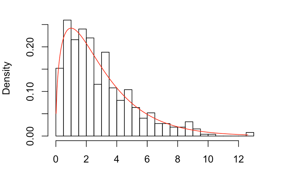
(a) $T_{\mathrm{out}}$

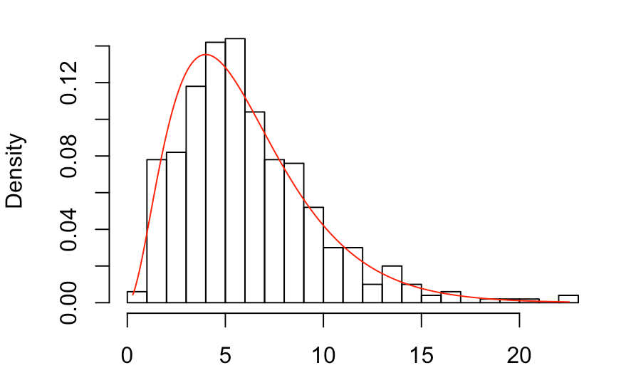
(b) $T_{\mathrm{both}}$

Figure 5: Empirical histograms for the test statistics $T_{\mathrm{out}}$ and $T_{\mathrm{both}}$ under the null hypothesis when $\rho=1.0$. The setting is that of directed mixed-membership graphs on $n=4800$ vertices. The red curve on the left panel is the probability density function for the $\chi^{2}_{3}$ distribution and the one on the right panel is the probability density function for the $\chi^{2}_{6}$ distribution.

References

- [1] {barticle}[author] \bauthor\bsnmAbbe, \bfnmE.\binitsE. (\byear2017). \btitleCommunity detection and stochastic block models: recent developments. \bjournalJournal of Machine Learning Research \bvolume18 \bpages6446–6531. \endbibitem
- [2] {binproceedings}[author] \bauthor\bsnmAdamic, \bfnmL. A.\binitsL. A. and \bauthor\bsnmGlance, \bfnmN.\binitsN. (\byear2005). \btitleThe political blogosphere and the 2004 US election: divided they blog. In \bbooktitleProceedings of the 3rd international workshop on Link discovery \bpages36–43. \endbibitem
- [3] {barticle}[author] \bauthor\bsnmAgterberg, \bfnmJ.\binitsJ., \bauthor\bsnmPark, \bfnmY.\binitsY., \bauthor\bsnmLarson, \bfnmJ.\binitsJ., \bauthor\bsnmWhite, \bfnmC.\binitsC., \bauthor\bsnmPriebe, \bfnmC. E.\binitsC. E. and \bauthor\bsnmLyzinski, \bfnmV.\binitsV. (\byear2020). \btitleVertex Nomination, consistent estimation, and adversarial modification. \bjournalElectronic Journal of Statistics \bpages3230–3267. \endbibitem
- [4] {barticle}[author] \bauthor\bsnmAiroldi, \bfnmE. M.\binitsE. M., \bauthor\bsnmBlei, \bfnmD. M.\binitsD. M., \bauthor\bsnmFienberg, \bfnmS. E.\binitsS. E. and \bauthor\bsnmXing, \bfnmE. P.\binitsE. P. (\byear2008). \btitleMixed membership stochastic blockmodels. \bjournalJournal of Machine Learning Research \bvolume9 \bpages1981–2014. \endbibitem
- [5] {barticle}[author] \bauthor\bsnmAthreya, \bfnmA.\binitsA., \bauthor\bsnmPriebe, \bfnmC. E.\binitsC. E., \bauthor\bsnmTang, \bfnmM.\binitsM., \bauthor\bsnmLyzinski, \bfnmV.\binitsV., \bauthor\bsnmMarchette, \bfnmD. J.\binitsD. J. and \bauthor\bsnmSussman, \bfnmD. L.\binitsD. L. (\byear2016). \btitleA limit theorem for scaled eigenvectors of random dot product graphs. \bjournalSankhya A \bvolume78 \bpages1–18. \endbibitem
- [6] {barticle}[author] \bauthor\bsnmBandeira, \bfnmA. S.\binitsA. S. and \bauthor\bsnmHandel, \bfnmR. Van\binitsR. V. (\byear2016). \btitleSharp nonasymptotic bounds on the norm of random matrices with independent entries. \bjournalAnnals of Probability \bvolume44 \bpages2479–2506. \endbibitem
- [7] {barticle}[author] \bauthor\bsnmBelkin, \bfnmM.\binitsM. and \bauthor\bsnmNiyogi, \bfnmP.\binitsP. (\byear2003). \btitleLaplacian eigenmaps for dimensionality reduction and data representation. \bjournalNeural Computation \bvolume15 \bpages1373-1396. \endbibitem
- [8] {barticle}[author] \bauthor\bsnmBhatia, \bfnmR.\binitsR. (\byear1987). \btitleSome Inequalities for Norm Ideals. \bjournalCommunications in Mathematical Physics \bvolume111 \bpages33–39. \endbibitem
- [9] {bbook}[author] \bauthor\bsnmBhatia, \bfnmR.\binitsR. (\byear1997). \btitleMatrix Analysis. \bpublisherSpringer. \endbibitem
- [10] {barticle}[author] \bauthor\bsnmBickel, \bfnmP. J.\binitsP. J. and \bauthor\bsnmSarkar, \bfnmP.\binitsP. (\byear2016). \btitleHypothesis testing for automated community detection in networks. \bjournalJournal of the Royal Statistical Society: Series B \bpages253–273. \endbibitem
- [11] {barticle}[author] \bauthor\bsnmCai, \bfnmT.\binitsT. and \bauthor\bsnmLi, \bfnmX.\binitsX. (\byear2015). \btitleRobust and computationally feasible community detection in the presence of arbitrary outlier nodes. \bjournalAnnals of Statistics \bvolume45 \bpages1027–1059. \endbibitem
- [12] {binproceedings}[author] \bauthor\bsnmChaudhuri, \bfnmK.\binitsK., \bauthor\bsnmChung, \bfnmF.\binitsF. and \bauthor\bsnmTsiatas, \bfnmA.\binitsA. (\byear2012). \btitleSpectral partitioning of graphs with general degrees and the extended planted partition model. In \bbooktitleProceedings of the 25th conference on learning theory. \endbibitem
- [13] {barticle}[author] \bauthor\bsnmChen, \bfnmK.\binitsK. and \bauthor\bsnmLei, \bfnmJ.\binitsJ. (\byear2018). \btitleNetwork cross-validation for determining the number of communities in network data. \bjournalJournal of the American Statistical Association \bvolume113 \bpages241–251. \endbibitem
- [14] {barticle}[author] \bauthor\bsnmCoifman, \bfnmR.\binitsR. and \bauthor\bsnmLafon, \bfnmS.\binitsS. (\byear2006). \btitleDiffusion maps. \bjournalApplied and Computational Harmonic Analysis \bvolume21 \bpages5–30. \endbibitem
- [15] {barticle}[author] \bauthor\bsnmDavis, \bfnmC.\binitsC. and \bauthor\bsnmKahan, \bfnmW.\binitsW. (\byear1970). \btitleThe rotation of eigenvectors by a pertubation. III. \bjournalSiam Journal on Numerical Analysis \bvolume7 \bpages1–46. \endbibitem
- [16] {barticle}[author] \bauthor\bsnmFan, \bfnmJ.\binitsJ., \bauthor\bsnmFan, \bfnmY.\binitsY., \bauthor\bsnmHan, \bfnmX.\binitsX. and \bauthor\bsnmLv, \bfnmJ.\binitsJ. (\byear2021+). \btitleAsymptotic Theory of Eigenvectors for Random Matrices with Diverging Spikes. \bjournalJournal of the American Statistical Association. \endbibitem
- [17] {barticle}[author] \bauthor\bsnmFan, \bfnmJ.\binitsJ., \bauthor\bsnmFan, \bfnmY.\binitsY., \bauthor\bsnmHan, \bfnmX.\binitsX. and \bauthor\bsnmLv, \bfnmJ.\binitsJ. (\byear2022+). \btitleSIMPLE: Statistical Inference on Membership Profiles in Large Networks. \bjournalJournal of the Royal Statistical Society, Series B. \endbibitem
- [18] {barticle}[author] \bauthor\bsnmFishkind, \bfnmD. E.\binitsD. E., \bauthor\bsnmLyzinski, \bfnmV.\binitsV., \bauthor\bsnmPao, \bfnmH.\binitsH., \bauthor\bsnmChen, \bfnmL.\binitsL. and \bauthor\bsnmPriebe, \bfnmC. E.\binitsC. E. (\byear2015). \btitleVertex nomination schemes for membership prediction. \bjournalAnnals of Applied Statistics \bvolume9 \bpages1510–1532. \endbibitem
- [19] {barticle}[author] \bauthor\bsnmGao, \bfnmC.\binitsC., \bauthor\bsnmMa, \bfnmZ.\binitsZ., \bauthor\bsnmZhang, \bfnmA. Y.\binitsA. Y. and \bauthor\bsnmZhou, \bfnmH. H.\binitsH. H. (\byear2017). \btitleAchieving optimal mis-classification proportion in stochastic blockmodels. \bjournalJournal of Machine Learning Research \bvolume18 \bpages1–45. \endbibitem
- [20] {barticle}[author] \bauthor\bsnmGhoshdastidar, \bfnmD.\binitsD., \bauthor\bsnmGutzeit, \bfnmM.\binitsM., \bauthor\bsnmCarpentier, \bfnmA.\binitsA. and \bauthor\bparticlevon \bsnmLuxburg, \bfnmU.\binitsU. (\byear2020). \btitleTwo-sample hypothesis testing for inhomogeneous random graphs. \bjournalAnnals of Statistics \bvolume48 \bpages2208–2229. \endbibitem
- [21] {binproceedings}[author] \bauthor\bsnmGilpin, \bfnmS.\binitsS., \bauthor\bsnmEliassi-Rad, \bfnmT.\binitsT. and \bauthor\bsnmDavidson, \bfnmI.\binitsI. (\byear2013). \btitleGuided learning for role discovery (GLRD): Framework, Algorithms, and Applications. In \bbooktitleProceedings of the 19th ACM SIGKDD Conference on Knowledge Discovery and Data Mining. \endbibitem
- [22] {barticle}[author] \bauthor\bsnmGinestet, \bfnmC. E.\binitsC. E., \bauthor\bsnmLi, \bfnmJ.\binitsJ., \bauthor\bsnmBalachandran, \bfnmP.\binitsP., \bauthor\bsnmRosenberg, \bfnmS.\binitsS. and \bauthor\bsnmKolaczyk, \bfnmE. D.\binitsE. D. (\byear2017). \btitleHypothesis testing for network data in functional neuroimaging. \bjournalAnnals of Applied Statistics \bvolume11 \bpages725–750. \endbibitem
- [23] {barticle}[author] \bauthor\bsnmGirvan, \bfnmM.\binitsM. and \bauthor\bsnmNewman, \bfnmM. EJ.\binitsM. E. (\byear2002). \btitleCommunity structure in social and biological networks. \bjournalProceedings of the national academy of sciences \bvolume99 \bpages7821–7826. \endbibitem
- [24] {barticle}[author] \bauthor\bsnmHoff, \bfnmP. D.\binitsP. D., \bauthor\bsnmRaftery, \bfnmA. E.\binitsA. E. and \bauthor\bsnmHandcock, \bfnmM. S.\binitsM. S. (\byear2002). \btitleLatent space approaches to social network analysis. \bjournalJournal of the American Statistical Association \bvolume97 \bpages1090–1098. \endbibitem
- [25] {barticle}[author] \bauthor\bsnmHolland, \bfnmP. W.\binitsP. W., \bauthor\bsnmLaskey, \bfnmK. B.\binitsK. B. and \bauthor\bsnmLeinhardt, \bfnmS.\binitsS. (\byear1983). \btitleStochastic blockmodels: First steps. \bjournalSocial networks \bvolume5 \bpages109–137. \endbibitem
- [26] {barticle}[author] \bauthor\bsnmHu, \bfnmJ.\binitsJ., \bauthor\bsnmQin, \bfnmH.\binitsH., \bauthor\bsnmYan, \bfnmT.\binitsT. and \bauthor\bsnmZhao, \bfnmY.\binitsY. (\byear2020). \btitleCorrected Bayesian information criterion for stochastic block models. \bjournalJournal of the American Statistical Association \bvolume115 \bpages1771–1783. \endbibitem
- [27] {barticle}[author] \bauthor\bsnmJin, \bfnmJiashun\binitsJ. (\byear2015). \btitleFast community detection by SCORE. \bjournalAnnals of Statistics \bvolume43 \bpages57–89. \endbibitem
- [28] {barticle}[author] \bauthor\bsnmKarrer, \bfnmB.\binitsB. and \bauthor\bsnmNewman, \bfnmM. EJ.\binitsM. E. (\byear2011). \btitleStochastic blockmodels and community structure in networks. \bjournalPhysical review E \bvolume83 \bpages016107. \endbibitem
- [29] {barticle}[author] \bauthor\bsnmKoo, \bfnmJohn\binitsJ., \bauthor\bsnmTang, \bfnmMinh\binitsM. and \bauthor\bsnmTrosset, \bfnmMichael W\binitsM. W. (\byear2021). \btitlePopularity Adjusted Block Models are Generalized Random Dot Product Graphs. \bjournalarXiv preprint arXiv:2109.04010. \endbibitem
- [30] {barticle}[author] \bauthor\bsnmLe, \bfnmC. M.\binitsC. M. and \bauthor\bsnmLevina, \bfnmE.\binitsE. (\byear2015). \btitleEstimating the number of communities in networks by spectral methods. \bjournalarXiv preprint arXiv:1507.00827. \endbibitem
- [31] {barticle}[author] \bauthor\bsnmLei, \bfnmJ.\binitsJ. (\byear2016). \btitleA goodness-of-fit test for stochastic block models. \bjournalAnnals of Statistics \bvolume44 \bpages401–424. \endbibitem
- [32] {barticle}[author] \bauthor\bsnmLei, \bfnmJ.\binitsJ. (\byear2021). \btitleNetwork representation using graph root distributions. \bjournalAnnals of Statistics \bvolume49 \bpages745–768. \endbibitem
- [33] {barticle}[author] \bauthor\bsnmLei, \bfnmJ.\binitsJ. and \bauthor\bsnmRinaldo, \bfnmA.\binitsA. (\byear2015). \btitleConsistency of spectral clustering in stochastic block models. \bjournalAnnals of Statistics \bvolume43 \bpages215–237. \endbibitem
- [34] {barticle}[author] \bauthor\bsnmLi, \bfnmT.\binitsT., \bauthor\bsnmLevina, \bfnmE.\binitsE. and \bauthor\bsnmZhu, \bfnmJ.\binitsJ. (\byear2020). \btitleNetwork cross-validation by edge sampling. \bjournalBiometrika \bvolume107 \bpages257–276. \endbibitem
- [35] {barticle}[author] \bauthor\bsnmMa, \bfnmS.\binitsS., \bauthor\bsnmSu, \bfnmL.\binitsL. and \bauthor\bsnmZhang, \bfnmY.\binitsY. (\byear2021). \btitleDetermining the Number of Communities in Degree-corrected Stochastic Block Models. \bjournalJournal of Machine Learning Research \bvolume22 \bpages1–63. \endbibitem
- [36] {bbook}[author] \bauthor\bsnmMarshall, \bfnmA. W.\binitsA. W., \bauthor\bsnmOlkin, \bfnmI.\binitsI. and \bauthor\bsnmArnold, \bfnmB. C.\binitsB. C. (\byear2011). \btitleInequalities: Theory of Majorization and its Applications, \bedition2nd ed. \bpublisherSpringer. \endbibitem
- [37] {barticle}[author] \bauthor\bsnmMcNemar, \bfnmQ.\binitsQ. (\byear1947). \btitleNote on the sampling error of the difference between correlated proportions or percentages. \bjournalPsychometrika \bvolume12 \bpages153–157. \endbibitem
- [38] {binproceedings}[author] \bauthor\bsnmNg, \bfnmA.\binitsA., \bauthor\bsnmJordan, \bfnmM.\binitsM. and \bauthor\bsnmWeiss, \bfnmY.\binitsY. (\byear2001). \btitleOn spectral clustering: analysis and an algorithm. In \bbooktitleAdvances in Neural Information Processing Systems \bvolume14. \endbibitem
- [39] {bphdthesis}[author] \bauthor\bsnmNickel, \bfnmC. L. M.\binitsC. L. M. (\byear2008). \btitleRandom dot product graphs a model for social networks, \btypePhD thesis, \bpublisherJohns Hopkins University. \endbibitem
- [40] {barticle}[author] \bauthor\bsnmNoroozi, \bfnmM.\binitsM., \bauthor\bsnmRimal, \bfnmR.\binitsR. and \bauthor\bsnmPensky, \bfnmM.\binitsM. (\byear2021). \btitleEstimation and clustering in popularity adjusted block model. \bjournalJournal of the Royal Statistical Society, Series B. \bvolume83 \bpages293–317. \endbibitem
- [41] {barticle}[author] \bauthor\bsnmOliveira, \bfnmR. I.\binitsR. I. (\byear2009). \btitleConcentration of the adjacency matrix and of the Laplacian in random graphs with independent edges. \bjournalarXiv preprint arXiv:0911.0600. \endbibitem
- [42] {barticle}[author] \bauthor\bsnmOstrowski, \bfnmA. M.\binitsA. M. (\byear1963). \btitleOn positive matrices. \bjournalMathematische Annalen \bvolume150 \bpages276–284. \endbibitem
- [43] {barticle}[author] \bauthor\bsnmRohe, \bfnmK.\binitsK., \bauthor\bsnmChatterjee, \bfnmS.\binitsS. and \bauthor\bsnmYu, \bfnmB.\binitsB. (\byear2011). \btitleSpectral clustering and the high-dimensional stochastic blockmodel. \bjournalAnnals of Statistics \bvolume39 \bpages1878–1915. \endbibitem
- [44] {barticle}[author] \bauthor\bsnmRubin-Delanchy, \bfnmP.\binitsP., \bauthor\bsnmCape, \bfnmJ.\binitsJ., \bauthor\bsnmTang, \bfnmM.\binitsM. and \bauthor\bsnmPriebe, \bfnmC. E.\binitsC. E. (\byear2022+). \btitleA statistical interpretation of spectral embedding: the generalised random dot product graph. \bjournalJournal of the Royal Statistical Society, Series B. \endbibitem
- [45] {barticle}[author] \bauthor\bsnmSengupta, \bfnmSrijan\binitsS. and \bauthor\bsnmChen, \bfnmYuguo\binitsY. (\byear2018). \btitleA block model for node popularity in networks with community structure. \bjournalJournal of the Royal Statistical Society: Series B (Statistical Methodology) \bvolume80 \bpages365–386. \endbibitem
- [46] {bbook}[author] \bauthor\bsnmSerre, \bfnmD.\binitsD. (\byear2002). \btitleMatrices: Theory and Applications. \bpublisherSpringer. \endbibitem
- [47] {barticle}[author] \bauthor\bsnmStewart, \bfnmG. W.\binitsG. W. (\byear1977). \btitleOn the perturbation of pseudo-inverses, projections, and linear least squares problems. \bjournalSIAM Review \bvolume19 \bpages634–662. \endbibitem
- [48] {barticle}[author] \bauthor\bsnmSussman, \bfnmD. L.\binitsD. L., \bauthor\bsnmTang, \bfnmM.\binitsM., \bauthor\bsnmFishkind, \bfnmD. E.\binitsD. E. and \bauthor\bsnmPriebe, \bfnmC. E.\binitsC. E. (\byear2012). \btitleA consistent adjacency spectral embedding for stochastic blockmodel graphs. \bjournalJournal of the American Statistical Association \bvolume107 \bpages1119–1128. \endbibitem
- [49] {barticle}[author] \bauthor\bsnmTang, \bfnmM.\binitsM., \bauthor\bsnmAthreya, \bfnmA.\binitsA., \bauthor\bsnmSussman, \bfnmD. L.\binitsD. L., \bauthor\bsnmLyzinski, \bfnmV.\binitsV., \bauthor\bsnmPark, \bfnmY.\binitsY. and \bauthor\bsnmPriebe, \bfnmC. E.\binitsC. E. (\byear2017). \btitleA semiparametric two-sample hypothesis testing problem for random graphs. \bjournalJournal of Computational and Graphical Statistics \bvolume26 \bpages344–354. \endbibitem
- [50] {barticle}[author] \bauthor\bsnmTang, \bfnmM.\binitsM. and \bauthor\bsnmPriebe, \bfnmC. E.\binitsC. E. (\byear2018). \btitleLimit theorems for eigenvectors of the normalized Laplacian for random graphs. \bjournalAnnals of Statistics \bvolume46 \bpages2360–2415. \endbibitem
- [51] {barticle}[author] \bauthor\bparticlevon \bsnmLuxburg, \bfnmU.\binitsU., \bauthor\bsnmBelkin, \bfnmM.\binitsM. and \bauthor\bsnmBousquet, \bfnmO.\binitsO. (\byear2008). \btitleConsistency of spectral clustering. \bjournalAnnals of Statistics \bvolume36 \bpages555–586. \endbibitem
- [52] {barticle}[author] \bauthor\bsnmWang, \bfnmBo\binitsB., \bauthor\bsnmPourshafeie, \bfnmArmin\binitsA., \bauthor\bsnmZitnik, \bfnmMarinka\binitsM., \bauthor\bsnmZhu, \bfnmJunjie\binitsJ., \bauthor\bsnmBustamante, \bfnmCarlos D\binitsC. D., \bauthor\bsnmBatzoglou, \bfnmSerafim\binitsS. and \bauthor\bsnmLeskovec, \bfnmJure\binitsJ. (\byear2018). \btitleNetwork enhancement as a general method to denoise weighted biological networks. \bjournalNature communications \bvolume9 \bpages1–8. \endbibitem
- [53] {barticle}[author] \bauthor\bsnmWang, \bfnmYX. R.\binitsY. R. and \bauthor\bsnmBickel, \bfnmP. J.\binitsP. J. (\byear2017). \btitleLikelihood-based model selection for stochastic block models. \bjournalAnnals of Statistics \bvolume45 \bpages500–528. \endbibitem
- [54] {barticle}[author] \bauthor\bsnmYan, \bfnmX.\binitsX., \bauthor\bsnmShalizi, \bfnmC.\binitsC., \bauthor\bsnmJensen, \bfnmJ. E.\binitsJ. E., \bauthor\bsnmKrzakala, \bfnmF.\binitsF., \bauthor\bsnmMoore, \bfnmC.\binitsC., \bauthor\bsnmZdeborová, \bfnmL.\binitsL., \bauthor\bsnmZhang, \bfnmP.\binitsP. and \bauthor\bsnmZhu, \bfnmY.\binitsY. (\byear2014). \btitleModel selection for degree-corrected block models. \bjournalJournal of Statistical Mechanics: Theory and Experiment \bvolume2014 \bpagesP05007. \endbibitem