A dynamically-consistent nonstandard finite difference scheme for the SICA model

Abstract

In this work, we derive a nonstandard finite difference scheme for the SICA (Susceptible–Infected–Chronic–AIDS) model and analyze the dynamical properties of the discretized system. We prove that the discretized model is dynamically consistent with the continuous, maintaining the essential properties of the standard SICA model, namely, the positivity and boundedness of the solutions, equilibrium points, and their local and global stability.

1 Introduction

The Human Immunodeficiency Virus (HIV) is responsible for a very high number of deaths worldwide. Acquired ImmunoDeficiency Syndrome (AIDS) is a disease of the human immune system caused by infection with HIV. The HIV virus can be transmitted by several ways but there is no cure or vaccine for AIDS. Nevertheless, antiretroviral (ART) treatment improves health, prolongs life and reduces the risk of HIV transmission. The ART treatment increases life expectation but has some limitations. For instance, it doesn’t restore health, has some side effects, and is very expensive. Individuals infected with HIV are more likely to develop tuberculosis because of their immunodeficiency, so a model that considers HIV and tuberculosis is very interesting to investigate. One can find many studies in the literature [1, 2, 3]. A TB-HIV/AIDS co-infection model, that contains the celebrated SICA (Susceptible–Infected–Chronic–AIDS) model as a sub-model, was first proposed in [4]:

$$\begin{cases}\dot{S}(t)=\Lambda-\lambda(t)S(t)-\mu S(t),\\[5.69046pt] \dot{I}(t)=\lambda(t)S(t)-(\rho+\phi+\mu)I(t)+\alpha A(t)+\omega C(t),\\[5.69046pt] \dot{C}(t)=\phi I(t)-(\omega+\mu)C(t),\\[5.69046pt] \dot{A}(t)=\rho\,I(t)-(\alpha+\mu+d)A(t),\end{cases}$$ (1.1)

where

$$\lambda(t)=\frac{\beta}{N(t)}\left[I(t)+\eta_{C}C(t)+\eta_{A}A(t)\right]$$ (1.2)

with

$$N(t)=S(t)+I(t)+C(t)+A(t)$$ (1.3)

the total population at time $t$. The meaning of the parameters that appear in the SICA model (1.1)–(1.3) are given in Table 1.

Table 1: Parameters of the SICA model (1.1)–(1.3).

Symbol	Description
$N(0)$	Initial population
$\Lambda$	Recruitment rate
$\mu$	Natural death rate
$\beta$	HIV transmission rate
$\phi$	HIV treatment rate for $I$ individuals
$\rho$	Default treatment rate for $I$ individuals
$\alpha$	AIDS treatment rate
$\omega$	Default treatment rate for $C$ individuals
$d$	AIDS induced death rate
$\eta_{C}$	Modification parameter
$\eta_{A}$	Modification parameter

The model considers a varying population size in a homogeneously mixing population, subdividing the human population into four mutually-exclusive compartments:

• susceptible individuals ($S$);

• HIV-infected individuals with no clinical symptoms of AIDS (the virus is living or developing in the individuals but without producing symptoms or only mild ones) but able to transmit HIV to other individuals ($I$);

• HIV-infected individuals under ART treatment (the so called chronic stage) with a viral load remaining low ($C$);

• HIV-infected individuals with AIDS clinical symptoms ($A$).

The SICA model has some assumptions. It can be seen in [5] that the susceptible population is increased by the recruitment of individuals into the population, assumed susceptible at a rate $\Lambda$. All individuals suffer from natural death at a constant rate $\mu$. Susceptible individuals $S$ acquire HIV infection, following effective contact with people infected with HIV, at rate $\lambda$ (1.2), where $\beta$ is the effective contact rate for HIV transmission. The modification parameter $\eta_{A}\geq 1$ accounts for the relative infectiousness of individuals with AIDS symptoms, in comparison to those infected with HIV with no AIDS symptoms. Individuals with AIDS symptoms are more infectious than HIV-infected individuals because they have a higher viral load and there is a positive correlation between viral load and infectiousness. On the other hand, $\eta_{C}\leq 1$ translates the partial restoration of the immune function of individuals with HIV infection that use correctly ART. The SICA mathematical model (1.1)–(1.3) is well-studied in the literature [5]. It has shown to provide a proper description with respect to the HIV/AIDS situation in Cape Verde [6] and recent extensions include stochastic transmission [7] and fractional versions with memory and general incidence rates [8]. Here our main aim is to propose, for the first time in the literature, a discrete-time SICA model.

For most nonlinear continuous models in engineering and natural sciences, it is not possible to obtain an exact solution [9], so a variety of methods have been constructed to compute numerical solutions [10, 11]. It is well known that numerical methods, like the Euler and Runge–Kutta, among others, often fail to solve nonlinear systems. One of the reasons is that they generate oscillations and unsteady states if the time step size decreases to a critical size [12]. Among available approaches to address the problem, the nonstandard finite discrete difference (NSFD) schemes, introduced by Mickens in [13, 14], have been successfully applied to several different epidemiological models [15, 16]. Precisely, the NSFD schemes were created to eliminate or reduce the occurrence of numerical instabilities that generally arise while using other methods. This is possible because there are some designed laws that systems must satisfy in order to preserve the qualitative properties of the continuous model, such as positivity, boundedness, stability of the equilibrium points, conservation laws, and others [17]. The literature on Mickens-type NSFD schemes is now vast [18, 19]. The paper [20] considers the NSFD method of Mickens and apply it to a dynamical system that models the Ebola virus disease. In [21], a NSFD scheme is designed in which the Metzler matrix structure of the continuous model is carefully incorporated and both Mickens’ rules on the denominator of the discrete derivative and the nonlocal approximation of nonlinear terms are used. In that work the general analysis is detailed for a MSEIR model. In [22], the authors summarize NSFD methods and compare their performance for various step-sizes when applied to a specific two-sex (male/female) epidemic model; while in [23] it is shown that Mickens’ approach is qualitatively superior to the standard approach in constructing numerical methods with respect to productive-destructive systems (PDS’s). NSFD schemes for PDS’s are also investigated in [24]; NSFD methods for predator-prey models with the Beddington–De Angelis functional response are studied in [25]. Here we propose and investigate, for the first time in the literature, the dynamics of a discretized SICA model using the Mickens NSFD scheme.

The paper is organized as follows. Some considerations, regarding the continuous SICA model and the stability of discrete-time systems, are presented in section 2. The original results are then given in section 3: we start by introducing the discretized SICA model; we find the equilibrium points, prove the positivity, Theorem 3, and boundedness of the solutions, Theorem 4; we also establish the local stability of the disease free equilibrium point of the discrete model, Theorem 5, as well as the global stability of the equilibrium points, Theorems 6 and 7. In section 4, we provide some numerical simulations to illustrate the stability of the NSFD discrete SICA model using a case study. We end with section 5 of conclusion.

2 Preliminaries

In this section, we collect some preliminary results about the continuous SICA model [4], as well as results for the stability of discrete-time systems [26], useful in our work.

2.1 The continuous SICA model

All the information in this section is proved in [4]. Each solution $(S(t),I(t),C(t),A(t))$ of the continuous model much satisfy $S(0)\geq 0$, $I(0)\geq 0$, $C(0)\geq 0$, and $A(0)\geq 0$, because each equation represents groups of human beings. Adding the four equations of (1.1), one has

$$\dfrac{dN}{dt}=\Lambda-\mu N-dA\leq\Lambda-\mu N,$$

so that

$$N(t)\leq\dfrac{\Lambda}{\mu}+\left(N_{0}-\dfrac{\Lambda}{\mu}\right)\operatorname{e}^{-\mu t}.$$

Therefore, the biologically feasible region is given by

$$\Omega=\left\{(S,I,C,A)\in(\operatorname{\mathbbm{R}}_{0}^{4})^{+}:0\leq S+I+C+A\leq\frac{\Lambda}{\mu}\right\},$$ (2.1)

which is positively invariant and compact. This means that it is sufficient to study the qualitative dynamics in $\Omega$. The model has two equilibrium points: a disease free and an endemic one. The disease free equilibrium (DFE) point is given by

$$(S^{\ast},I^{\ast},C^{\ast},A^{\ast})=\left(\frac{\Lambda}{\mu},0,0,0\right).$$

Following the approach of the next generation matrix [27], the basic reproduction number $R_{0}$ for model (1.1), which represents the expected average number of new infections produced by a single HIV-infected individual in contact with a completely susceptible population, is given by

$$R_{0}=\dfrac{\beta(C_{3}C_{2}+\rho\eta_{A}C_{3}+\phi\eta_{C}C_{2})}{\rho C_{3}(\mu+d)+\mu C_{2}(C_{3}+\phi)}=:\dfrac{\mathcal{N}}{\mathcal{D}},$$

where along all the manuscript we use $C_{1}=\rho+\phi+\mu$, $C_{2}=\alpha+\mu+d$, and $C_{3}=\omega+\mu$. The endemic point has the following expression:

$$(S^{\ast},I^{\ast},C^{\ast},A^{\ast})=\left(\frac{\Lambda}{\lambda^{\ast}+\mu},-\frac{\lambda^{\ast}\Lambda C_{2}C_{3}}{D},-\frac{\phi\lambda^{\ast}\Lambda C_{2}}{D},-\frac{\rho\lambda^{\ast}\Lambda C_{3}}{D}\right),$$

where $D=-(\lambda^{\ast}+\mu)(\mu(C_{3}(\rho+C_{2})+C_{2}\phi+\rho d)+\rho\omega d)$ and

$$\lambda^{\ast}=\dfrac{\beta(I^{\ast}+\eta_{C}C^{\ast}+\eta_{A}A^{\ast})}{N^{\ast}}=\dfrac{\mathcal{D}(\mathcal{R}_{0}-1)}{C_{2}C_{3}+\phi C_{2}+\rho C_{3}},$$ (2.2)

which is positive if $\mathcal{R}_{0}>1$. The explicit expression of the endemic equilibrium point of (1.1) is given by

$$S^{\ast}=\dfrac{\Lambda(\mathcal{D}-\rho dC_{3})}{\mu(\mathcal{N}-\rho dC_{3})},\quad I^{\ast}=\dfrac{\Lambda C_{2}C_{3}(\mathcal{D}-\mathcal{N})}{\mathcal{D}(\rho dC_{3}-\mathcal{N})},\quad C^{\ast}=\dfrac{\Lambda C_{2}\phi(\mathcal{D}-\mathcal{N})}{\mathcal{D}(\rho dC_{3}-\mathcal{N})},\quad A^{\ast}=\dfrac{\Lambda\rho C_{3}(\mathcal{D}-\mathcal{N})}{\mathcal{D}(\rho dC_{3}-\mathcal{N})}.$$

Regarding the stability of the equilibrium points, Theorem 3.1 and Proposition 3.4 of [4] establish the persistence of the endemic point. The disease is persistent in the population if the infected cases with AIDS are bounded away from zero or the population $S$ disappears. The local stability of the endemic point is given in Theorem 3.8 of [4]. Lemma 3.5 of [4] states that the DFE is locally asymptotically stable if $R_{0}<1$ and unstable if $R_{0}>1$. Finally, Theorem 3.6 of [4] asserts that, under suitable conditions, the DFE point is globally asymptotically stable. Here we prove similar properties in the discrete-time setting (section 3). For that we now recall an important tool for difference equations.

2.2 The Schur–Cohn criterion

One of the main tools that provides necessary and sufficient conditions for the zeros of a $n$th-degree polynomial

$$p(\lambda)=\lambda^{k}+p_{1}\lambda^{k-1}+\cdots+p_{k}$$ (2.3)

to lie inside the unit disk is the Schur–Cohn criterion [26]. This result is useful for studying the stability of the zero solution of a $k$th-order difference equation or to investigate the stability of a $k$-dimensional system of the form

$$x(n+1)=Ax(n),$$

where $p(\lambda)$ in (2.3) is the characteristic polynomial of the matrix $A$. Let us introduce some preliminaries before presenting the Schur–Cohn criterion. Namely, let us define the inners of a matrix $B=(b_{ij})$. The inners of a matrix are the matrix itself and all the matrices obtained by omitting successively the first and last columns and first and last rows. A matrix $B$ is said to be positive innerwise if the determinant of all its inners are positive.

Theorem 1 (The Shur–Cohn criterion [26]).

The zeros of the characteristic polynomial (2.3) lie inside the unit disk if, and only if, the following holds:

1. $p(1)>0$;

2. $(-1)^{k}p(-1)>0$;

3. the $(k-1)\times(k-1)$ matrices

   $$B_{k-1}^{\pm}=\left(\begin{array}[]{ccccc}1&0&\cdots&&0\\ p_{1}&1&\cdots&&0\\ \vdots&&&&\vdots\\ p_{k-3}&&&&p_{1}\\ p_{k-2}&p_{k-3}&\cdots&p_{1}&1\\ \end{array}\right)\pm\left(\begin{array}[]{ccccc}0&0&\cdots&0&p_{k}\\ 0&0&\cdots&p_{k}&p_{k-1}\\ \vdots&\vdots&&&\vdots\\ 0&p_{k}&&&p_{3}\\ p_{k}&p_{k-1}&\cdots&p_{3}&p_{2}\\ \end{array}\right)$$

   are positive innerwise.

Using the Schur–Cohn criterion, one may obtain necessary and sufficient conditions on the $p_{i}$ coefficients such that the zero solution of (2.3) is locally asymptotically stable.

Theorem 2 (See [26]).

Let $A\in\mathcal{M}_{k\times k}$ and let (2.3) be its characteristic polynomial. Then, $p(\lambda)$ is a polynomial of degree $k$. Moreover, $p(\lambda)$ has the form

$$p(\lambda)=(-1)^{k}\lambda^{k}+(-1)^{k-1}Tr(A)\lambda^{k-1}+\cdots+\det(A).$$ (2.4)

3 Main results

We begin by proposing a discrete-time SICA model.

3.1 The NSFD scheme

One of the important features of the discrete-time epidemic models obtained by Mickens method is that they present the same features as the corresponding original continuous-time models. Here, we construct a dynamically consistent numerical NSFD scheme for solving (1.1) based on [13, 14, 17]. Let us define the time instants $t_{n}=nh$ with $n$ integer, $h=t_{n+1}-t_{n}$ as the time step size, and $(S_{n},I_{n},C_{n},A_{n})$ as the approximated values of $(S(nh),I(nh),C(nh),A(nh))$. Thus, the NSFD scheme for model (1.1) takes the following form:

$$\begin{cases}\dfrac{S_{n+1}-S_{n}}{\psi(h)}=\Lambda-\tilde{\lambda}_{n}S_{n+1}-\mu S_{n+1},\\[5.69046pt] \dfrac{I_{n+1}-I_{n}}{\psi(h)}=\tilde{\lambda}_{n}S_{n+1}-(\rho+\phi+\mu)I_{n+1}+\alpha A_{n+1}+\omega C_{n+1},\\[5.69046pt] \dfrac{C_{n+1}-C_{n}}{\psi(h)}=\phi I_{n+1}-(\omega+\mu)C_{n+1},\\[5.69046pt] \dfrac{A_{n+1}-A_{n}}{\psi(h)}=\rho\,I_{n+1}-(\alpha+\mu+d)A_{n+1},\end{cases}$$ (3.1)

where $\tilde{\lambda}_{n}=\frac{\beta}{N_{n}}(I_{n}+\eta_{C}C_{n}+\eta_{A}A_{n})$. The nonstandard schemes are based in two fundamental principles [14, 17]:

1. Regarding the first derivative, we have

   $$\dfrac{dx}{dt}\rightarrow\dfrac{x_{k+1}-\nu(h)x_{k}}{\psi(h)},$$

   where $\nu(h)$ and $\psi(h)$ are the numerator and denominator functions that satisfy the requirements

   $$\nu(h)=1+O(h^{2}),\qquad\psi(h)=h+O(h^{2}).$$

   In general, the numerator function can be selected to be $\nu(h)=1$. We will make this choice here. Generally, the denominator function is nontrivial. Based on Mickens work [28, 29], when we write explicitly $S_{n+1}$ using $\phi(h)=h$, we have in the denominator the term $1+\mu h$, which means that we can use $\psi(h)=\dfrac{\operatorname{e}^{\mu h}-1}{\mu}$ as the denominator function. Throughout our study, $\psi(h)=\dfrac{\operatorname{e}^{\mu h}-1}{\mu}$ but, for brevity, we write $\psi(h)=\psi$.

2. Both linear and nonlinear functions of $x(t)$ and its derivatives may require a “nonlocal” discretization. For example, $x^{2}$ can be replaced by $x_{k}x_{k+1}$.

Since model (3.1) is linear in $S_{n+1}$, $I_{n+1}$, $C_{n+1}$, and $A_{n+1}$, we can obtain their explicit form:

$$\begin{cases}S_{n+1}=\dfrac{S_{n}+\Lambda\psi}{1+\mu\psi+\frac{\beta\psi}{N_{n}}\left(I_{n}+\eta_{C}C_{n}+\eta_{A}A_{n}\right)},\\[8.5359pt] I_{n+1}=\dfrac{\left(I_{n}+\frac{\beta\psi S_{n+1}(I_{n}+\eta_{C}C_{n}+\eta_{A}A_{n})}{N_{n}}\right)(1+C_{2}\psi)(1+C_{3}\psi)+\alpha\psi A_{n}(1+C_{3}\psi)+\omega\phi C_{n}(1+C_{2}\psi)}{(1+C_{1}\psi)(1+C_{2}\psi)(1+C_{3}\psi)-\alpha\rho\psi^{2}(1+C_{3}\psi)-\omega\phi\psi^{2}(1+C_{2}\psi)},\\[8.5359pt] C_{n+1}=\dfrac{\phi\psi I_{n+1}+C_{n}}{1+C_{3}\psi},\\[8.5359pt] A_{n+1}=\dfrac{\rho\psi I_{n+1}+A_{n}}{1+C_{2}\psi}.\end{cases}$$ (3.2)

3.2 Positivity of solutions

The first result to be shown is the positivity of the solutions.

Theorem 3.

If all the initial and parameter values of the discrete system (3.2) are positive, then the solutions are always positive for all $n\geq 0$ with denominator function $\psi$.

Proof.

Let us assume that $S(0),I(0),C(0),A(0)$ are positive. We only need to show that $I_{n+1}$ is positive. The denominator is given by

$$(1+C_{1}\psi)(1+C_{2}\psi)(1+C_{3}\psi)-\alpha\rho\psi^{2}(1+C_{3}\psi)-\omega\phi\psi^{2}(1+C_{2}\psi),$$ (3.3)

which can be rewritten as

$$1+(C_{1}+C_{2}+C_{3})\psi+(C_{1}C_{2}+C_{1}C_{3}+C_{2}C_{3}-\phi\omega-\alpha\rho)\psi^{2}+(C_{1}C_{2}C_{3}-C_{2}\phi\omega-\alpha\rho C_{3})\psi^{3}$$

and, simplifying, we get

$$1+(C_{1}+C_{2}+C_{3})\psi+\left(C_{2}(2\mu+\phi+\omega)+C_{3}(\omega+\rho)+\mu(\phi+\rho)+\rho d\right)\psi^{2}\\ +(C_{3}\rho(\mu+d)+C_{2}\mu(C_{3}+\phi))\psi^{3}.$$

Since all parameter values are positive, $(S_{n+1},I_{n+1},C_{n+1},A_{n+1})$ is positive for all $n\geq 0$. ∎

3.3 Conservation law

The second result to be shown is the conservation law or boundedness of the solutions.

Theorem 4.

The NSFD scheme defines the discrete dynamical system (3.2) on

$$\tilde{\Omega}=\left\{(S_{n},I_{n},C_{n},A_{n}):0\leq S_{n}+I_{n}+C_{n}+A_{n}\leq\frac{\Lambda}{\mu}\right\}.$$ (3.4)

Proof.

Let the total population be $N_{n}=S_{n}+I_{n}+C_{n}+A_{n}$. Adding the four equations of (3.1), we have

$$\dfrac{N_{n+1}-N_{n}}{\psi}=\Lambda-\mu N_{n+1}-dA_{n+1}\Leftrightarrow(1+\mu\psi)N_{n+1}=\Lambda\psi+N_{n}-d\psi A_{n+1}\\$$

and

$$N_{n+1}\leq\frac{\Lambda\psi}{1+\mu\psi}+\dfrac{N_{n}}{1+\mu\psi}\Leftrightarrow N_{n}\leq\Lambda\psi\sum_{j=1}^{n}\left(\frac{1}{1+\mu\psi}\right)^{j}+N_{0}\left(\frac{1}{1+\mu\psi}\right)^{n}.$$

By the discrete Grownwall inequality, if $0<N(0)<\frac{\Lambda}{\mu}$, then

$$N_{n}\leq\frac{\Lambda}{\mu}\left(1-\frac{1}{(1+\mu\psi)^{n}}\right)+N_{0}\left(\frac{1}{1+\mu\psi}\right)^{n}=\dfrac{\Lambda}{\mu}+\left(N_{0}-\frac{\Lambda}{\mu}\right)\left(\dfrac{1}{1+\mu\psi}\right)^{n}$$ (3.5)

and, since $\left(\dfrac{1}{1+\mu\psi}\right)<1$, we have $N_{n}\to\frac{\Lambda}{\mu}$ as $n\to\infty$. We conclude that the feasible region $\tilde{\Omega}$ is maintained within the discrete scheme. ∎

3.4 Elementary stability

A difference scheme that approximates a first-order differential system is elementary stable if, for any value of the step size, its fixed-points are exactly those of the differential system. Furthermore, when applied to the associated linearized differential system, the resulting difference scheme has the same stability/instability properties [30].

The continuous and discrete system have the same equilibria. The disease free equilibrium (DFE) point is given by

$$E_{0}=(S^{\ast},I^{\ast},C^{\ast},A^{\ast})=\left(\frac{\Lambda}{\mu},0,0,0\right).$$ (3.6)

The explicit expression of the endemic equilibrium point of (3.2) can be rewritten as the one of the continuous case: when

$$\lambda^{\ast}=\dfrac{\beta(I^{\ast}+\eta_{C}C^{\ast}+\eta_{A}A^{\ast})}{N^{\ast}}=\dfrac{\mathcal{D}(\mathcal{R}_{0}-1)}{C_{2}C_{3}+\phi C_{2}+\rho C_{3}},$$

we obtain the endemic equilibrium point. The explicit expression of the endemic equilibrium point of (3.2) can be rewritten as the one of the continuous case:

$$S^{\ast}=\dfrac{\Lambda(\mathcal{D}-\rho dC_{3})}{\mu(\mathcal{N}-\rho dC_{3})},\quad I^{\ast}=\dfrac{\Lambda C_{2}C_{3}(\mathcal{D}-\mathcal{N})}{\mathcal{D}(\rho dC_{3}-\mathcal{N})},\quad C^{\ast}=\dfrac{\Lambda C_{2}\phi(\mathcal{D}-\mathcal{N})}{\mathcal{D}(\rho dC_{3}-\mathcal{N})},\quad A^{\ast}=\dfrac{\Lambda\rho C_{3}(\mathcal{D}-\mathcal{N})}{\mathcal{D}(\rho dC_{3}-\mathcal{N})}.$$ (3.7)

After some computations, we get the following equalities:

$$\begin{split}S^{\ast}&=\dfrac{\Lambda}{\lambda^{\ast}+\mu}=\dfrac{\Lambda(C_{2}C_{3}+C_{2}\phi+\rho C_{3})}{\mathcal{D}(\mathcal{R}_{0}-1)+\mu(C_{2}C_{3}+C_{2}\phi+\rho C_{3})}=\dfrac{\Lambda(\mathcal{D}-\rho dC_{3})}{\mu(\mathcal{N}-\rho dC_{3})},\\ I^{\ast}&=\dfrac{S^{\ast}\lambda^{\ast}C_{2}C_{3}}{\mathcal{D}}=\dfrac{\Lambda(R_{0}-1)C_{2}C_{3}}{\mathcal{D}(\mathcal{R}_{0}-1)+\mu(C_{2}C_{3}+C_{2}\phi+\rho C_{3})}=\dfrac{\Lambda C_{2}C_{3}(\mathcal{D}-\mathcal{N})}{\mathcal{D}(\rho dC_{3}-\mathcal{N})},\\ C^{\ast}&=\dfrac{S^{\ast}\lambda^{\ast}\phi C_{2}}{\mathcal{D}}=\dfrac{\Lambda(R_{0}-1)C_{2}\phi}{\mathcal{D}(\mathcal{R}_{0}-1)+\mu(C_{2}C_{3}+C_{2}\phi+\rho C_{3})}=\dfrac{\Lambda C_{2}\phi(\mathcal{D}-\mathcal{N})}{\mathcal{D}(\rho dC_{3}-\mathcal{N})},\\ A^{\ast}&=\dfrac{S^{\ast}\lambda^{\ast}\rho C_{3}}{\mathcal{D}}=\dfrac{\Lambda(R_{0}-1)\rho C_{3}}{\mathcal{D}(\mathcal{R}_{0}-1)+\mu(C_{2}C_{3}+C_{2}\phi+\rho C_{3})}=\dfrac{\Lambda\rho C_{3}(\mathcal{D}-\mathcal{N})}{\mathcal{D}(\rho dC_{3}-\mathcal{N})}.\end{split}$$

3.4.1 Local stability of the DFE point

Let us discuss the stability of the proposed NSFD scheme at the DFE point $E_{0}$ (3.6).

Remark 1.

Several articles use the next-generation matrix approach presented in [31]. For that, however, the matrices $F+T$ must be non-negative. Our model does not satisfy such condition.

The following technical lemma has an important role in our proofs.

Lemma 1.

If $\mathcal{R}_{0}<1$, then $\beta$ must be smaller than $C_{1}$.

Proof.

If $\mathcal{R}_{0}<1$, then

$$\dfrac{\beta(C_{2}C_{3}+C_{3}\eta_{A}\rho+C_{2}\eta_{C}\phi)}{C_{1}C_{2}C_{3}-C_{3}\alpha\rho-C_{2}\omega\phi}<1 \Leftrightarrow\beta(C_{2}C_{3}+C_{3}\eta_{A}\rho+C_{2}\eta_{C}\phi)<C_{1}C_{2}C_{3}-C_{3}\alpha\rho-C_{2}\omega\phi$$

$$\Leftrightarrow\beta(C_{2}C_{3}+C_{3}\eta_{A}\rho+C_{2}\eta_{C}\phi)-C_{1}C_{2}C_{3}-C_{3}\alpha\rho-C_{2}\omega\phi<0$$

$$\Leftrightarrow(\beta-C_{1})C_{2}C_{3}<-\beta C_{3}\eta_{A}\rho-\beta C_{2}\eta_{C}\phi-C_{3}\alpha\rho-C_{2}\omega\phi<0.$$

Since $C_{2}$ and $C_{3}$ are positive, we conclude that $\beta-C_{1}<0$. ∎

Proposition 1.

The first condition of Theorem 1, $p_{4}(1)>0$, is satisfied if $\mathcal{R}_{0}<1$.

Proof.

The linearization of (3.2) at the DFE $E_{0}$ is:

$$J(E_{0})=\left(\begin{array}[]{cccc}-\mu&-\beta&-\beta\eta_{C}&-\beta\eta_{A}\\ 0&\beta-(\rho+\phi+\mu)&\beta\eta_{c}+\omega&\beta\eta_{A}+\alpha\\ 0&\phi&-(\omega+\mu)&0\\ 0&\rho&0&-(\alpha+\mu+d)\end{array}\right)=\left(\begin{array}[]{cccc}-\mu&-\beta&-\beta\eta_{C}&-\beta\eta_{A}\\ 0&\beta-C_{1}&\beta\eta_{c}+\omega&\beta\eta_{A}+\alpha\\ 0&\phi&-C_{3}&0\\ 0&\rho&0&-C_{2}\end{array}\right).$$

The characteristic polynomial of $J(E_{0})$ has the following expression:

$$p_{4}(\lambda)=\lambda^{4}+p_{1}\lambda^{3}+p_{2}\lambda^{2}+p_{3}\lambda+p_{4}=(-\mu-\lambda)p_{3}(\lambda),$$

where $p_{3}(\lambda)$ is given by

$$\begin{split}p_{3}(\lambda)&=-\lambda^{3}+(\beta-C_{1}-C_{2}-C_{3})\lambda^{2}+((\beta-C_{1})(C_{2}+C_{3})-C_{2}C_{3}+(\beta\eta_{A}+\alpha)\rho+(\beta\eta_{C}+\omega)\phi)\lambda\\ &\quad+(-C_{1}C_{2}C_{3}+C_{2}C_{3}\beta+C_{3}\alpha\rho+C_{3}\beta\eta_{A}\rho+C_{2}\beta\eta_{C}\phi+C_{2}\phi\omega),\end{split}$$

that is,

$$\begin{split}p_{3}(\lambda)&=-\lambda^{3}+(\beta-C_{1}-C_{2}-C_{3})\lambda^{2}+\left((\beta-C_{1})(C_{2}+C_{3})-C_{2}C_{3}+(\beta\eta_{A}+\alpha)\rho+(\beta\eta_{C}+\omega)\phi\right)\lambda\\ &\quad+(\mathcal{N}-\mathcal{D}).\end{split}$$

Since $p_{4}(1)>0$, we have $(-\mu-1)p_{3}(1)>0$, and recalling that $\mu>0$, we conclude that

$$p_{3}(1)=-1+(\beta-C_{1}-C_{2}-C_{3})+(\beta-C_{1})(C_{2}+C_{3})-C_{2}C_{3}+\rho(\beta\eta_{A}+\alpha)+\phi(\beta\eta_{C}+\omega)-\mathcal{D}(1-\mathcal{R}_{0})$$

is negative: $p_{3}(1)<0$. If $\mathcal{R}_{0}<1$, then

$$0<\rho(\beta\eta_{A}+\alpha)<-(\beta-C_{1})C_{2}-\frac{\phi C_{2}(\beta\eta_{C}+\omega)}{C_{3}}$$

and

$$(C_{1}-\beta)C_{2}-\frac{\phi C_{2}(\beta\eta_{C}+\omega)}{C_{3}}>0\quad\textrm{ or }\quad\phi(\beta\eta_{C}+\omega)<C_{3}(C_{1}-\beta).$$

Therefore,

$$\rho(\beta\eta_{A}+\alpha)+\phi(\beta\eta_{C}+\omega)<(C_{1}-\beta)C_{2}+\phi(\beta\eta_{C}+\omega)\left(1-\frac{C_{2}}{C_{3}}\right)$$

and

$$p_{3}(1) <-1+(\beta-C_{1}-C_{2}-C_{3})-(C_{1}-\beta)C_{3}-C_{2}C_{3}-\mathcal{D}(1-\mathcal{R}_{0})+\phi(\beta\eta_{C}+\omega)\left(1-\frac{C_{2}}{C_{3}}\right)$$

$$=-1+(\beta-C_{1}-C_{2}-C_{3})-(C_{1}-\beta)C_{3}-C_{2}C_{3}-\mathcal{D}(1-\mathcal{R}_{0})+\phi(\beta\eta_{C}+\omega)-\phi(\beta\eta_{C}+\omega)\left(\frac{C_{2}}{C_{3}}\right)$$

$$<-1+(\beta-C_{1}-C_{2}-C_{3})-C_{2}C_{3}-\mathcal{D}(1-\mathcal{R}_{0})-\phi(\beta\eta_{C}+\omega)\left(\frac{C_{2}}{C_{3}}\right)<0.$$

We conclude that the first condition of Theorem 1 is satisfied if $\mathcal{R}_{0}<1$. ∎

Proposition 2.

If $\mathcal{R}_{0}<1$, $C_{2}<1$, $C_{3}<1$ and $\beta<\displaystyle\frac{C_{2}C_{3}}{(1-C_{2})(1-C_{3})}$, then the second condition of Theorem 1, that is, $(-1)^{4}p_{4}(-1)>0$, is satisfied.

Proof.

Since $(-1)^{4}\cdot p_{4}(-1)>0$, we have $(-\mu+1)p_{3}(-1)>0$ and $\mu<1$, so $p_{3}(-1)>0$. It can be seen that

$$p_{3}(-1) =1+\beta-C_{1}-C_{2}-C_{3}-(\beta-C_{1})(C_{2}+C_{3})+C_{2}C_{3}-\rho(\beta\eta_{A}+\alpha)-\phi(\beta\eta_{C}+\omega)+\mathcal{D}(\mathcal{R}_{0}-1).$$

If $\mathcal{R}_{0}<1$, then

$$-\rho(\beta\eta_{A}+\alpha)>-(C_{1}-\beta)C_{2}+\frac{\phi C_{2}(\beta\eta_{C}+\omega)}{C_{3}}$$

and

$$-(C_{1}-\beta)C_{2}+\frac{\phi C_{2}(\beta\eta_{C}+\omega)}{C_{3}}<0\quad\textrm{ or }\quad-\phi(\beta\eta_{C}+\omega)>C_{3}(\beta-C_{1}).$$

Thus,

$$-\rho(\beta\eta_{A}+\alpha)-\phi(\beta\eta_{C}+\omega)>-(C_{1}-\beta)C_{2}+\phi(\beta\eta_{C}+\omega)\left(\frac{C_{2}}{C_{3}}-1\right)$$ (3.8)

and

$$p_{3} (-1)>1+\beta-C_{1}-C_{2}-C_{3}+(C_{1}-\beta)C_{3}+C_{2}C_{3}+\mathcal{D}(\mathcal{R}_{0}-1)+\phi(\beta\eta_{C}+\omega)\left(\frac{C_{2}}{C_{3}}-1\right)$$

$$=1+\beta-C_{1}-C_{2}-C_{3}+(C_{1}-\beta)C_{3}+C_{2}C_{3}+\mathcal{D}(\mathcal{R}_{0}-1)-\phi(\beta\eta_{C}+\omega)+\phi(\beta\eta_{C}+\omega)\left(\frac{C_{2}}{C_{3}}\right)$$

$$>1+\beta-C_{1}-C_{2}-C_{3}+C_{2}C_{3}+\mathcal{D}(\mathcal{R}_{0}-1)+\phi(\beta\eta_{C}+\omega)\left(\frac{C_{2}}{C_{3}}\right)$$

$$=\phi(\beta\eta_{C}+\omega)\left(\frac{C_{2}}{C_{3}}\right)+(1-C_{2})(1-C_{3})+\beta-C_{1}+\mathcal{D}(\mathcal{R}_{0}-1)$$

$$=\phi(\beta\eta_{C}+\omega)\left(\frac{C_{2}}{C_{3}}\right)+(1-C_{2})(1-C_{3})+\beta-C_{1}+(C_{1}C_{2}C_{3}-C_{3}\rho\alpha-C_{2}\phi\omega)(\mathcal{R}_{0}-1)$$

$$=\phi(\beta\eta_{C}+\omega)\left(\frac{C_{2}}{C_{3}}\right)+C_{1}C_{2}C_{3}\mathcal{R}_{0}+(C_{3}\rho\alpha+C_{2}\phi\omega)(1-\mathcal{R}_{0})+(1-C_{2})(1-C_{3})+\beta-C_{1}(1+C_{2}C_{3}).$$

We conclude that if $C_{2}<1$, $C_{3}<1$, and $\beta<\displaystyle\frac{C_{2}C_{3}}{(1-C_{2})(1-C_{3})}$ are satisfied, then $p_{3}(-1)>0$. ∎

Proposition 3.

If $\mathcal{R}_{0}<1$, $\mu<\dfrac{1}{\mathcal{D}(1-\mathcal{R}_{0})}$, $p_{2}<1+p_{4}$, and

$$\dfrac{-(1-p_{4}^{2})(1+p_{2}+p_{4})}{(p_{1}+p_{3})}<(p_{4}p_{1}-p_{3})<\dfrac{(1-p_{4})^{2}(1+p_{4}-p_{2})}{(p_{1}-p_{3})},$$ (3.9)

then the third condition of Theorem 1 is satisfied.

Proof.

The third condition of Theorem 1 is the following: the $3\times 3$ matrices $B_{3}^{\pm}$ given by

$$B_{3}^{\pm}=\left(\begin{array}[]{ccc}1&0&0\\ p_{1}&1&0\\ p_{2}&p_{1}&1\end{array}\right)\pm\left(\begin{array}[]{ccc}0&0&p_{4}\\ 0&p_{4}&p_{3}\\ p_{4}&p_{3}&p_{2}\end{array}\right)$$ (3.10)

are positive innerwise. Recall that $p_{4}(\lambda)=\lambda^{4}+p_{1}\lambda^{3}+p_{2}\lambda^{2}+p_{3}\lambda+p_{4}=(-\mu-\lambda)p_{3}(\lambda)$ and

$$p_{1} =\mu-(\beta-C_{1}-C_{2}-C_{3}),$$

$$p_{2} =-\mu(\beta-C_{1}-C_{2}-C_{3})-((\beta-C_{1})(C_{2}+C_{3})-C_{2}C_{3}+(\beta\eta_{A}+\alpha)\rho+(\beta\eta_{C}+\omega)\phi),$$

$$p_{3} =-\mu((\beta-C_{1})(C_{2}+C_{3})-C_{2}C_{3}+(\beta\eta_{A}+\alpha)\rho+(\beta\eta_{C}+\omega)\phi)-(\mathcal{N}-\mathcal{D}),$$

$$p_{4} =-\mu(\mathcal{N}-\mathcal{D}),$$

or

$$p_{1} =C_{1}+C_{2}+C_{3}+\mu-\beta,$$

$$p_{2} =\mu(C_{1}+C_{2}+C_{3}-\beta)+(C_{1}-\beta)(C_{2}+C_{3})+C_{2}C_{3}-(\beta\eta_{A}+\alpha)\rho-(\beta\eta_{C}+\omega)\phi,$$

$$p_{3} =\mu((C_{1}-\beta)(C_{2}+C_{3})+C_{2}C_{3}-(\beta\eta_{A}+\alpha)\rho-(\beta\eta_{C}+\omega)\phi)+\mathcal{D}(1-\mathcal{R}_{0}),$$

$$p_{4} =\mu\mathcal{D}(1-\mathcal{R}_{0}).$$

Also, if $\mathcal{R}_{0}<1$, then, by Lemma 1, $\beta<C_{1}$. Therefore, $p_{1}>0$. If we also consider (3.8), and apply it to $p_{2}$ and $p_{3}$, we get

$$p_{2}>\mu(C_{1}+C_{2}+C_{3}-\beta)+C_{2}C_{3}+\frac{C_{2}\phi}{C_{3}}(\beta\eta_{C}+\omega)>0$$

and

$$p_{3}>\mu C_{2}C_{3}+\mathcal{D}(1-\mathcal{R}_{0})>0.$$

In other words, $B_{3}^{+}$ and $B_{3}^{-}$ have the following form:

$$B_{3}^{+}=\left(\begin{array}[]{ccc}1&0&p_{4}\\ p_{1}&1+p_{4}&p_{3}\\ p_{2}+p_{4}&p_{1}+p_{3}&1+p_{2}\end{array}\right)\quad\textrm{ and }\quad B_{3}^{-}=\left(\begin{array}[]{ccc}1&0&-p_{4}\\ p_{1}&1-p_{4}&-p_{3}\\ p_{2}-p_{4}&p_{1}-p_{3}&1-p_{2}\end{array}\right)$$ (3.11)

and their inners must be positive:

1. Regarding $B_{3}^{+}$, we must have

   • $1+p_{4}>0$;

   • $|B_{3}^{+}|=(1+p_{4})(1+p_{2})-p_{3}(p_{1}+p_{3})+p_{4}(p_{1}(p_{1}+p_{3})-(1+p_{4})(p_{2}+p_{4}))>0$.

2. Regarding $B_{3}^{-}$, we must have

   • $1-p_{4}>0$;

   • $|B_{3}^{-}|=(1-p_{4})(1-p_{2})+p_{3}(p_{1}-p_{3})-p_{4}(p_{1}(p_{1}-p_{3})-(1-p_{4})(p_{2}-p_{4}))>0$.

Note that $p_{4}=\mu\mathcal{D}(1-\mathcal{R}_{0})=\det(J(E_{0}))$ and, if $\mathcal{R}_{0}<1$, then $p_{4}>0$. Therefore, 1 a) is satisfied. For 2 a) to be satisfied, it is necessary that

$$p_{4}<1\Leftrightarrow\mu<\dfrac{1}{\mathcal{D}(1-\mathcal{R}_{0})}.$$ (3.12)

Considering 1 b) and 2 b), after some computations, we can rewrite them as

$$|B_{3}^{+}|=(1-p_{4}^{2})(1+p_{2}+p_{4})+(p_{1}+p_{3})(p_{4}p_{1}-p_{3})>0,$$

$$|B_{3}^{-}|=(1-p_{4})^{2}(1+p_{4}-p_{2})-(p_{1}-p_{3})(p_{4}p_{1}-p_{3})>0.$$

Thus, from (3.12), $p_{2}<1+p_{4}$, and (3.9), the third condition of Theorem 1 is satisfied. ∎

We are now in condition to prove the main result of this section.

Theorem 5.

If $C_{2}<1$, $C_{3}<1$, $\beta<\frac{C_{2}C_{3}}{(1-C_{2})(1-C_{3})}$, $p_{2}<1+p_{4}$, and (3.9) and (3.12) are satisfied, then, provided $\mathcal{R}_{0}<1$, the disease free equilibrium point of the discrete system (3.2) is locally asymptotically stable. If the previous conditions are not satisfied, then the disease free equilibrium point is unstable.

Proof.

The result follows by Theorem 1 and Propositions 1, 2 and 3. If any of the conditions enumerated are not satisfied, at least one of the roots of the characteristic polynomial lies outside the unit circle, so the disease free equilibrium point is unstable. ∎

3.4.2 Global stability of the equilibrium points

Now we prove that $\mathcal{R}_{0}$ is a critical value for global stability: when $\mathcal{R}_{0}<1$, the disease free equilibrium point is globally asymptotically stable; when $\mathcal{R}_{0}>1$, the endemic equilibrium is globally asymptotically stable.

Theorem 6.

If $\mathcal{R}_{0}<1$, then the DFE point of the discrete-time SICA model (3.1) is globally asymptotically stable.

Proof.

For any $\varepsilon>0$, there exists an integer $n_{0}$ such that, for any $n\geq n_{0}$, $S_{n+1}<\frac{\Lambda}{\mu}+\varepsilon$. Consider the sequence $\{V(n)\}_{n=0}^{+\infty}$ defined by

$$V(n)=I_{n}+\frac{\omega}{C_{3}}C_{n}+\frac{\alpha}{C_{2}}A_{n}+\psi\tilde{\lambda}_{n}S_{n+1}.$$ (3.13)

For any $n\geq n_{0}$,

$$V(n+1) -V(n)=I_{n+1}+\frac{\omega}{C_{3}}C_{n+1}+\frac{\alpha}{C_{2}}A_{n+1}+\psi\tilde{\lambda}_{n+1}S_{n+2}-I_{n}-\frac{\omega}{C_{3}}C_{n}-\frac{\alpha}{C_{2}}A_{n}-\psi\tilde{\lambda}_{n}S_{n+1}$$

$$=-\psi C_{1}I_{n+1}+\alpha\psi A_{n+1}+\omega\psi C_{n+1}+\frac{\omega}{C_{3}}C_{n+1}+\frac{\alpha}{C_{2}}A_{n+1}+\psi\tilde{\lambda}_{n+1}S_{n+2}-\frac{\omega}{C_{3}}C_{n}-\frac{\alpha}{C_{2}}A_{n}$$

$$=\psi\tilde{\lambda}_{n+1}S_{n+2}+\frac{\omega}{C_{3}}(C_{n+1}-C_{n})+\frac{\alpha}{C_{2}}(A_{n+1}-A_{n})-\psi C_{1}I_{n+1}+\alpha\psi A_{n+1}+\omega\psi C_{n+1}$$

$$=\psi\left(\tilde{\lambda}_{n+1}S_{n+2}+\frac{\omega}{C_{3}}(\phi I_{n+1}-C_{3}C_{n+1})+\frac{\alpha}{C_{2}}(\rho I_{n+1}-C_{2}A_{n+1})-C_{1}I_{n+1}+\alpha A_{n+1}+\omega C_{n+1}\right)$$

$$=\psi\left(\tilde{\lambda}_{n+1}S_{n+2}+\left(\frac{\omega\phi}{C_{3}}+\frac{\alpha\rho}{C_{2}}-C_{1}\right)I_{n+1}\right)$$

$$=\psi\left(\tilde{\lambda}_{n+1}S_{n+2}+\left(C_{2}\omega\phi+C_{3}\alpha\rho-C_{1}C_{2}C_{3}\right)\frac{I_{n+1}}{C_{2}C_{3}}\right)=\psi\left(\tilde{\lambda}_{n+1}S_{n+2}-\mathcal{D}\frac{I_{n+1}}{C_{2}C_{3}}\right).$$

Since

$$\tilde{\lambda}_{n+1}S_{n+2}\leq\beta(I_{n+1}+\eta_{C}C_{n+1}+\eta_{A}A_{n+1})\leq\beta\left(I_{n+1}+\eta_{C}\frac{\phi I_{n+1}}{C_{3}}+\eta_{A}\frac{\rho I_{n+1}}{C_{2}}\right),$$

we have

$$V(n+1)-V(n) \leq\psi\left(\beta\left(I_{n+1}+\eta_{C}\frac{\phi I_{n+1}}{C_{3}}+\eta_{A}\frac{\rho I_{n+1}}{C_{2}}\right)-\mathcal{D}\frac{I_{n+1}}{C_{2}C_{3}}\right)$$

$$=\frac{\psi I_{n+1}}{C_{2}C_{3}}\left(\beta C_{2}C_{3}+\beta\eta_{C}C_{2}\phi+\beta\eta_{A}C_{3}\rho-\mathcal{D}\right)$$

$$=\frac{\psi I_{n+1}}{C_{2}C_{3}}\mathcal{D}(\mathcal{R}_{0}-1).$$

If $\mathcal{R}_{0}<1$, and because $\varepsilon$ is arbitrary, we conclude that $V(n+1)-V(n)\leq 0$ and $\underset{n\to\infty}{\lim}I_{n}=0$ for any $n\geq 0$. The sequence $\{V(n)\}_{n=0}^{+\infty}$ is monotone decreasing and $\underset{n\to\infty}{\lim}S_{n}=\frac{\Lambda}{\mu}$. ∎

Theorem 7.

If $\mathcal{R}_{0}>1$, then the endemic equilibrium point of the discrete-time SICA model (3.1) is globally asymptotically stable.

Proof.

We construct a sequence $\{\tilde{V}(n)\}_{n=1}^{+\infty}$ of the form

$$\tilde{V}(n)=\frac{1}{\psi I^{\ast}}g\left(\frac{S_{n}}{S^{\ast}}\right)+\frac{1}{\psi S^{\ast}}g\left(\frac{I_{n}}{I^{\ast}}\right)+\frac{\omega C^{\ast}}{\psi C_{3}S^{\ast}I^{\ast}}g\left(\frac{C_{n}}{C^{\ast}}\right)+\frac{\alpha A^{\ast}}{\psi C_{2}S^{\ast}I^{\ast}}g\left(\frac{A_{n}}{A^{\ast}}\right),$$

where $g(x)=x-1-\ln(x)$, $x\in\operatorname{\mathbbm{R}}^{+}$. Clearly, $g(x)\geq 0$ with equality holding true only if $x=1$. We have

$$g\left(\frac{S_{n+1}}{S^{\ast}}\right)-g\left(\frac{S_{n}}{S^{\ast}}\right) =\frac{S_{n+1}-S_{n}}{S^{\ast}}-\ln\left(\frac{S_{n+1}}{S_{n}}\right)\leq\frac{(S_{n+1}-S^{\ast})(S_{n+1}-S_{n})}{S_{n+1}S^{\ast}}$$

$$=\frac{S_{n+1}-S^{\ast}}{S_{n+1}S^{\ast}}\psi\left(\Lambda-\tilde{\lambda}_{n}S_{n+1}-\mu S_{n+1}\right)$$

$$=\frac{S_{n+1}-S^{\ast}}{S_{n+1}S^{\ast}}\psi\left(\tilde{\lambda}^{\ast}S^{\ast}+\mu S^{\ast}-\tilde{\lambda}_{n}S_{n+1}-\mu S_{n+1}\right)$$

$$=-\frac{\mu\psi(S_{n+1}-S^{\ast})^{2}}{S_{n+1}S^{\ast}}-\psi\tilde{\lambda}^{\ast}\left(1-\frac{S^{\ast}}{S_{n+1}}\right)\left(\frac{\tilde{\lambda}_{n}}{\tilde{\lambda}^{\ast}}\frac{S_{n+1}}{S^{\ast}}-1\right).$$

Similarly,

$$g\left(\frac{I_{n+1}}{I^{\ast}}\right)-g\left(\frac{I_{n}}{I^{\ast}}\right) =\frac{I_{n+1}-I_{n}}{I^{\ast}}-\ln\left(\frac{I_{n+1}}{I_{n}}\right)\leq\frac{(I_{n+1}-I^{\ast})(I_{n+1}-I_{n})}{I_{n+1}I^{\ast}}$$

$$\leq\frac{(I_{n+1}-I^{\ast})}{I_{n+1}I^{\ast}}\left(\tilde{\lambda}_{n}S_{n+1}-C_{1}I_{n+1}+\alpha A_{n+1}+\omega C_{n+1}\right)$$

$$=\frac{(I_{n+1}-I^{\ast})}{I_{n+1}I^{\ast}}\left(\tilde{\lambda}_{n}S_{n+1}-\frac{I_{n+1}\tilde{\lambda}^{\ast}S^{\ast}}{I^{\ast}}-\frac{\alpha I_{n+1}A^{\ast}}{I^{\ast}}-\frac{\omega I_{n+1}C^{\ast}}{I^{\ast}}+\alpha A_{n+1}+\omega C_{n+1}\right)$$

$$=\left(1-\frac{I^{\ast}}{I_{n+1}}\right)\left(\frac{\psi A^{\ast}\alpha}{I^{\ast}}\left(\frac{A_{n+1}}{A^{\ast}}-\frac{I_{n+1}}{I^{\ast}}\right)+\frac{\psi\omega C^{\ast}}{I^{\ast}}\left(\frac{C_{n+1}}{C^{\ast}}-\frac{I_{n+1}}{I^{\ast}}\right)\right)$$

$$\quad+\left(1-\frac{I^{\ast}}{I_{n+1}}\right)\frac{\psi S^{\ast}\tilde{\lambda}^{\ast}}{I^{\ast}}\left(\frac{\tilde{\lambda}_{n}}{\tilde{\lambda}^{\ast}}\frac{S_{n+1}}{S^{\ast}}-\frac{I_{n+1}}{I^{\ast}}\right),$$

$$g\left(\frac{C_{n+1}}{C^{\ast}}\right)-g\left(\frac{C_{n}}{C^{\ast}}\right) =\frac{C_{n+1}-C_{n}}{S^{\ast}}-\ln\left(\frac{C_{n+1}}{C_{n}}\right)\leq\frac{(C_{n+1}-C^{\ast})(C_{n+1}-C_{n})}{C_{n+1}C^{\ast}}$$

$$\leq\frac{(C_{n+1}-C^{\ast})}{C_{n+1}C^{\ast}}\left(\phi I_{n+1}-C_{3}C_{n+1}\right)=C_{3}\psi\left(1-\frac{C^{\ast}}{C_{n+1}}\right)\left(\frac{I_{n+1}}{I^{\ast}}-\frac{C_{n+1}}{C^{\ast}}\right),$$

$$g\left(\frac{A_{n+1}}{A^{\ast}}\right)-g\left(\frac{A_{n}}{A^{\ast}}\right) =\frac{A_{n+1}-A_{n}}{A^{\ast}}-\ln\left(\frac{A_{n+1}}{A_{n}}\right)\leq\frac{(A_{n+1}-A^{\ast})(A_{n+1}-A_{n})}{A_{n+1}A^{\ast}}$$

$$\leq\frac{(A_{n+1}-A^{\ast})}{A_{n+1}I^{\ast}}\left(\rho I_{n+1}-C_{2}A_{n+1}\right)=C_{2}\psi\left(1-\frac{A^{\ast}}{A_{n+1}}\right)\left(\frac{I_{n+1}}{I^{\ast}}-\frac{A_{n+1}}{A^{\ast}}\right).$$

The difference of $\tilde{V}(n)$ satisfies

$$\tilde{V}(n+1)-\tilde{V}(n) =\frac{1}{\psi I^{\ast}}\left(g\left(\frac{S_{n+1}}{S^{\ast}}\right)-g\left(\frac{S_{n}}{S^{\ast}}\right)\right)+\frac{1}{\psi S^{\ast}}\left(g\left(\frac{I_{n+1}}{I^{\ast}}\right)-g\left(\frac{I_{n}}{I^{\ast}}\right)\right)$$

$$\quad+\frac{\omega C^{\ast}}{\psi C_{3}S^{\ast}I^{\ast}}\left(g\left(\frac{C_{n+1}}{C^{\ast}}\right)-g\left(\frac{C_{n}}{C^{\ast}}\right)\right)+\frac{\alpha A^{\ast}}{\psi C_{2}S^{\ast}I^{\ast}}\left(g\left(\frac{A_{n+1}}{A^{\ast}}\right)-g\left(\frac{A_{n}}{A^{\ast}}\right)\right)$$

$$\leq-\frac{\mu(S_{n+1}-S^{\ast})^{2}}{I^{\ast}S^{\ast}S_{n+1}}-\frac{\tilde{\lambda}^{\ast}}{I^{\ast}}\left(\frac{I^{\ast}}{I_{n+1}}\frac{\tilde{\lambda}_{n}}{\tilde{\lambda}^{\ast}}\frac{S_{n+1}}{S^{\ast}}-2-\frac{\tilde{\lambda}_{n}}{\tilde{\lambda}^{\ast}}+\frac{S^{\ast}}{S_{n+1}}+\frac{I_{n+1}}{I^{\ast}}\right)$$

$$\quad-\frac{\omega C^{\ast}}{S^{\ast}I^{\ast}}\left(\frac{I^{\ast}C_{n+1}}{I_{n+1}C^{\ast}}+\frac{C^{\ast}I_{n+1}}{C_{n+1}I^{\ast}}-2\right)-\frac{\alpha A^{\ast}}{S^{\ast}I^{\ast}}\left(\frac{I^{\ast}A_{n+1}}{I_{n+1}A^{\ast}}+\frac{A^{\ast}I_{n+1}}{A_{n+1}I^{\ast}}-2\right)$$

$$\leq-\frac{\mu(S_{n+1}-S^{\ast})^{2}}{I^{\ast}S^{\ast}S_{n+1}}-\frac{\tilde{\lambda}^{\ast}}{I^{\ast}}\left(g\left(\frac{S^{\ast}}{S_{n+1}}\right)+g\left(\frac{I_{n+1}}{I^{\ast}}\right)+g\left(\frac{S_{n+1}\tilde{\lambda}_{n}I^{\ast}}{S^{\ast}\tilde{\lambda}^{\ast}I_{n+1}}\right)-g\left(\frac{\tilde{\lambda}_{n}}{\tilde{\lambda}^{\ast}}\right)\right)$$

$$\quad-\frac{\omega C^{\ast}}{S^{\ast}I^{\ast}}\left(g\left(\frac{I^{\ast}C_{n+1}}{I_{n+1}C^{\ast}}\right)+g\left(\frac{C^{\ast}I_{n+1}}{C_{n+1}I^{\ast}}\right)\right)-\frac{\alpha A^{\ast}}{S^{\ast}I^{\ast}}\left(g\left(\frac{I^{\ast}A_{n+1}}{I_{n+1}A^{\ast}}\right)+g\left(\frac{A^{\ast}I_{n+1}}{A_{n+1}I^{\ast}}\right)\right).$$

Therefore, $\{\tilde{V}(n)\}_{n=1}^{+\infty}$ is a monotone decreasing sequence for any $n\geq 0$. Since $\tilde{V}(n)\geq 0$ and $\underset{n\to\infty}{\lim}\left(\tilde{V}(n+1)-\tilde{V}(n)\right)=0$, we obtain that $\underset{n\to\infty}{\lim}S_{n+1}=S^{\ast}$, $\underset{n\to\infty}{\lim}I_{n+1}=I^{\ast}$, $\underset{n\to\infty}{\lim}C_{n+1}=C^{\ast}$ and $\underset{n\to\infty}{\lim}A_{n+1}=A^{\ast}$. This completes the proof. ∎

4 Numerical simulations

In this section, we apply our discrete model to a case study of Cape Verde [5, 6]. The data is the same of [5] and the parameters too. We present here a resume of the information.

Since the first diagnosis of AIDS in 1986, Cape Verde try to fight, prevent, and treat HIV/AIDS [6, 32]. In Table 2, the cumulative cases of infection by HIV and AIDS in Cape Verde from 1987 to 2014 is given.

Table 2: Cumulative cases of infection by HIV/AIDS and the total population in Cape Verde in the period from 1987 to 2014 [5, 6, 32].

Year	1987	1988	1989	1990	1991	1992	1993
HIV/AIDS	61	107	160	211	244	303	337
Population	323972	328861	334473	341256	349326	358473	368423
Year	1994	1995	1996	1997	1998	1999	2000
HIV/AIDS	358	395	432	471	560	660	779
Population	378763	389156	399508	409805	419884	429576	438737
Year	2001	2002	2003	2004	2005	2006	2007
HIV/AIDS	913	1064	1233	1493	1716	2015	2334
Population	447357	455396	462675	468985	474224	478265	481278
Year	2008	2009	2010	2011	2012	2013	2014
HIV/AIDS	2610	2929	3340	3739	4090	4537	4946
Population	483824	486673	490379	495159	500870	507258	513906

Based on [32, 33], the values for the initial conditions are taken as

$$S_{0}=323911,\quad I_{0}=61,\quad C_{0}=0,\quad A_{0}=0.$$ (4.1)

Regarding the parameter values, we consider $\rho=0.1$ [34] and $\gamma=0.33$ [35]. It is assumed that, after one year, HIV infected individuals, $I$, that are under ART treatment, have low viral load [36] and are transferred to class $C$, so that $\phi=1$. The ART treatment therapy takes a few years. Following [6], it is assumed the default treatment rate to be 11 years ($1/\omega$ years, to be precise). Based in [37], the induced death rate by AIDS is $d=1$. From the World Bank data [33, 38], the natural rate is assumed to be $\mu=1/69.54$. The recruitment rate $\Lambda=13045$ was estimated in order to approximate the values of the total population of Cape Verde, see Table 2. Based on a research study known as HPTN 052, where it was found that the risk of HIV transmission among heterosexual serodiscordant is $96\%$ lower when the HIV-positive partner is on treatment [39], we take here $\eta_{C}=0.04$, which means that HIV infected individuals under ART treatment have a very low probability of transmitting HIV [40]. For the parameter $\eta_{A}\geq 1$, which accounts the relative infectiousness of individuals with AIDS symptoms, in comparison to those infected with HIV with no AIDS symptoms, we assume, based on [41], that $\eta_{A}=1.35$. For $(\eta_{C},\eta_{A})=(0.04,1.35)$, the estimated value of the HIV transmission rate is equal to $\beta=0.695$. Using these parameter values, the basic reproduction number is $\mathcal{R}_{0}=4.5304$ and the endemic equilibrium point $(S^{\ast},I^{\ast},C^{\ast},A^{\ast})=(145276,48136.4,461146,3580.57)$. In Figure 1, we show graphically the cumulative cases of infection by HIV/AIDS in Cape Verde given in Table 2, together with the curves obtained from the continuous-time SICA model (1.1) and our discrete-time SICA model (3.1). Our simulations of the continuous and discrete models were done with the help of the software Wolfram Mathematica, version 12.1. For the continuous model, we have used the command NSolve, that computes the solution by interpolation functions. Our implementation for the discrete case makes use of the Mathematica command RecurrenceTable.

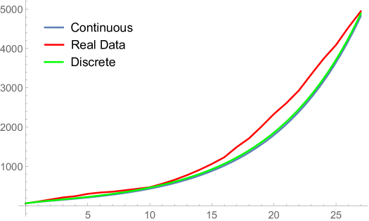
Figure 1: Cumulative cases of infection by HIV/AIDS in Cape Verde in the period from 1987 (year 0) to 2014 (year 27): real data (red); prediction from the continuous-time SICA model (1.1) (blue); and prediction from our discrete-time SICA model (3.1) (green).

To illustrate the global stability of the endemic equilibrium (EE), predicted by our Theorem 7, we consider different initial conditions borrowed from [5], from different regions of the plane:

$$\begin{split}\text{(SD1,ID1,CD1,AD1)}&=(S_{0},I_{0},C_{0},A_{0}),\\ \text{(SD2,ID2,CD2,AD2)}&=(S_{0}/2,I_{0}+S_{0}/2,C_{0}+10^{4},A_{0}+4\times 10^{4}),\\ \text{(SD3,ID3,CD3,AD3)}&=(S_{0}/3,I_{0},C_{0}+4\times 10^{4},A_{0}+S_{0}/3),\\ \text{(SD4,ID4,CD4,AD4)}&=(3S_{0}/2,I_{0}+S_{0}/4,C_{0}+5\times 10^{5},A_{0}+S_{0}/5).\end{split}$$ (4.2)

The obtained results are given in Figure 2.

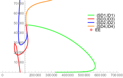
(a) HIV-infected individuals with no clinical symptoms ($I$) versus Susceptible individuals ($S$).

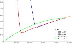
(b) HIV-infected individuals with AIDS ($A$) versus HIV-infected individuals under treatment ($C$).

Figure 2: Illustration of the fact that the endemic equilibrium point $(S^{\ast},I^{\ast},C^{\ast},A^{\ast})=(145276,48136.4,461146,3580.57)$ of the discrete-time SICA model (3.1) is globally asymptotically stable. This is in agreement with Theorem 7, since $\mathcal{R}_{0}=4.5304>1$.

5 Conclusions

In this work, we proposed a discrete-time SICA model, using Mickens’ nonstandard finite difference (NSFD) scheme. The elementary stability was studied and the global stability of the equilibrium points proved. Finally, we made some numerical simulations, comparing our discrete model with the continuous one. For that, we have used the same data, following the case study of Cape Verde. Our conclusion is that the discrete model can be used with success to describe the reality of Cape Verde, as well as to properly approximate the continuous model. All our simulations have been done using the numerical computing environment Mathematica, version 12.1, running on an Apple MacBook Pro i5 2.5 GHz with 16Gb of RAM. The solutions of the models were found in “real time”.

Mickens was a pioneer in NSFD schemes. Throughout the years, other NSFD schemes were developed. Roughly speaking, different Mickens-type methods differ on the denominator functions and the discretization, depending on concrete conditions that the continuous model under study must satisfy. In [20], the incidence rate is combined, while in [21] all parameters are constant. Other types of NSFD are presented, e.g., in [22, 23, 24, 25], which can be used if the system satisfy some conditions and a suitable denominator function is constructed. For such schemes, the incidence functions are different from ours. In [23], for example, it is fundamental to rewrite the system and the discretization method and the denominator function are different from the ones we use here. The article [24] uses the same approach of [23] and the model has a bilinear incidence function. Positive and elementary stable nonstandard finite-difference methods are also considered in [25]. Mickens set the field, but several different authors developed and are developing other related discretization methods. For the SICA model, however, as we have shown, a new NSFD scheme is not necessary and the standard Mickens’ method provides a well posed discrete-time model with excellent results, without the need to impose additional conditions to the model.

Conflict of interest

The authors declare that they have no conflicts of interest.

References

• 1 [10.1140/epjp/s13360-020-00839-1] S. M. Salman, A nonstandard finite difference scheme and optimal control for an HIV model with Beddington-DeAngelis incidence and cure rate, Eur. Phys. J. Plus, 135 (2020), 1–23.
• 2 (MR4154927) [10.1016/j.cam.2020.113203] S. M. Salman, Memory and media coverage effect on an HIV/AIDS epidemic model with treatment, J. Comput. Appl. Math., 385 (2021), 113203.
• 3 (MR4027867) [10.1080/17513758.2019.1683630] A. M. Elaiw, M. A. Alshaikh, Global stability of discrete virus dynamics models with humoural immunity and latency, J. Biol. Dyn., 13:1 (2019), 639–674.
• 4 (MR3392642) [10.3934/dcds.2015.35.4639] C. J. Silva, D. F. M. Torres, A TB-HIV/AIDS coinfection model and optimal control treatment, Discrete Contin. Dyn. Syst., 35 (2015), 4639–4663. \arXiv1501.03322
• 5 [10.1007/978-3-030-49896-2_6] C. J. Silva, D. F. M. Torres, On SICA Models for HIV Transmission, in Mathematical Modelling and Analysis of Infectious Diseases, Studies in Systems, Decision and Control 302, Springer Nature Switzerland AG, (2020), 155–179. \arXiv2004.11903
• 6 [10.1016/j.ecocom.2016.12.001] C. J. Silva, D. F. M. Torres, A SICA compartmental model in epidemiology with application to HIV/AIDS in Cape Verde, Ecol. Complexity, 30 (2017), 70–75. \arXiv1612.00732
• 7 (MR3808514) [10.1016/j.aml.2018.05.005] J. Djordjevic, C. J. Silva, D. F. M. Torres, A stochastic SICA epidemic model for HIV transmission, Appl. Math. Lett., 84 (2018), 168–175. \arXiv1805.01425
• 8 [10.1140/epjp/s13360-020-01013-3] A. Boukhouima, E. M. Lotfi, M. Mahrouf, S. Rosa, D. F. M. Torres, N. Yousfi, Stability analysis and optimal control of a fractional HIV-AIDS epidemic model with memory and general incidence rate, Eur. Phys. J. Plus, 136 (2021), 1–20. \arXiv2012.04819
• 9 (MR3895105) [10.1016/j.nahs.2018.12.005] M. Bohner, S. Streipert, D. F. M. Torres, Exact solution to a dynamic SIR model, Nonlinear Anal. Hybrid Syst., 32 (2019), 228–238. \arXiv1812.09759
• 10 (MR4091761) [10.3390/mca25010001] C. Campos, C. J. Silva, D. F. M. Torres, Numerical optimal control of HIV transmission in Octave/MATLAB, Math. Comput. Appl., 25 (2020), 20 pp. \arXiv1912.09510
• 11 [10.1007/s00500-019-04645-5] S. Nemati, D. F. M. Torres, A new spectral method based on two classes of hat functions for solving systems of fractional differential equations and an application to respiratory syncytial virus infection, Soft Comput., 25 (2021), 6745–6757. \arXiv1912.11919
• 12 (MR1402909) A. M. Stuart, A. R. Humphries, Dynamical Systems and Numerical Analysis, Cambridge University Press, New York, 1996.
• 13 (MR1275372) R. E. Mickens, Nonstandard finite difference models of differential equations, World Scientific Publishing Co., Inc., River Edge, NJ, 1994.
• 14 (MR1919887) [10.1080/1023619021000000807] R. E. Mickens, Nonstandard finite difference schemes for differential equations, J. Difference Equation Appl., 8 (2002), 823–847.
• 15 (MR2739251) [10.1016/j.mcm.2010.07.026] S. M. Garba, A. B. Gumel, J. M-S. Lubuma, Dynamically-consistent non-standard finite difference method for an epidemic model, Math. Comput. Modelling, 53 (2011), 131–150.
• 16 (MR3733771) [10.4134/BKMS.b160240] S. Liao, W. Yang, A nonstandard finite difference method applied to a mathematical cholera model, Bull. Korean Math. Soc., 54 (2017), 1893–1912.
• 17 (MR2173250) [10.1080/10236190412331334527] R. E. Mickens, Dynamic consistency: a fundamental principle for constructing nonstandard finite difference schemes for differential equations, J. Difference Equation Appl., 11 (2005), 645–653.
• 18 (MR4183276) [10.1080/10236198.2020.1812594] A. K. Verma, S. Kayenat, An efficient Mickens’ type NSFD scheme for the generalized Burgers Huxley equation, J. Difference Equation Appl., 26 (2020), 1213–1246.
• 19 (MR4128034) [10.1007/s40314-020-01257-w] A. K. Verma, S. Kayenat, Applications of modified Mickens-type NSFD schemes to Lane-Emden equations, Comput. Appl. Math., 39 (2020), 1–25.
• 20 (MR4141413) [10.1080/10236198.2020.1792892] R. Anguelov, T. Berge, M. Chapwanya, J. K. Djoko, P. Kama, J. M. S. Lubuma, et al., Nonstandard finite difference method revisited and application to the Ebola virus disease transmission dynamics, J. Difference Equation Appl., 26 (2020), 818–854.
• 21 (MR3093413) [10.1016/j.cam.2013.04.042] R. Anguelov, Y. Dumont, J. M. S. Lubuma, M. Shillor, Dynamically consistent nonstandard finite difference schemes for epidemiological models, J. Comput. Appl. Math., 255 (2014), 161–182.
• 22 (MR3575285) [10.1016/j.matcom.2016.04.007] D. T. Wood, H. V. Kojouharov, D. T. Dimitrov, Universal approaches to approximate biological systems with nonstandard finite difference methods, Math. Comput. Simul., 133 (2017), 337–350.
• 23 (MR3316778) [10.1080/10236198.2014.997228] D. T. Wood, D. T. Dimitrov, H. V. Kojouharov, A nonstandard finite difference method for $n$-dimensional productive-destructive systems, J. Difference Equation Appl., 21 (2015), 240–254.
• 24 (MR2854820) [10.1080/10236191003781947] D. T. Dimitrov, H. V. Kojouharov, Dynamically consistent numerical methods for general productive-destructive systems, J. Difference Equation Appl., 17 (2011), 1721–1736.
• 25 (MR2316130) D. T. Dimitrov, H. V. Kojouharov, Nonstandard numerical methods for a class of predator-prey models with predator interference, Electron. J. Differ. Equation Conf., 15 (2007), 67–75.
• 26 (MR2128146) S. Elaydi, An Introduction to Difference Equations, third edition, Springer, New York, 2005.
• 27 (MR1950747) [10.1016/S0025-5564(02)00108-6] P. van den Driessche, J. Watmough, Reproduction numbers and sub-threshold endemic equilibria for compartmental models of disease transmission, Math. Biosci. 180 (2002), 29–48.
• 28 (MR2310267) [10.1002/num.20198] R. E. Mickens, Calculation of denominator functions for nonstandard finite difference schemes for differential equations satisfying a positivity condition, Numer. Methods Partial Differential Equations 23 (2007), 672–691.
• 29 (MR3125375) [10.1016/j.camwa.2013.06.011] R. E. Mickens, T. M. Washington, NSFD discretization of interacting population models satisfying conservation laws, Comput. Math. Appl., 66 (2013), 2307–2316.
• 30 (MR2202966) [10.1016/j.cam.2005.04.003] D. T. Dimitrov, H. V. Kojouharov, Positive and elementary stable nonstandard numerical methods with applications to predator-prey models, J. Comput. Appl. Math., 189 (2006), 98–108.
• 31 (MR2447189) [10.1080/10236190802332308] L. J. S. Allen, P. van den Driessche, The basic reproduction number in some discrete-time epidemic models, J. Difference Equation Appl., 14 (2008), 1127–1147.
• 32 República de Cabo Verde, Rapport de Progrès sur la riposte au SIDA au Cabo Verde-2015, Comité de Coordenação do Combate à SIDA (2015).
• 33 World Bank Data, World Development Indicators, Available from: http://data.worldbank.org/country/cape-verde.
• 34 (MR2401283) [10.3934/mbe.2008.5.145] O. Sharomi, C. N. Podder, A. B. Gumel, B. Song, Mathematical analysis of the transmission dynamics of HIV/TB confection in the presence of treatment, Math. Biosci. Eng., 5 (2008), 145–174.
• 35 (MR2544634) [10.1007/s11538-009-9423-9] C. P. Bhunu, W. Garira, Z. Mukandavire, Modeling HIV/AIDS and tuberculosis coinfection, Bull. Math. Biol., 71 (2009), 1745–1780.
• 36 [10.1038/387188a0] A. S. Perelson, P. Essunger, Y. Cao, M. Vesanen, A. Hurley, K. Saksela, et al., Decay characteristics of HIV-1-infected compartments during combination therapy, Nature, 387, (1997), 188–191.
• 37 M. Zahlen, M. Egger, Progression and mortality of untreated HIV-positive individuals living in resources-limited settings: Update of literature review and evidence synthesis, Report on UNAIDS obligation no. HQ/05/422204 (2006).
• 38 World Bank Data, Population, total–Cabo Verde, Available from: http://data.worldbank.org/indicator/SP.POP.TOTL?locations=CV.
• 39 [10.1056/NEJMoa1105243] M. S. Cohen, Y. Q. Chen, M. McCauley, et al., Prevention of HIV-1 infection with early antiretroviral therapy, N. Engl. J. Med, 365 (2011), 493–505.
• 40 [10.1097/MD.0000000000004398] J. Del Romero, Natural conception in HIV-serodiscordant couples with the infected partner in suppressive antiretroviral therapy: A prospective cohort study, Medicine, 95 (2016), e4398.
• 41 [10.1016/S0140-6736(08)61115-0] D. P. Wilson, M. G. Law, A. E. Grulich, D. A. Cooper, J. M. Kaldor, Relation between HIV viral load and infectiousness: a model based analysis, Lancet, 372 (2008), 314–320.