Ising Machines’ Dynamics and Regularization for Near-Optimal Large and Massive MIMO Detection

Abstract

Optimal MIMO detection is one of the most computationally challenging tasks in wireless systems. We show that new analog computing approaches, such as Coherent Ising Machines (CIMs), are promising candidates for performing near-optimal MIMO detection. We propose a novel regularized Ising formulation for MIMO detection that mitigates a common error floor issue in the naive approach and evolve it into a regularized, Ising-based tree search algorithm that achieves near-optimal performance. Massive MIMO systems use a large number of antennas at the base station to allow a linear detector to achieve near-optimal performance. However, this comes at the cost of overall throughput, which could be improved by supporting more users with the same number of antennas. By means of numerical simulation using the Rayleigh fading channel model, we show that in principle, a MIMO detector based on a high-speed Ising machine (such as a CIM implementation optimized for latency) would allow more transmitter antennas (users) and thus increase the overall throughput of the cell by a factor of two or more for massive MIMO systems. Our methods create an opportunity to operate wireless systems using more aggressive modulation and coding schemes and hence achieve high spectral efficiency: for a $16\times 16$ MIMO system, we estimate around 2.5$\times$ more throughput in the mid-SNR regime ($\approx 12$ dB) and 2$\times$ more throughput in the high-SNR regime ($>$20 dB) as compared to the industry standard, a Minimum-Mean Square Error (MMSE) linear decoder.

I Introduction

Wireless technologies have recently undergone tremendous growth in terms of supporting more users and providing higher spectral efficiency, with the next generation of cellular networks planning to support massive machine-to-machine communication [1], large IoT networks [2], and unprecedented data rates [3]. The number of mobile users and data usage is rapidly increasing [4], and while data traffic has been predominantly downlink, the volume of uplink traffic is becoming ever higher [5] due to the emergence of interactive services and applications. The problem of optimal and efficient wireless signal detection in a Multiple-Input, Multiple-Output (MIMO) system is central to this rapid growth and has been a key interest of network designers for several decades. While the optimal Maximum Likelihood (ML) detector is well known, it attempts to solve an NP-Hard problem [6] exactly, and so its implementation is usually impractical and infeasible for real-world systems. These computational challenges have prompted network designers to seek optimized implementations such as the Sphere Decoder [7, 8], or sub-optimal approximations with polynomial complexity, including linear detectors like the Minimum Mean Square Error decoder (MMSE) [9], and successive interference cancellation (SIC) [10, 11], approximate tree search algorithms like the Fixed Complexity Sphere Decoder [12] and Lattice-reduction based algorithms [13]. However, even today, practical methods that achieve near-optimal performance for systems with large numbers of both users and antennas are lacking [6].

Instead, Massive MIMO systems [14, 15], where the number of base station antennas is much larger than the number of users, have emerged as the dominant solution to the poor bit error performance of practically-feasible MIMO detectors. Such systems have extremely well-conditioned channels, and hence even linear detectors like MMSE achieve near-optimal BER performance [16, 17, 18]. While this enables very low BER without any significant computational load, unfortunately, it comes at the cost of extreme under-utilization of available radio resources, as we can potentially support much larger spectral efficiency by concurrently serving more uplink users (up to the number of base station antennas). The existence of a near-optimal MIMO detector with practical complexity for large MIMO systems would enable the expansion of massive MIMO systems to serve more users by having a base station antenna-user ratio of less than two, improving the overall uplink throughput of the system several-fold.

In the Computer Architecture and Physics communities, the last decade has seen a rise of a novel class of analog computers that use the dynamics of a physical system to heuristically find solutions to optimization problems framed as instances of the Ising model, one of the most studied frameworks for magnetism in statistical mechanics. These methods include Quantum Annealing [19, 20], Coherent Ising Machines (optical or opto-electronic systems) [21, 22, 23, 24, 25, 26], and Oscillator-based Ising Machines [27]. These already show promise as practical computational structures for addressing some NP-hard problems arising in practical applications. However, recent starting work [28, 29] on the MIMO detection leveraging a straightforward mapping of ML-MIMO decoding problem to the Ising model experiences an error floor in the bit error rate (BER) versus the signal-to-noise ratio (SNR) characteristics.

In this paper, we observe that this error floor is present in the regime of practical deployment for MIMO detection. More specifically, in the regime relevant for real systems (uncoded BER of $10^{-3}-10^{-6}$), even if we dismiss the limitations of non-idealized physics-based Ising solvers, depending on the SNR, there are many interesting scenarios in which they would not serve as good MIMO detectors in practical systems if the known Ising formulation of the ML-MIMO detection problem is used. Hence we propose a novel regularized Ising formulation of the ML-MIMO problem, using a low-complexity approximation (see Fig. 1 for an overview of our decoder architecture).

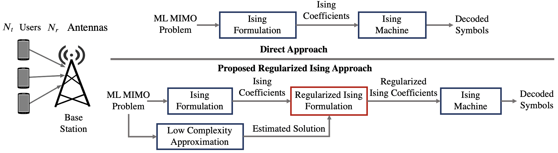
Figure 1: Uplink Maximum Likelihood MIMO detection (ML-MIMO) using Ising Machines, illustrating the differences between the proposed regularised Ising approach and the direct application of the Ising formulation.

This new formulation leads us to propose two MIMO detection algorithms, that can in principle, provide near-optimal MIMO detection on Ising machines in the relevant SNR regime (an uncoded BER of $10^{-3}$-$10^{-6}$). We propose Regularised Ising MIMO (RI-MIMO), which is based on the regularised Ising approach, and show that it is asymptotically optimal and can achieve near-optimal performance within practical complexities. We further evolve RI-MIMO into Tree search with RI-MIMO (TRIM) that allows us to achieve better performance when the complexity of the underlying MIMO detection problem increases with higher-order modulations. Finally, we estimate how a physical implementation of a Coherent Ising machine could employ these algorithms to bridge the gap between optimality and efficiency in MIMO detection and may realize a near-optimal MIMO detector, meeting the cellular-system-complexity and timing requirements of practical scenarios, years before quantum-annealing technology would reach the necessary maturity [30, 31].

The rest of the paper is organized as follows. Section II provides a survey of the existing state-of-the-art to solve ML-MIMO and elaborates on why incremental improvement would not be sufficient for meeting the processing requirements of important scenarios of future cellular systems. Section III describes the MIMO system model and the reduction of the ML-MIMO problem to an Ising optimization problem. Section IV is a primer on Coherent Ising Machines. Section V describes our novel Ising formulation and the proposed MIMO detection algorithms (RI-MIMO and TRIM). Section VI contains an extensive evaluation of BER and spectral efficiency of our methods in various scenarios. We show that our techniques mitigate the error floor problem and can achieve the same BER as the Sphere Decoder for $16\times 16$ MIMO with BPSK modulation. We study the impact of practical constraints, like finite precision, on the performance of CIM for MIMO detection and show that regularized Ising approach is more resilient to finite precision, and five bits of precision lead to the same BER as floating-point precision, for a $16\times 16$ MIMO with BPSK modulation. We perform extensive empirical experimentation for parameter tuning. We show that for higher-order modulations, our methods provide a 10-15 dB gain over the MMSE receiver. We evaluate our methods with Adaptive Modulation and Coding (AMC) and show that our methods can achieve around 2.5$\times$ more throughput in the mid-SNR regime ($\approx$12 dB) and 2$\times$ more throughput in high-SNR regime($>$20 dB) than the industrially-viable MMSE decoding. We evaluate the spectral efficiency of several massive MIMO systems ($4\times 16$, $8\times 16$, $8\times 64$ and, $16\times 64$) and show that TRIM improves their spectral efficiency and allow us to add more users to the system, resulting in a $>2\times$ gain in overall cell throughput. Finally, we conclude with future work in Section VII.

II Related Work

The challenge of achieving good error performance at a practically feasible computational complexity has troubled network designers for decades. The state-of-the-art cellular technologies, like LTE and 5G NR, aim to provide very high data rates and extremely low latency [32, 33], which makes the timing constraints on MIMO detection increasingly strict.

The Maximum Likelihood MIMO detection (ML-MIMO) has been a key problem of interest for wireless systems for several decades. The Sphere Decoder [7, 8] (SD) is a reference algorithm to solve this problem, which performs an optimized, pruned tree search. Its average computational complexity is still exponential [34], so its deployment is practically infeasible for MIMO systems with a large number of users due to the strict timing requirements of state-of-the-art wireless systems like 5G NR. Consequently, there has been a large number of variations over the baseline SD algorithm, with the objective to develop approximate algorithms with polynomial complexity that could be utilized in the real world. For instance, the Fixed Complexity Sphere Decoder [12] (FSD) is a polynomial-time approximation to the sphere decoder that aggressively prunes the search tree. In practice, wireless network designers resort to simpler methods like linear detectors (MMSE), which perform channel inversion, or successive interference cancellation (SIC) based techniques [10, 11] that focus on decoding each user sequentially while canceling inter-user interference. Given the practical importance of MMSE and SIC, many techniques have been put forward to advance their performance, including Lattice Reduction (LR), which involves pre-processing the channel to produce a reduced lattice basis [13]. There is a large volume of literature on finding a practically feasible approximation to ML-MIMO detection problem [35, 36, 37, 38], which provide good BER performance, employing search space reduction, iterative improvement of a linear estimate, or mathematical methods like Lattice Reduction [39]. In [40], the authors use the L2 norm of the solution to regularize the fixed complexity sphere decoder to deal with a rank deficient channel in an OFDM/SDMA uplink, and in [41], the authors use the MMSE estimate to determine the search radius during sphere decoding. In [42], authors explore L1 and L2 regularisation to improve the performance of lattice sphere decoding. In [43], authors propose a dead-zone penalty and infinity-norm-based regularisation to improve the performance of the MMSE detector. Regularised Lattice Decoding, like the MMSE-regularised lattice decoding, penalizes deviations from origin to mitigate the out-of-bound symbol events in lattice reduction-based MIMO detection [44]. In [44], authors propose a Lagrangian Dual relaxation for ML MIMO detection and generalize the regularised lattice decoding techniques. Regularisation techniques are also widely used in Machine Learning to prevent over-fitting [45]. Many of these works can achieve near-optimal performance for small systems; however, as the number of users and number of antennas at the base station increase, they require an exponential increase in computation time (to maintain near-optimal behavior), or their performance becomes progressively worse.

While we discuss Coherent Ising Machines in this paper, there are a number of other promising Ising-machine technologies [46], including quantum annealing [47, 48], photonic Ising machines besides CIMs [49, 50, 51, 52], digital-circuit Ising solvers [53, 54, 55, 56, 57], bifurcation machines [58], oscillation based Ising machines [27], and memristor and spintronic Ising machines [59, 60, 61].

The application of Quantum Annealing (QA) and Ising machines to MIMO detection is starting to be investigated in the last couple of years [62] and has shown promising results. The QuAMax MIMO detector [28] leverages quantum annealing for MIMO detection. A classical-quantum hybrid approach to QA-based ML-MIMO was proposed in [63]. QA has shown promising results for other tough computational problems in wireless systems like Vector Perturbation Precoding [64]. In [29], authors explore the use of Parallel Tempering for Ising-based MIMO detection (ParaMax), improving the performance of QuAMax. However, both QuAMax and ParaMax suffer from the aforementioned bit error floor, which is addressed in our work. In [65], the authors explore the use of Oscillator based Ising machines for MU-MIMO decoding. However, their evaluation is limited to only a single Massive MIMO, $16\times 64$ 4-QAM scenario, for which simple linear decoders like MMSE can achieve near-optimal performance, and doesn’t explore performance across modulations, varying number of users, and a varying number of runs per instance of the Ising problem. Unlike [65], we explore the tough large MIMO scenarios, like $16\times 16$, $20\times 20$, and $24\times 24$ for BPSK modulation and $12\times 12$, $16\times 16$ for 4-QAM, and 16-QAM modulations, where the number of users is equal to the number of antennas at the BS, and linear detectors have a terrible BER. We demonstrate that our methods provide significant gains and also present, to the best of our knowledge, the first empirical evaluation of spectral efficiency and show that our methods can be used to expand massive MIMO systems ($4\times 16$, $8\times 16$, $16\times 64$ with BPSK, 4-QAM and 16-QAM modulations) to include more users with more than $2\times$ enhancement in the overall cell throughput.

MIMO System	ETH SD Processing	Parallel ASIC
	Throughput (Mbps)	requirement for LTE
4x4, 16 QAM	20	7
6x6, 16 QAM	16	13
8x8, 16 QAM	11.17	24
16x16, 16 QAM	1.8	300
32x32, 16 QAM	0.022	$\approx 49000$
64x64, 16 QAM	$16.7\times 10^{-7}$	$\approx$1.3 billion

TABLE I: Parallel ASIC requirement to meet LTE processing requirements with ETH SD.

There are several FPGA/ASIC implementations of the Sphere Decoder in the literature. The ETH SD is known to be one of the most optimized implementations of the Sphere Decoder algorithm. The ETH SD can achieve a high processing throughput of 20 Mbps with its one cycle per-node architecture for a $4\times 4$ MIMO system at 8 dB SNR, with a single ASIC processing element. To estimate the performance of ETH SD for larger systems like $16\times 16$ MIMO with 16-QAM constellation, we rely on the fact that the Sphere Decoding algorithm is known to have exponential average complexity, unless we operate sufficiently under the capacity or have high SNR [34, 66]. As described in [34], the lower bound on the average number of nodes visited by the sphere decoder still scales exponentially with the number of users in the system $m$. Using the data in [34], we can approximately extrapolate the results of ETH SD by linearly extrapolating the logarithm of the average number of nodes visited reported in the paper. We obtain that for $16\times 16$ MIMO, ETD SD will visit approximately 814 nodes, on average. Since the processing time of ETH SD is proportional to the number of nodes visited (due to its one cycle per node architecture), ETH SD will require approximately $45\times$ more time to process each $16\times 16$ MIMO problem, leading to a deterioration in its processing throughput to a mere 1.8 Mbps, which is not sufficient for the current wireless technologies. As per the LTE specifications, a typical LTE deployment with 10 MHz bandwidth and 15KHz sub-carrier spacing produces 8400 MIMO detection problems (corresponding to 14 OFDM symbols per sub-frame and 600 sub-carriers) every 1ms. Assuming $16\times 16$ MIMO and 16 QAM modulation (same as ETH SD results), it requires a processing throughput of $\approx 538$ Mbps. Hence in order to meet the processing requirements, the base station will need to put approximately 300 FPGA/ASIC implementations of ETH SD in parallel. We use similar reasoning to estimate performances in Table I, illustrating that current silicon-based implementation can only support MIMO sizes like $8\times 8$ with less than 25 parallel implementations, but larger systems like $64\times 64$ will require a billion parallel instances of ETH SD, which is impractical. As a result, practical deployments of large MIMO systems end up using computationally efficient linear detectors like Zero Forcing or MMSE, but their BER performance is significantly worse. The inefficient scaling FPGA implementations of Sphere Decoder and unacceptable BER performance of linear detectors prompt us to explore novel hardware/algorithmic solutions.

III MIMO Systems, Ising problems and Maximum Likelihood Detection

In this section, we will describe the MIMO system model, the MIMO Maximum Likelihood Detection (ML-MIMO) problem, and the transformation between the ML-MIMO problem and its equivalent Ising problem.

Consider the UL transmission in a MIMO system [67] with $N_{r}$ antennas at the base station (BS) and $N_{t}$ users, each with a single antenna. $\mathbf{x_{o}}=\{x_{1},x_{2},...x_{N_{t}}\}^{T}$ is the transmit vector where $x_{i}$ is the symbol transmitted by user $i$. $\mathbf{y}=\{y_{1},y_{2},...y_{N_{r}}\}^{T}$ is the received vector where $y_{j}$ is the signal received by antenna $j$. Each $x_{i}$ is a complex number drawn from a fixed constellation $\Omega$. The channel between user $j$ and receive antenna $i$ is expressed as a complex number $h_{ij}$ that represents the channel’s attenuation and phase shift of the transmitted signal $x_{j}$. Let $\mathbf{H}$ denote the complex-valued channel matrix,

$$\mathbf{y}=\mathbf{H}\mathbf{x_{o}}+\mathbf{n},$$ (1)

where $\mathbf{n}$ denotes Additive White Gaussian Noise (AWGN). With AWGN, the optimal receiver is the Maximum Likelihood receiver [8] which is given by

$$\mathbf{\hat{x}_{ML}}=\min_{\mathbf{x}\in\Omega^{N_{t}}}\|\mathbf{y}-\mathbf{H}\mathbf{x}\|^{2}$$ (2)

An Ising optimization problem [68, 69] is quadratic unconstrained optimization problem over $N$ spin variables, as follows:

$$\min_{s_{1},s_{2},...s_{N}}-\sum_{i=1}^{N}h_{i}s_{i}-\sum_{i\neq j}J_{ij}s_{i}s_{j}=\min_{\mathbf{s}\in\{-1,1\}^{N}}-\mathbf{h}^{T}\mathbf{s}-\mathbf{s}^{T}\mathbf{J}\mathbf{s},$$ (3)

where each spin variable $s_{i}\in\{-1,1\}$, or in its vector form (RHS) $\mathbf{s}=\{s_{1},s_{2},...s_{N}\}$, where all diagonal entries of the matrix $\mathbf{J}$ are zeros.

The minimization problem expressed in Eq. 2 can be equivalently converted into Ising form by expressing $\mathbf{x}$ using spin variables. The first step is derive a real valued equivalent of Eq. 1, which is obtained by the following transformation,

$$\mathbf{\tilde{H}}=\left[{\begin{array}[]{cc}Re(\mathbf{H})&-Im(\mathbf{H})\\ Im(\mathbf{H})&Re(\mathbf{H})\\ \end{array}}\right],\text{~{}}$$ (4)

$$\mathbf{\tilde{y}}=\left[{\begin{array}[]{c}Re(\mathbf{y})\\ Im(\mathbf{y})\\ \end{array}}\right],\text{~{}}\mathbf{\tilde{x}}=\left[{\begin{array}[]{c}Re(\mathbf{x})\\ Im(\mathbf{x})\\ \end{array}}\right],$$ (5)

The ML receiver described in Eq. 2 has the same expression under the transformation and the optimization variable $\mathbf{\tilde{x}}$ is real valued. Let us say $\mathbf{\tilde{x}}$ has $N$ elements, which are drawn from a square M-QAM constellation, then each element of the optimization variable $\mathbf{\tilde{x}}$ takes integral values in the range $\Omega_{r}=\{-\sqrt{M}+1,-\sqrt{M}+3,...\sqrt{M}-1\}$. The number of bits needed to express $\Omega_{r}$ are given by $r_{b}=\lceil\log_{2}(\sqrt{M})\rceil$. let $\mathbf{s}$ be an $N*r_{b}\times 1$ spin vector such than each element of $\mathbf{s}$ can take values $\{-1,1\}$. Then, element $j$ of $\mathbf{\tilde{x}}$ can be represented using $r_{b}$ spin variables $\{s_{j},s_{j+N}...s_{j+(r_{b}-1)N}\}$,

$$\tilde{x}_{j}=\sum_{i=1}^{r_{b}}2^{r_{b}-i}(s_{j+(i-1)N}+1)-(\sqrt{M}-1)$$ (6)

Let us define the transform matrix $\mathbf{T}=\left[2^{r_{b}-1}\mathds{I}_{N}\text{~{}~{}~{}}2^{r_{b}-2}\mathds{I}_{N}\text{~{}}...\text{~{}}\mathds{I}_{N}\right]$, then $\mathbf{\tilde{x}}$ can be expressed as,

$$\mathbf{\tilde{x}}=\mathbf{T}(\mathbf{s}+\bar{\mathds{1}}_{N*r_{b}})-(\sqrt{M}-1)\bar{\mathds{1}}_{N}$$ (7)

For a rectangular QAM constellation, like BPSK, the $Re(\mathbf{x})$ and $Im(\mathbf{x})$ in Eq 5 have different range and Eq. 6 can be accordingly modified to construct the transform matrix $T$. We substitute Eq. 7 in the real valued maximum likelihood problem and simplify to obtain the ising formulation for ML receiver. Let $\mathbf{z}=\mathbf{\tilde{y}}-\mathbf{\tilde{H}}\mathbf{T}\bar{\mathds{1}}_{N*r_{b}}+(\sqrt{M}-1)\mathbf{\tilde{H}}\bar{\mathds{1}}_{N}$, then the Ising problem for ML-MIMO receiver is described by,

$$\mathbf{h}=2*\mathbf{z}^{T}\mathbf{\tilde{H}}\mathbf{T}\text{,~{}~{}~{}~{}}\mathbf{J}=-\textit{zeroDiag}(\mathbf{T}^{T}\mathbf{\tilde{H}}^{T}\mathbf{\tilde{H}T}),$$ (8)

where $\textit{zeroDiag}(\mathbf{W})$ sets the diagonal elements of matrix $W$ to zero. We further scale the problem such that all the coefficients lie in $[-1,1]$. The Ising solution can be converted to real valued ML solution using Eq. 7, which can be then converted to the complex valued solution for the original problem described in Eq. 2 by inverting the transform described by Eq. 5.

IV Coherent Ising Machines (CIM)

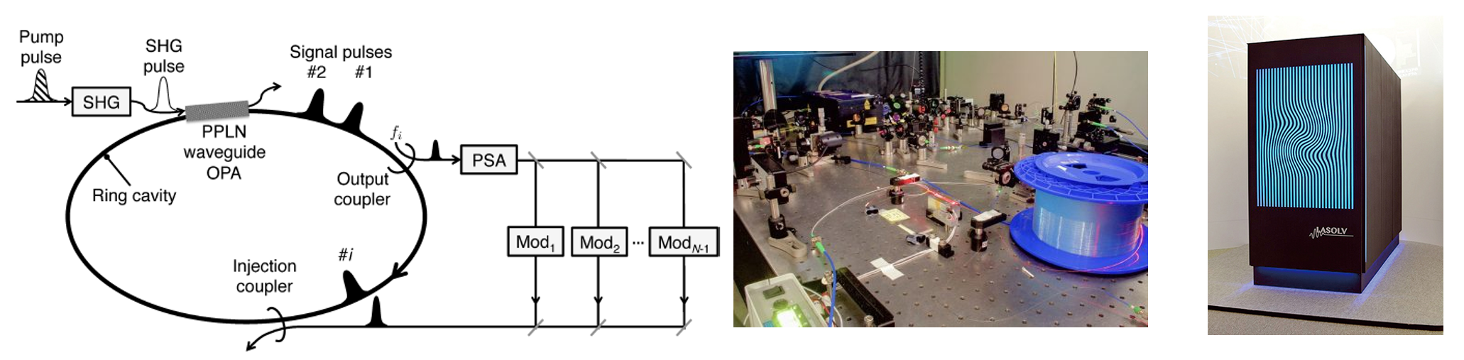
Figure 2: Left: Schematic architecture of a CIM based on time-multiplexed optical spins represented by pulses, coupled by optical delay lines (Figure from Ref. [25]). Center: photo of an experimental implementation of a CIM at Stanford University (Figure from [70]) Right: commercial CIM product by NTT (LASOLV^TM, image from https://www.rd.ntt/e/research/JN20191127_h.html)

In simple terms, an Ising Machine can be described as a module that takes an Ising Problem (Eq. 3) as input and outputs a candidate solution, according to an unknown probability distribution that depends on a few parameters. We refer to a single, independent run on the Ising Machine as an ”anneal”, borrowing nomenclature from the simulated/quantum-annealing methods. After each run, the machine is reset. A common approach is to run several samples of a single Ising problem instance and then return the best-found solution (the ”ground state”) in the sample.

Coherent Ising Machines (CIMs), as originally conceived [22, 23, 24], implement the search for the ground state of an Ising problem by using an optical artificial spin network. Their baseline architecture encodes the Ising spins into a train of time-resolved, phase-coherent laser pulses traveling on an optical fiber loop, undergoing controlled interference between all pairs of wavepackets, as illustrated in Fig. 2. The phase dynamics of the pulses is governed by the presence of a non-linear element in the form of a degenerate-optical-parametric-oscillator (DOPO). For the purpose of our work, this version of the CIM can be modeled using a system of stochastic differential equations [21]. In this work, we will use a model of the CIM that describes its continuous-time limit evolution neglecting quantum effects, which has been proven to be fitting the experiments of multiple devices and represents a baseline setup for more sophisticated embodiments. Following Ref. [25], the in-phase ($c_{i}$) and quadrature ($q_{i}$) components of each signal-variable can be modeled using the following differential equations:

$$dc_{i} = [(-1+p-c_{i}^{2}-q_{i}^{2})c_{i}+C\sum_{j}J_{ij}c_{j}]dt$$ (9)

$$+ \frac{1}{A_{s}}\sqrt{c_{i}^{2}+q_{i}^{2}+\frac{1}{2}}dW_{1}$$

$$dq_{i} = (-1-p-c_{i}^{2}-q_{i}^{2})q_{i}dt+\frac{1}{A_{s}}\sqrt{c_{i}^{2}+q_{i}^{2}+\frac{1}{2}}dW_{2}$$

where the normalized pump rate ($p$) are CIM parameters that relates to the laser used in the machine and can be tuned easily. The constant C is typically fixed by design considerations (mostly by the power transmission coefficient and the laser saturation amplitude). $J_{ij}$ is the Ising coupling coefficient from the $j^{th}$ pulse to the $i^{th}$ pulse, which is programmable. The stochasticity is introduced through $dW_{1}$ and $dW_{2}$, which are independent Gaussian-noise processes. The variable $t$ is time (normalized with respect to the photon decay rate). An Ising problem with the spin-spin-coupling matrix $J$ is encoded in the CIM by setting the optical couplings $\tilde{\zeta}_{ij}\propto J_{ij}$. The anneal consists of pumping energy into the system by gradually varying $p$. Heuristically this is implemented in a schedule at a speed that is some monotonic function of $N$. The solution to the Ising problem is read out at the end of the anneal by measuring the in-phase component of each DOPO $c_{i}$, and interpreting the sign of each as a spin value $s_{i}$, i.e. $s_{i}=\textrm{sign}(c_{i})$.

IV-A CIM Simulator

To enable the study of how an ideal CIM would perform on solving Ising instances related to the application at hand (MIMO detection), we implemented a software simulator of a CIM that integrates the differential equations described in Eqs. IV, using double precision numerics implemented in MATLAB. The annealing schedule consists in varying the pump parameter as $p(t)=2*\tanh(\frac{2t}{N})$. For the purpose of numerical integration, $dt=0.01$ and the total anneal time is $128*dt$, which corresponds to 128 steps of numerical integration). In both numerics and experiments, we can also sample the state of the CIM at intermediate times (number of measurements $N_{m}$) to retrieve more candidate solutions for the programmed Ising problem and then select the best solution found; so each run actually evaluates $N_{m}=128$ candidate solutions. However, most of the time, the best solution corresponds to the one at the final measurement. Following the inspiration from design described in Ref. [25] we set $C=\sqrt{10}$. As the pump rate is gradually increased from 0 to 2, the amplitudes of DOPO pulses demonstrate a bifurcation and settle to either a positive (indicating spin +1) or a negative value (indicating spin -1).

V Design

In this section, we propose the RI-MIMO detector, based on our novel regularised Ising formulation of maximum-likelihood MIMO receiver, which mitigates the error floor problem. We use a single auxiliary spin variable to transform the Ising problem into a form compatible with CIMs. We finally propose TRIM, a novel tree search algorithm based on RI-MIMO, which enhances the performance for higher-order modulations.

V-A RI-MIMO: Regularized Ising-MIMO

As noted before, when we use Ising machines for MIMO detection, there is a finite probability of not returning the ground state of the problem, even at zero noise, and hence, we cannot decrease the BER beyond a certain limit (i.e., there is an ”error floor”). We can observe this error floor in existing works on ML-MIMO detection using a Quantum Annealer [28]. In this section, we present Regularized Ising-MIMO (RI-MIMO) that mitigates the error floor and provides significant performance enhancements.

V-A1 Regularization

The key idea is to add a regularisation term based on a low complexity estimate of the solution, which, as we will see later, will enhance the probability of finding the ground state of the Ising problem and hence improve the BER performance. The maximum likelihood MIMO receiver is given by Eq. 2. Let us say that we have a polynomial-time estimate (obtained by algorithms like MMSE or ZF) $\mathbf{x}_{P}$. Let $\mathbf{s}_{P}$ be the spin vector corresponding to $\mathbf{x}_{P}$ obtained from Eq. 7. We add to the Ising form a penalty term for deviations from the poly-time estimate, which would penalize non-optimal solutions in low noise scenarios, to obtain the following:

$$\mathbf{\hat{s}} = \min_{\mathbf{s}\in\{-1,1\}^{N}}-\mathbf{h}^{T}\mathbf{s}-\mathbf{s}^{T}\mathbf{J}\mathbf{s}+r(\rho,M,N_{t})\|\mathbf{s}-\mathbf{s}_{P}\|^{2}$$ (10)

$$= \min_{\mathbf{s}\in\{-1,1\}^{N}}-(\mathbf{h}+2r(\rho,M,N_{t})\mathbf{s}_{P})^{T}\mathbf{s}-\mathbf{s}^{T}\mathbf{J}\mathbf{s},$$

where $r(\rho,M,N_{t})$ is a regularization parameter dependent of the SNR, modulation and number of users. This style of regularisation falls in the class of generalized Tikhonov regularisation. We will look at the choice of $r(\rho,M,N_{t})$ in Section VI-C.

The RI-MIMO-$N_{a}$ algorithm is then defined as follows:

• Convert the ML-MIMO detection problem into the Ising form as described in Section III.

• Add the regularisation term as described by Eq. 10.

• Perform $N_{a}$ anneals using an Ising machine.

• Select the best solution from the candidate solutions generated by the Ising machine (one from each measurement times the number of anneals $N_{m}\times N_{a}$) and the MMSE solution.

In contrast to RI-MIMO, a trivial way to lower the error floor is to increase the number of runs per instance of the problem. However, each additional anneal increases the overall computation time as well. Another simple approach is to use a direct combination of Ising machine-based ML-MIMO and MMSE, where we select the best solution among those generated by the Ising machine and the MMSE solution. This removes the error floor but, at higher SNR, the reduction in BER is primarily due to the MMSE receiver and, as we will show later, our proposed techniques have much better BER performance.

V-B Solution of an Ising problem having access only to programmable quadratic couplings

Not all CIMs are designed to solve Ising problems containing a bias term ($\mathbf{h}^{T}\mathbf{s}$ in Eq. 3). In order to solve a general Ising problem using a CIM that does not natively support bias terms (although some, such as the implementation used in [23], do), we introduce an auxiliary spin variable $s_{a}$ and solve the following Ising problem:

$$\min_{s_{a},s_{1},s_{2},...s_{N}}-\sum_{i=1}^{N}h_{i}s_{i}s_{a}-\sum_{i\neq j}J_{ij}s_{i}s_{j},$$ (11)

which contains no bias terms and can be solved using an Ising machine that doesn’t support bias terms. Eq. 11 has two degenerate solutions: $[\{\hat{s_{i}}\}_{i=1}^{N},\hat{s}_{a}=1]$ and $[\{-\hat{s_{i}}\}_{i=1}^{N},\hat{s}_{a}=-1]$. Note that $\{\hat{s_{i}}\}_{i=1}^{N}$ is the solution for the original Ising problem (Eq. 3). Hence we can obtain the solution to the original Ising problem from the solutions of the auxiliary Ising problem.

V-B1 Proof

The Ising problem we intend to solve is given by,

$$J(\mathbf{\hat{s}})=\min_{\mathbf{s}\in\{-1,1\}^{N}}-\mathbf{h}^{T}\mathbf{s}-\mathbf{s}^{T}\mathbf{J}\mathbf{s},$$ (12)

where $\mathbf{\hat{s}}$ is an optimal solution. The auxilary Ising problem is given by,

$$J_{a}(\mathbf{\bar{s}},\hat{s}_{a})=\min_{\mathbf{s}\in\{-1,1\}^{N}\text{,~{}}s_{a}\in\{-1,1\}}-(\mathbf{h}^{T}\mathbf{s})s_{a}-\mathbf{s}^{T}\mathbf{J}\mathbf{s},$$ (13)

where $(\mathbf{\bar{s}},\hat{s}_{a})$ denote an optimal solution for the auxiliary Ising problem. Note both $\mathbf{\bar{s}}$ and $\mathbf{\hat{s}}$ are $N\times 1$ spin vectors. If $\hat{s_{a}}=1$ then, $J_{a}(\mathbf{\bar{s}},1)$ = $J(\mathbf{\hat{s}})$. Let us assume to the contrary:
1. $J_{a}(\mathbf{\bar{s}},1)<J(\mathbf{\hat{s}})$, then $J(\mathbf{\bar{s}})<J(\mathbf{\hat{s}})$ which contradicts $\mathbf{\hat{s}}$ is optimal.
2. $J_{a}(\mathbf{\bar{s}},1)>J(\mathbf{\hat{s}})$, the $J_{a}(\mathbf{\bar{s}},1)>J_{a}(\mathbf{\hat{s}},1)$ which contradicts $(\mathbf{\bar{s}},1)$ is optimal.

Hence, $J_{a}(\mathbf{\bar{s}},1)$ = $J(\mathbf{\hat{s}})$. Note that, the auxiliary Ising problem has two degenerate solutions $(\mathbf{\bar{s}},1)$ and $(-\mathbf{\bar{s}},-1)$, where $\mathbf{\bar{s}}$ is also an optimal solution for the original Ising problem. Therefore, we can obtain the solution to the original problem from the solutions of the auxiliary problem.

V-C TRIM: Tree search with Regularized Ising-MIMO

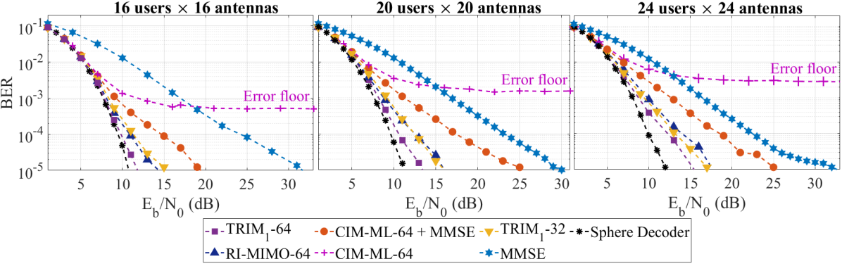
Figure 3: Bit Error Rate (BER) Curves for (Left) 16$\times$16, (Center) 20$\times$20, (Right) 24$\times$24 MIMO and BPSK modulation, illustrating the error floor problem and performance of all the tested solvers. The curves are computed over $\approx$25K MIMO instances (128 channel instances, 198 transmit vectors per channel).

A tree search algorithm for ML-MIMO receiver represents the process of finding the optimal solution by visiting various leaf nodes of a suitably constructed search tree. For an M-QAM constellation, there are M possible symbols for each user. We represent the M possibilities for user-1 by M nodes at depth 1. Each of these nodes has M children, which represent the M possibilities for user 2, and so on. Any path from the root to a leaf node will represent a candidate solution for the ML-MIMO problem. As noted in Section II, there exist several techniques that involve traversing this search tree to obtain good quality solutions in polynomial complexity.

In this section, we build on the ideas of RI-MIMO, to further improve the performance of CIM based ML-MIMO receiver by proposing a hybrid tree search algorithm. The maximum-likelihood MIMO receiver described in Eq. 2 can be expressed using a QR decomposition, $\mathbf{H}=\mathbf{QR}$,

$$\mathbf{\hat{x}_{ML}}=\min_{\mathbf{x}\in\Omega^{N_{t}}}\|\mathbf{w}-\mathbf{R}\mathbf{x}\|^{2},$$ (14)

where $\mathbf{w}=\mathbf{Q}^{\dagger}\mathbf{y}$. If we fix the symbol corresponding to user $N_{t}$ to $u$, then $\mathbf{x}=[\mathbf{v}\text{~{}~{}}u]^{T}$, where $\mathbf{v}\in\Omega^{N_{t}-1}$. Let $\mathbf{R}=\left[\bar{\mathbf{R}}\text{ }\bar{\mathbf{c}}\right]$, where $\mathbf{\bar{R}}$ is an $(N_{t}-1)\times(N_{t}-1)$ upper triangular matrix, $\mathbf{\bar{c}}$ is $(N_{t}-1)\times 1$ and $r$ is a scalar. Substituting this is Eq. 14 and simplifying, we obtain:

$$\mathbf{\hat{v}}_{ML}=\min_{\mathbf{v}\in\Omega^{N_{t}-1}}\|(\mathbf{\bar{w}}-\mathbf{\bar{c}}u)-\mathbf{\bar{R}}\mathbf{v}\|^{2}.$$ (15)

This has the same form as Eq. 2 and can be solved using RI-MIMO techniques. The same procedure can be extended if we fix symbols corresponding to more than one user.

We use this formulation for building a tree search algorithm, TRIM_d-$N_{a}$, augmented by RI-MIMO-$N_{a}$. While solving the ML-MIMO problem, we consider all possibilities for $d$ users, which is the same as considering all nodes in the search tree up to depth ($d$). For each branch of the search tree, once we fix the symbols corresponding to $d$ users, we formulate the maximum likelihood problem for the remaining users as illustrated above, and solve it using RI-MIMO-$N_{a}$, as illustrated in Section V. In the end, we select the best solution out of all the candidate solutions obtained by RI-MIMO-$N_{a}$ sub-problems corresponding to various branches of the search tree. Note that for an $M$-QAM constellation, TRIM_d-$N_{a}$ requires $M^{d}\times N_{a}$ anneals.

VI Evaluation

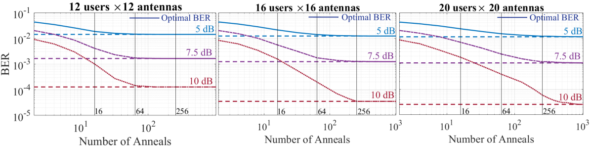
Figure 4: BER vs. $N_{a}$ for (left) $12\times 12$, (center) $16\times 16$ and (right) $20\times 20$ MIMO and BPSK modulation at 5, 7.5 and 10 dB SNR: Illustrating that the BER of RI-MIMO reduces rapidly with increase in number of anneals per instance and asymptotically approaches the optimal BER. The curves are computed over $\approx$25K MIMO instances (128 channel instances, 198 transmit vectors per channel).

In this section, we will perform an extensive evaluation of RI-MIMO and TRIM in various scenarios. We will study the performance of RI-MIMO considering some practical constraints of Ising Machines (IM), like the finite precision available to program the Ising coefficients. We will also evaluate RI-MIMO and TRIM for various modulation schemes, MIMO sizes, and under adaptive MCS (Modulation and Coding Scheme).

We will simulate (using MATLAB, see IV-A) uplink wireless MIMO transmission between $N_{t}$ users with one transmit antenna each and a base station with $N_{r}$ receive antenna. We assume Rayleigh fading channel between them and additive white Gaussian noise (AWGN) at the receiver. We further assume, for simplicity, that the channel is known at the receiver and all users use the same modulation scheme. The BER of an $N_{t}\times N_{r}$ MIMO system is calculated as the mean BER of the $N_{t}$ independent data streams transmitted by $N_{t}$ users.

VI-A BER Performance

For BER plots, let us say the lowest BER we want to plot is $BER_{l}$, then we consider an input bitstream of size several times ($\geq 4\times$) bigger than $\frac{1}{BER_{l}}$ and is equally divided among all the users in the system. We simulate data transmission from users to the base station, assuming a slow Rayleigh fading channel. Each channel instance is generated according to the Rayleigh fading model, and the channel is assumed to remain unchanged over several transmissions. The exact statistics of the experiments are described along with them. We simulate decoding at the BS and compare the decoded bitstream and the input bitstream to compute the BER.

For computing throughput associated with an error correction code with code rate: $c_{r}$, coded BER: $BER_{coded}$ (output of the simulator), number of users: $N_{t}$, data transmission rate per user: $Tr$ and frame size of $L$ bits, we use the following relations:

$$FER=1-(1-BER_{coded})^{L}$$ (16)

$$Tput=N_{t}\times Tr\times(1-FER)$$ (17)

We start comparing the optimal decoder (the Sphere Decoder) and the linear MMSE decoder against RI-MIMO and the unregularized ML-MIMO using as a test case BPSK 16$\times$16. This case will represent a baseline for our benchmarks and their sophistication. Note that a trivial way to remove the error floor is to take the better solution out of those generated by MMSE and CIM-ML-$M_{a}$. We see from Fig 3 that RI-MIMO provides much better BER than CIM-ML, mitigating the error floor problem associated with it. We note that if we run concurrently MMSE and ML-MIMO for each instance and we select the best of both results (CIM-ML+MMSE), we are still less performant than RI-MIMO. TRIM performs similar to RI-MIMO when both algorithms execute the same number of total anneals. (TRIM₁-32 vs RI-MIMO-64). However, as we will see later, this is not the case when higher modulations are used. The best performing algorithm is TRIM₁-64, which achieves near-optimal performance for $16\times 16$ and $20\times 20$ MIMO with BPSK modulation. For $24\times 24$ MIMO, we see that the performance gap between TRIM₁-64 and Sphere Decoder increases, and a higher number of anneals are required to bridge the gap.

VI-B From Simulation to CIM Hardware Implementation

MIMO Order	Modulation	$\mathbf{N_{a}}$	$\mathbf{N_{s}}$	Throughput Requirement
Standard LTE $2\times 2$	16 QAM	16	8	$1.344\times 10^{5}$ anneals per ms
Massive MIMO $16\times 32$	BPSK	16	16	$1.344\times 10^{5}$ anneals per ms
Large MIMO $16\times 16$	BPSK	64	16	$5.376\times 10^{5}$ anneals per ms
Large MIMO $16\times 16$	BPSK	128	16	$1.075\times 10^{6}$ anneals per ms
Large MIMO $20\times 20$	BPSK	64	20	$5.376\times 10^{5}$ anneals per ms
Large MIMO $16\times 16$	4 QAM	128	32	$1.075\times 10^{6}$ anneals per ms
Large MIMO $8\times 8$	16 QAM	256	32	$2.15\times 10^{6}$ anneals per ms
Large MIMO $16\times 16$	16 QAM	256	64	$2.15\times 10^{6}$ anneals per ms

TABLE II: Requirements for an Ising machine (or set of Ising machines) to meet the Ising mapping and LTE processing constraints for various MIMO systems. $N_{\textrm{a}}$ is the number of anneals required per Ising instance to obtain a satisfactorily accurate solution. $N_{\textrm{s}}$ is the number of spins in each Ising instance. In this table we assume that for all MIMO orders listed, 8400 Ising instances need to be solved every 1 millisecond. Throughput Requirement gives the number of anneals (of instances each with $N_{\textrm{s}}$ spins) that the set of Ising machines needs to process in a millisecond, given by $8400\times N_{\textrm{a}}/1~{}\textrm{ms}$.

While this study is performed with a simulator, our objective is to predict the performance and understand the trade-offs for designing a future hardware implementation of a CIM for ML-MIMO. To estimate the feasibility for MIMO decoding, we need to compare the computational requirements versus the perspective capabilities on a real-world perspective machine.

As per the LTE specifications, a typical LTE deployment with 10 MHz bandwidth and 15KHz sub-carrier spacing produces 8400 MIMO detection problems (corresponding to 14 OFDM symbols per sub-frame and 600 sub-carriers) every sub-frame of 1-millisecond duration. It is important to note that every instance is independent, so different instances can be solved in an embarrassingly parallel fashion if there are enough spin variables available in the machine. In figure 4, we look at the variation of BER with the Number of Anneals per instance ($N_{a}$) and try to characterize the value of $N_{a}$ required to provide near-optimal performance. We simulate the RI-MIMO-$N_{a}$ system, with BPSK modulation, for various values of $N_{a}$. In Fig. 4, we illustrate the variation of RI-MIMO BER with $N_{a}$ for $12\times 12$, $16\times 16$ and $20\times 20$ MIMO with BPSK modulation at 5, 7.5, and 10 dB. We see that at first, the RI-MIMO-BER reduces with increasing $N_{a}$ and asymptotically approaches the optimal BER (Sphere Decoder). Based on the evaluation of the BER performance of our proposed algorithms, as discussed in the previous section, we see that we need to study the performance of our proposed methods using a number of anneals of the order of $N_{a}=16-256$ depending on the modulation and size of the MIMO problem.

In Table II we list the regimes of MIMO operation that are compatible with plausibly near-term Ising machines. For each regime, the table gives a throughput requirement that a set of Ising machines would need to satisfy. The fundamental requirement we assume in all the regimes is that 8400 Ising instances must be solved within 1 millisecond. Given our findings from simulations of how many anneals ($N_{\textrm{a}}$) need to be performed to achieve suitable MIMO performance for each regime, we can characterize the requirement for the set of Ising machines in terms of how many anneals they must perform in total within 1 ms. Note that different MIMO regimes require Ising instances with different numbers of spins ($N_{\textrm{s}}$) to be solved—so, for example, building a set of Ising machines capable of meeting the requirements for Large MIMO $8\times 8$ with 16-QAM modulation is different than for Large MIMO $16\times 16$ with 16-QAM modulation because while they both require throughput of $2.15\times 10^{6}$ anneals per ms, the former requires anneals of 32-spin Ising instances and the latter requires anneals of 64-spin Ising instances.

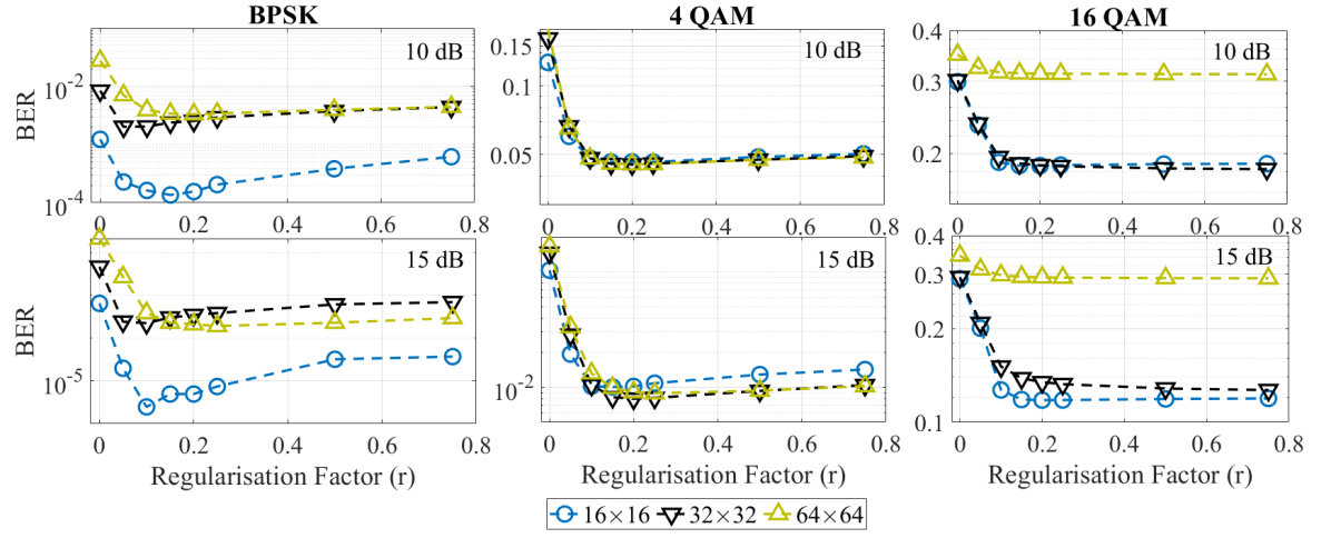
Figure 5: Bit Error Rate at 10 dB and 15 dB SNR , illustrating the performance of RI-MIMO on Coherent based Ising Machines (CIM) for various value of regularisation factor with different MIMO sizes and modulation (using 64 anneals per instance).

The length of a single anneal is defined in Section IV-A and corresponds (in discretized dynamics) to 128 updates of the spin configuration during the anneal. The results in Table II and our discussion so far have not been specific to any particular CIM implementation and will generalize to other forms of Ising machines that have similar working mechanisms [46], including electronic oscillator-based Ising machines [27]. However, we will now briefly give some interpretation of our results that is specific to CIMs, and in particular, time-multiplexed CIMs. In time-multiplexed CIMs such as those reported in Refs. [22, 23, 24, 71], the length of an anneal (128) corresponds to the number of roundtrips of pulses around an optical cavity. In Ref. [71], pulses representing spins are separated in time in a cavity by 200 picoseconds; in a CIM system with such a pulse spacing the time required for a single roundtrip is $N_{\textrm{s}}\times 200~{}\textrm{ps}$, and hence the time required for a single anneal is $128\times N_{\textrm{s}}\times 200~{}\textrm{ps}$. If we consider the MIMO regimes for which Ising instances with $N_{\textrm{s}}=64$ spins need to be solved, a single anneal will take $1.638~{}\mu\textrm{s}$. Therefore the number of 64-spin anneals that a single time-multiplexed CIM with 200-ps pulse spacing can perform per millisecond is $\approx 610$. Table II shows, for example, that the MIMO regime of Large MIMO $16\times 16$ and $16$ QAM requires a throughput of $2.15\times 10^{6}$ anneals per ms. This implies that $(2.15\times 10^{6}/610.4)\approx 3522$ copies of this type of CIM, operating in parallel, would be required to meet the requirements for this MIMO regime. Even if the roundtrip time was decreased by a factor of 20 (which is currently under experimental investigation by groups working on time-multiplexed CIMs), leading to a $20\times$ increase in the speed of a single CIM and hence a $20\times$ reduction in the number of CIMs needed to meet the throughput requirement, one would still need $\approx 176$ copies of the CIM. While it is certainly conceivable that one could construct hundreds or thousands of copies of such a 64-spin time-multiplexed CIM, especially when considering on-chip implementations using integrated photonics [72], it is clear that meeting the throughput requirement is a large practical engineering challenge.

Returning to a discussion applicable to Ising machines generically, it seems likely that any Ising machine—be it a CIM or any other type—will struggle to meet the throughput requirement using just a single machine solving Ising instances serially because to solve 8400 instances in 1 ms serially, one needs to solve (up to the accuracy achieved using $N_{a}$ anneals in a CIM) each instance in 119 ns, and even for Ising instances with only 64 spins, this seems beyond any current machine or approach. Therefore it seems likely that multiple copies of an Ising machine running in parallel will be needed, and the question turns to how many parallel Ising machines are needed and how practical is operating such a set of machines at each LTE base station? This is a major open question and challenge for the Ising-machine community at large.

VI-C Optimal regularisation factor for RI-MIMO and Higher Order Modulations

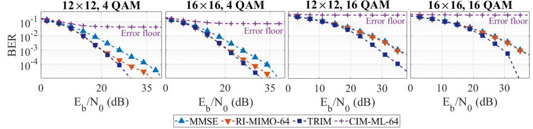
Figure 6: Bit Error Rate Curves higher order modulation schemes, illustrating the performance of RI-MIMO and TRIM on Coherent based Ising Machines (CIM). TRIM executes total 64 anneals for each instance (same as RI-MIMO-64).The curves are computed over $\approx$25K MIMO instances (128 channel instances, 198 transmit vectors per channel).

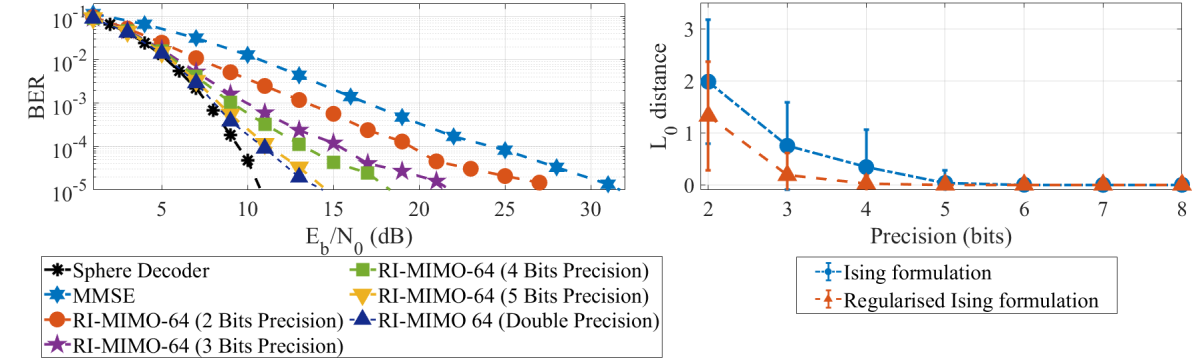
Figure 7: (a) Bit Error Rate Curves for 16x16 MIMO and BPSK modulation, illustrating the performance of RI-MIMO on Coherent based Ising Machines (CIM) with varying precision. The curves are computed over $\approx$50K MIMO instances (256 channel instances, 198 transmit vectors per channel).(b) $L_{0}$ deviation from the ground state for $8\times 8$ MIMO and BPSK modulation.

In this section, we will discuss the tuning of the value for the regularisation prefactor for RI-MIMO in Eq. 10, $r(\rho,M,N_{t})$, relative to the magnitude of Ising coefficients of the original un-regularised problem. To maintain consistency of results, we normalize the Ising coefficients of the original problem to $[-1,1]$. Starting from the $16\times 16$ BPSK baseline MIMO system, we compute performance for various values.

In order to determine the impact of modulation($M$), number of users ($N_{t}$) and SNR ($\rho$) on the optimal value of $r(\rho,M,N_{t})$, we look at BER vs regularisation factor for various MIMO sizes and modulations, while keeping SNR fixed at 10 dB and 15 dB in Fig. 5. We note that the BER reduces dramatically from $r=0$ (unregularized) to around $r=0.1$, beyond which the sensitivity of BER to choice of $r$ is not much. We note that the optimal value is around 0.15, which acts as a threshold: for larger $r$ the BER performance is only slightly affected. Based on these observations, for practicality, in our benchmarks, we will be using $r(\rho,M,N_{t})=0.15$, irrespective of SNR, modulation, and the number of users. In a practical system, similar experiments can be used to construct a lookup table for the optimal value of $r$ as a function of $M,N_{t}$ and $\rho$.

Using the prescriptions above, Fig. 6 provides the BER performance of RI-MIMO and TRIM for a $12\times 12$ and $16\times 16$ MIMO system with 4 QAM and 16 QAM modulations. We see that the error floor problem appears even for higher modulation, and RI-MIMO successfully mitigates it. Note that the difference between RI-MIMO and MMSE reduces as the modulation order increases. However, TRIM provides superior performance for the same number of total anneals and provides 10-15 dB gain over MMSE.

VI-D Finite Precision of Ising Machines

Physical realizations of CIMs typically involve analog control of the couplings between spins. Consequently, the precision in specifying the coefficients of an Ising problem ($J_{ij}$) can be limited. Currently, published results of optical hardware implementations of CIMs have only been for problems where the Ising coefficients take values $\{-1,0,1\}$, and even digital optimized implementations on GPUs are limited to floats encoded with $\approx 5$ bits. While the precision may be improved, any analog machine will have a rather strict practical limit on how much precision can be achieved. Current quantum annealers have a similar limit on specifying Ising coefficients accurately, which can lead to drastic deterioration of performance [73]. In this subsection, we look at the performance of RI-MIMO under the constraint that Ising coefficients can be expressed using $K$ bits only. All Ising coefficients are normalized to $[-1,1]$; one bit is used to indicate the sign (positive/negative), and $K$-1 bits are used to express the decimal part of the Ising coefficient. We simulate RI-MIMO with limited precision CIM for the baseline $16\times 16$ BPSK MIMO system in Fig. 7(a). We see that 5 bits of precision are enough for achieving performance similar to double precision for the given system. If we reduce precision below 5 bits, then the performance starts to deteriorate. It is interesting to note that, even with 2-bit precision, where the Ising coefficients can take values $\{-1,0,1\}$ only, RI-MIMO performs much better than MMSE. Note that for a more complicated system with more users or higher modulations, the precision requirement might be higher - but we leave the analysis to a future study. Independently from the optimization solver, we could study the ”Resilience” [74] of a problem as a metric to study the changes in ground state configuration due to noise in representing Ising coefficients. In Fig. 7(b), we look at the $L_{0}$ distance between the original ground state and the ground state of the Ising problem represented with finite precision. It is a natural metric for wireless applications; as for BPSK, it essentially represents the BER. In Fig. 7(b), we observe for an indicative $8\times 8$ BPSK instance set that $L_{0}$ deviation is nearly zero for 5 bits of precision and that the regularized Ising formulation is more resilient than the unregularized.

VI-E Massive MIMO

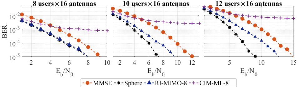
Figure 8: Bit Error Rate Curves for various Massive MIMO system with BPSK modulation and 16 antennas at the base station, illustrating the performance of RI-MIMO. The curves are computed over $\approx$100K MIMO instances (512 channel instances, 198 transmit vectors per channel).

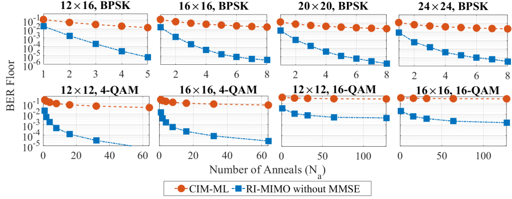
Figure 9: Variation of Error Floor with the number of anneals if RI-MIMO is run without considering MMSE solution as a candidate for various MIMO systems, illustrating that it takes only a few anneals to reduce the resultant error floor to the very low values. In contrast, the error floor associated with CIM-ML reduces very slowly with an increasing number of anneals.

In this section, we will address the need and performance of RI-MIMO/TRIM for massive MIMO systems. Massive MIMO systems tend to have a much higher number of antennas at the receiver than at the transmitter. Due to this, the channel is extremely well-conditioned, and even linear detectors such as MMSE or iterative algorithms can perform extremely well [35]. However, having a large number of antennas at the base station and yet supporting a small number of users reduces the overall cell throughput. Hence, the low BER of linear methods comes at the price of the total number of users served. We will see that for massive MIMO systems, where the linear methods are not optimal, RI-MIMO can be used to obtain optimal performance with very low complexity. In Massive MIMO systems, where the ratio between the number of receiver antennas and the number of transmitter antennas is three or more, MMSE can provide performance similar to the Sphere Decoder. However, the total cell throughput achieved is much lower than what may be possible, with near-optimal MIMO detection, in an equivalent large MIMO system (where the number of receiver antennas and transmitter antennas is the same). In Fig. 8 we look at massive MIMO systems with 16 antennas at the base station and BPSK modulation. We see that for $8\times 16$ and $10\times 16$ MIMO with BPSK, the MMSE decoder is sub-optimal, and RI-MIMO can provide near-optimal performance at very low complexity.

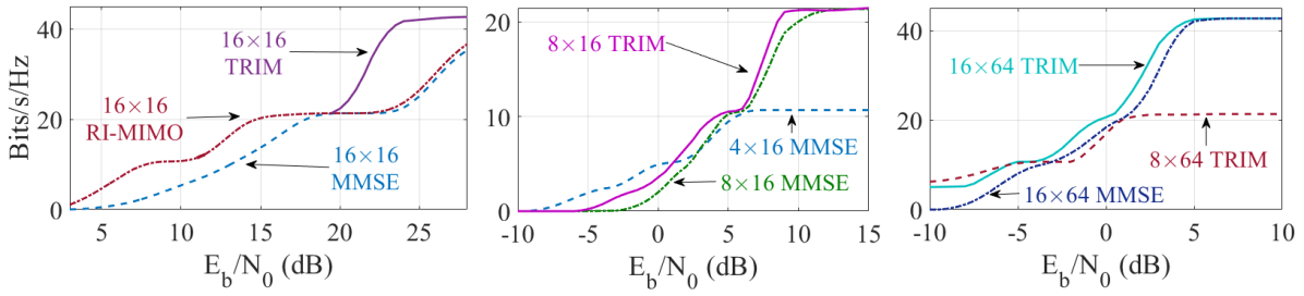
Figure 10: Spectral Efficiency: Comparison between throughput of MMSE, TRIM, RI-MIMO-64 (using adaptive MCS for all) in large/massive MIMO scenarios

Before we go ahead and look at spectral efficiency, note that if we do not consider the MMSE solution as a candidate, then RI-MIMO will have an error floor as well. However, due to a much higher probability of success than the conventional approach, the error floor associated with RI-MIMO will be much lower and reduced much more quickly. We see from Fig. 9 that it take just 4-6 anneals per instance (much less than the conventional approach) for a $16\times 16$, $20\times 20$, and $24\times 24$ MIMO system with BPSK modulation, to reduce the error floor to $10^{-5}$. In contrast, the error floor associated with CIM-ML reduces very slowly, and even with 64 anneals per instance, it remains around $10^{-}3$ (as seen in Fig 3). In Fig. 9, we also observe the same trend for massive MIMO system ($12\times 16$, BPSK), and large MIMO systems ($12\times 12$ and $16\times 16$) with 4-QAM and 16-QAM modulations. Note that, for 16-QAM modulation, even though the error floor for RI-MIMO decreases much faster than the conventional approach, it is still high. This is consistent with our previously observed results that RI-MIMO performance needs to be improved for 16-QAM modulation. If we consider the MMSE solution as a candidate, then there is no error floor, as MMSE will make sure that BER goes to zero as SNR goes to infinity.

VI-F Throughput with MCS adaptation

In this section, we will try to look at the spectral efficiency of RI-MIMO. In a practical system, the Modulation and Coding Scheme (MCS) associated with the data transmission is selected dynamically based on the SNR experienced by the user. Usually, the BS has a list fixed set of (modulation, coding rate) and selects the suitable tuple based on Channel State Information (CSI) measurements. To emulate such a system, we consider several MIMO systems that use feed-forward convolutional coding with 1500-byte packets for data transmission.

Using a higher modulation allows us to transmit more bits per symbol; however, it also reduces the hamming distance between possible symbols and hence increases the probability of error. Similarly, using a lower code rate allows a system to correct more errors but requires transmitting more redundant bits as well. Usually, there is an Adaptive Modulation and Coding (AMC) module that selects a suitable MCS based on the CSI measurements to maximize the throughput performance. For this section, we ignore the complexities of the AMC module and assume that there is an oracle AMC that always selects the best MCS such that the overall throughput is maximized at any given SNR. The AMC module can select among BPSK, 4-QAM, or 16-QAM modulation, and among $\dfrac{1}{3}$, $\dfrac{1}{2}$ or $\dfrac{2}{3}$ convolutional coding rate.

We see from Fig 10(a) that RI-MIMO and TRIM allows us to operate using aggressive modulations and coding schemes and hence achieve much better performance. In particular RI-MIMO achieves around 2.5$\times$ more throughput in low-SNR regime ($\approx 7.5dB$) and 2$\times$ more throughput in mid-SNR regime( $>$ 15dB). In the high-SNR ( $>$ 20dB) both MMSE and RI-MIMO-64 seem to provide similar throughput, because RI-MIMO-64 is not sufficient for 16 QAM modulation (as noted before). However, TRIM allows us to get good performance with 16 QAM and provides a 2$\times$ throughput gain in the high-SNR regime. With Increasing SNR, the channel capacity also increases; hence we would expect the AMC module to use more aggressive modulations in order to achieve the best possible capacity. Consequently, improving the performance of RI-MIMO/TRIM for 16 QAM and higher modulations remains a key challenge for future work.

Further, we simulate several massive MIMO systems in Fig 10(b) and Fig 10(c). Although massive MIMO systems with a high ratio between the number of antennas at the base station and the number of users, like $4\times 16$, can achieve near-optimal performance with just the MMSE receiver, this simplicity comes at the cost of limiting the overall cell throughput. We see from Fig 10(b) and Fig 10(c) that with RI-MIMO/TRIM, BS can expand these systems to support more users concurrently and drastically increase the overall cell throughput. We see from Fig 10(b) that TRIM allows us to expand a $4\times 16$ MIMO system to $8\times 16$ and increase the overall cell throughput by twice. Note that, even though the spectral efficiency of MMSE and TRIM is similar in high-SNR conditions for $8\times 16$ MIMO, it is not feasible to expand a $4\times 16$ MIMO to $8\times 16$ MIMO with just MMSE because, unlike TRIM, the performance of MMSE is terrible in low SNR situations. In very high-SNR conditions, which can occur in nano-cells and highly beam-formed systems, BS can even expand to a $16\times 16$ large MIMO with RI-MIMO/TRIM for a 4$\times$ increase in the overall cell throughput. InFig 10(c), we observes a similar trend is observed for $8\times 64$ and $16\times 64$ MIMO as well.

VII Conclusion

In this paper, we explore the application of Coherent Ising Machines (CIM) for maximum likelihood detection for MIMO detection. We see that previous approaches used by MIMO detectors based on the Ising model suffer from an error floor problem and, unless many repetitions are allowed, does not have a satisfactory Bit Error Rate (BER) performance in practice. We propose a novel Regularized Ising approach and show that it mitigates the error floor problem and is a viable method to be implemented on the hardware implementation of Coherent Ising Machines. We propose two MIMO detection algorithms based on regularised Ising approach (RI-MIMO and TRIM). We demonstrate, using a CIM simulator, that our algorithms can outperform the previous Ising approach and have the potential to achieve near-optimal performance for large MIMO systems. By means of an extensive numerical evaluation, we see that the Regularized Ising approach has an impressive error performance when compared to the state-of-art. We evaluate the system under various settings (different modulations, massive MIMO, adaptive MCS). We show that our methods can expand the overall cell throughput of a massive MIMO system by supporting more users concurrently. While our experiments use a CIM simulator, we have identified the constraints that need to be satisfied by a physical implementation of the CIM to meet the processing requirements of an LTE system.

Our evaluation is based on simulating a simplified CIM model; as a next step, we plan to evaluate our methods on more recent extensions to the CIM (e.g., variants incorporating amplitude-heterogeneity correction [75, 57]) and on an experimental CIM implementation [23, 24, 71].

In conclusion, our results indicate that Coherent Ising Machines (using the proposed Regularized Ising approach) are a promising candidate for providing a superior alternative to the existing MIMO detection approach and achieving near-optimal performance for practical systems with a large number of users and antennas, although performance and engineering aspects need to be substantially improved for practical deployment, especially for high modulations such as 16-QAM. Most of our methods and results are not specific to CIMs and can also be applied to other types of Ising machines, which is another interesting direction for future work.

Appendix A LTE Uplink Transmission

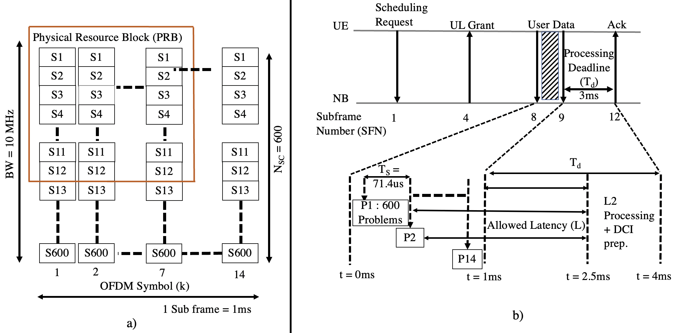
Figure 11: a) LTE UL Frame structure: Illustrating the division of available bandwidth into subcarriers and Physical Resource Blocks (PRBs), which are the basic unit of scheduling. b) LTE UL data transmission: Illustrating the scheduling process and the processing deadline for UL traffic.

Let us discuss how this simplified system model fits into commercial LTE systems. LTE can potentially operate in both TDD (Time Division Duplex) and FDD (Frequency Division Duplex) modes; however, FDD is more commonly used. There are several possible bandwidth (BW) configurations that can be used; an uplink bandwidth of 10MHz is popularly used. LTE uses OFDMA (Orthogonal Frequency Division Multiple Access), and the entire bandwidth is divided in $N_{SC}$ sub-carriers, which have 15KHz sub-carrier spacing. Each sub-carrier can carry a modulated signal independently of others and represents an independent instance of the MIMO problem as described by the above-mentioned system model. For 10MHz BW, as shown in Fig. 11(a), $N_{SC}=600$ which is 9MHz out of the available 10MHz, rest accounts for guard bands. The LTE operation is divided into frames (10ms long) and subframes (1ms long). Each subframe has 14 OFDM symbols and is divided into two slots. The basic unit of scheduling in LTE is called a Physical Resource Block (PRB), which comprises 12 sub-carriers in a slot (7 OFDM symbols). Fig. 11(b) illustrates the UL data transmission procedure; we see that the base station has $T_{d}=3ms$ to process the data received in a subframe before it is required to send an acknowledgment. This processing deadline ($T_{d}$) incorporates both L2 and L1 processing, and we assume that half of it is available for MIMO detection. Each sub-carrier produces one instance of decoding problem, and hence every OFDM symbol will produce at most 600 problems. The allowed latency (L) in solving these problems has to be less than $\frac{T_{d}}{2}$, so the base station can finish the processing in time.

References

- [1] C. Kalalas and J. Alonso-Zarate, “Massive Connectivity in 5G and Beyond: Technical Enablers for the Energy and Automotive Verticals,” in 2020 2nd 6G Wireless Summit (6G SUMMIT), 2020, pp. 1–5.
- [2] S. Narayanan, D. Tsolkas, N. Passas, and L. Merakos, “NB-IoT: A Candidate Technology for Massive IoT in the 5G Era,” in 2018 IEEE 23rd International Workshop on Computer Aided Modeling and Design of Communication Links and Networks (CAMAD), 2018, pp. 1–6.
- [3] Yinan Qi, M. Hunukumbure, M. Nekovee, J. Lorca, and V. Sgardoni, “Quantifying data rate and bandwidth requirements for immersive 5G experience,” in 2016 IEEE International Conference on Communications Workshops (ICC), 2016.
- [4] “IMT Traffic estimates for the years 2020 to 2030,” Tech. Rep. ITU-R Report M.2370-0, July 2015. [Online]. Available: https://www.itu.int/pub/R-REP-M.2370-2015
- [5] J. Oueis and E. Strinati, Uplink Traffic in Future Mobile Networks: Pulling the Alarm, 2016, pp. 583–593.
- [6] B. Trotobas, A. Nafkha, and Y. Louet, A Review to Massive MIMO Detection Algorithms: Theory and Implementation, 2020.
- [7] U. Fincke and M. Pohst, “Improved Methods for Calculating Vectors of Short Length in a Lattice, Including a Complexity Analysis,” Mathematics of Computation, vol. 44, no. 170, pp. 463–471, 1985.
- [8] C. Hung and T. Sang, “A Sphere Decoding Algorithm for MIMO Channels,” in 2006 IEEE International Symposium on Signal Processing and Information Technology, 2006, pp. 502–506.
- [9] D. Tse and P. Viswanath, Fundamentals of Wireless Communication, 2005.
- [10] C. Navarro i Manchon, L. Deneire, P. Mogensen, and T. B. Sorensen, “On the Design of a MIMO-SIC Receiver for LTE Downlink,” in 2008 IEEE 68th Vehicular Technology Conference, 2008, pp. 1–5.
- [11] A. A. Sahrab and I. Marghescu, “Enhanced IRC-SIC algorithm with beamforming for MU-MIMO systems,” in 2015 International Symposium on Signals, Circuits and Systems (ISSCS), 2015, pp. 1–4.
- [12] L. G. Barbero and J. S. Thompson, “Fixing the Complexity of the Sphere Decoder for MIMO Detection,” IEEE Transactions on Wireless Communications, vol. 7, no. 6, pp. 2131–2142, 2008.
- [13] B. Gestner, W. Zhang, X. Ma, and D. V. Anderson, “Lattice Reduction for MIMO Detection: From Theoretical Analysis to Hardware Realization,” IEEE Transactions on Circuits and Systems I: Regular Papers, vol. 58, no. 4, pp. 813–826, 2011.
- [14] E. G. Larsson, O. Edfors, F. Tufvesson, and T. L. Marzetta, “Massive MIMO for next generation wireless systems,” IEEE Communications Magazine, vol. 52, no. 2, pp. 186–195, 2014.
- [15] H. Rahul, S. Kumar, and D. Katabi, “MegaMIMO: Scaling Wireless Capacity with User Demands,” in ACM SIGCOMM 2012, Helsinki, Finland, August 2012.
- [16] X. Gao, Z. Lu, Y. Han, and J. Ning, “Near-optimal signal detection with low complexity based on Gauss-Seidel method for uplink large-scale MIMO systems,” in 2014 IEEE International Symposium on Broadband Multimedia Systems and Broadcasting, 2014, pp. 1–4.
- [17] F. Rusek, D. Persson, B. K. Lau, E. G. Larsson, T. L. Marzetta, O. Edfors, and F. Tufvesson, “Scaling Up MIMO: Opportunities and Challenges with Very Large Arrays,” IEEE Signal Processing Magazine, vol. 30, no. 1, pp. 40–60, 2013.
- [18] M. A. Albreem, M. Juntti, and S. Shahabuddin, “Massive MIMO Detection Techniques: A Survey,” IEEE Communications Surveys Tutorials, vol. 21, no. 4, pp. 3109–3132, 2019.
- [19] D. de Falco and D. Tamascelli, “An introduction to Quantum Annealing,” RAIRO - Theoretical Informatics and Applications, vol. 45, 07 2011.
- [20] A. Finnila, M. Gomez, C. Sebenik, C. Stenson, and J. Doll, “Quantum annealing: A new method for minimizing multidimensional functions,” Chemical Physics Letters, vol. 219, no. 5, pp. 343–348, 1994. [Online]. Available: https://www.sciencedirect.com/science/article/pii/0009261494001170
- [21] Z. Wang, A. Marandi, K. Wen, R. L. Byer, and Y. Yamamoto, “Coherent Ising machine based on degenerate optical parametric oscillators,” Physical Review A, vol. 88, no. 6, p. 063853, 2013.
- [22] A. Marandi, Z. Wang, K. Takata, R. L. Byer, and Y. Yamamoto, “Network of time-multiplexed optical parametric oscillators as a coherent Ising machine,” Nature Photonics, vol. 8, no. 12, pp. 937–942, 2014.
- [23] P. L. McMahon, A. Marandi, Y. Haribara, R. Hamerly, C. Langrock, S. Tamate, T. Inagaki, H. Takesue, S. Utsunomiya, K. Aihara et al., “A fully programmable 100-spin coherent Ising machine with all-to-all connections,” Science, vol. 354, no. 6312, pp. 614–617, 2016.
- [24] T. Inagaki, Y. Haribara, K. Igarashi, T. Sonobe, S. Tamate, T. Honjo, A. Marandi, P. L. McMahon, T. Umeki, K. Enbutsu et al., “A coherent Ising machine for 2000-node optimization problems,” Science, vol. 354, no. 6312, pp. 603–606, 2016.
- [25] Y. Haribara, S. Utsunomiya, and Y. Yamamoto, “Computational Principle and Performance Evaluation of Coherent Ising Machine Based on Degenerate Optical Parametric Oscillator Network,” Entropy, vol. 18, no. 4, 2016. [Online]. Available: https://www.mdpi.com/1099-4300/18/4/151
- [26] F. Böhm, G. Verschaffelt, and G. Van der Sande, “A poor man’s coherent Ising machine based on opto-electronic feedback systems for solving optimization problems,” Nature Communications, vol. 10, p. 3538, 08 2019.
- [27] T. Wang and J. Roychowdhury, “OIM: Oscillator-Based Ising Machines for Solving Combinatorial Optimisation Problems,” in Unconventional Computation and Natural Computation, I. McQuillan and S. Seki, Eds. Cham: Springer International Publishing, 2019, pp. 232–256.
- [28] M. Kim, D. Venturelli, and K. Jamieson, “Leveraging Quantum Annealing for Large MIMO Processing in Centralized Radio Access Networks,” The 31st ACM Special Interest Group on Data Communication (SIGCOMM), 2019.
- [29] M. Kim, S. Mandra, D. Venturelli, and K. Jamieson, “Physics-Inspired Heuristics for Soft MIMO Detection in 5G New Radio and Beyond,” in Proceedings of the 27th Annual International Conference on Mobile Computing and Networking (MobiCom), 2021. [Online]. Available: https://doi.org/10.1145/3447993.3448619
- [30] S. Kasi, P. Warburton, J. Kaewell, and K. Jamieson, “Challenge: A Cost and Power Feasibility Analysis of Quantum Annealing for NextG Cellular Wireless Networks,” arXiv preprint arXiv:2109.01465, 2021.
- [31] K. Sankar, A. Scherer, S. Kako, S. Reifenstein, N. Ghadermarzy, W. B. Krayenhoff, Y. Inui, E. Ng, T. Onodera, P. Ronagh et al., “Benchmark Study of Quantum Algorithms for Combinatorial Optimization: Unitary versus Dissipative,” arXiv preprint arXiv:2105.03528, 2021.
- [32] M. Shafi, A. F. Molisch, P. J. Smith, T. Haustein, P. Zhu, P. De Silva, F. Tufvesson, A. Benjebbour, and G. Wunder, “5G: A Tutorial Overview of Standards, Trials, Challenges, Deployment, and Practice,” IEEE Journal on Selected Areas in Communications, vol. 35, no. 6, pp. 1201–1221, 2017.
- [33] D. Xu, A. Zhou, X. Zhang, G. Wang, X. Liu, C. An, Y. Shi, L. Liu, and H. Ma, “Understanding Operational 5G: A First Measurement Study on Its Coverage, Performance and Energy Consumption,” in Proceedings of the Annual Conference of the ACM Special Interest Group on Data Communication on the Applications, Technologies, Architectures, and Protocols for Computer Communication, ser. SIGCOMM ’20. New York, NY, USA: Association for Computing Machinery, 2020, p. 479–494. [Online]. Available: https://doi.org/10.1145/3387514.3405882
- [34] B. Hassibi and H. Vikalo, “On the sphere-decoding algorithm I. Expected complexity,” IEEE Transactions on Signal Processing, vol. 53, no. 8, pp. 2806–2818, 2005.
- [35] M. Mandloi and V. Bhatia, “Low-Complexity Near-Optimal Iterative Sequential Detection for Uplink Massive MIMO Systems,” IEEE Communications Letters, vol. 21, no. 3, pp. 568–571, 2017.
- [36] Y. Lee, “Low-Complexity MIMO Detection: A Mixture of Basic Techniques for Near-Optimal Error Rate,” IEEE Transactions on Circuits and Systems II: Express Briefs, vol. 63, no. 10, pp. 949–953, 2016.
- [37] R. Qian, T. Peng, Y. Qi, and W. Wang, “Block-Wise MIMO Detection with Near-Optimal Performance and Low Complexity,” in 2010 International Conference on Communications and Mobile Computing, vol. 2, 2010, pp. 356–360.
- [38] M. Chaudhary, N. K. Meena, and R. S. Kshetrimayum, “Local search based near optimal low complexity detection for large MIMO System,” in 2016 IEEE International Conference on Advanced Networks and Telecommunications Systems (ANTS), 2016, pp. 1–5.
- [39] D. Wübben, D. Seethaler, J. Jalden, and G. Matz, “Lattice Reduction,” Signal Processing Magazine, IEEE, vol. 28, pp. 70 – 91, 06 2011.
- [40] S. V. and A. K., “A signal power adaptive regularized sphere decoding algorithm based multiuser detection technique for underdetermined OFDM/SDMA uplink system,” International Journal of Communication Systems, vol. 32, 11 2018.
- [41] I. Kanaras, A. Chorti, M. R. D. Rodrigues, and I. Darwazeh, “A combined MMSE-ML detection for a spectrally efficient non orthogonal FDM signal,” in 2008 5th International Conference on Broadband Communications, Networks and Systems, 2008, pp. 421–425.
- [42] M. Albreem and M. F. Mohd Salleh, “Regularized Lattice Sphere Decoding for Block Data Transmission Systems,” Wireless Personal Communications, 01 2015.
- [43] M. Alghoniemy, “Regularized MIMO decoders,” Journal of Communications Software and Systems, vol. 5, pp. 149–153, 12 2010.
- [44] J. Pan, W.-K. Ma, and J. Jaldén, “MIMO Detection by Lagrangian Dual Maximum-Likelihood Relaxation: Reinterpreting Regularized Lattice Decoding,” IEEE Transactions on Signal Processing, vol. 62, no. 2, pp. 511–524, 2014.
- [45] J. Kukačka, V. Golkov, and D. Cremers, “Regularization for deep learning: A taxonomy,” 10 2017.
- [46] S. K. Vadlamani, T. P. Xiao, and E. Yablonovitch, “Physics successfully implements Lagrange multiplier optimization,” Proceedings of the National Academy of Sciences, vol. 117, no. 43, pp. 26 639–26 650, 2020.
- [47] M. Kim, D. Venturelli, and K. Jamieson, “Leveraging Quantum Annealing for large MIMO processing in centralized radio access networks,” in Proceedings of the ACM Special Interest Group on Data Communication, 2019, pp. 241–255.
- [48] P. Hauke, H. G. Katzgraber, W. Lechner, H. Nishimori, and W. D. Oliver, “Perspectives of quantum annealing: Methods and implementations,” Reports on Progress in Physics, vol. 83, no. 5, p. 054401, 2020.
- [49] C. Roques-Carmes, Y. Shen, C. Zanoci, M. Prabhu, F. Atieh, L. Jing, T. Dubček, C. Mao, M. R. Johnson, V. Čeperić et al., “Heuristic recurrent algorithms for photonic Ising machines,” Nature communications, vol. 11, no. 1, pp. 1–8, 2020.
- [50] M. Prabhu, C. Roques-Carmes, Y. Shen, N. Harris, L. Jing, J. Carolan, R. Hamerly, T. Baehr-Jones, M. Hochberg, V. Čeperić et al., “Accelerating recurrent Ising machines in photonic integrated circuits,” Optica, vol. 7, no. 5, pp. 551–558, 2020.
- [51] M. Babaeian, D. T. Nguyen, V. Demir, M. Akbulut, P.-A. Blanche, Y. Kaneda, S. Guha, M. A. Neifeld, and N. Peyghambarian, “A single shot coherent Ising machine based on a network of injection-locked multicore fiber lasers,” Nature communications, vol. 10, no. 1, pp. 1–11, 2019.
- [52] D. Pierangeli, G. Marcucci, and C. Conti, “Large-scale photonic Ising machine by spatial light modulation,” Physical review letters, vol. 122, no. 21, p. 213902, 2019.
- [53] M. Yamaoka, C. Yoshimura, M. Hayashi, T. Okuyama, H. Aoki, and H. Mizuno, “A 20k-spin Ising chip to solve combinatorial optimization problems with CMOS annealing,” IEEE Journal of Solid-State Circuits, vol. 51, no. 1, pp. 303–309, 2015.
- [54] M. Aramon, G. Rosenberg, E. Valiante, T. Miyazawa, H. Tamura, and H. G. Katzgraber, “Physics-inspired optimization for quadratic unconstrained problems using a digital annealer,” Frontiers in Physics, vol. 7, p. 48, 2019.
- [55] H. Goto, K. Tatsumura, and A. R. Dixon, “Combinatorial optimization by simulating adiabatic bifurcations in nonlinear Hamiltonian systems,” Science Advances, vol. 5, no. 4, p. eaav2372, 2019.
- [56] H. Goto, K. Endo, M. Suzuki, Y. Sakai, T. Kanao, Y. Hamakawa, R. Hidaka, M. Yamasaki, and K. Tatsumura, “High-performance combinatorial optimization based on classical mechanics,” Science Advances, vol. 7, no. 6, p. eabe7953, 2021.
- [57] T. Leleu, F. Khoyratee, T. Levi, R. Hamerly, T. Kohno, and K. Aihara, “Chaotic Amplitude Control for Neuromorphic Ising Machine in Silico,” arXiv preprint arXiv:2009.04084, 2020.
- [58] K. Tatsumura, M. Yamasaki, and H. Goto, “Scaling out Ising machines using a multi-chip architecture for simulated bifurcation,” Nature Electronics, vol. 4, no. 3, pp. 208–217, 2021.
- [59] B. Sutton, K. Y. Camsari, B. Behin-Aein, and S. Datta, “Intrinsic optimization using stochastic nanomagnets,” Scientific reports, vol. 7, no. 1, pp. 1–9, 2017.
- [60] J. Grollier, D. Querlioz, K. Camsari, K. Everschor-Sitte, S. Fukami, and M. D. Stiles, “Neuromorphic spintronics,” Nature electronics, vol. 3, no. 7, pp. 360–370, 2020.
- [61] F. Cai, S. Kumar, T. Van Vaerenbergh, X. Sheng, R. Liu, C. Li, Z. Liu, M. Foltin, S. Yu, Q. Xia et al., “Power-efficient combinatorial optimization using intrinsic noise in memristor Hopfield neural networks,” Nature Electronics, vol. 3, no. 7, pp. 409–418, 2020.
- [62] M. Kim, S. Kasi, P. A. Lott, D. Venturelli, J. Kawell, and K. Jamieson, “Heuristic Quantum Optimization for 6G Wireless Communications,” IEEE Network (to appear), vol. 35, no. 4, 2021.
- [63] Towards Hybrid Classical-Quantum Computation Structures in Wirelessly-Networked Systems, 2020.
- [64] S. Kasi, A. K. Singh, D. Venturelli, and K. Jamieson, “Quantum Annealing for Large MIMO Downlink Vector Perturbation Precoding,” in Forthcoming, IEEE International Conference on Communications (ICC), 2021.
- [65] K. P. S. e. a. Jaijeet Roychowdhury, Joachim Wabnig, “Performance of Oscillator Ising Machines on Realistic MU-MIMO Decoding Problems, 22 September 2021, PREPRINT (Version 1).”
- [66] H. Vikalo and B. Hassibi, “On the sphere-decoding algorithm II. Generalizations, second-order statistics, and applications to communications,” IEEE Transactions on Signal Processing, vol. 53, no. 8, pp. 2819–2834, 2005.
- [67] X. Lu, X. Yang, S. Jin, C. Wen, and W. Lu, “TDD-based massive MIMO system with multi-antenna user equipments,” in 2017 23rd Asia-Pacific Conference on Communications (APCC), 2017, pp. 1–6.
- [68] A. Lucas, “Ising formulations of many NP problems,” Frontiers in Physics, vol. 2, p. 5, 02 2014.
- [69] Z. Bian, F. A. Chudak, W. Macready, and G. Rose, “The Ising model : teaching an old problem new tricks,” 2010.
- [70] A. Cho, “Odd Computer Zips Through Knotty Tasks,” Science (New York, NY), vol. 354, no. 6310, pp. 269–270, 2016.
- [71] T. Honjo, T. Sonobe, K. Inaba, T. Inagaki, T. Ikuta, Y. Yamada, T. Kazama, K. Enbutsu, T. Umeki, R. Kasahara, K. ichi Kawarabayashi, and H. Takesue, “100,000-spin coherent Ising machine,” Science Advances, vol. 7, no. 40, p. eabh0952, 2021.
- [72] K. Luke, P. Kharel, C. Reimer, L. He, M. Loncar, and M. Zhang, “Wafer-scale low-loss lithium niobate photonic integrated circuits,” Optics Express, vol. 28, no. 17, pp. 24 452–24 458, 2020.
- [73] A. Pearson, A. Mishra, I. Hen, and D. Lidar, “Analog errors in quantum annealing: doom and hope,” npj Quantum Information, vol. 5, p. 107, 11 2019.
- [74] Z. Zhu, A. Ochoa, S. Schnabel, F. Hamze, and H. Katzgraber, “Best-case performance of quantum annealers on native spin-glass benchmarks: How chaos can affect success probabilities,” Physical Review A, vol. 93, 05 2015.
- [75] T. Leleu, Y. Yamamoto, P. L. McMahon, and K. Aihara, “Destabilization of local minima in analog spin systems by correction of amplitude heterogeneity,” Physical review letters, vol. 122, no. 4, p. 040607, 2019.