Quantum-Electrodynamical Time-Dependent Density Functional Theory. I. A Gaussian Atomic Basis Implementation

Abstract

Inspired by the formulation of quantum-electrodynamical time-dependent density functional theory (QED-TDDFT) by Rubio and coworkers, we propose an implementation that uses dimensionless amplitudes for describing the photonic contributions to QED-TDDFT electron-photon eigenstates. The leads to a symmetric QED-TDDFT coupling matrix, which is expected to facilitate the future development of analytic derivatives. Through a Gaussian atomic basis implementation of the QED-TDDFT method, we examined the effect of dipole self-energy, rotating wave approximation, and the Tamm-Dancoff approximation on the QED-TDDFT eigenstates of model compounds (ethene, formaldehyde, and benzaldehyde) in an optical cavity. We highlight, in the strong coupling regime, the role of higher-energy and off-resonance excited states with large transition dipole moments in the direction of the photonic field, which are automatically accounted for in our QED-TDDFT calculations and might substantially affect the energy and composition of polaritons associated with lower-energy electronic states.

I Introduction

Quantum optics effects on atoms have been extensively studied during the last several decades,[1, 2, 3, 4, 5, 6, 7, 8, 9] enabling scientists to shift atomic energy levels,[10, 11] tune atomic electronic transition rates,[12, 13, 14] and generate quantum systems with atom-atom entangled states.[15, 16] In contrast, the behavior of molecules in optical cavities attracted a lot of attention only in recent years.[17, 18, 19, 20, 21, 22, 23] In particular, several molecules have been shown to couple strongly to a quantized radiation field, causing their electronic states to hybridize with the cavity photon levels to produce superpositions and entanglements.[2, 24, 25] The study of such entangled states lead to the establishment of the field of polariton chemistry, which focuses on the use of optical cavities to manipulate chemical and photochemical reactivities,[26, 27, 28, 29, 30, 31, 32, 33, 34, 35, 36, 37, 38, 39, 39, 23] modify the intersystem crossing rates,[27, 28, 37, 40, 41, 39] and enhance organic molecule light emitting efficiencies.[42, 43, 44, 45, 46, 47, 48, 49, 50]

In principle, a coupled molecule-photon system is best described by the relativistic quantum field theory (QFT).[51] But to avoid the computational complexity of QFT, many non-relativistic and simplified theories have been developed.[52] Within the Rabi model, for instance, one adopts a semiclassical approach that combines a non-relativistic quantum mechanical description for the molecule and a classical description of the electromagnetic field.[53, 54, 55, 56] The Pauli-Fierz model was introduced to provide a consistent treatment of the spontaneous emission.[57, 58] Jaynes and Cummings proposed two other similar quantum models, which are known as the Jaynes-Cummings (JC) model and rotating-wave approximation (RWA).[59, 60] Within both models, the counter-rotating terms (CRT) are neglected, which turns out to be a valid approximation for the resonance and near-resonance conditions and weak coupling regimes.[59, 60, 52]

In the study of polariton chemistry, it has been common to restrict the description of each electronic system to simplified two- or three-state model.[55, 61, 56, 62, 63, 64, 65, 66, 67, 23, 68] The corresponding input parameters (energy levels and coupling elements), on which the models would heavily rely, are obtained from either experiments or first-principles quantum chemistry calculations. Through employing these models, it has been predicted that the coupling of molecular systems to quantized radiation modes could substantially modify the potential energy surfaces and create new conical intersections,[27, 28, 69, 40] suppress or enhance photoisomerization reactions,[70, 71, 72, 47, 73, 74] increase the charge transfer and excitation energy transfer rates,[75, 76, 77, 78, 79, 52] accelerate the singlet fission kinetics,[80, 41] and even control the chemical reactions remotely.[81, 37] These observations open up opportunities to use optical cavities to manipulate chemical and photochemical reactions.

Recently, ab initio quantum mechanical frameworks were proposed to describe interacting electrons and photons.[51, 82, 83, 84, 85, 86, 87, 88, 89, 63, 90, 91, 92, 93] Specifically, Rubio and others developed quantum electrodynamical density functional theory (QEDFT)[82, 83, 84, 86, 94, 89, 95, 96, 93] and quantum electrodynamics coupled-cluster (QED-CC) theory,[97, 98, 99] which inherit an accurate description of molecular electronic structure from time-dependent density functional theory (TDDFT), coupled-cluster theory (CC), equation-of-motion coupled-cluster theory (EOM-CC), and other ab initio electronic structure theories.

In this work, we closely follow the QEDFT method from Rubio and coworkers.[82, 83, 84, 86, 94, 89, 95, 96, 91, 93] Through a slightly modified matrix formulation of linear-response quantum electrodynamical time-dependent density functional theory (QED-TDDFT), we obtain a symmetric TDDFT-Pauli-Fierz (TDDFT-PF) Hamiltonian for coupling molecules and cavity photons. This allows us to systematically examine the effects of CRT, dipole self-energy (DSE), and the Tamm-Dancoff approximation (TDA), and to compare the polariton energies to different model Hamiltonian results. We expect that, as the electron-photon coupling strength increases, there might be (a) a substantial deviation from symmetric Rabi splitting (which arises from the 2-state model Hamiltonian) and (b) significant differences in the polariton energy and compositions among various theoretical models.

This article is organized as follows. The TDDFT-PF formula is derived in Section II.2 and in Appendix A and B (with linear-response and equation-of-motion formulations, respectively), with its no-DSE, RWA, and TDA variations presented in Section II.3. Section III describes our Gaussian atomic basis implementation within the PySCF software package.[100] Preliminary results on the polariton states of ethene, formaldehyde, and benzaldehyde molecules in the optical cavity are reported in Section IV, which is followed by concluding remarks in Section V.

II Theory

II.1 Notation

For a molecule, we will use indices $i,j$ to represent its occupied Kohn-Sham orbitals, and $a,b$ to denote its unoccupied (virtual) Kohn-Sham orbitals. The corresponding orbital energies will be written as $\varepsilon_{i},\varepsilon_{j},\varepsilon_{a}$, and $\varepsilon_{b}$. The dipole moment vector in the basis of these orbitals is

$$\bm{\mu}_{ai}=\bigg{(}\left<a\middle|\hat{x}\middle|i\right>,\left<a\middle|\hat{y}\middle|i\right>,\left<a\middle|\hat{z}\middle|i\right>\bigg{)}$$ (1)

$\mathbf{A}$ and $\mathbf{B}$ refer to conventional TDDFT coupling super-matrices, while $\mathbf{X}$ and $\mathbf{Y}$ are TDDFT amplitudes.[101, 102, 103, 104, 105, 106, 107, 108]

For an optical cavity with $M$ photon modes, its $\alpha$-th mode of frequency is denoted by $\omega_{\alpha}$. The corresponding fundamental coupling strength [63, 91]

$$\bm{\lambda}_{\alpha}=\sqrt{\frac{1}{\epsilon_{0}}}S_{\alpha}(\bm{r}_{0})\bm{\epsilon}_{\alpha},\quad\quad\alpha=1,2,\cdots,M$$ (2)

depends on the transversal polarization vector $\bm{\epsilon}_{\alpha}$. For a Fabry-Pérot cavity of volume $V_{\textrm{tot}}=L_{x}L_{y}L_{z}$ and with mirror planes perpendicular to the $z$-axis, the dimensionless mode function

$$S_{\alpha}(\bm{r})=\sqrt{\frac{2}{V_{\textrm{tot}}}}\textrm{sin}\left(\frac{\alpha\pi z}{L_{z}}\right)$$ (3)

is evaluated at a chosen reference point $\bm{r}_{0}$ for the molecular subsystem. When there are $N$ identical and non-interacting molecules with the same orientation, the effective volume of each molecule, $V_{\mathrm{eff}}=\frac{V_{\textrm{tot}}}{N}$, can be used in place of $V_{\textrm{tot}}$ in Eq. 3.[27]

For each photon mode, the corresponding displacement coordinate and conjugate moment refer to

$$\hat{q}_{\alpha} = \sqrt{\frac{\hbar}{2\omega_{\alpha}}}\left(\hat{b}_{\alpha}+\hat{b}_{\alpha}^{\dagger}\right)$$ (4)

$$\hat{p}_{\alpha} = -i\sqrt{\frac{\hbar\omega_{\alpha}}{2}}\left(\hat{b}_{\alpha}-\hat{b}_{\alpha}^{\dagger}\right)$$ (5)

with $\hat{b}_{\alpha}^{\dagger}$ and $\hat{b}_{\alpha}$ being the creation and annihilation operators for the mode. For convenience, the dot product of the dipole moment of each virtual-occupied pair and the photon field will be written as

$$\lambda_{ai}^{\alpha}=\bm{\mu}_{ai}\cdot\bm{\lambda}_{\alpha}$$ (6)

II.2 QED-TDDFT Equation within the Pauli-Fierz Hamiltonian

For a molecule confined in this optical cavity, by making the Born-Oppenheimer approximation and the long-wavelength or dipole approximation in the length-gauge, its Pauli-Fierz Hamiltonian can be written as[91, 52]

$$\hat{H} = \hat{H}_{\mathrm{elec}}+\sum_{\alpha=1}^{M}\left[\frac{1}{2}\hat{p}_{\alpha}^{2}+\frac{1}{2}\omega_{\alpha}^{2}\left(\hat{q}_{\alpha}-\frac{1}{\omega_{\alpha}}\bm{\lambda}_{\alpha}\cdot\left<\hat{\bm{\mu}}\right>\right)^{2}\right]$$ (7)

$$+\sum_{\alpha=1}^{M}\frac{j_{\alpha}(t)}{\omega_{\alpha}}\hat{q}_{\alpha}$$

where the photon modes interact with the molecular dipole moment, $\left<\hat{\bm{\mu}}\right>$, and $j_{\alpha}(t)$ is the source of the $\alpha$-th cavity mode.

If the electronic Hamiltonian, $\hat{H}_{\mathrm{elec}}$, is described by the Kohn-Sham density functional theory, the corresponding TDDFT-PF equation is shown in the Appendix A and Appendix B to be,

$$\begin{bmatrix}\mathbf{A}+\bm{\Delta}&\mathbf{B}+\bm{\Delta}&\hbar\mathbf{g}^{\dagger}&\hbar\tilde{\mathbf{g}}^{\dagger}\\ \mathbf{B}+\bm{\Delta}&\mathbf{A}+\bm{\Delta}&\hbar\mathbf{g}^{\dagger}&\hbar\tilde{\mathbf{g}}^{\dagger}\\ \hbar\mathbf{g}&\hbar\mathbf{g}&\hbar\bm{\omega}&0\\ \hbar\tilde{\mathbf{g}}&\hbar\tilde{\mathbf{g}}&0&\hbar\bm{\omega}\end{bmatrix}\begin{bmatrix}\mathbf{X}\\ \mathbf{Y}\\ \mathbf{M}\\ \mathbf{N}\end{bmatrix}$$

$$\quad\quad\quad\quad=\hbar\Omega^{\textrm{TDDFT-PF}}\begin{bmatrix}\mathbf{1}&0&0&0\\ 0&-\mathbf{1}&0&0\\ 0&0&\mathbf{1}&0\\ 0&0&0&-\mathbf{1}\end{bmatrix}\begin{bmatrix}\mathbf{X}\\ \mathbf{Y}\\ \mathbf{M}\\ \mathbf{N}\end{bmatrix}$$ (8)

Here, the electron-electron block contains TDDFT supermatices, $\mathbf{A}$ and $\mathbf{B}$, as augmented by the DSE terms,[52, 99]

$$\Delta_{ai,bj}=\sum_{\alpha=1}^{M}\lambda_{ai}^{\alpha}\lambda_{bj}^{\alpha}$$ (9)

while the electron-photon and photon-electron blocks are

$$\hbar g_{bj}^{\alpha}=\hbar\tilde{g}_{bj}^{\alpha}=\sqrt{\frac{\hbar\omega_{\alpha}}{2}}\lambda_{bj}^{\alpha}$$ (10)

whereas the photon-photon block is a diagonal matrix,

$$\omega_{\alpha\beta}=\delta_{\alpha\beta}\omega_{\alpha}$$ (11)

Due to the couplings (i.e., the electron-photon and photon-electron blocks), the $I$-th eigenvector of the TDDFT-PF equation, $(\mathbf{X}^{I},\mathbf{Y}^{I},\mathbf{M}^{I},\mathbf{N}^{I})^{\mathrm{T}}$, contains photonic amplitudes ($\mathbf{M}^{I}$ and $\mathbf{N}^{I}$) in addition to normal electronic amplitudes ($\mathbf{X}^{I}$ and $\mathbf{Y}^{I}$). The ortho–normalization condition is,

$$\sum_{ai}\left(X_{ai}^{I}X_{ai}^{J}-Y_{ai}^{I}Y_{ai}^{J}\right)+\sum_{\alpha}\left(M_{\alpha}^{I}M_{\alpha}^{J}-N_{\alpha}^{I}N_{\alpha}^{J}\right)=\delta_{IJ}$$ (12)

These components could be explained to be the Fourier coefficients of the time-dependent parameters[109, 110, 111] (also see Appendices A and B).

II.3 A Prism of QED-TDDFT Methods

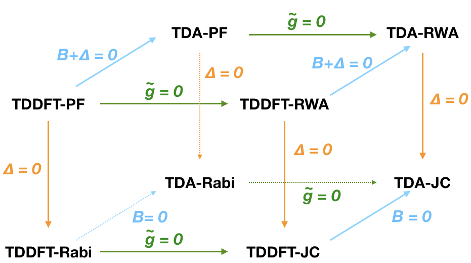
Figure 1: A prism of QED-TDDFT methods.

The TDDFT-PF formula (Eq. 8) can be approximated in a number of ways shown in Fig. 1. First, one can invoke the Tamm-Dancoff approximation (TDA),[103] which sets the $\mathbf{B}+\bm{\Delta}$ elements to zero. One then obtains the TDA-PF model,

$$\begin{bmatrix}\mathbf{A}+\bm{\Delta}&\hbar\mathbf{g}^{\dagger}&\hbar\tilde{\mathbf{g}}^{\dagger}\\ \hbar\mathbf{g}&\hbar\bm{\omega}&0\\ \hbar\tilde{\mathbf{g}}&0&\hbar\bm{\omega}\end{bmatrix}\begin{bmatrix}\mathbf{X}\\ \mathbf{M}\\ \mathbf{N}\end{bmatrix}=\hbar\Omega^{\textrm{TDA-PF}}\begin{bmatrix}\mathbf{1}&0&0\\ 0&\mathbf{1}&0\\ 0&0&-\mathbf{1}\end{bmatrix}\begin{bmatrix}\mathbf{X}\\ \mathbf{M}\\ \mathbf{N}\end{bmatrix}$$ (13)

If the DSE addition, $\bm{\Delta}$, to matrix $\mathbf{A}$ is further removed, one obtains the TDA-Rabi model,[112]

$$\begin{bmatrix}\mathbf{A}&\hbar\mathbf{g}^{\dagger}&\hbar\tilde{\mathbf{g}}^{\dagger}\\ \hbar\mathbf{g}&\hbar\bm{\omega}&0\\ \hbar\tilde{\mathbf{g}}&0&\hbar\bm{\omega}\end{bmatrix}\begin{bmatrix}\mathbf{X}\\ \mathbf{M}\\ \mathbf{N}\end{bmatrix}=\hbar\Omega^{\textrm{TDA-Rabi}}\begin{bmatrix}\mathbf{1}&0&0\\ 0&\mathbf{1}&0\\ 0&0&-\mathbf{1}\end{bmatrix}\begin{bmatrix}\mathbf{X}\\ \mathbf{M}\\ \mathbf{N}\end{bmatrix}$$ (14)

If CRT terms (equal to $\hbar\tilde{\mathbf{g}}^{\dagger}$) are neglected from Eq. 13, it amounts to the RWA approximation,[112]

$$\begin{bmatrix}\mathbf{A}+\bm{\Delta}&\hbar\mathbf{g}^{\dagger}\\ \hbar\mathbf{g}&\hbar\bm{\omega}\end{bmatrix}\begin{bmatrix}\mathbf{X}\\ \mathbf{M}\end{bmatrix}=\hbar\Omega^{\textrm{TDA-RWA}}\begin{bmatrix}\mathbf{1}&0\\ 0&\mathbf{1}\end{bmatrix}\begin{bmatrix}\mathbf{X}\\ \mathbf{M}\end{bmatrix}$$ (15)

Finally, if both DSE and CRT terms are neglected in the TDA-PF formula (Eq. 13), one arrives at the TDA-Jaynes-Cummings (TDA-JC) model

$$\begin{bmatrix}\mathbf{A}&\hbar\mathbf{g}^{\dagger}\\ \hbar\mathbf{g}&\hbar\bm{\omega}\end{bmatrix}\begin{bmatrix}\mathbf{X}\\ \mathbf{M}\end{bmatrix}=\hbar\Omega^{\textrm{TDA-JC}}\begin{bmatrix}\mathbf{1}&0\\ 0&\mathbf{1}\end{bmatrix}\begin{bmatrix}\mathbf{X}\\ \mathbf{M}\end{bmatrix}$$ (16)

Clearly, the first-order DSE correction to the energy of the $I$-th TDA-JC polariton is always positive

$$\Omega_{I}^{\textrm{TDA-RWA}}=\Omega_{I}^{\textrm{TDA-JC}}+\sum_{\alpha=1}^{M}\left|\bm{\lambda}_{\alpha}\cdot\bm{\mu}_{I}\right|^{2}+\cdots$$ (17)

with the transition dipole moment of the $I$-th polariton being

$$\bm{\mu}_{I}^{\textrm{TDA-JC}}=\sum_{ai}X_{I,ai}^{\textrm{TDA-JC}}\bm{\mu}_{ai}$$ (18)

In contrast, the leading CRT correction to the TDA-JC energy is second-order and always negative

$$\Omega_{I}^{\textrm{TDA-Rabi}}=\Omega_{I}^{\textrm{TDA-JC}}-\sum_{\alpha=1}^{M}\frac{g_{\alpha,I}^{2}}{\Omega_{I}^{\textrm{TDA-JC}}+\omega_{\alpha}}+\cdots$$ (19)

where

$$g_{\alpha,I}=\sqrt{\frac{\omega_{\alpha}}{2\hbar}}\left(\bm{\lambda}_{\alpha}\cdot\bm{\mu}_{I}^{\textrm{TDA-JC}}\right)$$ (20)

is the coupling between the $I$-th excited state and the $\alpha$-th cavity mode. Note that under the resonance condition ($\Omega_{I}^{\textrm{TDA-JC}}=\omega_{\alpha}$) as well as $g_{\alpha,I}/\omega_{\alpha}\ll 1$, the leading CRT contributions are second-order to $g_{\alpha,I}$ (and thus $\lambda_{\alpha}$). In those cases, the CRT contribution is roughly $\frac{1}{4}$ of the DSE term, but with an opposite sign. This is different from the report from Huo and coworkers [113, 52] who found the CRT contribution to be $-\frac{1}{2}$ times the DSE term. This discrepancy will be explained later in the context of QED-TDDFT results on test molecules.

As shown in Fig. 1, the TDDFT-Rabi, TDDFT-RWA, and TDDFT-JC models can be defined in a similar procedure starting from the TDDFT-PF model. For instance, the TDDFT-JC working equation would be

$$\begin{bmatrix}\mathbf{A}&\mathbf{B}&\hbar\mathbf{g}^{\dagger}\\ \mathbf{B}&\mathbf{A}&\hbar\mathbf{g}^{\dagger}\\ \hbar\mathbf{g}&\hbar\mathbf{g}&\hbar\bm{\omega}\end{bmatrix}\begin{bmatrix}\mathbf{X}\\ \mathbf{Y}\\ \mathbf{M}\end{bmatrix}=\hbar\Omega^{\textrm{TDDFT-JC}}\begin{bmatrix}\mathbf{1}&0&0\\ 0&\mathbf{-1}&0\\ 0&0&\mathbf{1}\end{bmatrix}\begin{bmatrix}\mathbf{X}\\ \mathbf{Y}\\ \mathbf{M}\end{bmatrix}$$ (21)

Clearly, if this equation (or its TDA-JC counterpart in Eq. 16) is recast in the representation of gas-phase TDDFT (or TDA) eigenstates, it is naturally reduced to the familiar Jaynes-Cummings model, but coupling all excited states to the photon field.

III Computational Details

The QED-TDDFT methods are implemented in a modified version of the PySCF software package[100] as well as the Q-Chem software package.[114] Several functionals (such as PBE,[115] PBE0,[116] B3LYP,[117, 118, 119] and $\omega$B97X-D[120]) are supported in our implementation. Only PBE0 results are presented in the next section, while the use of other functionals is found to lead to qualitatively similar results for the test systems. The lowest eigenstates are solved using Davidson’s diagonalization algorithm.[121]

The ground-state geometries of all the molecules are obtained at the PBE0/6-311++G** level of theory using the Q-Chem software package. Planar Fabry-Pérot micro-cavities are chosen with a frequency resonant (or near-resonant) with the first excited states with a significant oscillation strength of each molecule. Namely, a single fundamental coupling strength vector ($\bm{\lambda}$) is set to be parallel to the transition dipole moment of that particular excited state. The coupling strength is tuned by varying the concentration, while the maximum coupling strength is obtained using the estimated volume of each molecule. Note that this assumes all molecules have exactly the same orientation in the optical cavity. The coupling strengths $\lambda$ are represented in atomic unit, as $1\,\mathrm{au}=1\sqrt{m}_{\mathrm{e}}E_{\mathrm{h}}/e\hbar$.

Furthermore, we consider only one mode of the radiation field with $\alpha$=1 and apply the long wavelength approximation by setting $z$ to half way between the two mirrors. In the end, $S_{\alpha}(\bm{r})$ in Eq. 3 has a value of $\sqrt{\frac{2}{V_{\textrm{eff}}}}$ in all our calculations.

Three molecular systems are considered in this work:

• For the ethene molecule, the effective molecular volume is estimated to be $2331\,a_{0}^{3}$, which corresponds to a maximum coupling strength of $\lambda_{\mathrm{max}}=0.1038\,\mathrm{au}$. The cavity frequency is set to be $6.961$ eV, which is resonant with the first TDA excited state in vacuum; and the coupling strength vector ($\bm{\lambda}$) is parallel to the corresponding electronic transition dipole moment.

• For the formaldehyde molecule, the effective molecular volume is estimated to be $1991\,a_{0}^{3}$, which amounts to a maximum coupling strength of $\lambda_{\mathrm{max}}=0.1123$ au. The cavity frequency is set to be $6.777$ eV in the TDDFT calculations and $6.784$ eV in the TDA calculations, which is in resonant with the second excited state from corresponding gas–phase calculations.

• For the benzaldehyde molecule, the effective molecular volume is estimated to be $73050\,a_{0}^{3}$, with the corresponding maximum coupling strength being $\lambda_{\mathrm{max}}=0.0185\,\mathrm{au}$. The cavity frequency is set to be either in resonance ($4.879\,\mathrm{eV}$ for TDA while $4.810\,\mathrm{eV}$ for TDDFT) with or $0.02\,\mathrm{eV}$ off-resonant ($4.899\,\mathrm{eV}$ for TDA and $4.830\,\mathrm{eV}$ for TDDFT) from the second excitation energy.

IV Results and Discussions

In this section, some preliminary results are presented. In Subsection IV.1, the ethene molecule (C₂H₄) is used as a model system in resonance with the cavity mode to show the equivalence of Jaynes-Cummings model and the corresponding TDA-JC method. In Subsection IV.2, polariton spectra of the formaldehyde molecule (also in resonance with the photon field) are shown at various levels of QED-TDDFT models to systematically analyze the effects of DSE and CRT terms as well as the TDA approximation. In Subsection IV.3, the benzaldehyde molecule is studied as a more practical example of photochrome. The TDA-JC results are compared to those based on the two–state model, where the cavity frequencies are set to be in resonance or off-resonance with the first TDA excitation energy.

IV.1 Ethene

Figure 2: (a) Polariton spectrum of the ethene molecule and (b) photon contribution to each polariton state within the TDA-JC model using PBE0 functional and 6-311++G** basis set, as a function of the coupling strength $\lambda$. Solutions to model Hamiltonians with two or three states are also presented for a comparison.

For the ethene molecule, the first excited state in the gas-phase has an TDA excitation energy of $6.961\,\mathrm{eV}$ and a transition dipole moment in the $x$–direction. As shown in Fig. 2a, this state exhibits an expected Rabi splitting into two polariton states upon the application of a resonant radiation field in the $x$–direction. Within the TDA-JC model, the lower polariton, $\left|P_{1-}\right\rangle$, keeps reducing its energy while the upper polariton, $\left|P_{1+}\right\rangle$, is subjected to a monotonic increase in its energy. The Rabi splitting is clearly becoming non-symmetric. By the maximum coupling strength, $\lambda=0.1038\,\mathrm{au}$, the lower polariton has a TDA-JC excitation energy of $5.965\,\mathrm{eV}$, which translated to a net reduction of $0.996\,\mathrm{eV}$ from its gas-phase value. In contrast, the upper polariton is predicted to have an TDA-JC excitation energy value of $7.270\,\mathrm{eV}$ at $\lambda=0.1038\,\mathrm{au}$, which amounts to a net gain of only $0.308\,\mathrm{eV}$.

A symmetric Rabi splitting of the upper and lower polaritons would be expected for a 2-state Jaynes-Cummings model Hamiltonian, which is constructed using gas-phase TDA results according to Eq. 92. The energy eigenvalues, as expressed in Eqs. 95 and 96, are plotted (as pink triangles) against the coupling strength in Fig. 2a. The energy of the lower polariton within the 2-state model decreases linearly with the electron-photon coupling strength (up to a net reduction of $0.595\,\mathrm{eV}$), while that of the upper polariton increases linearly (in a symmetric fashion with respect to the lower polariton). While the 2-state model can be considered as an appropriate approximation when the coupling strength is weak, a non-symmetric Rabi splitting at stronger coupling strength within the TDA-JC model would suggest a non-negligible perturbation from one or more higher excited states.

Within our current implementation of QED-TDA and QED-TDDFT methods, all molecules are assumed to adopt the same orientation. (An implementation for randomly oriented photochromes[122] is under development and shall be presented in subsequent publications.) As a direct consequence of this assumption, among higher excited states, only those with a large transition dipole component in the $x$–direction can perturb the aforementioned polaritons. As shown in Table S1, the next state with a substantial dipole moment in the $x$–direction is the 13-th state with an excitation energy of $10.022\,\mathrm{eV}$. This state (labelled as $\left|P_{2}\right\rangle$ in Fig. 2a) could be accounted for through building a 3-state Hamiltonian in Eq. 97. For both $\left|P_{1-}\right\rangle$ and $\left|P_{1+}\right\rangle$ polariton states, their energies within the 3-state model are brought much closer to the TDA-JC values in Fig. 2a, which is a substantial improvement over the 2-state model.

Interestingly, upon the perturbation from the higher excited states, the $\left|P_{1-}\right\rangle$ and $\left|P_{1+}\right\rangle$ polariton states both get lowered in their energies, hence producing the non-symmetric Rabi splitting. Such energy lowerings can be easily understood within the 3-state model, where both polaritons are shown in Eqs. 101 and 102 to receive an identical and negative second-order contribution to their energies. To offset these energy changes, the energy of the $\left|P_{2}\right\rangle$ state (corresponding to the 13-th excited state in the gas–phase) gains energy with increasing coupling strengths as demonstrated in Fig. 2a.

As far as the polariton “wavefunction” is concerned, Fig. 2b shows that, at the weak–coupling limit, $\left|P_{1-}\right\rangle$ and $\left|P_{1+}\right\rangle$ each contains a 50% of photon contribution. As the coupling strength increases, however, the TDA-JC $\left|P_{1-}\right\rangle$ state (as well as the one from the 3-state model) gradually gains more photon character. An explanation of this again requires us to go beyond the 2-state model, which incorrectly predicts a non-varying photon contribution. Indeed, within the 3-state model, the lower-polariton “wavefunction” in Eq. 104 contains larger and larger contributions from $\ket{g}\ket{1}$ with increasing coupling strengths. In contrast, the TDA-JC upper polariton, $\ket{P_{1+}}$, as well as its 3-state counterpart gradually loses photon character and, as a compensation, the $\ket{P_{2}}$ state slowly gains some photon character.

In terms of the photon character of $\ket{P_{1-}}$ and $\ket{P_{1+}}$ states, the 3–state model only qualitatively predicts the trend of the TDA-JC model. To fully reproduce the TDA-JC energies within $0.02\,\mathrm{eV}$, however, it would take at least additional 18 excited states from the gas-phase calculation in the construction of the model Hamiltonian. This reflects the strength of our QED-TDA (and QED-TDDFT) algorithms: instead of hand–picking excited states that might exert a significant perturbation, these states are automatically accounted for through the Davidson diagonalization procedure.

Our TDA-JC calculations and 3-state modeling are carried out with only up to the maximum coupling strength that is allowable by the molecular volume. Theoretically, though, if one goes beyond that limit, the 3-state model will show (a) the photon character of $\ket{P_{1-}}$ reaches a peak value before decreasing, and (b) the upper polariton, $\ket{P_{1+}}$, loses all its photon character and converges its energy to the value in Eq. 109.

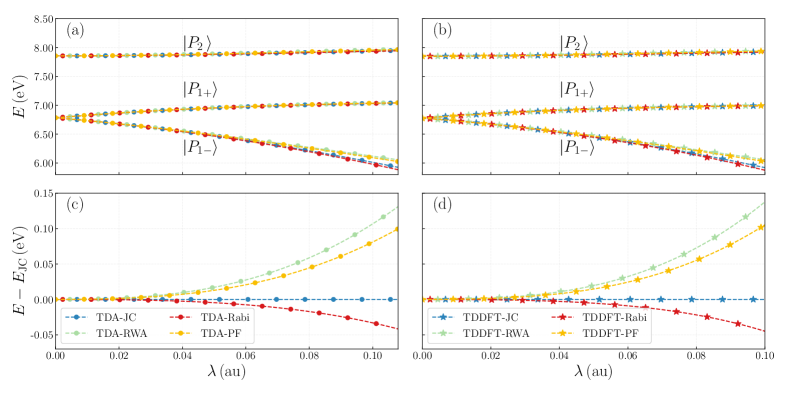
Figure 3: (a) QED-TDA and (b) QED-TDDFT polariton spectra of the formaldehyde molecule using different QED-TDDFT models with PBE0 functional and 6-311++G** basis set, as a function of the coupling strength $\lambda$. Panels (c) and (d) highlight the difference in the lower polariton energy from Rabi, RWA and PF models against corresponding TDA-JC or TDDFT-JC values.

IV.2 Formaldehyde

For the formaldehyde molecule, the TDA-JC model (marked as blue dots in Fig. 3a) yielded very similar results to that of ethene: the first excited state with a substantial oscillator strength in the gas-phase (excitation energy: $6.784\,\mathrm{eV}$; dipole: $0.490\,\mathrm{au}$) undergoes a non-symmetric Rabi splitting in the photon cavity. This happens due to a perturbation from the 4-th state (labelled as $\ket{P_{2}}$) with an excitation energy of $7.856\,\mathrm{eV}$ and a large transition dipole moment of $0.3728\,\mathrm{au}$ in the $x$-direction.

For this molecule, we would shift our attention to a comparison among the JC, Rabi, RWA, and PF variations of QED-TDA or QED-TDDFT methods. As shown in Fig 3a, when the coupling strength is small, the four variations produce very similar energy spectra. In fact, at $\lambda=0.045\,\mathrm{au}$, the predicted Rabi splitting differ by no more than $0.02\,\mathrm{eV}$ among the four models.

When the coupling strength further increases, the four models still yield nearly identical energies for the upper polariton, $\ket{P_{1+}}$. However, the predicted energies for the lower polariton, $\ket{P_{1-}}$, start to exhibit noticeable differences (Fig 3a). This is more clear in Fig 3c, which shows the energy differences against the TDA-JC model. The TDA-Rabi model (marked red), which adds the CRT term to TDA-JC, lowers the polariton energy in an agreement with the leading perturbative correction in Eq. 19. Meanwhile, the TDA-RWA model (illustrated as green dots) captures the DSE contribution missing in the TDA-JC model and thus raises the polariton energy in consistence with Eq.17. At large $\lambda$ values, the CRT correction to TDA-JC model is found to be 3–4 times smaller than the DSE correction, in terms of the absolute value. For the TDA-PF model (marked yellow in Fig 3b), which adds both CRT and DSE corrections to the TDA-JC model, the CRT term only partially cancelled the DSE component, also leading to a net energy increase.

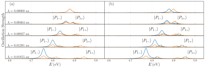
Figure 4: Absorption spectra of the benzaldehyde molecule from TDA-JC (solid lines) and 2-state Jaynes-Cummings model (dot-dashed lines) calculations with different coupling strengthes using the PBE0 functional and 6-311++G** basis set. Fabry-Pérot mode is chosen to be (a) in resonance ($4.879$ eV) and (b) 0.02 eV off-resonance ($4.899$ eV) from the gas-phase excited state. The blue and orange lines indicate the electron and photon contributions, respectively. Following Ref. 91, Lorentzian broadening is employed with $\Delta=10^{-2}\,\mathrm{eV}$.

At smaller $\lambda$ values, the CRT correction is found numerically to be exactly $-\frac{1}{4}$ of the DSE correction, which is consistent with our earlier analysis at the end of Subsection II.3. There we also mentioned that Huo and coworker’s prediction that the CRT correction is $-\frac{1}{2}$ of the DSE value at resonance.[52] This discrepancy is caused by a subtle difference in choosing the value of the fundamental coupling strength, $\bm{\lambda}_{\alpha}$, which is set to be $\sqrt{\frac{2}{\epsilon_{0}V_{\mathrm{eff}}}}\bm{\epsilon}_{\alpha}$ in our work but $\sqrt{\frac{1}{\epsilon_{0}V_{\mathrm{eff}}}}\bm{\epsilon}_{\alpha}$ in Ref. 52. As a result, our DSE correction in Eq. 17 is twice larger. Meanwhile, at resonance and weak coupling, the electron-photon coupling in Eq. 20 can be written as $g_{\alpha,I}=\sqrt{\frac{\omega_{\alpha}}{2\hbar}}\left(\bm{\lambda}_{\alpha}\cdot\bm{\mu}_{I}^{\textrm{TDA-JC}}\right)=\sqrt{\frac{\omega_{\alpha}}{2\hbar}}\left(\bm{\lambda}_{\alpha}\cdot\frac{1}{\sqrt{2}}\bm{\mu}_{I}^{\textrm{TDA}}\right)=\sqrt{\frac{\omega_{\alpha}}{2\hbar\epsilon_{0}V_{\mathrm{eff}}}}\left(\bm{\epsilon}_{\alpha}\cdot\bm{\mu}_{I}^{\textrm{TDA}}\right)$, which is exactly the same as Eq. 11 in Ref. 52. This led to an identical CRT correction, $-\frac{\hbar}{2\omega_{\alpha}}g_{\alpha,I}^{2}$. In choosing our value for $\bm{\lambda}_{\alpha}$, we follow Rubio,[83, 91] Subotnik,[65, 66, 67, 123] and others.[82, 98] It would be a reasonable choice when one or more molecules is placed within a horizontal plane equidistant from the two mirrors ($z=L_{z}/2$, where the sine wave reaches its maximum value). When the molecular concentration further increases, however, it might be better to follow Huo and coworkers [112, 52] and adopt a reduced $\bm{\lambda}_{\alpha}$ value to reflect a vertical molecular distribution.

While our discussion on the formaldehyde molecule has so far focused on QED-TDA calculations, all our observations on the comparison among JC, Rabi, RWA, and PF models would also apply to QED-TDDFT results displayed in Fig. 3c and  3d. Overall, with the leading contribution from CRT and DSE being second order to the coupling strength, both terms can be ignored for small coupling strengths. Namely, the TDA-JC and TDDFT-JC models can be used to describe polariton states at weak light-matter interaction regime.[113, 52] However, more caution is needed to select an appropriate model in strong and ultra-strong coupling regimes, where the lower polariton energy can become unbounded without the DSE correction.[52]

IV.3 Benzaldehyde

The TDA-JC results of the benzaldehyde molecule are presented as a more realistic example of the photochrome. (Other QED-TDDFT models are also tested and found to lead to similar results in Table S5.) In particular, the focus is placed on the second excited state from the gas-phase TDA calculation with an excitation energy of $4.879\,\mathrm{eV}$ and a transition dipole of $0.427\,\mathrm{au}$ in the $xy$–plane. In Fig 4a, this state is coupled to a resonant Fabry-Pérot mode; while in Fig 4b, it is coupled to an off-resonance cavity mode of $4.899\,\mathrm{eV}$ (i.e., a detuning of $0.02\,\mathrm{eV}$). Clearly, as the coupling strength $\lambda$ increases, larger Rabi splittings occur in both resonant and off-resonant cases. Moreover, the energies of both lower and upper polaritons deviate further away from the 2-state-predicted values (dot-dashed lines), in a way similar to the ethene and formaldehyde molecules. Interestingly, for our chosen coupling strengths, the off-resonance results in Fig. 4b show slightly smaller differences between the 2-state Jaynes-Cummings model and the TDA-JC method. This occurs because, with a detuning of 0.02 eV, the overall Rabi splitting is slightly smaller.

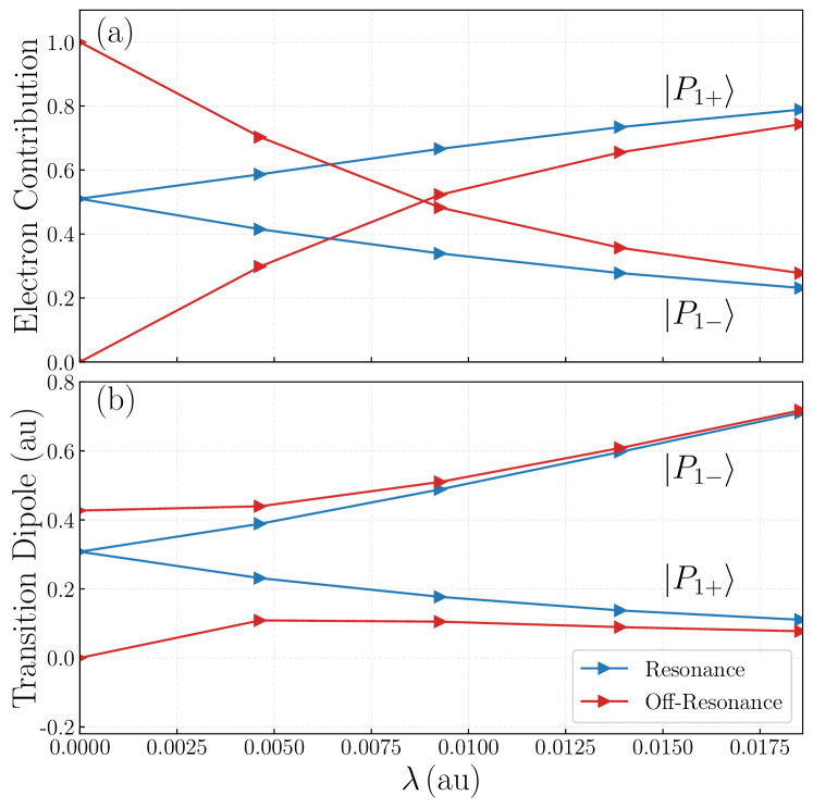
Figure 5: (a) Electron contributions and (b) the corresponding norms of transition dipole moments for the lower and upper polaritons of bezaldehyde at different coupling strengths with resonance (blue) and off-resonance (red) photon energies.

An analysis of the composition of polariton “wavefunction” of benzaldehyde leads to observations similar to the ethene molecule (Fig. 2b). At non-zero coupling strengths, the lower polariton, $\ket{P_{1-}}$, is shown in Fig. 5a to contain less electron contribution than the photon contribution, while the opposite can be seen for the upper polariton, $\ket{P_{1+}}$. Such deviations from the 2-state Jaynes-Cummings model, which would predict equal electron and photon contributions for both polaritons in a resonance coupling, can be traced to non-negligible second-order contributions from higher excited states (3rd, 5th, and 11-th states in Table S4; and many more) of gas-phase benzaldehyde. For off-resonance coupling, similar behavior can also be seen in Fig. 5b, but the lower polariton, $\ket{P_{1-}}$, contains more electron contributions (than the resonance case) due to a higher photon energy.

At first glance, smaller electronic contribution to the lower polariton with stronger electron–photon coupling as shown in Fig. 5a would appear to contradict Fig. 4a and 4b, where the TDA-JC molecular oscillation strength (marked blue) of the lower polariton actually increases with the coupling strength. To resolve such a “contradiction”, it is useful to examine the change of the molecular transition dipoles of the polaritons (as defined in Eq. S2 and S3 in the SI) with varying coupling strength. Surprisingly, as shown in Fig. 5b, the transition dipole of the lower polariton increases with larger coupling strength, while the opposite happens to the upper polariton. This can be understood within a 3–state model. Specifically, Eq. 106 indicates that the transition dipole of the lower polariton will be enhanced by those of higher-energy excited states, while the transition dipole of the upper polariton will get weakened by those states (Eq. 107). This is confirmed by Fig. S1, which shows a steady increase in the transition dipole of the lower polariton as more states are included the Jaynes-Cummings model Hamiltonian, and by an opposite trend for the upper polariton in the Figure. In the limit of strong couplings (such as $\lambda=0.01853$ au), the upper polariton state of benzaldehyde should be dominated by the $\ket{e_{1}}$ state (with the corresponding coefficient being 0.88). But due to the slow $\frac{1}{\omega_{2}-\omega}$ decay arising from Eqs. 106 and 107 and demonstrated in Fig. S1, many higher excited states (with small but nonzero mixing coefficients) combine together to cancel the $\ket{e_{1}}$ dipole moment. At $\lambda=0.01853$ au, the transition dipoles for the upper polariton is reduced by two thirds from its gas-phase value, leading to only marginal oscillator strengths in Fig. 4.

Such collective enhancement (weakening) of the lower (upper) polariton transition dipole by many higher excited states would be difficult to capture with the construction of multi-state Jaynes-Cummings model Hamiltonians. As shown in Fig. S1, with strong coupling, tens of excited states need to be included in the model before the converged value of the transition dipole moment can be approached. But it holds the key to our understanding of the absorption spectra of benzaldehyde in this work as well as other molecules displaying non-symmetric Rabi splitting, such as merocyanine in Fig. 3a of Ref.27.

V Conclusions

In summary, some progress has been made in this work on the formulation, implementation, and understanding of QED-TDDFT models, including,

• The 2-state Jaynes-Cummings model could be considered as an appropriate approximation when the coupling strength is weak enough that the higher excited states can be ignored.

• Through linear-response and equation-of-motion formulations, simple QED-TDDFT working equations are obtained for the Pauli-Fierz Hamiltonian. The Gaussian-basis implementation of the TDDFT-PF and associated approximate models paves the way for their routine applications.

• In the strong and ultra-strong coupling regime, the polaritons might get perturbed noticeably by higher excited states with significant transition dipole moments. For our test molecules, these excited states reduce the electron contribution to the lower polariton but enhance its transition dipole moment and oscillator strength, whereas they affect the upper polariton in exactly the opposite manner. While the QED-TDDFT/TDA method accounts for these effects naturally, it would be cumbersome (if feasible at all with the slow decay) to identify all these states from gas-phase calculations and then include them in the model Hamiltonian.

• At the strong coupling limit, the dipole self energy and counter rotation terms can also cause noticeable changes to the energies of polariton states.

On the other hand, within the TDDFT framework, several technical components have yet to be developed:

• In this work, the photochromes are assumed to be separated in the vacuum. To capture the effect of other molecular species in the cavity (such as PMMA or solvents), implicit solvent models or combined quantum mechanical molecular mechanical models should be adopted.

• Analytical energy derivatives are needed to allow (a) the optimization of the photochoromic geometry for different polariton states and (b) the modeling of photochemical reactions and absorption/emission spectra.

• All molecules are assumed to adopt the same orientation within the optical cavity. Our models need to be extended to cases where molecules adopt random orientations.

Work along these lines is expected to be rather straightforward and will be reported in subsequent publications.

Data Availability

The data that support the findings of this study are available from one of the corresponding authors (YS) upon reasonable request. The code implementation will be made available through PySCF and Q-Chem.

Appendix A Linear-Response Derivation

In this section, we present a matrix derivation of the QED-TDDFT equations, which closely follows Rubio and coworkers’ approach based on linear-response formula.[82, 83, 84, 86, 94, 89, 95, 96]

A.1 Density Response Kernel

For a KS-DFT electronic ground-state, its Fock matrix (i.e. effective one-electron Hamiltonian) is diagonal in the representation of Kohn-Sham orbitals,

$$\mathbf{F}_{0}=\begin{bmatrix}\mathbf{F}_{\textrm{oo}}&\mathbf{0}\\ \mathbf{0}&\mathbf{F}_{\textrm{vv}}\end{bmatrix}$$ (22)

with $F_{ij}=\varepsilon_{i}\delta_{ij}$ and $F_{ab}=\varepsilon_{a}\delta_{ab}$. The density matrix takes the format,

$$\mathbf{P}_{0}=\begin{bmatrix}\mathbf{I}_{\textrm{oo}}&\mathbf{0}\\ \mathbf{0}&\mathbf{0}\end{bmatrix}$$ (23)

with a single occupancy for the lowest-energy spin orbitals.

Within the matrix formulation of TDDFT, the Fock matrix is subjected to a frequency-dependent perturbation,

$$\mathbf{F}(t) = \mathbf{F}_{0}+\delta\mathbf{F}(t)$$ (24)

$$\delta\mathbf{F}(t) = \begin{bmatrix}\mathbf{0}&\delta\mathbf{F}_{\textrm{ov}}^{(\Omega)}e^{i\Omega t}\\ \delta\mathbf{F}_{\textrm{vo}}^{(\Omega)}e^{-i\Omega t}&\mathbf{0}\end{bmatrix}$$ (25)

$$+\begin{bmatrix}\mathbf{0}&\delta\mathbf{F}_{\textrm{ov}}^{(-\Omega)}e^{-i\Omega t}\\ \delta\mathbf{F}_{\textrm{vo}}^{(-\Omega)}e^{i\Omega t}&\mathbf{0}\end{bmatrix}$$

where $\delta\mathbf{F}_{\textrm{ov}}^{(\Omega)}=\delta\mathbf{F}_{\textrm{vo}}^{(\Omega),\dagger}$ and $\delta\mathbf{F}_{\textrm{ov}}^{(-\Omega)}=\delta\mathbf{F}_{\textrm{vo}}^{(-\Omega),\dagger}$ to maintain a Hermitian matrix. Such a perturbation causes a response in the density matrix,

$$\mathbf{P}(t) = \mathbf{P}_{0}+\delta\mathbf{P}(t)$$ (26)

$$\delta\mathbf{P}(t) = \begin{bmatrix}\mathbf{0}&\delta\mathbf{P}_{\textrm{ov}}^{(\Omega)}e^{i\Omega t}\\ \delta\mathbf{P}_{\textrm{vo}}^{(\Omega)}e^{-i\Omega t}&\mathbf{0}\end{bmatrix}$$ (27)

$$+\begin{bmatrix}\mathbf{0}&\delta\mathbf{P}_{\textrm{ov}}^{(-\Omega)}e^{-i\Omega t}\\ \delta\mathbf{P}_{\textrm{vo}}^{(-\Omega)}e^{i\Omega t}&\mathbf{0}\end{bmatrix}$$

where $\delta\mathbf{P}_{\textrm{ov}}^{(\Omega)}=\delta\mathbf{P}_{\textrm{vo}}^{(\Omega),\dagger}$ and $\delta\mathbf{P}_{\textrm{ov}}^{(-\Omega)}=\delta\mathbf{P}_{\textrm{vo}}^{(-\Omega),\dagger}$.

The density response is governed by the time-dependent Kohn-Sham (TDKS) equation,[101, 103, 105, 108]

$$i\hbar\frac{\partial\mathbf{P}(t)}{\partial t} = [\mathbf{F}(t),\mathbf{P}(t)]=[\delta\mathbf{F}(t),\mathbf{P}_{0}]+[\mathbf{F}_{0},\delta\mathbf{P}(t)]$$ (28)

which is

$$i\hbar\frac{\partial\mathbf{P}(t)}{\partial t}=\begin{bmatrix}\mathbf{0}&-\delta\mathbf{F}_{\textrm{ov}}\\ \delta\mathbf{F}_{\textrm{vo}}&\mathbf{0}\end{bmatrix}$$

$$+\begin{bmatrix}\mathbf{0}&\mathbf{F}_{\textrm{oo}}\delta\mathbf{P}_{\textrm{ov}}-\delta\mathbf{P}_{\textrm{ov}}\mathbf{F}_{\textrm{vv}}\\ \mathbf{F}_{\textrm{vv}}\delta\mathbf{P}_{\textrm{vo}}-\delta\mathbf{P}_{\textrm{vo}}\mathbf{F}_{\textrm{oo}}&\mathbf{0}\end{bmatrix}$$ (29)

Below we shall focus on the vo-block of this equation, which requires

$$i\hbar\frac{\partial\mathbf{P}_{\textrm{vo}}(t)}{\partial t}=\delta\mathbf{F}_{\textrm{vo}}+\mathbf{F}_{\textrm{vv}}\delta\mathbf{P}_{\textrm{vo}}-\delta\mathbf{P}_{\textrm{vo}}\mathbf{F}_{\textrm{oo}},$$ (30)

noting that the ov-block equation is the complex conjugate.

Collecting the $e^{-i\Omega t}$ and $e^{i\Omega t}$ terms separately from both sides of Eq. 30, one gets

$$(\hbar\Omega)\delta\mathbf{P}_{\textrm{vo}}^{(\Omega)} = \delta\mathbf{F}_{\textrm{vo}}^{(\Omega)}+\mathbf{F}_{\textrm{vv}}\delta\mathbf{P}_{\textrm{vo}}^{(\Omega)}-\delta\mathbf{P}_{\textrm{vo}}^{(\Omega)}\mathbf{F}_{\textrm{oo}}$$ (31)

$$(-\hbar\Omega)\delta\mathbf{P}_{\textrm{vo}}^{(-\Omega)} = \delta\mathbf{F}_{\textrm{vo}}^{(-\Omega)}+\mathbf{F}_{\textrm{vv}}\delta\mathbf{P}_{\textrm{vo}}^{(-\Omega)}-\delta\mathbf{P}_{\textrm{vo}}^{(-\Omega)}\mathbf{F}_{\textrm{oo}}$$

which can be written explicitly as

$$(\hbar\Omega-\varepsilon_{a}+\varepsilon_{i})\delta P_{ai}^{(\Omega)} = \delta F_{ai}^{(\Omega)}$$ (33)

$$(-\hbar\Omega-\varepsilon_{a}+\varepsilon_{i})\delta P_{ai}^{(-\Omega)} = \delta F_{ai}^{(-\Omega)}$$ (34)

This shows how the density matrix would respond to a frequency-dependent change in the Fock matrix.

A.2 Electron Equations within QED-TDDFT

For a molecule in an optical cavity, its Fock matrix is influenced by changes in both the electronic density matrix in Eq. 27 as well as the electron-photon coupling,

$$\delta F_{ai}^{(\Omega)} = \delta F_{ai,\textrm{elec}}^{(\Omega)}+\delta F_{ai,\textrm{elec-photon}}^{(\Omega)}$$ (35)

$$\delta F_{ai}^{(-\Omega)} = \delta F_{ai,\textrm{elec}}^{(-\Omega)}+\delta F_{ai,\textrm{elec-photon}}^{(-\Omega)}$$ (36)

For $F_{ai}^{(\Omega)}$, it is only perturbed by $P_{bj}^{(\Omega)}$ and $P_{jb}^{(-\Omega)}$, which carry the same $e^{-i\Omega t}$ factor in Eq. 27,

$$\delta F_{ai,\textrm{elec}}^{(\Omega)}=\sum_{bj}\left(\frac{\partial F_{ai}}{\partial P_{bj}}\delta P_{bj}^{(\Omega)}+\frac{\partial F_{ai}}{\partial P_{jb}}\delta P_{jb}^{(-\Omega)}\right)$$

$$=\sum_{bj}\left[\left[A_{ai,bj}-(\varepsilon_{a}-\varepsilon_{i})\delta_{ab}\delta_{ij}\right]\delta P_{bj}^{(\Omega)}+B_{ai,bj}\delta P_{jb}^{(-\Omega)}\right]$$ (37)

Similarly, for $F_{ai,\textrm{elec}}^{(-\Omega)}$, one gets

$$\delta F_{ai,\textrm{elec}}^{(-\Omega)}=\sum_{bj}\left(\frac{\partial F_{ai}}{\partial P_{bj}}\delta P_{bj}^{(-\Omega)}+\frac{\partial F_{ai}}{\partial P_{jb}}\delta P_{jb}^{(\Omega)}\right)$$

$$=\sum_{bj}\left[\left[A_{ai,bj}-(\varepsilon_{a}-\varepsilon_{i})\delta_{ab}\delta_{ij}\right]\delta P_{bj}^{(-\Omega)}+B_{ai,bj}\delta P_{jb}^{(\Omega)}\right]$$ (38)

For the electron-photon interaction energy in Eq. 7,

$$V_{\textrm{elec-photon}}=\sum_{\alpha=1}^{M}\frac{1}{2}\omega_{\alpha}^{2}\left(q_{\alpha}-\frac{1}{\omega_{\alpha}}\bm{\lambda}_{\alpha}\cdot\bm{\mu}\right)^{2}$$ (39)

its corresponding Fock matrix contribution is

$$F_{ai,\textrm{elec-photon}}=\frac{\partial V_{\textrm{elec-photon}}}{\partial P_{ai}}$$

$$=\sum_{\alpha=1}^{M}\omega_{\alpha}\lambda_{ai}^{\alpha}\left(q_{\alpha}-\frac{1}{\omega_{\alpha}}\bm{\lambda}_{\alpha}\cdot\bm{\mu}\right)$$ (40)

which uses the dipole derivative

$$\frac{\partial\bm{\mu}}{\partial P_{ai}}=\frac{\partial\left(\bm{\mu}_{\textrm{nuc}}-\bm{\mu}_{\textrm{mo}}\cdot\mathbf{P}\right)}{\partial P_{ai}}=-\bm{\mu}_{ai}$$ (41)

Clearly, the Fock matrix contribution in Eq. 40 is perturbed by the density matrix and photon coordinate,

$$\delta F_{ai,\textrm{elec-photon}}^{(\Omega)}=\delta F_{ai,\textrm{elec-photon}}^{(-\Omega)}$$

$$=\sum_{bj}\left(\sum_{\alpha=1}^{M}\lambda_{ai}^{\alpha}\lambda_{bj}^{\alpha}\right)\left(\delta P_{bj}^{(\Omega)}+\delta P_{jb}^{(-\Omega)}\right)+\sum_{\alpha=1}^{M}\omega_{\alpha}\lambda_{ai}^{\alpha}\delta q_{\alpha}$$

$$=\sum_{bj}\Delta_{ai,bj}\left(\delta P_{bj}^{(\Omega)}+\delta P_{jb}^{(-\Omega)}\right)$$

$$\quad+\sum_{\alpha=1}^{M}\sqrt{\frac{\hbar\omega_{\alpha}}{2}}\lambda_{ai}^{\alpha}\left(M_{\alpha}+N_{\alpha}\right)$$ (42)

which uses the expression of $\Delta_{ai,bj}$ in Eq. 9 and replaces $\delta\hat{q}_{\alpha}$ with dimensional quantities,

$$\delta q_{\alpha}=\sqrt{\frac{\hbar}{2\omega_{\alpha}}}\left(M_{\alpha}+N_{\alpha}\right)$$ (43)

Plugging Eqs. 37, 38 and 42 into the right-hand-side of Eqs. 33 and 34, one obtains

$$(\hbar\Omega)\delta P_{ai}^{(\Omega)}=\sum_{bj}\left(A_{ai,bj}+\Delta_{ai,bj}\right)\delta P_{bj}^{(\Omega)}$$

$$\quad+\sum_{bj}\left(B_{ai,bj}+\Delta_{ai,bj}\right)\delta P_{jb}^{(-\Omega)}$$

$$\quad+\sum_{\alpha=1}^{M}\sqrt{\frac{\hbar\omega_{\alpha}}{2}}\lambda_{ai}^{\alpha}\left(M_{\alpha}+N_{\alpha}\right)$$ (44)

$$(-\hbar\Omega)\delta P_{ai}^{(-\Omega)}=\sum_{bj}\left(A_{ai,bj}+\Delta_{ai,bj}\right)\delta P_{bj}^{(-\Omega)}$$

$$\quad+\sum_{bj}\left(B_{ai,bj}+\Delta_{ai,bj}\right)\delta P_{jb}^{(\Omega)}$$

$$\quad+\sum_{\alpha=1}^{M}\sqrt{\frac{\hbar\omega_{\alpha}}{2}}\lambda_{ai}^{\alpha}\left(M_{\alpha}+N_{\alpha}\right)$$ (45)

Assume that $\delta P_{ai}^{(\Omega)}=\delta P_{ia}^{(\Omega)}$ and $\delta P_{ai}^{(-\Omega)}=\delta P_{ia}^{(-\Omega)}$ are all real, and write them as $X_{ai}$ and $Y_{ai}$, respectively, we obtain the electronic portion of the QED-TDDFT equation in Eq. 8.

A.3 Photon Equations within QED-TDDFT

The photon equation of state is[91]

$$\left(\frac{\partial^{2}}{\partial t^{2}}+\omega_{\alpha}^{2}\right)q_{\alpha}(t)=-\frac{1}{\omega_{\alpha}}j_{\alpha}^{\textrm{eff}}(t)$$

$$\quad\quad=-\frac{1}{\omega_{\alpha}}\left(j_{\alpha}(t)-\omega_{\alpha}^{2}\bm{\lambda}_{\alpha}\cdot\bm{\mu}\right)$$ (46)

For $q_{\alpha}(t)$ and $j_{\alpha}^{\textrm{eff}}(t)$ oscillating with frequency $\Omega$, they satisfy

$$\left(\Omega^{2}-\omega_{\alpha}^{2}\right)\delta q_{\alpha}=\frac{1}{\omega_{\alpha}}\delta j_{\alpha}^{\textrm{eff}}$$ (47)

Therefore, the photon response is

$$\delta q_{\alpha} = \frac{1}{\omega_{\alpha}}\frac{1}{\Omega^{2}-\omega_{\alpha}^{2}}\delta j_{\alpha}^{\textrm{eff}}$$ (48)

$$= \frac{1}{2\omega_{\alpha}^{2}}\left(\frac{1}{\Omega-\omega_{\alpha}}-\frac{1}{\Omega+\omega_{\alpha}}\right)\delta j_{\alpha}^{\textrm{eff}}$$

A key to the QED-TDDFT method is the splitting of the right-hand-side,[91] which underlies Eq. 43,

$$\left(\hbar\Omega-\hbar\omega_{\alpha}\right)M_{\alpha}=\sqrt{\frac{\hbar}{2\omega_{\alpha}^{3}}}\delta j_{\alpha}^{\textrm{eff}}$$ (49)

$$-\left(\hbar\Omega+\hbar\omega_{\alpha}\right)N_{\alpha}=\sqrt{\frac{\hbar}{2\omega_{\alpha}^{3}}}\delta j_{\alpha}^{\textrm{eff}}$$ (50)

where $\delta j_{\alpha}^{\textrm{eff}}$ can be easily derived from Eq. 46,

$$\delta j_{\alpha}^{\textrm{eff},(\Omega)} = \omega_{\alpha}^{2}\sum_{bj}\lambda_{bj}^{\alpha}\left(\delta P_{bj}^{(\Omega)}+\delta P_{jb}^{(-\Omega)}\right)$$ (51)

Therefore,

$$(\hbar\Omega)M_{\alpha}=\sum_{bj}\sqrt{\frac{\hbar\omega_{\alpha}}{2}}\lambda_{bj}^{\alpha}\left(\delta P_{bj}^{(\Omega)}+\delta P_{jb}^{(-\Omega)}\right)+(\hbar\omega_{\alpha})M_{\alpha}$$ (52)

$$-(\hbar\Omega)N_{\alpha}=\sum_{bj}\sqrt{\frac{\hbar\omega_{\alpha}}{2}}\lambda_{bj}^{\alpha}\left(\delta P_{bj}^{(\Omega)}+\delta P_{jb}^{(-\Omega)}\right)+(\hbar\omega_{\alpha})N_{\alpha}$$ (53)

which are the photon portion of Eq. 8.

Appendix B Equation-of-Motion Derivation

Below, we shall use an alternative approach, which based on the equation-of-motion by transforming into a Heisenberg picture, to derive the same QED-TDDFT equation in Eq. 8. [109, 110, 111] Within this derivation, the split of $q_{\alpha}$ in Eq. 43 will come naturally.

B.1 Unitary Transformation of Electronic Wavefunction

The electronic wavefunction evolves with an unitary transformation

$$\left|\Phi(t)\right> = e^{-\hat{\Lambda}_{\textrm{e}}(t)}\left|\Phi_{0}\right>$$ (54)

$$\hat{\Lambda}_{\textrm{e}}(t) = \sum_{ai}\left(-\Theta_{ai}^{\ast}(t)\hat{a}_{i}^{\dagger}\hat{a}_{a}+\Theta_{ai}(t)\hat{a}_{a}^{\dagger}\hat{a}_{i}\right)$$ (55)

Using the following commutators,[109]

$$\left[\hat{a}_{a}^{\dagger}\hat{a}_{i},\hat{a}_{j}^{\dagger}\hat{a}_{b}\right] = \delta_{ij}\hat{a}_{a}^{\dagger}\hat{a}_{b}-\delta_{ab}\hat{a}_{j}^{\dagger}\hat{a}_{i}$$ (56)

$$\left[\hat{a}_{a}^{\dagger}\hat{a}_{i},\hat{a}_{b}^{\dagger}\hat{a}_{j}\right] = \left[\hat{a}_{i}^{\dagger}\hat{a}_{a},\hat{a}_{j}^{\dagger}\hat{a}_{b}\right]=0$$ (57)

one can find

$$\left[\hat{\Lambda}_{\textrm{e}},\hat{a}_{j}^{\dagger}\hat{a}_{b}\right] = \sum_{a}\Theta_{aj}(t)\hat{a}_{a}^{\dagger}\hat{a}_{b}-\sum_{i}\Theta_{bi}(t)\hat{a}_{j}^{\dagger}\hat{a}_{i}$$ (58)

$$\left[\hat{\Lambda}_{\textrm{e}},\hat{a}_{b}^{\dagger}\hat{a}_{j}\right] = \sum_{a}\Theta_{aj}^{*}(t)\hat{a}_{b}^{\dagger}\hat{a}_{a}-\sum_{i}\Theta_{bi}^{*}(t)\hat{a}_{i}^{\dagger}\hat{a}_{j}$$ (59)

Using the leading terms of the following BCH expansion,

$$e^{\hat{\Lambda}_{\textrm{e}}}\left(\hat{a}_{j}^{\dagger}\hat{a}_{b}+\hat{a}_{b}^{\dagger}\hat{a}_{j}\right)e^{-\hat{\Lambda}_{\textrm{e}}}=\hat{a}_{j}^{\dagger}\hat{a}_{b}+\hat{a}_{b}^{\dagger}\hat{a}_{j}$$

$$+\sum_{a}\left(\Theta_{aj}(t)\hat{a}_{a}^{\dagger}\hat{a}_{b}+\Theta_{aj}^{*}(t)\hat{a}_{b}^{\dagger}\hat{a}_{a}\right)$$

$$-\sum_{i}\left(\Theta_{bi}(t)\hat{a}_{j}^{\dagger}\hat{a}_{i}+\Theta_{bi}^{*}(t)\hat{a}_{i}^{\dagger}\hat{a}_{j}\right)+\mathcal{O}(\Theta^{2})$$ (60)

one finds

$$\left<\Phi(t)\middle|\left(\hat{a}_{j}^{\dagger}\hat{a}_{b}+\hat{a}_{b}^{\dagger}\hat{a}_{j}\right)\middle|\Phi(t)\right>$$

$$=\left<\Phi_{0}\middle|e^{\hat{\Lambda}_{\textrm{e}}}\left(\hat{a}_{j}^{\dagger}\hat{a}_{b}+\hat{a}_{b}^{\dagger}\hat{a}_{j}\right)e^{-\hat{\Lambda}_{\textrm{e}}}\middle|\Phi_{0}\right>=-\Theta_{bj}(t)-\Theta_{bj}^{*}(t)$$ (61)

B.2 Unitary Transformation of Photon Wavefunction

Similarly, the photon wavefunction is also subjected to an unitary transformation (Eq. 26 in Ref. 97)

$$\left|\chi(t)\right> = e^{-\hat{\Lambda}_{\textrm{ph}}(t)}\left|\Phi_{0}\right>\left|\chi_{0}\right>$$ (62)

$$\hat{\Lambda}_{\textrm{ph}}(t) = \sum_{\alpha}\left(-C_{\alpha}^{*}(t)\hat{b}_{\alpha}+C_{\alpha}(t)\hat{b}_{\alpha}^{\dagger}\right)$$ (63)

Using the commutators for bosons,

$$\left[\hat{b}_{\alpha},\hat{b}_{\beta}^{\dagger}\right]=\delta_{\alpha\beta},\quad\left[\hat{b}_{\alpha},\hat{b}_{\beta}\right]=\left[\hat{b}_{\alpha}^{\dagger},\hat{b}_{\beta}^{\dagger}\right]=0$$ (64)

one gets

$$\left[\hat{\Lambda}_{\textrm{ph}},\hat{b}_{\alpha}\right]=-C_{\alpha}(t),\quad\quad\left[\hat{\Lambda}_{\textrm{ph}},\hat{b}_{\alpha}^{\dagger}\right]=-C_{\alpha}^{*}(t)$$ (65)

Accordingly, the following BCH expansions vanish after the first order

$$e^{\hat{\Lambda}_{\textrm{ph}}}\hat{b}_{\alpha}e^{-\hat{\Lambda}_{\textrm{ph}}}=\hat{b}_{\alpha}-C_{\alpha}(t)$$ (66)

$$e^{\hat{\Lambda}_{\textrm{ph}}}\hat{b}_{\alpha}^{\dagger}e^{-\hat{\Lambda}_{\textrm{ph}}}=\hat{b}_{\alpha}^{\dagger}-C_{\alpha}^{*}(t)$$ (67)

From this, one can compute

$$\left<\chi(t)\middle|\left(\hat{b}_{\alpha}+\hat{b}_{\alpha}^{\dagger}\right)\middle|\chi(t)\right>=-C_{\alpha}(t)-C_{\alpha}^{*}(t)$$ (68)

$$\left<\chi(t)\middle|\hat{b}_{\alpha}^{\dagger}\hat{b}_{\alpha}\middle|\chi(t)\right>$$

$$=\left<\chi_{0}\middle|\left(e^{\hat{\Lambda}_{\textrm{ph}}}\hat{b}_{\alpha}^{\dagger}e^{-\hat{\Lambda}_{\textrm{ph}}}\right)\left(e^{\hat{\Lambda}_{\textrm{ph}}}\hat{b}_{\alpha}e^{-\hat{\Lambda}_{\textrm{ph}}}\right)\middle|\chi_{0}\right>=C_{\alpha}(t)C_{\alpha}^{*}(t)$$ (69)

B.3 Pauli-Fierz Energy Components

In the Pauli-Fierz Hamiltonian in Eq. 7, the dipole moment operator can be written as

$$\hat{\bm{\mu}}=\bm{\mu}_{0}+\Delta\hat{\bm{\mu}}=\bm{\mu}_{0}-\sum_{bj}\bm{\mu}_{bj}\left(\hat{a}_{j}^{\dagger}\hat{a}_{b}+\hat{a}_{b}^{\dagger}\hat{a}_{j}\right)$$ (70)

$$\bm{\lambda}_{\alpha}\cdot\hat{\bm{\mu}}=\bm{\lambda}_{\alpha}\cdot\bm{\mu}_{0}-\sum_{bj}\lambda_{bj}^{\alpha}\left(\hat{a}_{j}^{\dagger}\hat{a}_{b}+\hat{a}_{b}^{\dagger}\hat{a}_{j}\right)$$ (71)

where the ground-state dipole moment shifts the minimum of the quantum harmonic oscillator of the photon, $\hat{q}_{\alpha}\longrightarrow\hat{q}_{\alpha}-\frac{1}{\omega_{\alpha}}\bm{\lambda}_{\alpha}\cdot\bm{\mu}_{0}$. Then, the Pauli-Fierz Hamiltonian can be written as

$$\hat{H}_{\textrm{PF}} = \hat{H}_{\mathrm{elec}}(t)+\frac{1}{2}\sum_{\alpha=1}^{M}\left(\bm{\lambda}_{\alpha}\cdot\left<\Delta\hat{\bm{\mu}}\right>\right)^{2}$$ (72)

$$-\sum_{\alpha=1}^{M}\omega_{\alpha}\hat{q}_{\alpha}\left(\bm{\lambda}_{\alpha}\cdot\left<\Delta\hat{\bm{\mu}}\right>\right)$$

$$+\sum_{\alpha=1}^{M}\left[\frac{1}{2}\hat{p}_{\alpha}^{2}+\frac{1}{2}\omega_{\alpha}^{2}\hat{q}_{\alpha}^{2}\right]+\sum_{\alpha=1}^{M}\frac{j_{\alpha}(t)}{\omega_{\alpha}}\hat{q}_{\alpha}\quad\quad\quad$$

With this Hamiltonian, the energy of the time-evolving wavefunction is

$$E_{\textrm{PF}}(\bm{\Theta},\mathbf{C})=\left<\chi(t)\middle|\left<\Phi(t)\middle|\hat{H}_{\textrm{PF}}\middle|\chi(t)\right>\middle|\chi(t)\right>$$ (73)

Its electronic component is[110, 109, 111]

$$\left<\chi(t)\middle|\left<\Phi(t)\middle|\hat{H}_{\textrm{elec}}\middle|\Phi(t)\right>\middle|\chi(t)\right>=\left<\Phi(t)\middle|\hat{H}_{\textrm{elec}}\middle|\Phi(t)\right>$$

$$=E_{0}+\frac{1}{2}\sum_{ai,bj}\left(\Theta_{ai}^{\ast}A_{ai,bj}\Theta_{bj}+\Theta_{ai}A_{ai,bj}\Theta_{bj}^{\ast}\right.$$

$$\quad\quad\quad\quad+\left.\Theta_{ai}B_{ai,bj}\Theta_{bj}+\Theta_{ai}^{\ast}B_{ai,bj}\Theta_{bj}^{\ast}\right)$$ (74)

while the DSE contribution is

$$\left<\chi(t)\middle|\left<\Phi(t)\middle|\frac{1}{2}\sum_{\alpha=1}^{M}\left(\bm{\lambda}_{\alpha}\cdot\left<\Delta\hat{\bm{\mu}}\right>\right)^{2}\middle|\Phi(t)\right>\middle|\chi(t)\right>$$

$$=\frac{1}{2}\sum_{\alpha=1}^{M}\left<\Phi(t)\middle|\left(\bm{\lambda}_{\alpha}\cdot\left<\Delta\hat{\bm{\mu}}\right>\right)^{2}\middle|\Phi(t)\right>$$

$$=\frac{1}{2}\sum_{\alpha,ai,bj}\lambda_{ai}^{\alpha}\lambda_{bj}^{\alpha}\left<\Phi_{0}\middle|e^{\hat{\Lambda}_{\textrm{e}}}\left(\hat{a}_{i}^{\dagger}\hat{a}_{a}+\hat{a}_{a}^{\dagger}\hat{a}_{i}\right)e^{-\hat{\Lambda}_{\textrm{e}}}\middle|\Phi_{0}\right>$$

$$\times\left<\Phi_{0}\middle|e^{\hat{\Lambda}_{\textrm{e}}}\left(\hat{a}_{j}^{\dagger}\hat{a}_{b}+\hat{a}_{b}^{\dagger}\hat{a}_{j}\right)e^{-\hat{\Lambda}_{\textrm{e}}}\middle|\Phi_{0}\right>$$

$$=\frac{1}{2}\sum_{ai,bj}\Delta_{ai,bj}\left(\Theta_{ai}(t)+\Theta_{ai}^{*}(t)\right)\left(\Theta_{bj}(t)+\Theta_{bj}^{*}(t)\right)$$ (75)

which uses the expressions in Eqs. 71 and 61.

The electron-photon coupling energy is

$$-\left<\chi(t)\middle|\left<\Phi(t)\middle|\sum_{\alpha=1}^{M}\omega_{\alpha}\hat{q}_{\alpha}\left(\bm{\lambda}_{\alpha}\cdot\left<\Delta\hat{\bm{\mu}}\right>\right)\middle|\Phi(t)\right>\middle|\chi(t)\right>$$

$$=-\sum_{\alpha=1}^{M}\omega_{\alpha}\left<\chi(t)\middle|\hat{q}_{\alpha}\middle|\chi(t)\right>\left<\Phi(t)\middle|\left(\bm{\lambda}_{\alpha}\cdot\Delta\hat{\bm{\mu}}\right)\middle|\Phi(t)\right>$$

$$=\sum_{\alpha,bj}\sqrt{\frac{\hbar\omega_{\alpha}}{2}}\left[C_{\alpha}(t)+C_{\alpha}^{*}(t)\right]\lambda_{bj}^{\alpha}\left(\Theta_{bj}(t)+\Theta_{bj}^{*}(t)\right)$$ (76)

which uses the definition of photon coordinate in Eq. 4 and the expression in Eq. 68.

Finally, from Eq. 69, the photon energy can be found to be

$$\left<\chi(t)\middle|\left<\Phi(t)\middle|\sum_{\alpha=1}^{M}\left[\frac{1}{2}\hat{p}_{\alpha}^{2}+\frac{1}{2}\omega_{\alpha}^{2}\hat{q}_{\alpha}^{2}\right]\middle|\Phi(t)\right>\middle|\chi(t)\right>$$

$$=\sum_{\alpha=1}^{M}\left<\chi(t)\middle|\left[\frac{1}{2}\hat{p}_{\alpha}^{2}+\frac{1}{2}\omega_{\alpha}^{2}\hat{q}_{\alpha}^{2}\right]\middle|\chi(t)\right>$$

$$=\sum_{\alpha=1}^{M}\hbar\omega_{\alpha}\left<\chi(t)\middle|\left[\hat{b}_{\alpha}^{\dagger}\hat{b}_{\alpha}+\frac{1}{2}\right]\middle|\chi(t)\right>$$

$$=\sum_{\alpha=1}^{M}\hbar\omega_{\alpha}\left[C_{\alpha}(t)C_{\alpha}^{*}(t)+\frac{1}{2}\right]$$ (77)

Putting these together, we will get the following derivatives

$$\frac{\partial E_{\textrm{PF}}}{\partial\Theta_{ai}} = \sum_{bj}\left[\left(A+\Delta\right)_{ai,bj}\Theta_{bj}^{\ast}(t)+\left(B+\Delta\right)_{ai,bj}\Theta_{bj}(t)\right]$$ (78)

$$+\hbar g_{ai}^{\alpha}\left[C_{\alpha}(t)+C_{\alpha}^{*}(t)\right]$$

$$\frac{\partial E_{\textrm{PF}}}{\partial C_{\alpha}} = \sum_{bj}\hbar g_{bj}^{\alpha}\left(\Theta_{bj}(t)+\Theta_{bj}^{*}(t)\right)$$ (79)

$$+\hbar\omega_{\alpha}C_{\alpha}^{*}(t)$$

B.4 Equations of Motion

Let expand the Lagrangian to first-order

$$\mathcal{L} = \left<\chi(t)\middle|\left<\Phi(t)\middle|i\hbar\frac{\partial}{\partial t}-\hat{H}_{\textrm{PF}}\middle|\Phi(t)\right>\middle|\chi(t)\right>$$ (80)

$$= i\sum_{ai}\Theta_{ai}^{\ast}(t)\frac{\partial}{\partial t}\Theta_{ai}(t)+i\hbar\sum_{\alpha}C_{\alpha}^{*}(t)\frac{\partial}{\partial t}C_{\alpha}(t)$$

$$-E_{\textrm{PF}}(\bm{\Theta}(t),\mathbf{C}(t))$$

The equation-of-motion for the orbital rotations is

$$-\frac{\partial}{\partial t}\left(\frac{\partial\mathcal{L}}{\partial\dot{\Theta}_{ai}}\right) = -\frac{\partial\mathcal{L}}{\partial\Theta_{ai}}$$ (81)

namely,

$$-i\hbar\frac{\partial}{\partial t}\Theta_{ai}^{\ast} = \frac{\partial E_{\textrm{PF}}}{\partial\Theta_{ai}}$$ (82)

Let us parameterize the orbital rotations as

$$\Theta_{ai}(t)=X_{ai}~{}e^{-i\Omega t}+Y_{ai}~{}e^{i\Omega t}$$ (83)

$$\Theta_{ai}^{\ast}(t)=X_{ai}~{}e^{i\Omega t}+Y_{ai}~{}e^{-i\Omega t}$$ (84)

and photon phase change as

$$C_{\alpha}(t)=M_{\alpha}~{}e^{-i\Omega t}+N_{\alpha}~{}e^{i\Omega t}$$ (85)

$$C_{\alpha}^{\ast}(t)=M_{\alpha}~{}e^{i\Omega t}+N_{\alpha}~{}e^{-i\Omega t}$$ (86)

Plugging in orbital rotation derivatives in Eq. 78, and separating the $e^{i\Omega t}$ and $e^{-i\Omega t}$ terms in Eq. 82, one gets the first two equations in Eq. 8,

$$\Omega X_{ai}=\sum_{bj}\left[\left(A+\Delta\right)_{ai,bj}X_{bj}+\left(B+\Delta\right)_{ai,bj}Y_{bj}\right]$$

$$\quad\quad+\sum_{\alpha}\hbar g_{ai}^{\alpha}\left(M_{\alpha}+N_{\alpha}\right)$$ (87)

$$-\Omega Y_{ai}=\sum_{bj}\left[\left(B+\Delta\right)_{ai,bj}X_{bj}+\left(A+\Delta\right)_{ai,bj}Y_{bj}\right]$$

$$\quad\quad+\sum_{\alpha}\hbar g_{ai}^{\alpha}\left(M_{\alpha}+N_{\alpha}\right)$$ (88)

The equation-of-motion for the photon phase is similar

$$-i\hbar\frac{\partial}{\partial t}C_{\alpha}^{\ast} = \frac{\partial E_{\textrm{PF}}}{\partial C_{\alpha}}$$ (89)

which, upon the insertion of the derivatives in Eq. 79, leads to the last two equations in Eq. 8,

$$\Omega M_{\alpha}=\sum_{bj}\hbar g_{bj}^{\alpha}\left(X+Y\right)_{bj}+\hbar\omega_{\alpha}M_{\alpha}$$ (90)

$$-\Omega N_{\alpha}=\sum_{bj}\hbar g_{bj}^{\alpha}\left(X+Y\right)_{bj}+\hbar\omega_{\alpha}N_{\alpha}$$ (91)

Appendix C 2-State and 3-State JC Models

Let us consider a two-level system made of $\ket{e_{1}}\ket{0_{\alpha}}$ and $\ket{g}\ket{1_{\alpha}}$, both of which have a resonance energy of $\hbar\omega$. The 2-state JC equation is

$$\begin{bmatrix}\hbar\omega&s\hbar g_{1}\\ s\hbar g_{1}&\hbar\omega\end{bmatrix}\begin{bmatrix}X_{1}\\ M\end{bmatrix}=\hbar\Omega\begin{bmatrix}X_{1}\\ M\end{bmatrix}$$ (92)

where a scaling factor $s$ is added to track the perturbation order. Its solutions are known to be the lower and upper polaritons

$$\ket{1_{-}} = \frac{1}{\sqrt{2}}\ket{e_{1}}\ket{0_{\alpha}}-\frac{1}{\sqrt{2}}\ket{g}\ket{1_{\alpha}}$$ (93)

$$\ket{1_{+}} = \frac{1}{\sqrt{2}}\ket{e_{1}}\ket{0_{\alpha}}+\frac{1}{\sqrt{2}}\ket{g}\ket{1_{\alpha}}$$ (94)

with the energies being

$$\hbar\Omega_{1-}=\hbar\omega-s\hbar g_{1}$$ (95)

$$\hbar\Omega_{1+}=\hbar\omega+s\hbar g_{1}$$ (96)

respectively.

Now let us introduce a third state, $\ket{e_{2}}\ket{0_{\alpha}}$, which has an energy of $\hbar\omega_{2}$ and is well separated from the two polariton states. The corresponding 3-state JC equation is

$$\begin{bmatrix}\hbar\omega_{2}&0&s\hbar g_{2}\\ 0&\hbar\omega&s\hbar g_{1}\\ s\hbar g_{2}&s\hbar g_{1}&\hbar\omega\end{bmatrix}\begin{bmatrix}X_{2}\\ X_{1}\\ M\end{bmatrix}=\hbar\Omega^{\prime}\begin{bmatrix}X_{2}\\ X_{1}\\ M\end{bmatrix}$$ (97)

Upon switching to the basis of $\left[\ket{e_{2}}\ket{0_{\alpha}},~{}~{}~{}\ket{1_{+}},~{}~{}~{}\ket{1_{-}}\right]$, the 3-state JC equation becomes

$$\begin{bmatrix}\hbar\omega_{2}&\frac{s\hbar g_{2}}{\sqrt{2}}&-\frac{s\hbar g_{2}}{\sqrt{2}}\\ \frac{s\hbar g_{2}}{\sqrt{2}}&\hbar\omega+s\hbar g_{1}&0\\ -\frac{s\hbar g_{2}}{\sqrt{2}}&0&\hbar\omega-s\hbar g_{1}\end{bmatrix}\begin{bmatrix}X_{2}\\ P_{1+}\\ P_{1-}\end{bmatrix}=\hbar\Omega^{\prime}\begin{bmatrix}X_{2}\\ P_{1+}\\ P_{1-}\end{bmatrix}$$ (98)

We can get the second-order perturbation to the energy of upper and lower polaritons as

$$\hbar\Omega^{\prime}_{1-}=\hbar\omega-s\hbar g_{1}-\frac{\frac{1}{2}s^{2}\hbar^{2}g_{2}^{2}}{\hbar\omega_{2}-(\hbar\omega-s\hbar g_{1})}+\cdots$$ (99)

$$\hbar\Omega^{\prime}_{1+}=\hbar\omega+s\hbar g_{1}-\frac{\frac{1}{2}s^{2}\hbar^{2}g_{2}^{2}}{\hbar\omega_{2}-(\hbar\omega+s\hbar g_{1})}+\cdots$$ (100)

To the second order of $s$, we thus have

$$\hbar\Omega^{\prime}_{1-}=\hbar\omega-s\hbar g_{1}-s^{2}\frac{\hbar^{2}g_{2}^{2}}{2(\hbar\omega_{2}-\hbar\omega)}+\mathcal{O}(s^{3})$$ (101)

$$\hbar\Omega^{\prime}_{1+}=\hbar\omega+s\hbar g_{1}-s^{2}\frac{\hbar^{2}g_{2}^{2}}{2(\hbar\omega_{2}-\hbar\omega)}+\mathcal{O}(s^{3})$$ (102)

Within the perturbation theory, the lower polariton wavefunction becomes

$$\ket{1_{-}}^{\prime}=\ket{1_{-}}^{(0)}+\ket{1_{-}}^{(1)}+\ket{1_{-}}^{(2)}+\cdots$$

$$\quad=\ket{1_{-}}+\frac{-s\hbar g_{2}/\sqrt{2}}{(\hbar\omega-s\hbar g_{1})-\hbar\omega_{2}}\ket{e_{2}}\ket{0_{\alpha}}$$

$$\quad+\frac{-\frac{1}{2}s^{2}\hbar^{2}g_{2}^{2}}{(-2s\hbar g_{1})\left[(\hbar\omega-s\hbar g_{1})-\hbar\omega_{2}\right]}\ket{1_{+}}+\cdots$$ (103)

Plugging in the expressions in Eqs. 93 and 94 and truncating at the first order of $s$, one gets

$$\ket{1_{-}}^{\prime} = -\frac{1}{\sqrt{2}}\left(1+\frac{sg_{2}^{2}}{4g_{1}(\omega_{2}-\omega)}\right)\ket{g}\ket{1_{\alpha}}$$ (104)

$$+\frac{1}{\sqrt{2}}\left(1-\frac{sg_{2}^{2}}{4g_{1}(\omega_{2}-\omega)}\right)\ket{e_{1}}\ket{0_{\alpha}}$$

$$+\frac{sg_{2}}{\sqrt{2}(\omega_{2}-\omega)}\ket{e_{2}}\ket{0_{\alpha}}+\mathcal{O}(s^{2})$$

Similarly, the perturbed upper polariton wavefunction is

$$\ket{1_{+}}^{\prime} = \frac{1}{\sqrt{2}}\left(1-\frac{sg_{2}^{2}}{4g_{1}(\omega_{2}-\omega)}\right)\ket{g}\ket{1_{\alpha}}$$ (105)

$$+\frac{1}{\sqrt{2}}\left(1+\frac{sg_{2}^{2}}{4g_{1}(\omega_{2}-\omega)}\right)\ket{e_{1}}\ket{0_{\alpha}}$$

$$-\frac{sg_{2}}{\sqrt{2}(\omega_{2}-\omega)}\ket{e_{2}}\ket{0_{\alpha}}+\mathcal{O}(s^{2})$$

The corresponding transition dipole moments are

$$\bm{\mu}_{-}^{\prime} = \bra{g}\bra{0_{\alpha}}\bm{\mu}\ket{1_{+}}^{\prime}=\frac{1}{\sqrt{2}}\left(1-\frac{sg_{2}^{2}}{4g_{1}(\omega_{2}-\omega)}\right)\bm{\mu}_{1}$$ (106)

$$+\frac{sg_{2}}{\sqrt{2}(\omega_{2}-\omega)}\bm{\mu}_{2}+\mathcal{O}(s^{2})$$

$$\bm{\mu}_{+}^{\prime} = \bra{g}\bra{0_{\alpha}}\bm{\mu}\ket{1_{+}}^{\prime}=\frac{1}{\sqrt{2}}\left(1+\frac{sg_{2}^{2}}{4g_{1}(\omega_{2}-\omega)}\right)\bm{\mu}_{1}$$ (107)

$$-\frac{sg_{2}}{\sqrt{2}(\omega_{2}-\omega)}\bm{\mu}_{2}+\mathcal{O}(s^{2})$$

If larger coupling occurs with the second-excited state of the gas-phase molecule ($g_{2}\gg g_{1}$), the upper polariton $\ket{1_{+}}$ (at small $s$ values) gradually loses photon contributions as the $s$ values increases and the coupling between other states becomes more dominant. In the limit that $M$ approaches zero, it corresponding eigenvector in Eq. 97 becomes $(X_{2},X_{1},0)^{\mathrm{T}}$. The third equation of Eq. 97 requires that $X_{2}g_{2}+X_{1}g_{1}=0$ or $X_{2}/X_{1}=-g_{1}/g_{2}$. For this state without any photon character, the normalized eigenvector is thus

$$\lim_{g_{2}\gg g_{1},s\gg 0}\ket{1_{+}}^{\prime}=\frac{g_{2}}{g_{1}^{2}+g_{2}^{2}}\ket{e_{1}}\ket{0_{\alpha}}-\frac{g_{1}}{g_{1}^{2}+g_{2}^{2}}\ket{e_{2}}\ket{0_{\alpha}}$$ (108)

with the energy being

$$\lim_{g_{2}\gg g_{1},s\gg 0}\Omega^{\prime}_{1_{+}}=\omega+\frac{g_{1}^{2}(\omega_{2}-\omega)}{g_{1}^{2}+g_{2}^{2}}.$$ (109)

References

- Meschede [1992] D. Meschede, “Radiating atoms in confined space: From spontaneous emission to micromasers,” Phys. Rep. 211, 201–250 (1992).
- Raimond, Brune, and Haroche [2001] J. M. Raimond, M. Brune, and S. Haroche, “Manipulating quantum entanglement with atoms and photons in a cavity,” Rev. Mod. Phys. 73, 565–582 (2001).
- Mabuchi [2002] H. Mabuchi, “Cavity Quantum Electrodynamics: Coherence in Context,” Science 298, 1372–1377 (2002).
- Walther et al. [2006] H. Walther, B. T. H. Varcoe, B.-G. Englert, and T. Becker, “Cavity quantum electrodynamics,” Rep. Prog. Phys. 69, 1325–1382 (2006).
- Gleyzes et al. [2007] S. Gleyzes, S. Kuhr, C. Guerlin, J. Bernu, S. Deléglise, U. Busk Hoff, M. Brune, J.-M. Raimond, and S. Haroche, “Quantum jumps of light recording the birth and death of a photon in a cavity,” Nature 446, 297–300 (2007).
- Englund et al. [2007] D. Englund, A. Faraon, I. Fushman, N. Stoltz, P. Petroff, and J. Vučković, “Controlling cavity reflectivity with a single quantum dot,” Nature 450, 857–861 (2007).
- Guerlin et al. [2007] C. Guerlin, J. Bernu, S. Deléglise, C. Sayrin, S. Gleyzes, S. Kuhr, M. Brune, J.-M. Raimond, and S. Haroche, “Progressive field-state collapse and quantum non-demolition photon counting,” Nature 448, 889–893 (2007).
- Ruggenthaler et al. [2018] M. Ruggenthaler, N. Tancogne-Dejean, J. Flick, H. Appel, and A. Rubio, “From a quantum-electrodynamical light–matter description to novel spectroscopies,” Nat. Rev. Chem. 2, 0118 (2018).
- Head-Marsden et al. [2021] K. Head-Marsden, J. Flick, C. J. Ciccarino, and P. Narang, “Quantum Information and Algorithms for Correlated Quantum Matter,” Chem. Rev. 121, 3061–3120 (2021).
- Lütken and Ravndal [1985] C. A. Lütken and F. Ravndal, “Energy-level shifts in atoms between metallic planes,” Phys. Rev. A 31, 2082–2090 (1985).
- Barton [1987] G. Barton, “Quantum-electrodynamic level shifts between parallel mirrors: Analysis,” Proc. R. Soc. Lond. A 410, 141–174 (1987).
- Gabrielse and Dehmelt [1985] G. Gabrielse and H. Dehmelt, “Observation of inhibited spontaneous emission,” Phys. Rev. Lett. 55, 67–70 (1985).
- Hulet, Hilfer, and Kleppner [1985] R. G. Hulet, E. S. Hilfer, and D. Kleppner, “Inhibited Spontaneous Emission by a Rydberg Atom,” Phys. Rev. Lett. 55, 2137–2140 (1985).
- Jhe et al. [1987] W. Jhe, A. Anderson, E. A. Hinds, D. Meschede, L. Moi, and S. Haroche, “Suppression of spontaneous decay at optical frequencies: Test of vacuum-field anisotropy in confined space,” Phys. Rev. Lett. 58, 666–669 (1987).
- Hagley et al. [1997] E. Hagley, X. Maître, G. Nogues, C. Wunderlich, M. Brune, J. M. Raimond, and S. Haroche, “Generation of Einstein-Podolsky-Rosen Pairs of Atoms,” Phys. Rev. Lett. 79, 1–5 (1997).
- Maître et al. [1997] X. Maître, E. Hagley, G. Nogues, C. Wunderlich, P. Goy, M. Brune, J. M. Raimond, and S. Haroche, “Quantum Memory with a Single Photon in a Cavity,” Phys. Rev. Lett. 79, 769–772 (1997).
- Drexhage [1974] K. H. Drexhage, “IV Interaction of Light with Monomolecular Dye Layers,” in Progress in Optics, Vol. 12 (Elsevier, 1974) pp. 163–232.
- Fujita et al. [1998] T. Fujita, Y. Sato, T. Kuitani, and T. Ishihara, “Tunable polariton absorption of distributed feedback microcavities at room temperature,” Phys. Rev. B 57, 12428–12434 (1998).
- Lidzey et al. [1998] D. G. Lidzey, D. D. C. Bradley, M. S. Skolnick, T. Virgili, S. Walker, and D. M. Whittaker, “Strong exciton–photon coupling in an organic semiconductor microcavity,” Nature 395, 53–55 (1998).
- Dintinger et al. [2005] J. Dintinger, S. Klein, F. Bustos, W. L. Barnes, and T. W. Ebbesen, “Strong coupling between surface plasmon-polaritons and organic molecules in subwavelength hole arrays,” Phys. Rev. B 71, 035424 (2005).
- Ebbesen [2016] T. W. Ebbesen, “Hybrid Light–Matter States in a Molecular and Material Science Perspective,” Acc. Chem. Res. 49, 2403–2412 (2016).
- Frisk Kockum et al. [2019] A. Frisk Kockum, A. Miranowicz, S. De Liberato, S. Savasta, and F. Nori, “Ultrastrong coupling between light and matter,” Nat. Rev. Phys. 1, 19–40 (2019).
- Herrera and Owrutsky [2020] F. Herrera and J. Owrutsky, “Molecular polaritons for controlling chemistry with quantum optics,” J. Chem. Phys. 152, 100902 (2020).
- Triana, Peláez, and Sanz-Vicario [2018] J. F. Triana, D. Peláez, and J. L. Sanz-Vicario, “Entangled Photonic-Nuclear Molecular Dynamics of LiF in Quantum Optical Cavities,” J. Phys. Chem. A 122, 2266–2278 (2018).
- Gu and Mukamel [2020] B. Gu and S. Mukamel, “Manipulating Two-Photon-Absorption of Cavity Polaritons by Entangled Light,” J. Phys. Chem. Lett. 11, 8177–8182 (2020).
- Schwartz et al. [2011] T. Schwartz, J. A. Hutchison, C. Genet, and T. W. Ebbesen, “Reversible Switching of Ultrastrong Light-Molecule Coupling,” Phys. Rev. Lett. 106, 196405 (2011).
- Hutchison et al. [2012] J. A. Hutchison, T. Schwartz, C. Genet, E. Devaux, and T. W. Ebbesen, “Modifying Chemical Landscapes by Coupling to Vacuum Fields,” Angew. Chem. Int. Ed. 51, 1592–1596 (2012).
- Fontcuberta i Morral and Stellacci [2012] A. Fontcuberta i Morral and F. Stellacci, “Ultrastrong routes to new chemistry,” Nat. Mater. 11, 272–273 (2012).
- Hutchison et al. [2013] J. A. Hutchison, A. Liscio, T. Schwartz, A. Canaguier-Durand, C. Genet, V. Palermo, P. Samorì, and T. W. Ebbesen, “Tuning the Work-Function Via Strong Coupling,” Adv. Mater. 25, 2481–2485 (2013).
- Canaguier-Durand et al. [2013] A. Canaguier-Durand, E. Devaux, J. George, Y. Pang, J. A. Hutchison, T. Schwartz, C. Genet, N. Wilhelms, J.-M. Lehn, and T. W. Ebbesen, “Thermodynamics of Molecules Strongly Coupled to the Vacuum Field,” Angew. Chem. Int. Ed. 52, 10533–10536 (2013).
- Salomon et al. [2013] A. Salomon, S. Wang, J. A. Hutchison, C. Genet, and T. W. Ebbesen, “Strong Light-Molecule Coupling on Plasmonic Arrays of Different Symmetry,” ChemPhysChem 14, 1882–1886 (2013).
- Wang et al. [2014a] S. Wang, A. Mika, J. A. Hutchison, C. Genet, A. Jouaiti, M. W. Hosseini, and T. W. Ebbesen, “Phase transition of a perovskite strongly coupled to the vacuum field,” Nanoscale 6, 7243–7248 (2014a).
- Shalabney et al. [2015a] A. Shalabney, J. George, J. Hutchison, G. Pupillo, C. Genet, and T. W. Ebbesen, “Coherent coupling of molecular resonators with a microcavity mode,” Nat. Commun. 6, 5981 (2015a).
- George et al. [2015a] J. George, A. Shalabney, J. A. Hutchison, C. Genet, and T. W. Ebbesen, “Liquid-Phase Vibrational Strong Coupling,” J. Phys. Chem. Lett. 6, 1027–1031 (2015a).
- Thomas et al. [2016] A. Thomas, J. George, A. Shalabney, M. Dryzhakov, S. J. Varma, J. Moran, T. Chervy, X. Zhong, E. Devaux, C. Genet, J. A. Hutchison, and T. W. Ebbesen, “Ground-State Chemical Reactivity under Vibrational Coupling to the Vacuum Electromagnetic Field,” Angew. Chem. Int. Ed. 55, 11462–11466 (2016).
- Kowalewski and Mukamel [2017] M. Kowalewski and S. Mukamel, “Manipulating molecules with quantum light,” Proc. Natl. Acad. Sci. U.S.A. 114, 3278–3280 (2017).
- Stranius, Hertzog, and Börjesson [2018] K. Stranius, M. Hertzog, and K. Börjesson, “Selective manipulation of electronically excited states through strong light–matter interactions,” Nat. Commun. 9, 2273 (2018).
- Galego et al. [2019] J. Galego, C. Climent, F. J. Garcia-Vidal, and J. Feist, “Cavity Casimir-Polder Forces and Their Effects in Ground-State Chemical Reactivity,” Phys. Rev. X 9, 021057 (2019).
- Eizner et al. [2019] E. Eizner, L. A. Martínez-Martínez, J. Yuen-Zhou, and S. Kéna-Cohen, “Inverting singlet and triplet excited states using strong light-matter coupling,” Sci. Adv. 5, eaax4482 (2019).
- Ulusoy, Gomez, and Vendrell [2019] I. S. Ulusoy, J. A. Gomez, and O. Vendrell, “Modifying the Nonradiative Decay Dynamics through Conical Intersections via Collective Coupling to a Cavity Mode,” J. Phys. Chem. A 123, 8832–8844 (2019).
- Takahashi, Watanabe, and Matsumoto [2019] S. Takahashi, K. Watanabe, and Y. Matsumoto, “Singlet fission of amorphous rubrene modulated by polariton formation,” J. Chem. Phys. 151, 074703 (2019).
- Kéna-Cohen and Forrest [2010] S. Kéna-Cohen and S. R. Forrest, “Room-temperature polariton lasing in an organic single-crystal microcavity,” Nature Photon 4, 371–375 (2010).
- Schwartz et al. [2013] T. Schwartz, J. A. Hutchison, J. Léonard, C. Genet, S. Haacke, and T. W. Ebbesen, “Polariton Dynamics under Strong Light-Molecule Coupling,” ChemPhysChem 14, 125–131 (2013).
- Wang et al. [2014b] S. Wang, T. Chervy, J. George, J. A. Hutchison, C. Genet, and T. W. Ebbesen, “Quantum Yield of Polariton Emission from Hybrid Light-Matter States,” J. Phys. Chem. Lett. 5, 1433–1439 (2014b).
- George et al. [2015b] J. George, S. Wang, T. Chervy, A. Canaguier-Durand, G. Schaeffer, J.-M. Lehn, J. A. Hutchison, C. Genet, and T. W. Ebbesen, “Ultra-strong coupling of molecular materials: Spectroscopy and dynamics,” Faraday Discuss. 178, 281–294 (2015b).
- Shalabney et al. [2015b] A. Shalabney, J. George, H. Hiura, J. A. Hutchison, C. Genet, P. Hellwig, and T. W. Ebbesen, “Enhanced Raman Scattering from Vibro-Polariton Hybrid States,” Angew. Chem. Int. Ed. 54, 7971–7975 (2015b).
- Orgiu et al. [2015] E. Orgiu, J. George, J. A. Hutchison, E. Devaux, J. F. Dayen, B. Doudin, F. Stellacci, C. Genet, J. Schachenmayer, C. Genes, G. Pupillo, P. Samorì, and T. W. Ebbesen, “Conductivity in organic semiconductors hybridized with the vacuum field,” Nat. Mater. 14, 1123–1129 (2015).
- Barachati et al. [2018] F. Barachati, J. Simon, Y. A. Getmanenko, S. Barlow, S. R. Marder, and S. Kéna-Cohen, “Tunable Third-Harmonic Generation from Polaritons in the Ultrastrong Coupling Regime,” ACS Photonics 5, 119–125 (2018).
- Held et al. [2018] M. Held, A. Graf, Y. Zakharko, P. Chao, L. Tropf, M. C. Gather, and J. Zaumseil, “Ultrastrong Coupling of Electrically Pumped Near-Infrared Exciton-Polaritons in High Mobility Polymers,” Adv. Opt. Mater. 6, 1700962 (2018).
- Jayaprakash et al. [2019] R. Jayaprakash, K. Georgiou, H. Coulthard, A. Askitopoulos, S. K. Rajendran, D. M. Coles, A. J. Musser, J. Clark, I. D. W. Samuel, G. A. Turnbull, P. G. Lagoudakis, and D. G. Lidzey, “A hybrid organic–inorganic polariton LED,” Light Sci. Appl. 8, 81 (2019).
- Ruggenthaler, Mackenroth, and Bauer [2011] M. Ruggenthaler, F. Mackenroth, and D. Bauer, “Time-dependent Kohn-Sham approach to quantum electrodynamics,” Phys. Rev. A 84, 042107 (2011).
- Mandal, Krauss, and Huo [2020] A. Mandal, T. D. Krauss, and P. Huo, “Polariton-Mediated Electron Transfer via Cavity Quantum Electrodynamics,” J. Phys. Chem. B 124, 6321–6340 (2020).
- Rabi [1936] I. I. Rabi, “On the Process of Space Quantization,” Phys. Rev. 49, 324–328 (1936).
- Rabi [1937] I. I. Rabi, “Space Quantization in a Gyrating Magnetic Field,” Phys. Rev. 51, 652–654 (1937).
- Braak [2011] D. Braak, “Integrability of the Rabi Model,” Phys. Rev. Lett. 107, 100401 (2011).
- Xie et al. [2017] Q. Xie, H. Zhong, M. T. Batchelor, and C. Lee, “The quantum Rabi model: Solution and dynamics,” J. Phys. A: Math. Theor. 50, 113001 (2017).
- Pauli and Fierz [1938] W. Pauli and M. Fierz, “Zur Theorie der Emission langwelliger Lichtquanten,” Nuovo Cimento 15, 167–188 (1938).
- Bethe [1947] H. A. Bethe, “The Electromagnetic Shift of Energy Levels,” Phys. Rev. 72, 339–341 (1947).
- Jaynes and Cummings [1963] E. Jaynes and F. Cummings, “Comparison of quantum and semiclassical radiation theories with application to the beam maser,” Proc. IEEE 51, 89–109 (1963).
- Shore and Knight [1993] B. W. Shore and P. L. Knight, “The Jaynes-Cummings Model,” J. Mod. Opt. 40, 1195–1238 (1993).
- Garraway [2011] B. M. Garraway, “The Dicke model in quantum optics: Dicke model revisited,” Phil. Trans. R. Soc. A. 369, 1137–1155 (2011).
- De Bernardis et al. [2018] D. De Bernardis, P. Pilar, T. Jaako, S. De Liberato, and P. Rabl, “Breakdown of gauge invariance in ultrastrong-coupling cavity QED,” Phys. Rev. A 98, 053819 (2018).
- Schäfer, Ruggenthaler, and Rubio [2018] C. Schäfer, M. Ruggenthaler, and A. Rubio, “Ab Initio nonrelativistic quantum electrodynamics: Bridging quantum chemistry and quantum optics from weak to strong coupling,” Phys. Rev. A 98, 043801 (2018).
- Ribeiro et al. [2018] R. F. Ribeiro, L. A. Martínez-Martínez, M. Du, J. Campos-Gonzalez-Angulo, and J. Yuen-Zhou, “Polariton chemistry: Controlling molecular dynamics with optical cavities,” Chem. Sci. 9, 6325–6339 (2018).
- Chen et al. [2019a] H.-T. Chen, T. E. Li, M. Sukharev, A. Nitzan, and J. E. Subotnik, “Ehrenfest+R dynamics. I. A mixed quantum–classical electrodynamics simulation of spontaneous emission,” J. Chem. Phys. 150, 044102 (2019a).
- Chen et al. [2019b] H.-T. Chen, T. E. Li, M. Sukharev, A. Nitzan, and J. E. Subotnik, “Ehrenfest+R dynamics. II. A semiclassical QED framework for Raman scattering,” J. Chem. Phys. 150, 044103 (2019b).
- Li et al. [2020] T. E. Li, H.-T. Chen, A. Nitzan, and J. E. Subotnik, “Quasiclassical modeling of cavity quantum electrodynamics,” Phys. Rev. A 101, 033831 (2020).
- Mordovina et al. [2020] U. Mordovina, C. Bungey, H. Appel, P. J. Knowles, A. Rubio, and F. R. Manby, “Polaritonic coupled-cluster theory,” Phys. Rev. Research 2, 023262 (2020).
- Galego, Garcia-Vidal, and Feist [2017] J. Galego, F. J. Garcia-Vidal, and J. Feist, “Many-Molecule Reaction Triggered by a Single Photon in Polaritonic Chemistry,” Phys. Rev. Lett. 119, 136001 (2017).
- Litinskaya, Reineker, and Agranovich [2004] M. Litinskaya, P. Reineker, and V. Agranovich, “Fast polariton relaxation in strongly coupled organic microcavities,” J. Lumin. 110, 364–372 (2004).
- Michetti and La Rocca [2008] P. Michetti and G. C. La Rocca, “Simulation of J-aggregate microcavity photoluminescence,” Phys. Rev. B 77, 195301 (2008).
- Canaguier-Durand et al. [2015] A. Canaguier-Durand, C. Genet, A. Lambrecht, T. W. Ebbesen, and S. Reynaud, “Non-Markovian polariton dynamics in organic strong coupling,” Eur. Phys. J. D 69, 24 (2015).
- Galego, Garcia-Vidal, and Feist [2016] J. Galego, F. J. Garcia-Vidal, and J. Feist, “Suppressing photochemical reactions with quantized light fields,” Nat. Commun. 7, 13841 (2016).
- Herrera and Spano [2017] F. Herrera and F. C. Spano, “Absorption and photoluminescence in organic cavity QED,” Phys. Rev. A 95, 053867 (2017).
- Feist and Garcia-Vidal [2015] J. Feist and F. J. Garcia-Vidal, “Extraordinary Exciton Conductance Induced by Strong Coupling,” Phys. Rev. Lett. 114, 196402 (2015).
- Zhong et al. [2016] X. Zhong, T. Chervy, S. Wang, J. George, A. Thomas, J. A. Hutchison, E. Devaux, C. Genet, and T. W. Ebbesen, “Non-Radiative Energy Transfer Mediated by Hybrid Light-Matter States,” Angew. Chem. Int. Ed. 55, 6202–6206 (2016).
- Herrera and Spano [2016] F. Herrera and F. C. Spano, “Cavity-Controlled Chemistry in Molecular Ensembles,” Phys. Rev. Lett. 116, 238301 (2016).
- Du et al. [2018] M. Du, L. A. Martínez-Martínez, R. F. Ribeiro, Z. Hu, V. M. Menon, and J. Yuen-Zhou, “Theory for Polariton-Assisted Remote Energy Transfer,” Chem. Sci. 9, 6659–6669 (2018).
- Semenov and Nitzan [2019] A. Semenov and A. Nitzan, “Electron transfer in confined electromagnetic fields,” J. Chem. Phys. 150, 174122 (2019).
- Martínez-Martínez et al. [2018] L. A. Martínez-Martínez, M. Du, R. F. Ribeiro, S. Kéna-Cohen, and J. Yuen-Zhou, “Polariton-Assisted Singlet Fission in Acene Aggregates,” J. Phys. Chem. Lett. 9, 1951–1957 (2018).
- Thanopulos, Paspalakis, and Kis [2004] I. Thanopulos, E. Paspalakis, and Z. Kis, “Laser-driven coherent manipulation of molecular chirality,” Chem. Phys. Lett. 390, 228–235 (2004).
- Tokatly [2013] I. V. Tokatly, “Time-Dependent Density Functional Theory for Many-Electron Systems Interacting with Cavity Photons,” Phys. Rev. Lett. 110, 233001 (2013).
- Ruggenthaler et al. [2014] M. Ruggenthaler, J. Flick, C. Pellegrini, H. Appel, I. V. Tokatly, and A. Rubio, “Quantum-electrodynamical density-functional theory: Bridging quantum optics and electronic-structure theory,” Phys. Rev. A 90, 012508 (2014).
- Pellegrini et al. [2015] C. Pellegrini, J. Flick, I. V. Tokatly, H. Appel, and A. Rubio, “Optimized Effective Potential for Quantum Electrodynamical Time-Dependent Density Functional Theory,” Phys. Rev. Lett. 115, 093001 (2015).
- Trevisanutto and Milletarì [2015] P. E. Trevisanutto and M. Milletarì, “Hedin equations in resonant microcavities,” Phys. Rev. B 92, 235303 (2015).
- Flick et al. [2015] J. Flick, M. Ruggenthaler, H. Appel, and A. Rubio, “Kohn–Sham approach to quantum electrodynamical density-functional theory: Exact time-dependent effective potentials in real space,” Proc. Natl. Acad. Sci. USA 112, 15285–15290 (2015).
- Kowalewski, Bennett, and Mukamel [2016] M. Kowalewski, K. Bennett, and S. Mukamel, “Non-adiabatic dynamics of molecules in optical cavities,” J. Chem. Phys. 144, 054309 (2016).
- de Melo and Marini [2016] P. M. M. C. de Melo and A. Marini, “Unified theory of quantized electrons, phonons, and photons out of equilibrium: A simplified ab initio approach based on the generalized Baym-Kadanoff ansatz,” Phys. Rev. B 93, 155102 (2016).
- Flick et al. [2017a] J. Flick, M. Ruggenthaler, H. Appel, and A. Rubio, “Atoms and molecules in cavities, from weak to strong coupling in quantum-electrodynamics (QED) chemistry,” Proc. Natl. Acad. Sci. USA 114, 3026–3034 (2017a).
- Fregoni et al. [2018] J. Fregoni, G. Granucci, E. Coccia, M. Persico, and S. Corni, “Manipulating azobenzene photoisomerization through strong light–molecule coupling,” Nat. Commun. 9, 4688 (2018).
- Flick et al. [2019] J. Flick, D. M. Welakuh, M. Ruggenthaler, H. Appel, and A. Rubio, “Light–Matter Response in Nonrelativistic Quantum Electrodynamics,” ACS Photonics 6, 2757–2778 (2019).
- Fregoni et al. [2020] J. Fregoni, G. Granucci, M. Persico, and S. Corni, “Strong Coupling with Light Enhances the Photoisomerization Quantum Yield of Azobenzene,” Chem 6, 250–265 (2020).
- Flick and Narang [2020] J. Flick and P. Narang, “Ab initio polaritonic potential-energy surfaces for excited-state nanophotonics and polaritonic chemistry,” J. Chem. Phys. 153, 094116 (2020).
- Flick et al. [2017b] J. Flick, H. Appel, M. Ruggenthaler, and A. Rubio, “Cavity Born–Oppenheimer Approximation for Correlated Electron–Nuclear-Photon Systems,” J. Chem. Theory Comput. 13, 1616–1625 (2017b).
- Tokatly [2018] I. V. Tokatly, “Conserving approximations in cavity quantum electrodynamics: Implications for density functional theory of electron-photon systems,” Phys. Rev. B 98, 235123 (2018).
- Flick et al. [2018] J. Flick, C. Schäfer, M. Ruggenthaler, H. Appel, and A. Rubio, “Ab Initio Optimized Effective Potentials for Real Molecules in Optical Cavities: Photon Contributions to the Molecular Ground State,” ACS Photonics 5, 992–1005 (2018).
- Haugland et al. [2020] T. S. Haugland, E. Ronca, E. F. Kjønstad, A. Rubio, and H. Koch, “Coupled Cluster Theory for Molecular Polaritons: Changing Ground and Excited States,” Phys. Rev. X 10, 041043 (2020).
- DePrince [2021] A. E. DePrince, “Cavity-modulated ionization potentials and electron affinities from quantum electrodynamics coupled-cluster theory,” J. Chem. Phys. 154, 094112 (2021).
- Haugland et al. [2021] T. S. Haugland, C. Schäfer, E. Ronca, A. Rubio, and H. Koch, “Intermolecular interactions in optical cavities: An ab initio QED study,” J. Chem. Phys. 154, 094113 (2021).
- Sun et al. [2018] Q. Sun, T. C. Berkelbach, N. S. Blunt, G. H. Booth, S. Guo, Z. Li, J. Liu, J. D. McClain, E. R. Sayfutyarova, S. Sharma, S. Wouters, and G. K. Chan, “PySCF: the Python-Based Simulations of Chemistry Framework,” WIREs Comput. Mol. Sci. 8, e1340 (2018).
- Casida [1995] M. E. Casida, “Time-Dependent Density-Functional Response Theory for Molecules,” in Recent Advances in Density Functional Methods Part I. (World Scientific, 1995) p. 155.
- Bauernschmitt and Ahlrichs [1996] R. Bauernschmitt and R. Ahlrichs, “Treatment of Electronic Excitations within the Adiabatic Approximation of Time Dependent Density Functional Theory,” Chem. Phys. Lett. 256, 454–464 (1996).
- Hirata and Head-Gordon [1999] S. Hirata and M. Head-Gordon, “Time-Dependent Density Functional Theory within the Tamm-Dancoff Approximation,” Chem. Phys. Lett. 314, 291–299 (1999).
- Fadda, Casida, and Salahub [2003] E. Fadda, M. E. Casida, and D. R. Salahub, “Time-Dependent Density Functional Theory as a Foundation for a Firmer Understanding of Sum-Over-States Density Functional Perturbation Theory: “Loc.3" Approximation,” Int. J. Quantum Chem. 91, 67–83 (2003).
- Dreuw and Head-Gordon [2005] A. Dreuw and M. Head-Gordon, “Single-Reference ab Initio Methods for the Calculation of Excited States of Large Molecules,” Chem. Rev. 105, 4009–4037 (2005).
- Casida [2009] M. E. Casida, “Time-Dependent Density-Functional Theory for Molecules and Molecular Solids,” J. Mol. Struct. THEOCHEM 914, 3–18 (2009).
- Casida and Huix-Rotllant [2012] M. Casida and M. Huix-Rotllant, “Progress in Time-Dependent Density-Functional Theory,” Ann. Rev. Phys. Chem. 63, 287–323 (2012).
- Chen et al. [2017] G. P. Chen, V. K. Voora, M. M. Agee, S. G. Balasubramani, and F. Furche, “Random-Phase Approximation Methods,” Annu. Rev. Phys. Chem. 68, 421–445 (2017).
- Scuseria, Henderson, and Bulik [2013] G. E. Scuseria, T. M. Henderson, and I. W. Bulik, “Particle-Particle and Quasiparticle Random Phase Approximations: Connections to Coupled Cluster Theory,” J. Chem. Phys. 139, 104113 (2013).
- Ziegler, Krykunov, and Autschbach [2014] T. Ziegler, M. Krykunov, and J. Autschbach, “Derivation of the RPA (Random Phase Approximation) Equation of ATDDFT (Adiabatic Time Dependent Density Functional Ground State Response Theory) from an Excited State Variational Approach Based on the Ground State Functional,” J. Chem. Theory Comput. 10, 3980–3986 (2014).
- Yang et al. [2020] J. Yang, Z. Pei, J. Deng, Y. Mao, Q. Wu, Z. Yang, B. Wang, C. M. Aikens, W. Liang, and Y. Shao, “Analysis and Visualization of Energy Densities. I. Insights from Real-Time Time-Dependent Density Functional Theory Simulations,” Phys. Chem. Chem. Phys. 22, 26838–26851 (2020).
- Mandal and Huo [2019] A. Mandal and P. Huo, “Investigating New Reactivities Enabled by Polariton Photochemistry,” J. Phys. Chem. Lett. 10, 5519–5529 (2019).
- Stokes and Nazir [2019] A. Stokes and A. Nazir, “Gauge ambiguities imply Jaynes-Cummings physics remains valid in ultrastrong coupling QED,” Nat. Commun. 10, 499 (2019).
- Shao et al. [2015] Y. Shao, Z. Gan, E. Epifanovsky, A. T. Gilbert, M. Wormit, J. Kussmann, A. W. Lange, A. Behn, J. Deng, X. Feng, D. Ghosh, M. Goldey, P. R. Horn, L. D. Jacobson, I. Kaliman, R. Z. Khaliullin, T. Kuś, A. Landau, J. Liu, E. I. Proynov, Y. M. Rhee, R. M. Richard, M. A. Rohrdanz, R. P. Steele, E. J. Sundstrom, H. L. Woodcock, P. M. Zimmerman, D. Zuev, B. Albrecht, E. Alguire, B. Austin, G. J. O. Beran, Y. A. Bernard, E. Berquist, K. Brandhorst, K. B. Bravaya, S. T. Brown, D. Casanova, C.-M. Chang, Y. Chen, S. H. Chien, K. D. Closser, D. L. Crittenden, M. Diedenhofen, R. A. DiStasio, H. Do, A. D. Dutoi, R. G. Edgar, S. Fatehi, L. Fusti-Molnar, A. Ghysels, A. Golubeva-Zadorozhnaya, J. Gomes, M. W. Hanson-Heine, P. H. Harbach, A. W. Hauser, E. G. Hohenstein, Z. C. Holden, T.-C. Jagau, H. Ji, B. Kaduk, K. Khistyaev, J. Kim, J. Kim, R. A. King, P. Klunzinger, D. Kosenkov, T. Kowalczyk, C. M. Krauter, K. U. Lao, A. D. Laurent, K. V. Lawler, S. V. Levchenko, C. Y. Lin, F. Liu, E. Livshits, R. C. Lochan, A. Luenser, P. Manohar, S. F. Manzer, S.-P. Mao, N. Mardirossian, A. V. Marenich, S. A. Maurer, N. J. Mayhall, E. Neuscamman, C. M. Oana, R. Olivares-Amaya, D. P. O’Neill, J. A. Parkhill, T. M. Perrine, R. Peverati, A. Prociuk, D. R. Rehn, E. Rosta, N. J. Russ, S. M. Sharada, S. Sharma, D. W. Small, A. Sodt, T. Stein, D. Stuck, Y.-C. Su, A. J. Thom, T. Tsuchimochi, V. Vanovschi, L. Vogt, O. Vydrov, T. Wang, M. A. Watson, J. Wenzel, A. White, C. F. Williams, J. Yang, S. Yeganeh, S. R. Yost, Z.-Q. You, I. Y. Zhang, X. Zhang, Y. Zhao, B. R. Brooks, G. K. Chan, D. M. Chipman, C. J. Cramer, W. A. Goddard, M. S. Gordon, W. J. Hehre, A. Klamt, H. F. Schaefer, M. W. Schmidt, C. D. Sherrill, D. G. Truhlar, A. Warshel, X. Xu, A. Aspuru-Guzik, R. Baer, A. T. Bell, N. A. Besley, J.-D. Chai, A. Dreuw, B. D. Dunietz, T. R. Furlani, S. R. Gwaltney, C.-P. Hsu, Y. Jung, J. Kong, D. S. Lambrecht, W. Liang, C. Ochsenfeld, V. A. Rassolov, L. V. Slipchenko, J. E. Subotnik, T. Van Voorhis, J. M. Herbert, A. I. Krylov, P. M. Gill, and M. Head-Gordon, “Advances in Molecular Quantum Chemistry Contained in the Q-Chem 4 Program Package,” Mol. Phys. 113, 184–215 (2015).
- Perdew, Burke, and Ernzerhof [1996] J. P. Perdew, K. Burke, and M. Ernzerhof, “Generalized Gradient Approximation Made Simple,” Phys. Rev. Lett. 77, 3865–3868 (1996).
- Adamo and Barone [1999] C. Adamo and V. Barone, “Toward Reliable Density Functional Methods Without Adjustable Parameters: The PBE0 Model,” J. Chem. Phys. 110, 6158–6170 (1999).
- Becke [1988] A. D. Becke, “Density-functional Exchange-Energy Approximation with Correct Asymptotic Behavior,” Phys. Rev. A 38, 3098–3100 (1988).
- Becke [1993] A. D. Becke, “A New Mixing of Hartree-Fock and Local Density-Functional Theories,” J. Chem. Phys. 98, 1372–1377 (1993).
- Lee, Yang, and Parr [1988] C. Lee, W. Yang, and R. G. Parr, “Development of the Colle-Salvetti Correlation-Energy Formula into a Functional of the Electron Density,” Phys. Rev. B 37, 785–789 (1988).
- Chai and Head-Gordon [2008] J.-D. Chai and M. Head-Gordon, “Long-Range Corrected Hybrid Density Functionals with Damped Atom-Atom Dispersion Corrections,” Phys. Chem. Chem. Phys. 10, 6615 (2008).
- Davidson [1975] E. R. Davidson, “The iterative calculation of a few of the lowest eigenvalues and corresponding eigenvectors of large real-symmetric matrices,” J. Comput. Phys. 17, 87–94 (1975).
- Ćwik et al. [2016] J. A. Ćwik, P. Kirton, S. De Liberato, and J. Keeling, “Excitonic spectral features in strongly coupled organic polaritons,” Phys. Rev. A 93, 033840 (2016).
- Li, Nitzan, and Subotnik [2021] T. E. Li, A. Nitzan, and J. E. Subotnik, “Cavity molecular dynamics simulations of vibrational polariton-enhanced molecular nonlinear absorption,” J. Chem. Phys. 154, 094124 (2021).