A Machine Learning Approach to the Detection of Ghosting and Scattered Light Artifacts in Dark Energy Survey Images

Abstract

Astronomical images are often plagued by unwanted artifacts that arise from a number of sources including imperfect optics, faulty image sensors, cosmic ray hits, and even airplanes and artificial satellites. Spurious reflections (known as “ghosts”) and the scattering of light off the surfaces of a camera and/or telescope are particularly difficult to avoid. Detecting ghosts and scattered light efficiently in large cosmological surveys that will acquire petabytes of data can be a daunting task. In this paper, we use data from the Dark Energy Survey to develop, train, and validate a machine learning model to detect ghosts and scattered light using convolutional neural networks. The model architecture and training procedure is discussed in detail, and the performance on the training and validation set is presented. Testing is performed on data and results are compared with those from a ray-tracing algorithm. As a proof of principle, we have shown that our method is promising for the Rubin Observatory and beyond.

1 Introduction

When the Dark Energy Survey (DES) [1, 2] completed its mission in January 2019, it had mapped $\sim$5000 square degrees of the southern sky using the 570 megapixel Dark Energy Camera (DECam) [3] mounted on the Blanco 4-m telescope at the Cerro Tololo Inter-American Observatory in the Chilean Andes. Over the course of 758 nights of data taking spread across 6 years, DES generated a massive $\sim$2 petabytes of data. Due to the nature of the DECam optical systems, the DES data are subject to imaging artifacts caused by spurious reflections (commonly referred to as “ghosts”) and scattered light [4] (see Figure 1). While all astronomical objects observed by DECam produce ghosts and scattered light at some level, this study specifically focuses on identifying artifacts from bright stars that are prominent enough to have a negative impact on object detection, background estimation, and photometric measurements. In particular, ghosts/scattered light present a major source of contamination for studies of low-surface-brightness galaxies and present a major challenge for precision photometry of faint objects [5]. Thus, much effort has been devoted to the mitigation of such effects. For example, after the DES science verification data set was collected, light baffles were installed around all the filters to block a scattered-light path. After the first year of DES, the cylindrical interior surfaces near the optical aperture of the filter changer and shutter were painted with a black, anti-reflective paint. This paint reduced the number of possible scattered-light paths and improved the quality of subsequent data sets [3, 4]. In this article, we seek to identify residual ghosts and scattered light artifacts in the DES data. We use the term “ghosts/scattered light” to broadly refer to all artifacts that result from spurious reflections and scattered light without distinguishing between the various sources of these artifacts.

(a)	(b)	(c)

Figure 1: Example full focal plane DECam images that exhibit ghosts and scattered light artifacts.

Due to the large volume of DES data, the identification of ghosts and scattered light by eye is impractical. DES has automated the detection of these artifacts through the development of a ray-tracing algorithm that combines a model of the camera optics, the telescope pointing, and the known locations and brightness of stars to predict the presence and location of ghosts/scattered light in an exposure (Section 2). While this algorithm correctly identifies and localizes a significant number of ghosts/scattered light artifacts, it is limited by the accuracy of the optical model, the telescope telemetry, and external catalogs of bright stars. Because the ray-tracing algorithm does not use the DES imaging data directly, it can miss a substantial number of ghosts/scattered light artifacts. There is clearly a need for more effective methods to address this problem, especially in light of future cosmic surveys like the Rubin Observatory Legacy Survey of Space and Time (LSST), which will have a field of view three times as large as DECam and will acquire $\sim$20 terabytes of data per night ($\sim$60 petabytes over ten years) [6].

This paper explores the use of modern machine learning (ML) methods as a potential solution to the problem of efficiently detecting ghosts/scattered light in large optical imaging surveys. Though ML methods have been in use for over half a century [7], we are referring specifically to the advances in computer vision made in the past two decades. These advances were made possible by the confluence of several key factors that included (1) a deeper understanding of the internal workings of the visual cortex [8], (2) the introduction of convolutional neural networks (CNNs) inspired by the visual cortex [9], (3) the development of practical techniques to train such networks [10], and (4) the availability of vastly increased computational power from devices like graphics processing units (GPUs).

Attempts have been made to apply such ML techniques to the identification of telescope artifacts. In an unpublished report, a CNN was found to significantly outperform a classical ML algorithm (i.e., a support vector machine) when both were applied to DES images to identify artifacts belonging to 28 different classes [11]. However, in this study the CNN showed evidence of overfitting, which the authors suggested could be mitigated with additional training data. Instead of dealing with multiple classes of artifacts at once, another effort relied on a CNN-based architecture to identify artifacts caused by cosmic rays in Hubble Space Telescope images [12]. These authors showed that a CNN-based approach could provide a significant improvement over the current state-of-the-art method. In our work, we focus specifically on ghosts/scattered light to demonstrate a proof-of-principle for the viability of modern ML techniques for this purpose in large cosmological surveys.

Figure 2: Architecture of neural network with four convolutional+maxpool layers followed by two fully connected layers.

2 Conventional Approach

The conventional approach to ghosts/scattered light artifact identification in DES uses optical ray tracing. A standard optical design program is used to perform sequential ray tracing to model the performance of the telescope and optical corrector. Scattered light comes from grazing incidence scatters off of surfaces such as the camera filter changer and shutter mechanism [4]. Ghosts are typically produced by reflections between two glass surfaces within the corrector, and for each possible combination of surfaces, ghosts were modeled by introducing two extra mirrored surfaces at the appropriate positions into the optical design. The model is quite accurate at predicting the locations of ghosts, but it has difficulty predicting their intensities, since those depend on details of reflectivities from antireflection coatings and filters, which in turn depend on the incidence angle and wavelength of each ray. The reflectivities were calibrated empirically from ${\sim}100$ DES images that contained bright stars of known intensity. In making predictions for a validation image, the locations of all known stars were determined in advance, intensities for all potential ghosts were estimated, and, if the intensity for a particular ghost exceeded a preset threshold, the area covered by the ghost was estimated by tracing about 2000 rays sampling the entrance pupil of the telescope, and all CCDs illuminated by those rays were flagged as being affected.

While the ray tracing algorithm correctly identifies and localizes a significant number of ghosts/scattered light artifacts, it is limited by the accuracy of the optical model and telescope pointing telemetry. The ray tracing algorithm also depends on predetermined fluxes of bright stars to predict the intensity of ghosts/scattered light artifacts. These fluxes are taken from external catalogs, where they are reported in bands that differ from those observed by DES. Furthermore, the fluxes of these stars are assumed to be constant in time, while bright stars are often variable. Because of these factors, the ray tracing algorithm can miss a substantial number of ghosts/scattered light artifacts. For this reason, every image that was flagged by the ray-tracing program was visually inspected, and in some cases, the list of flagged CCDs was adjusted by hand.

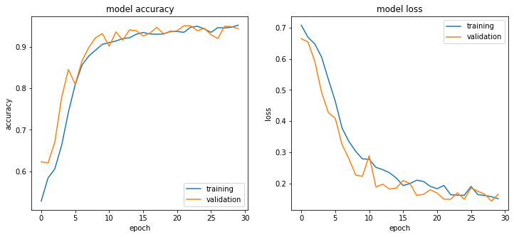
Figure 3: Evolution of the accuracy (left) and loss (right) as a function of epoch as evaluated on the training and validation samples.

3 Machine Learning Approach

Construction, training, and testing of the CNN-based ML model used in this paper were all done using the Tensorflow and Keras machine learning frameworks [13, 14].

3.1 Model Architecture

The choice of network architecture used in this work was guided by our ultimate goal of investigating whether ML techniques were feasible for detecting ghosts/scattered light artifacts, and if so, how they would compare with the conventional technique based on ray tracing. Since the main objective was a proof-of-concept demonstration, we opted for a relatively simple CNN architecture that: (1) was straightforward to implement in a common ML framework, (2) did not require significant computing resources to train, and (3) had good performance on standard image classification data sets that would carry over to artifact detection in DES exposures. The CNN architecture we settled on was very similar to AlexNet [15], in its use of stacked 2D convolutional layers with rectified linear unit (ReLU) activation functions that alternate with max-pooling layers, and eventually terminated in fully connected layers with SoftMax outputs. It differed from AlexNet in terms of hyperparameters, such as the number of hidden layers, the number of kernels and their sizes, stride lengths, and dropout values.

The detailed design of the CNN we used is shown in Figure 2. The network is composed of four 2D convolutional layers, each followed by a maximum pooling layer [9, 15]. The number of output filters in the sequence of four convolutional layers are 16, 32, 32, and 64, respectively. Filters in all four convolutional layers have kernel sizes of $3\times 3$, stride lengths of one, and use ReLU activation functions. The pool sizes used in the pooling layers are $4\times 4$ for the first layer and $2\times 2$ for all subsequent layers. Stride lengths for all pooling layers correspond to their pool sizes. The final two layers of the network, following the fourth pooling layer, are fully connected (FC) layers. The first FC layer has 128 neurons with ReLU activation functions and the last FC layer has 2 output neurons using SoftMax activation functions. The larger of these two outputs, which sum to a value of one, was selected to determine the model prediction. “Dropouts” are performed prior to each FC layer in which a fraction (0.4 and 0.8 for the first and second FC layers, respectively) of the inputs are randomly ignored. This method lessens the chances of overfitting by minimizing co-adaptations between layers that do not generalize well to unseen data [16]. The total number of parameters in the model is 1,212,578.

3.2 Training the Model

The images used for training the model were derived from $800\times 723$ pixel, 8-bit grayscale images in the portable network graphics format, covering the full DECam focal plane. These images were produced with the STIFF program [17], assuming a power-law intensity transfer curve with index $\gamma=2.2$. Minimum and maximum intensity values were set to the 0.005 and 0.98 percentiles of the pixel value distribution, respectively. The training set consisted, initially, of equal portions of images that had ghosts/scattered light (positives) and images that did not (negatives). The positive sample consisted of 2,389 images that the ray-tracing program identified as likely to have ghosts/scattered light artifacts and was drawn from the full set of $\sim$132k images from all DES observing periods. After excluding the images flagged by ray-tracing program, an equal number of images were randomly selected from the remainder of the full data set to form the negative sample of the training set.

Prior to feeding the images to the network, they were first downsampled to $400\times 400$ pixels, which is the input size of the first convolutional layer. The pixel values in each image were then normalized to a range whose minimum and maximum corresponded, respectively, to the first quartile $Q_{1}(x)$ and third quartile $Q_{3}(x)$ of the full distribution in the image, by multiplying each pixel value, $x_{i}$, by a factor $s_{i}=\frac{x_{i}-Q_{1}(x)}{Q_{3}(x)-Q_{1}(x)}$. To improve the model’s ability to correctly identify images that contain ghosts/scattered light artifacts, the training images were also randomly flipped either along the horizontal axis by reversing the ordering of pixel rows, or along the vertical axes by reversing the ordering of pixel columns. This was done using the ImageDataGenerator class in Keras, which does an in-place substitution of the input images with the flipped versions, without changing the total size of the data sample [14].

3.2.1 Model Training Procedure

The model was trained using 80% of the sample described in the previous section and the remaining fraction was set aside for validation. Apart from this training/validation sample was a separate test sample used to evaluate the model, which is described in Section 3.3. Optimal weights for the model were obtained using Adam [18], a version of the mini-batch stochastic gradient method that uses dedicated learning rates for each parameter and adapts their values based on their history. The weights were updated iteratively in randomly picked batches of 32 images (batch size), completing a full pass over the entire sample in one epoch. A total of 30 training epochs were performed. The loss function used was categorical cross-entropy, calculated according to $L=-\sum_{i=1}^{N}\sum_{j=1}^{M}y_{ij}\cdot log(p_{ij})$, where the index $i$ runs over the number of observations, $N$, and the index $j$ is taken over the number of classes, $M$. $p_{ij}$ is the probability and $y_{ij}$ is either 0 or 1, depending on whether class $j$ is the correct classification for observation $i$. In our case, we have two classes ($M=2$) corresponding to whether or not an image contains a ghost/scattered light artifact.

Upon visual examination of the false positives and false negatives after training, it was found that some images were mislabeled. This was because images labeled as lacking ghosts/scattered light artifacts were initially selected based on the ray-tracing program output. As it turned out, many “clean” images actually contained ghosts/scattered light. When images that were positively identified by the ray-tracing program were inspected, the opposite case was also found to be true – some images labeled as having ghosts/scattered light did not exhibit detectable artifacts. Therefore, several iterations were required in order to fix the mislabeled images and repeat the 30-epoch training process.

3.2.2 Training and Validation Results

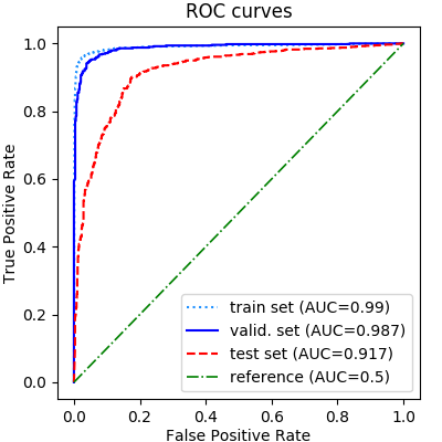
Figure 4: ROC curves and the associated areas under the ROC curves (AUCs) are shown separately for the training, validation, and independent test samples. The green dash-dotted line represents the reference case of no discriminating power (AUC=0.5).

The final results of training are shown in Figures 3, 4, and 5. The two panels in Figure 3 show the evolution of the training accuracy (left) and loss (right) over the epochs. The validation curves follow the training curves closely, indicating no overfitting. Accuracies of over 94% are achieved on both training and validation sets at the end of 30 epochs.

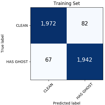
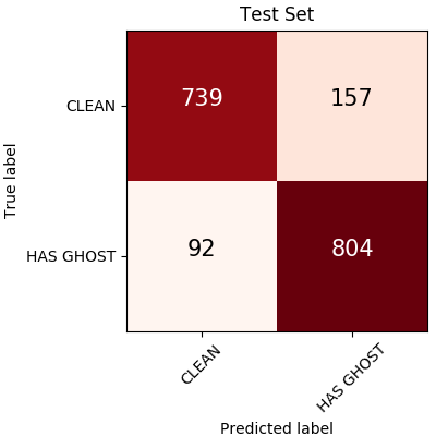
(a)	(b)	(c)

Figure 5: The confusion matrices are shown separately for the (a) training, (b) validation, and (c) independent test samples. In each matrix, the number of true negatives and positives are shown, respectively, in the upper left and right boxes, while the number of false positives and negatives are shown, respectively, in the upper right and lower left boxes.

Performance Summary
Sample	Accuracy	Precision	Recall	AUC
training	0.963	0.959	0.967	0.990
validation	0.944	0.927	0.959	0.987
test	0.861	0.837	0.897	0.917

Table 1: Summary of performance metrics for each sample. Accuracy, precision, and recall are calculated as described in Section 3.3 using the values in Figure 5. The AUCs are the areas under the ROC curves in Figure 4.

Figure 4 plots the receiver operating characteristic curve (ROC) for the trained model, showing the true postive rate versus the false positive rate. The curves resulting from the application of this model to the training (light blue dotted line) and validation (solid blue line) samples are shown separately. The area under the ROC curve (AUC) for the validation sample is 0.987, indicating good separation between the two classes of images. For comparison, the diagonal green dash-dotted line shows the case when a model has absolutely no discriminating power between classes where AUC=0.5.

Figures 5a and 5b plot the confusion matrices for the training and validation samples, respectively. In each matrix, the values in the first row represent the number of true negatives in the first column and the number of false positives in the second column. The values in the second row represent the number of false negatives in the first column and the number of true positives in the second column.

3.3 Evaluating the Model

The validation set was not used directly to train the model, however, it served as an early indicator of model performance in the training process. In this respect, it could have influenced the model and hyperparameter choices. The performance of the fully trained model was therefore evaluated in an unbiased way using an independent test data sample. This sample was constructed by visually selecting an equal number of images containing ghosts/scattered light artifacts and those without them, and labeling them according to their true class. It consisted of 1,761 DECam images spread across all DES data taking periods. It also excluded all the images used for training and validation, and was $\sim$37% of that sample in size. The fully trained model was applied to this sample to predict which class they belonged to. The ROC curve for the test data sample is represented by the dashed red line in Figure 4 with AUC=0.917, indicating good discrimination between the two classes. From the confusion matrix shown in Figure 5c, one calculates $accuracy=\mathrm{\frac{TP+TN}{Total}}=0.861$, $precision=p=\mathrm{\frac{TP}{TP+FP}}=0.837$, $recall=r=\mathrm{\frac{TP}{TP+FN}}=0.897$, and $F_{1}=2\cdot\frac{p\cdot r}{p+r}=0.866$, where TP, FP, TN, and FN are, respectively, the number of true positives, false positives, true negatives and false negatives. These results are summarized in Table 1 together with those for the training and validation samples.

Typical examples of misclassified images from the test sample, in the form of false positives and false negatives, are shown in Figures 6 and 7, respectively. Although the images in the first class of false positives represented by Figures 6a–6c do not bear an obvious resemblance to those containing ghosting/scattered light artifacts, they all exhibit poor data quality from nearly a magnitude of extinction due to clouds that may be confusing the CNN. These images do not pass the high-level DES data quality criteria. The second class of false positives contain objects that exhibit features similar to those found in ghosting artifacts (Figures 6d–6f) and scattered light artifacts (Figures 6g & 6h), making them intuitively easier to appreciate. The third class of false positives, represented by Figure 6i, are in some sense true positives, because they contain faint artifacts close to the human detection threshold. In this image, there is a ghost artifact faintly visible in the 4th and 5th columns from the left, in the two middle rows of CCDs. The false negatives in Figure 7 are easier to understand because they all contain ghost artifacts that are not too difficult to see (their locations are described in the figure caption).

Our application involves a large data set where images with ghosts/scattered light constitute a relatively small fraction of the entire sample. False negatives carry a high cost due to their detrimental effects on astronomical measurement and the difficulty of manual identification in a data set of this size. On the other hand, false positives are less of a problem since they are easier to identify from the smaller sample predicted by the model to be ghosts/scattered light. Our model’s true positive rate or $recall$ of $\sim$90% shows it is able to identify a significant fraction of all images with ghosts/scattered light, and its $precision$ of $\sim$84% indicates that false positives are also kept under control, both of which are favorable characteristics for this application. As indicated by the AUC, our model performs better on the training and validation set than on the test set. This may be an indication of biases introduced in the construction of the former set, which is based on images identified by the ray-tracing program.

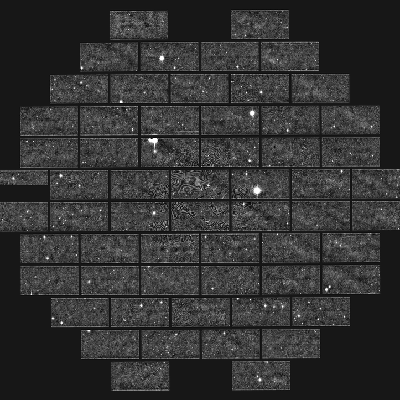
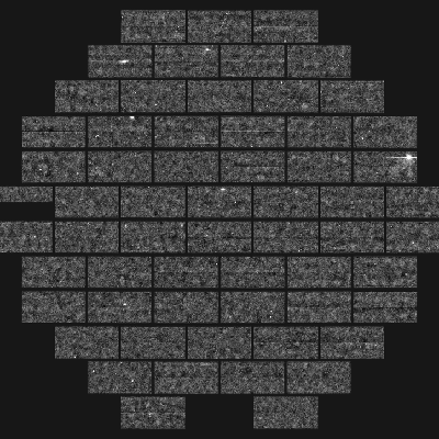
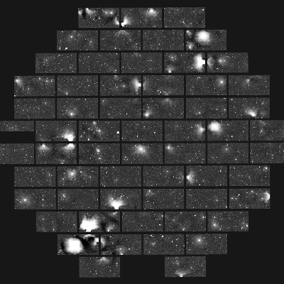
(a)	(b)	(c)
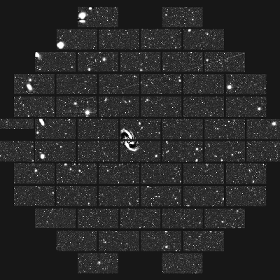
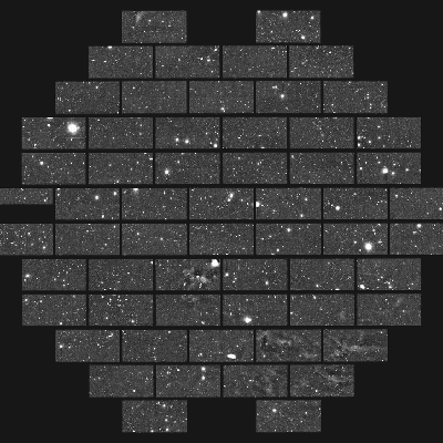
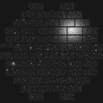
(d)	(e)	(f)
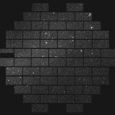
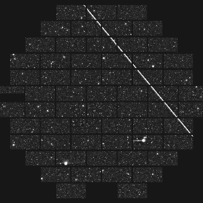
(g)	(h)	(i)

Figure 6: Example false positives found by the trained model in the test set described in Section 3.3. The exposures shown in panels (a), (b), and (c) have poor data quality due to heavy cloud cover which contributes to misclassification by the CNN. The barred spiral NGC 1365 in the Fornax galaxy cluster (d), Galactic cirrus (e), and the Omega Centauri globular cluster in (f), exhibit features similar to those found in ghosting artifacts. The faint resolved stars in the periphery of the LMC in (g), and the artificial earth-orbiting satellite track in (h), have features found in scattered light artifacts. There is a barely visible ghost artifact in columns 4 & 5 of the middle two rows of CCDs in (i).

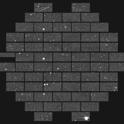
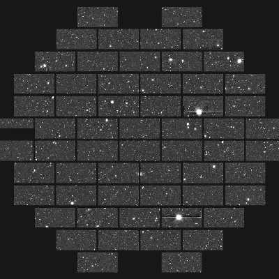
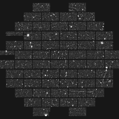
(a)	(b)	(c)

Figure 7: Selected examples of false negatives found by the trained model in the test set described in 3.3. Faint ghosts/scattered light artifacts are visible in the upper left corner of (a), rightmost column CCD in the 5th row from the top of (b), and rightmost column CCDs in the 8th and 9th rows from the top of (c).

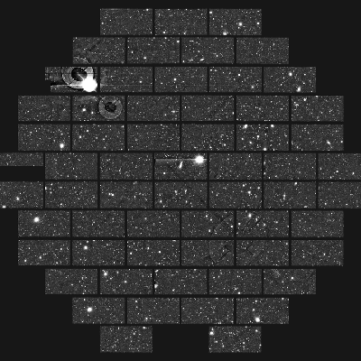
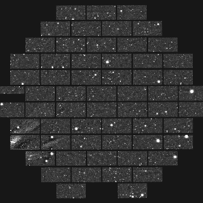
(a)	(b)
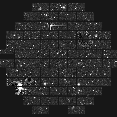
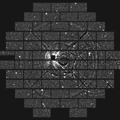
(c)	(d)
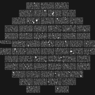
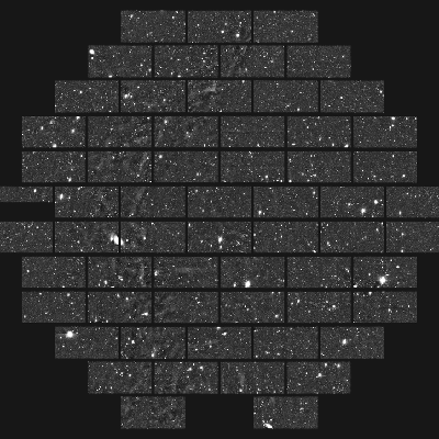
(e)	(f)

Figure 8: The images above are examples of DES Year 5 images predicted by the CNN described in this paper to exhibit ghosts/scattered light artifacts, but which were not identified by the ray-tracing algorithm as such. Figures (a) to (d) show examples that have actual artifacts, representing true positives. Figures (e) and (f) are examples of the $\sim$23% described in the text that either do not exhibit artifacts or have negligible levels, representing false positives.

4 Applying the Trained Model on DES Data and Comparing with the Traditional Method

The CNN trained according to the details described in Section 3.2 was used to perform inference on the DES Year-5 data set consisting of 23,755 full focal plane DECam images with exposure numbers ranging from 666747 to 724364, which were prepared using the procedure described in Section 3.2. This set also included the Year-5 images that were used in the training+validation and testing stages. For each image, the model was used to predict whether it contained ghosts/scattered light or whether it was free from such artifacts. The model identified 3,285 images as positives, containing ghosts/scattered light artifacts. Several examples of these images are shown in Figure 8. Only 716 images in this set of positives were false positives, exhibiting nearly imperceptible or no sign of ghosts/scattered light artifacts. The precision achieved was therefore $p=\nicefrac{{2569}}{{3285}}=0.782$.

For comparison, the ray-tracing program described in Section 2 classified 259 DES Year-5 images as containing artifacts. Out of these, 241 were in common with the set of positives identified by the ML model, and all of the images in this overlap region were true positives. The remaining 18 that were positively classified only by the ray-tracing program were all true positives except for 8. The precision achieved by the ray tracing model was therefore $p=\frac{{241+10}}{259}=0.969$.

The difference in precision from the two methods may be due to the more limited range of image types dealt with by the ray-tracing program, and the issue raised in Section 3.3 about the training and validation set being based on the images identified by that program.

5 Computer Resource Utilization

The conventional ray tracing algorithm takes on the order of a few ms per image for actual ray tracing. Additional time is spent querying the bright star catalog around each exposure as a pre-processing step. This algorithm was run on a yearly basis as input to the DES data processing.

For the CNN-based approach, training the model over 30 epochs using the procedure described in Section 3.2.1 on a laptop with an Intel Xeon E-2176M CPU, 32GB RAM, and a mid-range 4GB Nvidia Quadro P2000 Mobile GPU took 8.8 min (18 s/epoch) to complete. Utilizing the 16GB Nvidia P100 GPUs available in the Google Cloud Colaboratory Jupyter notebook environment [19], reduces the training time by a factor of $4\times$ (4.4 s/epoch).

The process of performing inference with the CNN on the 23,755 image DES Year-5 data set described in Section 4 took 50 s (2 ms/image) on the Quadro-equipped laptop described above. Such short inference times are indeed promising for real-time artifact identification on future large-scale cosmic surveys, especially since the network model has not even been optimized for speed yet. Furthermore, there now exist practical high-level synthesis tools that can implement these network models on FPGA hardware for critical real-time applications [20].

6 Conclusion

We have successfully applied a machine learning based method to identify DES images containing ghosts/scattered light artifacts. This method positively identified $\sim$97% of all images that had been previously identified as containing artifacts by a traditional ray-tracing method. Overall, it also identified $\sim$10$\times$ more images with actual artifacts, with a precision of $\sim$78%. This serves as a proof-of-principle demonstrating the effectiveness of using modern ML methods in identifying ghosts/scattered light in optical telescope images from a cosmic survey. It lays the foundation for possible future refinements. The scope of this work was limited to detecting the presence of these artifacts in an image without identifying their location within the image. In future work, we will take advantage of recent developments in object detection and semantic segmentation to expand the capability of our method to include the identification of the individual pixels associated with each artifact [21]. Such enhancements, coupled with the results presented in this work, will benefit future cosmic surveys like the LSST, which will be faced with the challenge of even larger data sets.

7 Acknowledgements

This collaborative work was carried out as part of an Illinois Mathematics and Science Academy (IMSA) Student Inquiry and Research (SIR) project. We wish to thank Dr. Don Dosch, Dr. David Devol, and Dr. Eric Smith of IMSA for overseeing the SIR program and making this collaboration possible. We also wish to thank the staffs of Fermilab’s experimental astrophysics group and IMSA’s SIR office for their support.

Funding for the DES Projects has been provided by the U.S. Department of Energy, the U.S. National Science Foundation, the Ministry of Science and Education of Spain, the Science and Technology Facilities Council of the United Kingdom, the Higher Education Funding Council for England, the National Center for Supercomputing Applications at the University of Illinois at Urbana-Champaign, the Kavli Institute of Cosmological Physics at the University of Chicago, the Center for Cosmology and Astro-Particle Physics at the Ohio State University, the Mitchell Institute for Fundamental Physics and Astronomy at Texas A&M University, Financiadora de Estudos e Projetos, Fundação Carlos Chagas Filho de Amparo à Pesquisa do Estado do Rio de Janeiro, Conselho Nacional de Desenvolvimento Científico e Tecnológico and the Ministério da Ciência, Tecnologia e Inovação, the Deutsche Forschungsgemeinschaft and the Collaborating Institutions in the Dark Energy Survey.

The Collaborating Institutions are Argonne National Laboratory, the University of California at Santa Cruz, the University of Cambridge, Centro de Investigaciones Energéticas, Medioambientales y Tecnológicas-Madrid, the University of Chicago, University College London, the DES-Brazil Consortium, the University of Edinburgh, the Eidgenössische Technische Hochschule (ETH) Zürich, Fermi National Accelerator Laboratory, the University of Illinois at Urbana-Champaign, the Institut de Ciències de l’Espai (IEEC/CSIC), the Institut de Física d’Altes Energies, Lawrence Berkeley National Laboratory, the Ludwig-Maximilians Universität München and the associated Excellence Cluster Universe, the University of Michigan, the National Optical Astronomy Observatory, the University of Nottingham, The Ohio State University, the University of Pennsylvania, the University of Portsmouth, SLAC National Accelerator Laboratory, Stanford University, the University of Sussex, Texas A&M University, and the OzDES Membership Consortium.

Based in part on observations at Cerro Tololo Inter-American Observatory, National Optical Astronomy Observatory, which is operated by the Association of Universities for Research in Astronomy (AURA) under a cooperative agreement with the National Science Foundation.

The DES data management system is supported by the National Science Foundation under Grant Numbers AST-1138766 and AST-1536171. The DES participants from Spanish institutions are partially supported by MINECO under grants AYA2015-71825, ESP2015-66861, FPA2015-68048, SEV-2016-0588, SEV-2016-0597, and MDM-2015-0509, some of which include ERDF funds from the European Union. IFAE is partially funded by the CERCA program of the Generalitat de Catalunya. Research leading to these results has received funding from the European Research Council under the European Union’s Seventh Framework Program (FP7/2007-2013) including ERC grant agreements 240672, 291329, and 306478. We acknowledge support from the Brazilian Instituto Nacional de Ciência e Tecnologia (INCT) e-Universe (CNPq grant 465376/2014-2).

This manuscript has been authored by Fermi Research Alliance, LLC under Contract No. DE-AC02-07CH11359 with the U.S. Department of Energy, Office of Science, Office of High Energy Physics.

8 Contributions

The author list is ordered alphabetically. C. Chang was responsible for the initial idea of applying ML techniques to artifact detection and served as primary mentor to D.M. Wang in the SIR project. A. Drlica-Wagner identified optical ghosts/scattered light detection as an important problem that could benefit from an alternative approach. He also ran the ray-tracing algorithm, provided access to labeled images containing ghosts/scattered light, and advised on their classification and causes. S. Kent developed the DECam ray-tracing algorithm and provided expertise on the origins of ghosts and scattered light in the DECam system. B. Nord provided initial training on ML algorithms and advised on algorithm design. He also served as the primary liason between the astrophysics group at Fermilab and IMSA. D.M. Wang was responsible for extending the sample ML models provided by B. Nord to develop the models used in this work. She also performed the training and validation of the model, including selecting its set of hyperparameters. M.H.L.S. Wang prepared the samples used for training and comparisons, based on the data A. Drlica-Wagner provided access to. He also advised on the preprocessing of the data and prepared the initial version of this document, including the model architecture diagram.

References

- [1] DES Collaboration, The Dark Energy Survey (2005). arXiv:astro-ph/0510346.
- [2] DES Collaboration, The Dark Energy Survey: more than dark energy – an overview, MNRAS 460 (2) (2016) 1270–1299. doi:10.1093/mnras/stw641.
- [3] B. Flaugher, et al., The Dark Energy Camera, Astron. J. 150 (2015) 150. arXiv:1504.02900, doi:10.1088/0004-6256/150/5/150.
- [4] S. M. Kent, Ghost Images in DECam, FERMILAB-SLIDES-20-114-SCD (2013). doi:10.2172/1690257.
- [5] D. Tanoglidis, et al., Shadows in the Dark: Low-Surface-Brightness Galaxies Discovered in the Dark Energy Survey (2020). arXiv:2006.04294.
- [6] v. Z. Ivezić, et al., LSST: from Science Drivers to Reference Design and Anticipated Data Products, Astrophys. J. 873 (2) (2019) 111. arXiv:0805.2366, doi:10.3847/1538-4357/ab042c.
- [7] A. L. Samuel, Some studies in machine learning using the game of checkers, IBM Journal of Research and Development 3 (3) (1959) 210–229. doi:10.1147/rd.33.0210.
- [8] D. H. Hubel, T. N. Wiesel, Receptive fields of single neurones in the cat’s striate cortex, The Journal of Physiology 148 (3) (1959) 574–591. doi:10.1113/jphysiol.1959.sp006308.
- [9] Y. Lecun, L. Bottou, Y. Bengio, P. Haffner, Gradient-based learning applied to document recognition, Proceedings of the IEEE 86 (11) (1998) 2278–2324. doi:10.1109/5.726791.
- [10] G. E. Hinton, S. Osindero, Y.-W. Teh, A fast learning algorithm for deep belief nets, Neural Computation 18 (7) (2006) 1527–1554, pMID: 16764513. doi:10.1162/neco.2006.18.7.1527.
-
[11]
J. W. DeRose, W. R. Morningstar,
Automated image
artifact identification in dark energy survey ccd exposures, CS229 Final
Project Report, Stanford University (December 2015).
URL http://cs229.stanford.edu/proj2015/149_report.pdf -
[12]
K. Zhang, J. S. Bloom,
deepCR: Cosmic ray
rejection with deep learning, The Astrophysical Journal 889 (1) (2020) 24.
doi:10.3847/1538-4357/ab3fa6.
URL https://doi.org/10.3847%2F1538-4357%2Fab3fa6 -
[13]
M. Abadi, et al., TensorFlow: Large-scale
machine learning on heterogeneous systems, software available from
tensorflow.org (2015).
URL https://www.tensorflow.org/ - [14] F. Chollet, et al., Keras, https://keras.io (2015).
- [15] A. Krizhevsky, I. Sutskever, G. E. Hinton, Imagenet classification with deep convolutional neural networks, in: F. Pereira, C. J. C. Burges, L. Bottou, K. Q. Weinberger (Eds.), Advances in Neural Information Processing Systems 25, Curran Associates, Inc., 2012, pp. 1097–1105.
-
[16]
N. Srivastava, G. Hinton, A. Krizhevsky, I. Sutskever, R. Salakhutdinov,
Dropout: A simple way to
prevent neural networks from overfitting, Journal of Machine Learning
Research 15 (2014) 1929–1958.
URL http://jmlr.org/papers/v15/srivastava14a.html - [17] E. Bertin, Displaying Digital Deep Sky Images, in: P. Ballester, D. Egret, N. P. F. Lorente (Eds.), Astronomical Data Analysis Software and Systems XXI, Vol. 461 of Astronomical Society of the Pacific Conference Series, 2012, p. 263.
-
[18]
D. P. Kingma, J. Ba, Adam: A method for
stochastic optimization, in: 3rd International Conference on Learning
Representations, ICLR 2015, San Diego, CA, USA, May 7-9, 2015, Conference
Track Proceedings, 2015.
URL http://arxiv.org/abs/1412.6980 - [19] Google LLC, Colaboratory: Frequently asked questions, https://research.google.com/colaboratory/faq.html (2021).
- [20] J. Duarte, et al., Fast inference of deep neural networks in FPGAs for particle physics, JINST 13 (07) (2018) P07027. arXiv:1804.06913, doi:10.1088/1748-0221/13/07/P07027.
- [21] K. He, G. Gkioxari, P. Dollár, R. Girshick, Mask r-cnn (2018). arXiv:1703.06870.