$f(R)$ Dual Theories of Quintessence : Expansion-Collapse Duality

Abstract

The accelerated expansion of the universe demands presence of an exotic matter, namely the dark energy. Though the cosmological constant fits this role very well, a scalar field minimally coupled to gravity, or quintessence, can also be considered as a viable alternative for the cosmological constant. We study $f(R)$ gravity models which can lead to an effective description of dark energy implemented by quintessence fields in Einstein gravity, using the Einstein frame-Jordan frame duality. For a family of viable quintessence models, the reconstruction of the $f(R)$ function in the Jordan frame consists of two parts. We first obtain a perturbative solution of $f(R)$ in the Jordan frame, applicable near the present epoch. Second, we obtain an asymptotic solution for $f(R)$, consistent with the late time limit of the Einstein frame if the quintessence field drives the universe. We show that for certain class of viable quintessence models, the Jordan frame universe grows to a maximum finite size, after which it begins to collapse back. Thus, there is a possibility that in the late time limit where the Einstein frame universe continues to expand, the Jordan frame universe collapses. The condition for this expansion-collapse duality is then generalized to time varying equations of state models, taking into account the presence of non-relativistic matter or any other component in the Einstein frame universe. This mapping between an expanding geometry and a collapsing geometry at the field equation level may have interesting potential implications on the growth of perturbations therein at late times.

1 Introduction

Observational evidence shows that currently the universe is going through a phase of accelerated expansion [1, 2]. This observation necessitates the existence of an exotic fluid that violates the ‘Strong Energy Condition’ [3, 4, 5], referred to as the dark energy (DE) [6, 7, 8]. The cosmological constant ($\Lambda$) model is the simplest implementation of dark energy in Einstein’s general theory of relativity [9, 10, 7]. The $\Lambda$CDM ($\Lambda$ plus Cold Dark Matter) model is also consistent with observations [11, 12, 13, 14, 15, 16], it is in fact the simplest and most widely used model to describe dark energy. The energy density contributed by $\Lambda$ is conventionally associated with the energy density of vacuum. From a theoretical point of view, the Lagrangian for the cosmological constant model, i.e., the Einstein-Hilbert action with an added constant ($\mathcal{L}\sim\sqrt{-g}(R-2\Lambda)$), has somewhat a unique status, as in $1+3$ dimensional spacetime it is arguably the simplest generally covariant Lagrangian, that leads to second order equations of motion [17, 18]. The energy density corresponding to $\Lambda$ does not vary with the scale factor of the universe and the equation of state parameter ($w=P/\rho$, where $P,\rho$ are pressure and energy density respectively) associated with $\Lambda$ is precisely a constant, $w_{\Lambda}=-1$. Although $w_{\text{DE}}=-1$ is consistent with observations, deviation from this value is not completely ruled out. Apart from this, the cosmological constant model suffers from the fine tuning problem  [10, 7, 9]. For example, a naive estimate of the vacuum energy density of quantum fields, integrated up to the Planck length cut off, can be given as $\rho_{\text{vacuum}}\sim\hbar k_{\text{Planck}}^{4}\sim 10^{74}\text{GeV}^{4}$, whereas, observations predict the energy density of the cosmological constant to be $\rho_{\Lambda}\sim 10^{-47}\text{GeV}^{4}$, which has a huge discrepancy of the order of $121$ with the theoretical estimate. This discrepancy can only be rectified by fine tuning $\rho_{\text{vacuum}}$, which is one of the shortcomings of the $\Lambda$CDM model [10, 7, 9]. It has also been pointed out that a higher value of the $\Lambda$ would make dark energy take over the matter energy density ($\rho_{\text{m}}$) at an early epoch. If this would have happened at a sufficiently early time, the accelerating expansion could have prevented the possibility of structure formations in the universe. The cosmological constant is needed to be fine tuned even in the very early universe, such that the dark energy-matter equality ($\rho_{\Lambda}/\rho_{\text{m}}\sim\mathcal{O}(1)$) occurs during the current epoch.

To overcome these problems with the cosmological constant, several dynamical models of dark energy have been proposed. Unlike the cosmological constant model, a time-dependent model of dark energy can be fitted with the observations from the current accelerating phase, where it really makes the impact. A scalar field minimally coupled to gravity, or quintessence, was introduced to provide a simple dynamical description of dark energy (see, for example, [19, 20, 21, 22, 23, 24, 25, 26, 27, 28, 29, 30, 31]). The potential ($V$) of the quintessence field ($\varphi$) can be set up to be sufficiently flat during the current epoch, such that the kinetic term of the field becomes negligible ($\partial_{\mu}\varphi\sim 0$). This makes the equation of state parameter of the field, $w_{\varphi}\to-1$, hence the quintessence field mimics the cosmological constant model at the current epoch (see [6, 7, 8] and their references for detailed review).

There is also the possibility that an explanation for dark energy might arise from the outside of Einstein’s gravity framework. A simple form of such extended gravity theories is $f(R)$ gravity, where instead of Ricci scalar $R$, a general function of the curvature scalar, $f(R)$, is used in the Einstein-Hilbert action (see, for example, [32, 33, 34, 35, 36, 37, 38, 39, 32, 40, 41] and references therein for recent works in $f(R)$ gravity, for reviews see [42, 43, 44]). There are roughly two approaches one can take to describe dark energy vis-a-vis $f(R)$ gravity.

The first approach is to treat modified gravity as a ‘correction’ to Einstein’s gravity, such that the ‘correction’ itself is responsible for the acceleration of the universe. Here it is convenient to treat the deviation of the Einstein field equation from the modified field equation as an effective energy momentum tensor of a perfect fluid. One of the early examples of this approach can be found in [45] in the context of inflation. Later it was extensively studied in the context of late-time acceleration as well (for example, see [46, 47, 48, 49]). The cosmological viability of $f(R)$ in such models was discussed in [50, 42, 43].

There is also another approach where the dark energy implemented by a quintessence field (in Einstein gravity) can effectively be studied as a pure gravity theory governed by an $f(R)$ action. It is well known that a conformal transformation of the metric of the $f(R)$ action can lead to a theory of Einstein’s gravity with a quintessence field, in a conformally connected spacetime (see, for example, [51, 52, 53, 54, 55, 56, 57, 43, 42, 58, 59, 60, 61, 62, 63]). The description of the universe, where the gravity action becomes Einstein-Hilbert action, is referred to as the ‘Einstein frame’, whereas, the initial description is referred to as the ‘Jordan frame’.

The conformal parameter of this transformation is given by the $f(R)$ model itself. This establishes a duality between $f(R)$ gravity without quintessence field in Jordan frame and Einstein gravity with quintessence field in Einstein frame, such that, an $f(R)$ function corresponds to a quintessence potential. Due to this duality, one can treat a quintessence model in Einstein gravity as an $f(R)$ gravity model, without the need of a quintessence field.

In this paper, we are interested mainly in quintessence models with an equation of state $w(a)=w_{0}-w^{\prime}\ln a$. The corresponding quintessence potential has a closed and relatively simple analytical form. This parameterization was first introduced in [64] to fit with three tracking quintessence models. It was shown to be a good fit with observations in the redshift range $z\lesssim 4$. This model was further extended in [65] to account for observation from a wider range of redshift parameter. Models with logarithmic $w(a)$ were further constrained from the SNIa+BAO+H($z$) data in [66, 67]. We obtain a class of $f(R)$ theories that can recover these potentials in Einstein frame. The reconstruction of the $f(R)$ function can be broken in to two parts. For the near current time in the Einstein frame, we find perturbative solutions of $f(R)$ which are valid in the small Jordan frame curvature limit. From this we estimate the perturbative solution which is most suited in the current epoch of the Einstein frame universe. For the distant future in Einstein frame, we obtain an asymptotic solution for $f(R)$.

We further show that the logarithmic parameterization of $w(a)$ belongs to a class of quintessence models for which the Jordan frame scale factor has a finite maximum value. In the late time limit of the Einstein frame universe, the Einstein frame scale factor increases indefinitely, while the Jordan frame universe collapses after attaining a maximum. A general condition for the collapse of the Jordan frame is then obtained which takes into account other components of the universe. Using this we find that the presence of dust prevents the Jordan frame collapse. Finally, we show that the introduction of positive spatial curvature [68] may still allow the expansion-collapse duality in the presence of non-relativistic matter.

The general condition for the expansion-collapse duality of the Einstein and Jordan frame can be used in further studies to explore other viable quintessence models. An expanding universe with quintessence field can also be looked at as a collapsing universe with different equations of motion. Such a correspondence between expanding and collapsing geometries can have applications in studies of growth of cosmological perturbations. For example, one can study the back reaction of the curvature and matter perturbations in our universe collectively as a gravitational perturbation of a collapsing geometry leading to a good estimate of back reaction at late times.

The paper is organized as follows. In Sec. 2 we review the quintessence model and the reconstruction of the quintessence field potential. In Sec. 3 we obtain the analogous $f(R)$ theories consistent with the quintessence model; first perturbatively near current era and then for remote future. A relation between the scale factors of the FRW universes in the Einstein and the Jordan frame is then obtained in Sec. 4. Here we demonstrate that at late times the Jordan frame universe collapses back unlike the universe driven by the quintessence field in the Einstein frame. In Sec. 5 we derive a general condition for the expansion-collapse duality and further explore the effect of dust and spatial curvature on the collapse of the Jordan frame. We conclude the paper with a summary and discussion of implications in Sec. 6.

2 Reconstruction of quintessence field potentials

The accelerated expansion of the universe requires the presence of dark energy, characterized by an equation of state parameter $w<-1/3$, this is generally termed as violation of the ‘strong energy condition’. A scalar field minimally coupled to gravity, or quintessence, is a viable candidate for dark energy (see [7, 69, 6]). In this section we briefly review the quintessence models corresponding to constant and logarithmic equation of state parameters.

2.1 Quintessence model of dark energy

The action of a generic quintessence field in Einstein gravity is give by

$$\mathcal{S}_{Q}=\int d^{4}x\sqrt{-g}\frac{R}{2\kappa^{2}}-\int d^{4}x\sqrt{-g}\left(\frac{1}{2}\partial_{\mu}\Phi\partial^{\mu}\Phi+V(\Phi)\right).$$ (2.1)

Here $\kappa^{2}=8\pi G$, $R$ is Ricci scalar, and $g_{\mu\nu}$ is taken to be the spatially flat FRW metric,

$$g_{\mu\nu}\dot{=}\text{diag}\left(-1,a^{2}(t),a^{2}(t),a^{2}(t)\right).$$

The quintessence field $\Phi$ is taken as a function of time only. The definition of the energy-momentum tensor,

$$T_{\mu\nu}=\frac{-2}{\sqrt{-g}}\frac{\delta S_{\Phi}}{\delta g^{\mu\nu}}$$ (2.2)

leads to energy density ($\rho$) and pressure ($P$) associated with the field,

$$T_{00} =\rho=\frac{\dot{\Phi}^{2}}{2}+V$$ (2.3)

$$T^{i}_{i} =P=\frac{\dot{\Phi}^{2}}{2}-V,$$ (2.4)

where the dot represents derivative with respect to comoving time. From this one can recover the quintessence potential and the time derivative of the field as,

$$V =\frac{1}{2}(1-w(a))\rho(a),$$ (2.5)

$$\dot{\Phi}^{2}=(1+w(a))\rho(a),$$ (2.6)

leading to the equation of state parameter $w(a)$,

$$w(a)=\frac{P}{\rho}=\frac{\frac{1}{2}\dot{\Phi}^{2}-V(\Phi)}{\frac{1}{2}\dot{\Phi}^{2}+V(\Phi)}.$$ (2.7)

This shows that for a slowly rolling quintessence field, i.e., if the kinetic term of the field becomes negligible with respect to the potential ($V(\Phi)\gg\dot{\Phi}^{2}$), then $w\to-1$, therefore the quintessence field becomes capable of driving the acceleration.

For example, if the equation of state parameter ($w$) is time-independent, then the continuity equation

$$\nabla_{\mu}T^{\mu\nu} =0,$$ (2.8a)

$$\dot{\rho}+3H\rho(1+w) =0$$ (2.8b)

can be solved to obtain the energy density as $\rho(a)=\rho_{0}a^{-3(1+w)}$, where $H=\dot{a}/a$ is the Hubble parameter. Using this in (2.6), together with the Friedmann equation

$$H^{2}=\frac{\kappa^{2}}{3}\rho(a),$$ (2.9)

one can obtain the scale factor dependence of the field $\Phi$ as

$$\varphi(a)=\Phi(a)-\Phi_{0} =\sqrt{\frac{3(1+w)}{\kappa^{2}}}\ln{a},$$ (2.10)

here $\Phi_{0}$ is the value of the field at current scale factor $a=1$. In this case the reconstructed quintessence potential becomes [67]

$$V(\varphi)=\frac{1}{2}(1-w)\rho_{0}\exp\left(-\sqrt{3\kappa^{2}(1+w)}(\varphi)\right).$$ (2.11)

2.2 Quintessence with logarithmic equation of state parameter

The cosmological constant model provides a constant energy density of dark energy with $w_{\text{DE}}=-1$. In general, $w$ can take other values and can also vary with time. Time-dependence in $w$ is often introduced by postulating a functional form of $w(a)$ with adjustable parameters. These parameters of the model $w(a)$ can then be constrained from different cosmological observations. Several parameterizations of $w(a)$ have been proposed [64, 70, 71, 65, 72] (for reviews see [73, 74, 7, 66, 75]).

Given a parameterization of $w(a)$, one can, in principle, reconstruct the corresponding quintessence field potential $V(\Phi)$. In this paper we reconstruct the $f(R)$ action corresponding to the quintessence model, where the functional form of $V(\Phi)$ plays a crucial part. We consider the logarithmic parameterization of $w(a)$, which leads to a quintessence potential with a closed and relatively simple functional form; the parameterization is given by

$$w(a)=w_{0}-w^{\prime}\ln a,$$ (2.12)

where $w_{0}$ and $w^{\prime}$ are the constant parameters. This parameterization was first introduced in [64] to fit several tracking quintessence models, and it was shown to be consistent with low redshift observations. Later on a modification on this parameterization was proposed in [65] to make this model compatible in the $z\to\infty$ limit. Recently, this parameterization was constrained from SNIa+BAO+H($z$) data in [66] and the corresponding quintessence potential was reconstructed in [67]. The ranges of the quintessence parameters within $3\sigma$ confidence level, compiled from SNIa+BAO+H($z$) data is provided in [66, 67] as

$$-1.09\leq w_{0}\leq-0.66,\ -1.21\leq w^{\prime}\leq 0.25,\ 0.26\leq\Omega_{M}\leq 0.32.$$ (2.13)

One can solve the continuity equation (2.8b) for this model to obtain the energy density in terms of the scale factor as

$$\rho(a) =\rho_{0}a^{-3(1+w_{0})+\frac{3}{2}w^{\prime}\ln a},$$ (2.14)

where $\rho_{0}=\rho(a=1)$. In the limit of $a\to\infty$, the energy density becomes $0$ if $w^{\prime}<0$, and $\infty$ for $w^{\prime}>0$. The quintessence field as a function of the scale factor can be obtained as

$$\varphi(a)=\Phi(a)-\Phi_{0} =\frac{2}{\sqrt{3}}\frac{1}{\kappa w^{\prime}}\left[(1+w_{0})^{\frac{3}{2}}-{(1+w_{0}-w^{\prime}\ln a)}^{\frac{3}{2}}\right].$$ (2.15)

We note that for $w^{\prime}>0$, the field becomes complex in the limit of $a\to\infty$. In order for $\varphi$ to be real in between the current scale factor ($a_{0}=1$) and $a\to\infty$, we will exclusively consider the model with $w^{\prime}<0$. The potential of the quintessence field can be reconstructed as

$$V(\varphi) =\rho_{0}\frac{1}{2}\left[2-\left\{{(1+w_{0})}^{\frac{3}{2}}-\frac{3w^{\prime}}{2\sqrt{3}}\kappa(\varphi)\right\}^{\frac{2}{3}}\right]$$

$$\exp\left(-\frac{3}{2w^{\prime}}\left\{(1+w_{0})^{2}-\left[(1+w_{0})^{\frac{3}{2}}-\frac{3w^{\prime}}{2\sqrt{3}}\kappa(\varphi)\right]^{\frac{4}{3}}\right\}\right).$$ (2.16)

See [67] for detailed derivations of the quintessence potentials for both time-dependent and independent equation of state parameters.

3 Reconstruction of $f(R)$ models

In this section we reconstruct $f(R)$ functions in the Jordan frame which map to quintessence models discussed above, in the Einstein frame.

3.1 The Einstein frame-Jordan frame duality

$f(R)$ gravity theory is a simple extension of Einstein gravity, where the Einstein-Hilbert action is modified by replacing the Ricci scalar ($R$) with a general function of Ricci scalar $f(R)$ (see [42, 43, 59, 76] for detailed review). The action of $f(R)$ theory is given by

$$\mathcal{S}_{J} =\frac{1}{2\kappa^{2}}\int d^{4}x\sqrt{-g}f(R).$$ (3.1)

The description of the universe obtained from this action is referred to as the ‘Jordan frame’. A duality between quintessence field in Einstein gravity and $f(R)$ gravity can be established through a conformal transformation on the metric of the $f(R)$ action. The conformal transformation

$$\tilde{g}_{\mu\nu}=\Omega^{2}(x)g_{\mu\nu},$$ (3.2)

with the choice of the conformal parameter $\Omega^{2}=\partial_{R}f(R)=F(R)$, allows for the action (3.1) to be written as

$$\mathcal{S}_{E}=\int d^{4}x\sqrt{-\tilde{g}}\frac{1}{2\kappa^{2}}\tilde{R}-\int d^{4}x\sqrt{-\tilde{g}}\left[\frac{1}{2}\tilde{g}^{\mu\nu}\partial_{\mu}\varphi\partial_{\nu}\varphi+V(\varphi)\right],$$ (3.3)

where $\tilde{R}$ is the Ricci scalar corresponding to the metric $\tilde{g}_{\mu\nu}$, the scalar field $\varphi$ and the potential $V$ are identified as

$$\varphi=\frac{\sqrt{6}}{2\kappa}\ln F$$ (3.4)

and

$$V=\frac{1}{2\kappa^{2}}\frac{FR-f}{F^{2}}$$ (3.5)

(see, for example, [57, 42, 43] for more details). Universe described using the action (3.3) is referred to as the ‘Einstein frame’. The metric in the Einstein frame is taken to be a spatially flat FRW metric, i.e., $\tilde{g}_{\mu\nu}\dot{=}\text{diag}(-1,\tilde{a}^{2},\tilde{a}^{2},\tilde{a}^{2})$, where $\tilde{a}$ is the scale factor in Einstein frame.

The Einstein frame action (3.3) represents a quintessence field in Einstein gravity. The definition of the quintessence potential (3.5) is key to the duality between Einstein and Jordan frames, i.e., a quintessence potential corresponds to a $f(R)$ function in Jordan frame (see [77, 58, 78, 79, 80, 81, 82, 83], for detailed review see [44, 42, 43]). Now we will use this equivalence to constrain $f(R)$ for the quintessence potentials discussed in Sec. 2.

3.2 Time-independent equation of state parameter

We start with deriving the function $f(R)$ such that the Jordan frame becomes dual to a quintessence field with constant equation of state parameter in Einstein frame. We identify the field term in (2.10) as $\Phi-\Phi_{0}=\varphi=\sqrt{6}\ln F/(2\kappa)$. The potential (2.11) becomes

$$V =\frac{1}{2}(1-w)\rho_{0}F^{-\frac{3}{\sqrt{2}}\sqrt{1+w}}.$$ (3.6)

In order for this potential to be generated by the $f(R)$ function, (3.6) should be the same as $V$ in (3.5), i.e., $f(R)$ should satisfy the following differential equation

$$\frac{1}{2\kappa^{2}}\frac{FR-f}{F^{2}} =\frac{1}{2}(1-w)\rho{}_{0}F^{-\frac{3}{\sqrt{2}}\sqrt{1+w}},$$ (3.7a)

$$A_{1}F^{b}-FR+f =0,$$ (3.7b)

where,

$$A_{1} =\kappa^{2}\rho{}_{0}(1-w)$$ (3.8a)

$$b =-\frac{3}{\sqrt{2}}\sqrt{1+w}+2$$ (3.8b)

Equation (3.7) can be solved analytically and it has a trivial linear solution

$$f(R)=C_{1}R-A_{1}{C}_{1}^{b}$$ (3.9)

where $C_{1}$ is an integration constant. The conformal parameter in this case becomes a constant, $C_{1}$, thus we recover the cosmological constant model. The non-trivial solution of (3.7) has a power law form,

$$f(R)=\frac{b-1}{b{(A_{1}b)}^{\frac{1}{b-1}}}R^{\frac{b}{b-1}}$$ (3.10)

where $A_{1},b\neq 0$. Interestingly, this $f(R)$ model never reduces to the cosmological constant model for any finite value of the parameter $b$.

3.3 Logarithmic equation of state parameter

Now we reconstruct $f(R)$ models which lead to a scalar field potential consistent with the logarithmic equation of state parameter (2.12). In this case, it is convenient to start with a parametric solution of the $f(R)$ function.

Since $\ln F=2\kappa\varphi/\sqrt{6}$, we have

$$\diff{V} =\frac{1}{\sqrt{6}\kappa}\frac{2f-FR}{F^{2}}.$$ (3.11)

Adding (3.11) with (3.5) and rearranging the terms we get

$$f(\bar{\varphi{}}) =\exp\left(2\bar{\varphi{}}\right)\left\{2\kappa^{2}V+2\kappa^{2}\diff{V}{\bar{\varphi{}}}\right\},$$ (3.12)

where we have re-scaled the quintessence field to be dimensionless as $\bar{\varphi{}}=\ln F=2\kappa\varphi/\sqrt{6}$. Similarly, subtracting (3.11) from (3.5) and rearranging we get

$$R(\bar{\varphi{}}) =\exp\left(\bar{\varphi{}}\right)\left\{4\kappa^{2}V+2\kappa^{2}\diff{V}{\bar{\varphi{}}}\right\}.$$ (3.13)

Equations (3.12) and (3.13) represent a parametric solution for the $f(R)$ function consistent with an arbitrary quintessence potential $V(\varphi)$, where the field $\bar{\varphi{}}$ plays the role of the parameter. For the potential (2.2), equations (3.12) and (3.13) become

$$f(\bar{\varphi{}})=C\exp\left(2\bar{\varphi{}}+C_{2}\mathcal{P}^{\frac{4}{3}}\right)\left[2-\mathcal{P}^{\frac{2}{3}}+\frac{2}{3}B\mathcal{P}^{-\frac{1}{3}}-\frac{8}{3}BC_{2}\mathcal{P}^{\frac{1}{3}}+\frac{4}{3}BC_{2}\mathcal{P}\right]$$ (3.14)

and

$$R(\bar{\varphi{}})=C\exp\left(\bar{\varphi{}}+C_{2}{\mathcal{P}}^{\frac{4}{3}}\right)\left[4-2{\mathcal{P}}^{\frac{2}{3}}+\frac{2}{3}B{\mathcal{P}}^{-\frac{1}{3}}-\frac{8}{3}BC_{2}{\mathcal{P}}^{\frac{1}{3}}+\frac{4}{3}BC_{2}\mathcal{P}\right],$$ (3.15)

where we have defined the following constants

$${(1+w_{0})}^{2}=C_{1},\ \frac{3}{2w^{\prime}}=C_{2},\ {(1+w_{0})}^{\frac{3}{2}}=A,\ \frac{3\sqrt{2}}{4}w^{\prime}=B,\ C^{\prime}=\rho_{0}e^{-C_{1}C_{2}},C=\kappa^{2}C^{\prime}$$ (3.16)

and $\mathcal{P}=A-B\ln F=A-B\bar{\varphi{}}$.

3.3.1 Perturbative solution for $F(R)$

We use an analytical approximation to invert equation (3.15) to obtain $F(R)$. Specifically, we consider the $f(R)$ theory to be a small deviation from the Einstein gravity, such that, the limit $R\to 0$ recovers the Einstein gravity. We assume that the $f(R)$ function has a form

$$f(R)=R+\epsilon\psi(R),$$ (3.17)

$\epsilon$ is a constant parameter such that $|\epsilon\psi(R)/R|\ll 1$. As $R\to 0$, $f(R)$ theories are often subjected to the following two stability criteria [42, 43, 47, 84]

$$f^{\prime} =F>0$$ (3.18a)

$$f^{\prime\prime} =F^{\prime}>0.$$ (3.18b)

In an effective fluid description of $f(R)$ gravity, the contribution from the $f(R)$ action in the field equation is treated as an energy-momentum tensor of an effective fluid (reviews can be found in [42, 43]). Within this description, the term $\kappa^{2}/F$ appears as the effective gravitational coupling term. Thus, the first condition $F>0$ is required to ensure an overall positive gravitational coupling. On the other hand, when the $f(R)$ model is taken to be a dual description of a quintessence model, as in the current study, $F>0$ is necessary for the quintessence field to be real (see (3.4)). The second condition $F^{\prime}>0$ is to avoid the Dolgov-Kawasaki or matter instability [84, 47]. Taking into account the form of $f(R)$ from (3.17) and considering weak gravity regime, the metric and Ricci scalar can be perturbed as

$$g_{\mu\nu} =\eta_{\mu\nu}+h_{\mu\nu},$$ (3.19a)

$$R =0+\delta R,$$ (3.19b)

where $\eta_{\mu\nu}$ is the Minkowski metric, Ricci scalar is perturbed over the background value $0$. It can be shown that the field equation of $\delta R$ (up to first order in $\delta R$) has an effective mass-square term $\sim(3\varepsilon\psi^{\prime\prime})^{-1}$, the sign of which is determined by $F^{\prime}$ using (3.17) (see [43, 84] for the derivation). Hence, it is argued that the Ricci scalar perturbation $\delta R$ is stable only for $\psi^{\prime\prime}>0$ or $F^{\prime}>0$.

Before using the ansatz (3.17) in the current model, we first check how such perturbative solution can lead to a relation between the perturbation in the quintessence field in the Einstein frame and Ricci scalar perturbation in the Jordan frame. By considering a matter-less Jordan frame universe in the weak gravity limit, as in (3.19), and using the Einstein-Jordan frame correspondence, $2\kappa\varphi=\sqrt{6}\ln F$, one can obtain the perturbation in the quintessence field as

$$\kappa\delta\varphi=\frac{\sqrt{6}}{2}\left.\frac{F^{\prime}}{F}\right|_{R=0}\delta R=\frac{\sqrt{6}}{2}\left.\frac{\epsilon\psi^{\prime\prime}}{1+\epsilon\psi^{\prime}}\right|_{R=0}\delta R,$$ (3.20)

where the prime denotes derivative with respect to $R$. Under this assumption, the scalar field perturbation $\delta\varphi$ becomes proportional to the Ricci perturbation in the Jordan frame, $\delta R$. This relation may reveal interesting duality between the different fields in Einstein and Jordan frames.

With this motivation, we now seek a class of functions $f(R)$ for which $F(R)$ can be expanded in the powers of $R$, consistent with the current quintessence model. In order to derive an appropriate analytical form, we truncate the expansion of $F(R)$ after the quadratic term, i.e.,

$$F(R)\approx F_{A}(R)=\epsilon_{0}+\epsilon_{1}R+\epsilon_{2}R^{2}.$$ (3.21)

Here dimensions of the constants $\epsilon_{0},\epsilon_{1},\epsilon_{2}$ are such that $F(R)$ is dimensionless. The above ansatz is valid only within a region of time where $R$ is sufficiently small, such that the contributions of higher order terms of $R$ in $F(R)$ can be neglected.

The validity of the ansatz also depends upon the implicit assumption that $F(R)$ is finite valued in the region where the solution is applicable. The function $F(R)$ has to be consistent with the Einstein-Jordan frame correspondence, i.e., $F=\exp(2\kappa\varphi/\sqrt{6})$. It is possible that at some later time in the Einstein frame the field $\varphi$, and thus $F$, becomes divergent, however, the Jordan frame curvature $R$ remains finite. This is clearly in conflict with (3.21), thus the ansatz becomes invalid in such limits. It is shown later that this is exactly the case in the late time limit of Einstein frame, in that case we obtain a non-perturbative asymptotic solution.

We obtain the perturbative solution for $F(R)$ by deriving the coefficients in (3.21), $\epsilon_{0},\epsilon_{1},\epsilon_{2}$, in terms of the parameters of the quintessence models, $(w_{0},w^{\prime})$. This is done by using the ansatz (3.21) in (3.15) and equating the coefficients of the powers of $R$ in both sides of the equation, where the terms of the order $R^{3}$ and higher are neglected. The analytical results and the functions $\epsilon_{0,1,2}(w_{0},w^{\prime})$ are given in Appendix A. We find that for a given set of $(w_{0},w^{\prime})$ values, there are four sets of possible $\epsilon_{0,1,2}$, hence there are four possible solutions for the ansatz (3.21) (see Appendix A).

To illustrate the perturbative solution, let us consider the central values of the ranges of quintessence parameters provided in [66, 67],

$$w_{0}=-0.87,\ w^{\prime}=-0.48.$$ (3.22)

For these values, the possible real solutions for $\epsilon_{0,1,2}$ are given in the table 1.

It is useful for further discussion to consider the profile of Jordan frame curvature as a function of Einstein frame scale factor. The quintessence field ($\varphi$) can be written as a function of Einstein frame scale factor ($\tilde{a}$) as (2.15)

$$\varphi(\tilde{a})=\Phi(\tilde{a})-\Phi_{0} =\frac{2}{\sqrt{3}}\frac{1}{\kappa w^{\prime}}\left[(1+w_{0})^{\frac{3}{2}}-{(1+w_{0}-w^{\prime}\ln\tilde{a})}^{\frac{3}{2}}\right].$$ (3.23)

Using the Einstein-Jordan frame correspondence (3.4), $F$ is obtained as a function of $\tilde{a}$ as

$$F(\tilde{a})=\exp\left(\frac{2\kappa}{\sqrt{6}}\varphi(\tilde{a})\right)=\exp\left(\frac{2\sqrt{2}}{3w^{\prime}}\left[(1+w_{0})^{\frac{3}{2}}-(1+w_{0}-w^{\prime}\ln\tilde{a})^{\frac{3}{2}}\right]\right).$$ (3.24)

$F(\tilde{a})$ can be used in (3.15) to obtain $R(\tilde{a})$ (see Fig. 1) ($R(\tilde{a})$ has a complicated expression, it is not shown explicitly). The roots of $R(\tilde{a})$ are identified as $\tilde{a}_{1,2,3}$ (see table 1). $R(\tilde{a})$ is further used in the ansatz $F_{A}(R)$ to derive $F_{A}(\tilde{a})$. We are now in a position to compare the ansatz $F_{A}(\tilde{a})$ with the exact $F(\tilde{a})$ (from (3.24)) in the neighborhoods of the roots of $R(\tilde{a})$.

Parameter sets	Solutions for $\epsilon_{0,1,2}$	Roots of $R(\tilde{a})=0$	Range of $\tilde{a}$, $\Delta\leq.01$	Stability as $\tilde{a}\to\tilde{a}_{1,2,3}$
Parameter set I	$\epsilon_{0}=0.9136$, $\epsilon_{1}=0.0015{(\kappa^{2}\rho_{0})}^{-1}$, $\epsilon_{2}=0.0011{(\kappa^{2}\rho_{0})}^{-2}$	$\tilde{a}_{1}=0.7771$	$0.76607<\tilde{a}<0.83022$	$F>0$, $F^{\prime}>0$
Parameter set II	$\epsilon_{0}=2.45336$ $\epsilon_{1}=-4.33028{(\kappa^{2}\rho_{0})}^{-1}$ $\epsilon_{2}=28.65243{(\kappa^{2}\rho_{0})}^{-2}$	$\tilde{a}_{2}=2.8525$	$2.70185<\tilde{a}<3.09667$	$F>0$, $F^{\prime}<0$
Parameter set III	$\epsilon_{0}=553.26752$ $\epsilon_{1}=1.13965{(\kappa^{2}\rho_{0})}^{-1}$ $\epsilon_{2}=1.06951{(\kappa^{2}\rho_{0})}^{-2}$	$\tilde{a}_{3}=74.5742$	$72.6205<\tilde{a}<82.2392$	$F>0$, $F^{\prime}>0$

Table 1: Solutions for the ansatz $F_{A}$ (3.21), using the quintessence parameter values (3.22). Different sets of solutions for $\epsilon_{0,1,2}$ are given in the second column. The third column shows the roots of $R(\tilde{a})=0$, $\tilde{a}_{1,2,3}$, in the neighbourhood of which the corresponding parameter set is applicable (also see Fig. 2). We define the specific deviations of the ansatz $F_{A}(\tilde{a})$ from the exact $F(\tilde{a})$ corresponding to a particular parameter set as $\Delta(\tilde{a},\ \text{PS}_{\text{I, II, III}})=\frac{|F_{A}(\tilde{a};\ \text{PS}_{\text{I, II, III}})-F(\tilde{a})|}{|F(\tilde{a})|}$. In the fourth column, ranges of $\tilde{a}$ are shown for which $\Delta<0.01$. The fifth column shows whether $F,F^{\prime}>0$ as $\tilde{a}\to\tilde{a}_{1,2,3}$.

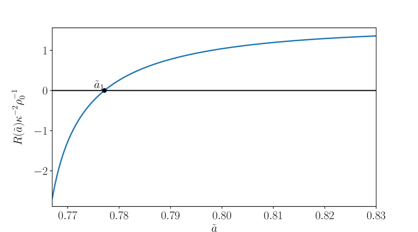
(a) PS I

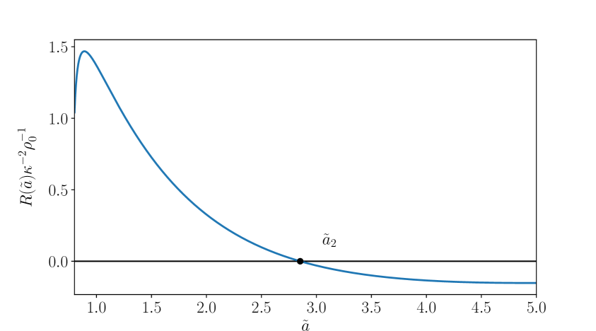
(b) PS II

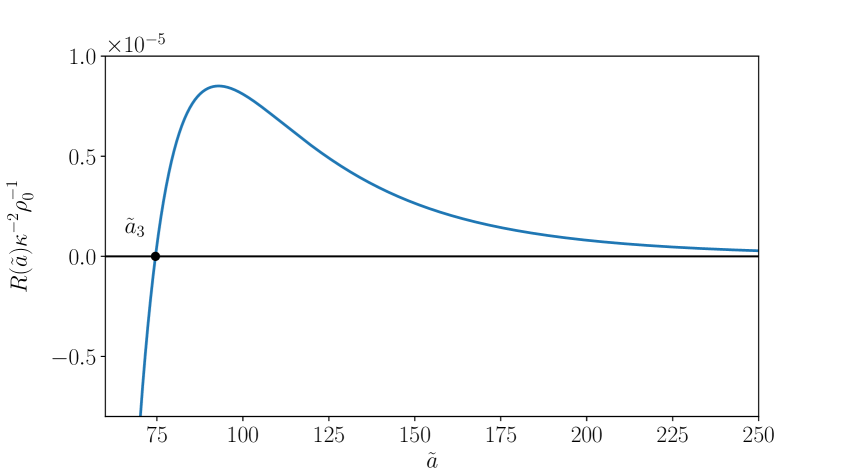
(c) PS III

Figure 1: Jordan frame Ricci scalar as a function of Einstein frame scale factor, $R(\tilde{a})$, with quintessence parameters $(w_{0},w^{\prime})=(-0.87,-0.48)$. The ansatz (3.21) is applicable in the neighborhood of the roots $\tilde{a}_{1,2,3}$. In the limit $\tilde{a}\to 0$, Jordan frame Ricci $R\to 0$.

Each of the solutions for the ansatz $F_{A}$ (3.21), i.e., Parameter set I (PS I), Parameter set II (PS II), Parameter set III (PS III), is applicable in the neighborhood of one of the points $\tilde{a}_{1,2,3}$, where $R(\tilde{a})\to 0$ (see table 1). We compare the exact $F(\tilde{a})$ (from (3.24)) with $F_{A}(\tilde{a})$ in these neighborhoods in Fig. 2.

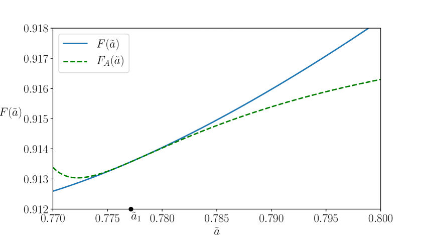
(a) PS I

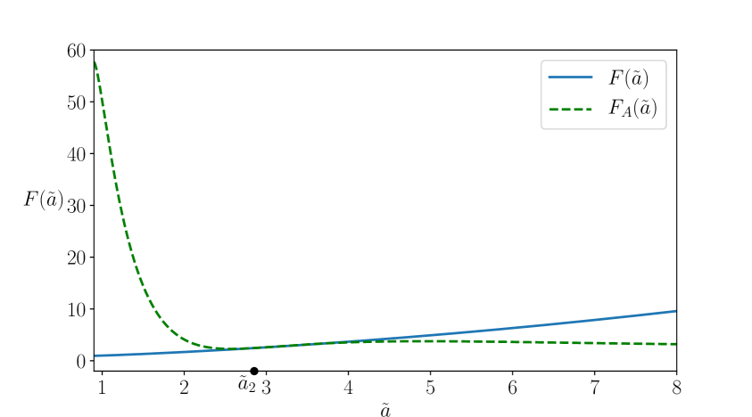
(b) PS II

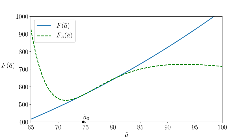
(c) PS III

Figure 2: Comparison of $F(\tilde{a})$ and $F_{A}(\tilde{a})$ for quintessence parameters $(w_{0},w^{\prime})=(-0.87,-0.48)$. The points $\tilde{a}_{1,2,3}$ are the roots of the Jordan Ricci $R(\tilde{a})$. The ansatz $F_{A}(\tilde{a})$, with the solutions PS I, PS II, and PS III, coincides with $F(\tilde{a})$ in the neighborhoods of $\tilde{a}_{1},\tilde{a}_{2},$ and $\tilde{a}_{3}$ respectively.

The best estimation for the ansatz, $F_{A}$, consistent with the current Einstein frame scale factor, $\tilde{a}=1$, is given by the PS I solutions, since $\tilde{a}_{1}$ is the nearest root of $R(\tilde{a})$ to the current scale factor $\tilde{a}=1$. One can estimate the current value of Jordan Ricci using the quintessence parameters (3.22),

$$R_{0}=R(\tilde{a}=1)=1.3684\kappa^{2}\rho_{0}.$$ (3.29)

In order to see whether the ansatz (3.21), with PS I solutions, is consistent at the current universe ($\tilde{a}\to 1$), we derive the relative contributions of the terms in $F_{A}(R)$. Using PS I from table 1 and (3.29) we derive the three terms in the ansatz $F_{A}(R_{0})$,

$$\text{Term}_{0} =\epsilon_{0}=0.91357,$$ (3.30a)

$$\text{Term}_{1} =\epsilon_{1}R_{0}=0.00207,$$ (3.30b)

$$\text{Term}_{2} =\epsilon_{2}R_{0}^{2}=0.00205.$$ (3.30c)

As we can see, the zeroth order term ($\epsilon_{0}$) contributes in the order of $\sim 10^{2}$ times than the first order term ($\epsilon_{1}R_{0}$), however, the contributions of the first order term and the second order term $\epsilon_{2}R_{0}^{2}$ are in the same order of magnitude. The specific deviation of the ansatz $F_{A}(\tilde{a})$ from the exact $F(\tilde{a})$ at current scale factor is

$$\Delta(\tilde{a}=1,\ \text{PS}_{\text{I}})=\frac{|F_{A}(\tilde{a}=1;\ \text{PS}_{\text{I}})-F(\tilde{a}=1)|}{|F(\tilde{a}=1)|}=0.08236.$$ (3.31)

In the following part we discuss the stability of these perturbative solutions.

Stability of perturbative solutions.

For the perturbative solutions $F_{A}(R)$, using quintessence parameters (3.22) we numerically find that $F_{A}>0$ in the limit $\tilde{a}\to\tilde{a}_{1,2,3}$, that is, for solutions corresponding to PS I, PS II, PS III (see table 1). Using the PS I solutions for current Einstein frame universe ($\tilde{a}\to 1$), we find that $F_{A}>0$ in the current epoch as well. We also find that $F_{A}^{\prime}=\epsilon_{1}+2\epsilon_{2}R$ is positive while $\tilde{a}\to\tilde{a}_{1,3}$, however, $F_{A}^{\prime}<0$ as $\tilde{a}\to\tilde{a}_{2}$. For the present day universe ($\tilde{a}=1$), we find $F_{A}^{\prime}>0$ with the PS I solutions.

3.3.2 Asymptotic solution for $F(R)$ in the late time

We first consider the late time behaviour of the scale factor in the Einstein frame. According to our choice of parameterization (2.12), $w(\tilde{a})$ increases monotonically with the scale factor $\tilde{a}$. When $\tilde{a}>\exp\left((1+3w_{0})/(3w^{\prime})\right)$, $w(\tilde{a})>-1/3$, and the quintessence field can no longer drive the acceleration in the Einstein frame. From the Friedmann equation in the Einstein frame,

$$\tilde{H}=\frac{1}{\tilde{a}}\diff{\tilde{a}}{\tilde{t}}=\frac{\kappa^{2}}{3}\rho(\tilde{a}),$$ (3.32)

together with the solution of the continuity equation, $\rho(\tilde{a})=\rho_{0}\tilde{a}^{-3(1+w_{0})+\frac{3}{2}w^{\prime}\ln\tilde{a}}$, it is evident that the $\operatorname{d\!}\tilde{a}/\operatorname{d\!}\tilde{t}$ always remains positive. Therefore, even though the acceleration in the Einstein frame stops at some finite time, the scale factor $\tilde{a}$ keeps increasing indefinitely. Solving the Friedmann equation we find the relation between the coordinate time $\tilde{t}$ and the scale factor to be

$$\tilde{t} =\sqrt{\frac{3}{\kappa^{2}\rho_{0}}}\frac{\sqrt{\pi}}{2\sqrt{A_{2}}}\text{e}^{-\frac{B^{2}_{2}}{4A_{2}}}\text{erfi}\left(\sqrt{A_{2}}\ln\tilde{a}-\frac{B_{2}}{2\sqrt{A_{2}}}\right)+\text{constant},$$ (3.33)

where $A_{2}=-3w^{\prime}/4>0$, $B_{2}=-3(1+w_{0})/2$ (recall that $w^{\prime}<0$ is taken through out in order for the field $\varphi$ to be real valued in the $\tilde{a}\to\infty$ limit). It is evident from (3.33) that $\tilde{a}$ monotonically increases with $\tilde{t}$, hence the late time limit in Einstein frame, defined as $\tilde{t}\to\infty$, can also be expressed as $\tilde{a}\to\infty$.

From (3.24) one can see that $F(\tilde{a})\to\infty$ in the late time limit of the Einstein frame ($\tilde{a}\to\infty$). Now let us consider the late time behaviour of Jordan frame Ricci $R(\tilde{a})$. Starting with (3.15),

$$\frac{R(\bar{\varphi{}})}{C}=\exp\left(\bar{\varphi{}}+C_{2}{\mathcal{P}}^{\frac{4}{3}}\right)\left[4-2{\mathcal{P}}^{\frac{2}{3}}+\frac{2}{3}B{\mathcal{P}}^{-\frac{1}{3}}-\frac{8}{3}BC_{2}{\mathcal{P}}^{\frac{1}{3}}+\frac{4}{3}BC_{2}\mathcal{P}\right],$$ (3.34)

we see, $\bar{\varphi{}}=\ln F\to\infty$ in the late time limit, thus the exponential factor in the last equation is dominant in this limit. Moreover, the second term in the argument of the exponential is dominant, which is,

$$C_{2}\mathcal{P}^{\frac{4}{3}}=C_{2}(A-B\bar{\varphi{}})^{\frac{4}{3}}\approx C_{2}(-B\bar{\varphi{}})^{\frac{4}{3}}\to-\infty\ \text{as}\ \bar{\varphi{}}\to\infty.$$ (3.35)

Note that since $w^{\prime}<0$, from (3.16), $B,C_{2}<0$. Using this and taking the late time limit of (3.34), one can conclude that Jordan frame Ricci $R\to 0^{+}$ in the limit $\tilde{a}\to\infty$ (see Fig. 1(c)). Hence, even if in the limit $\tilde{a}\to\infty$ we see $R\to 0^{+}$, we also find $F\to\infty$, which makes the ansatz $F_{A}$ (3.21) insufficient in the late time limit of Einstein frame.

It is possible to derive an asymptotic functional form of $F(R)$ consistent with the late time limit of Einstein frame. Noting that $F,\bar{\varphi{}}\to\infty$ in this limit, we consider only the most dominant terms in each of the factors of $R(\bar{\varphi{}})$ in (3.34) to obtain

$$\lim_{\bar{\varphi{}}\to\infty}\frac{R(\bar{\varphi{}})}{C} \approx N\bar{\varphi{}}\exp\left(-M\bar{\varphi{}}^{\frac{4}{3}}\right),$$ (3.36)

where,

$$B,C_{2} <0,$$ (3.37a)

$$N =-\frac{4}{3}B^{2}C_{2}>0,$$ (3.37b)

$$M =-C_{2}(-B)^{\frac{4}{3}}>0.$$ (3.37c)

Taking $\ln$ of (3.36) we get

$$\ln\left(\frac{R}{C}\right) =\ln(N\bar{\varphi{}})-M\bar{\varphi{}}^{\frac{4}{3}},$$ (3.38)

neglecting the $\ln$ term in RHS,

$$\bar{\varphi{}}_{LT} ={\left[-\frac{1}{M}\ln\left(\frac{R}{C}\right)\right]}^{\frac{3}{4}},$$ (3.39)

$$\text{and }F_{LT}(R) =\exp\left({\left[-\frac{1}{M}\ln\left(\frac{R}{C}\right)\right]}^{\frac{3}{4}}\right).$$ (3.40)

The subscript $LT$ represents the late time of Einstein frame. Hence, as long as $R/C<1$ ($C>0$, as defined in (3.16)), $F_{LT}$ remains real, which is acceptable since this is valid in large $F$ and small $R$ limit. We can plug in $\bar{\varphi{}}$ from (3.39) in (3.14) to get an asymptotic expression for $f(R)$.

$$f(\bar{\varphi{}}) =C\exp\left(2\bar{\varphi{}}+C_{2}\mathcal{P}^{\frac{4}{3}}\right)\left[2-\mathcal{P}^{\frac{2}{3}}+\frac{2}{3}B\mathcal{P}^{-\frac{1}{3}}-\frac{8}{3}BC_{2}\mathcal{P}^{\frac{1}{3}}+\frac{4}{3}BC_{2}\mathcal{P}\right]$$ (3.41a)

$$\approx C\exp\left(C_{2}(-B)^{\frac{4}{3}}\bar{\varphi{}}^{\frac{4}{3}}\right)\left[-\frac{4}{3}B^{2}C_{2}\bar{\varphi{}}\right]$$ (3.41b)

$$f_{LT}(R) =NR\left[-\frac{1}{M}\ln\left(\frac{R}{C}\right)\right]^{\frac{3}{4}}$$ (3.41c)

where in the second line, we have considered only the highest order terms in $\bar{\varphi{}}$ in the argument of the exponential and in the square bracket.

It is evident from (3.40) that for the asymptotic solution $F_{LT}>0$, as long as $0<R/C<1$, this satisfies the ‘positive gravitational coupling’ condition $F>0$. However, $F_{LT}^{\prime}<0$, where

$$F_{LT}^{\prime}=-\frac{3}{4MR}\frac{1}{\left[-\frac{1}{M}\ln\left(\frac{R}{C}\right)\right]^{\frac{1}{4}}}\exp\left(\left[-\frac{1}{M}\ln\left(\frac{R}{C}\right)\right]^{\frac{3}{4}}\right).$$ (3.42)

The late time solution $F_{LT}$ seemingly violates the ‘matter instability condition’ as discussed previously. However, the ‘Dolgov-Kawasaki/matter instability’ condition is not inherently suitable in the late time limit of the current $f(R)$ model. The derivation of the stability condition assumes that the $f(R)$ theory is a small deviation of Einstein gravity (3.17) (see [84, 43] for the derivation), this implies $F(R)=f^{\prime}(R)=1+\varepsilon\psi^{\prime}(R)$. However, for the current model in the late time limit, we see that $F_{LT}(\tilde{a}\to\infty)\to\infty$, it cannot be considered as a perturbation on Einstein gravity.

4 Relation between Jordan and Einstein frame scale factors

In this section we explore the late time relation between the Jordan and Einstein frame scale factors. For the current model, one can obtain the Einstein frame Ricci scalar as

$$\tilde{R}(\tilde{x})=\kappa^{2}\rho_{0}(1-3w_{0}+3w^{\prime}\tilde{x})\exp{\left[-3(1+w_{0})\tilde{x}+\frac{3}{2}w^{\prime}\tilde{x}^{2}\right]},$$ (4.1)

where $\tilde{x}=\ln\tilde{a}$. We can see that the Einstein frame universe becomes Ricci flat in the late time limit, i.e., $\tilde{R}\to 0$ as $\tilde{x}=\ln\tilde{a}\to\infty$ (recall that we consider $w^{\prime}<0$ as discussed before). We have already seen that the Jordan frame Ricci scalar $R$ vanishes in this limit too. However, as the Einstein frame scale factor $\tilde{a}\to\infty$ in the late time limit (see (3.33)), the Jordan frame scale factor $a\to 0$, resulting in a collapsing Jordan frame universe. To see this, consider the relation between the line elements in Einstein ($\operatorname{d\!}\tilde{s}^{2}$) and Jordan ($\operatorname{d\!}s^{2}$) frames [42],

$$\operatorname{d\!}\tilde{s}^{2} =-\operatorname{d\!}\tilde{t}^{2}+\tilde{a}^{2}\operatorname{d\!}\mathbf{\tilde{x}}^{2}$$ (4.2a)

$$=\Omega^{2}\operatorname{d\!}s^{2}$$ (4.2b)

$$=F(-\operatorname{d\!}t^{2}+a^{2}\operatorname{d\!}\mathbf{x}^{2}),$$ (4.2c)

which implies

$$\operatorname{d\!}\tilde{t} =\sqrt{F}\operatorname{d\!}t$$ (4.3)

$$a =\frac{\tilde{a}}{\sqrt{F}}.$$ (4.4)

Using this the Jordan frame scale factor can be written in terms of the Einstein frame scale factor as

$$a(\tilde{a})=\exp(C_{5})\tilde{a}\exp\left(\frac{\sqrt{2}}{3w^{\prime}}(1+w_{0}-w^{\prime}\ln\tilde{a})^{\frac{3}{2}}\right),$$ (4.5)

where $C_{5}=-\frac{\sqrt{2}}{3w^{\prime}}(1+w_{0})^{\frac{3}{2}}$, equation (3.24) is used to derive the last equation. $a(\tilde{a})$ reaches the maximum value at $\tilde{a}=\exp((w_{0}-1)/w^{\prime})$, after which it decreases monotonically. For the quintessence parameters in (3.22), $a(\tilde{a})$ becomes maximum as $\tilde{a}\to 49.197$. In the late time limit of the Einstein frame ($\tilde{a}\to\infty$), the Jordan frame scale factor $a\to 0$ for $w^{\prime}<0$ (see Fig. 3).

This result leads to two interesting observations. First, the Jordan frame scale factor has a maximum value at the critical point $w(\tilde{a})=1$, this means the Jordan frame universe has a bound on its spatial size, which is determined by the quintessence parameters ($w_{0},w^{\prime}$). This is in contrast with the Einstein frame universe, as we have seen in (3.33), the Einstein frame scale factor grows indefinitely with the coordinate time. Second, the collapsing universe in the Jordan frame provides an equivalent description of the expanding universe in the Einstein frame. This map between collapsing and expanding frames can be a useful tool. For example, introducing metric perturbations in the backgrounds of the FRW spacetime, one may establish a relation between the perturbation in the expanding frame with the perturbation in the collapsing frame. Perturbation in a collapsing gravitational system can be analyzed within the $f(R)$ setting [85]. Further studies can reveal how the quantum effects in the collapsing Jordan frame correspond to the perturbations in the ever-expanding Einstein frame at late times (see, for example, [86, 87, 88, 89, 90] and references therein). These issues will be pursued elsewhere.

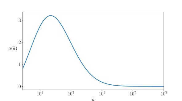
Figure 3: Late time collapse of the Jordan frame universe. For a quintessence model with logarithmic equation of state parameter, $w(\tilde{a})=w_{0}-w^{\prime}\ln\tilde{a},\ w^{\prime}<0$. The Jordan frame scale factor plotted as a function of the Einstein frame scale factor, $a(\tilde{a})$, with quintessence parameters $(w_{0},w^{\prime})=(-0.87,-0.48)$. $a(\tilde{a})$ has a maximum at $\tilde{a}=\exp((w_{0}-1)/w^{\prime})=49.197$. In the late time limit $a\to 0$ as $\tilde{a}\to\infty$.

5 Expansion-collapse duality in the presence of non-relativistic matter

While discussing the expansion-collapse duality of the two conformally connected frames, we have so far considered the quintessence field to be the only component in the Einstein frame universe. In this section we consider a more realistic scenario where the Einstein frame universe consists of the quintessence field as well as matter. Although dark energy is the dominant component of the current epoch, even the subdominant presence of dust (non-relativistic pressureless fluid) staggers the Jordan frame collapse.

Since we are considering the Einstein frame to be the physical frame; observations are made in this frame. Therefore, leaning to the standard considerations, in the Einstein frame matter is minimally coupled to gravity, there is no explicit coupling between matter and the quintessence field $\varphi$. Since the Einstein and Jordan frames are conformally related, the couplings transform non-trivially between the frames– that matter will be non-minimally coupled to gravity in the Jordan frame. Therefore, for a more realistic description of the Einstein frame, the total Jordan frame action will have a form

$$\mathcal{S}_{J} =\frac{1}{2\kappa^{2}}\int d^{4}x\sqrt{-g}f(R)+\int d^{4}x\sqrt{-g}F^{2}(R)\mathcal{L}_{\text{M}}(\psi_{\text{M}};F(R)g_{\mu\nu}).$$ (5.1)

Since $F(R)=\partial f/\partial R$, the matter-gravity coupling is through some function of Ricci scalar and belongs to a broad class of curvature couplings [91]. This form of the action in the Jordan frame is chosen such that, after conformal transformation $\tilde{g}_{\mu\nu}=Fg_{\mu\nu}$, matter decouples from the curvature $\tilde{R}$ in the Einstein frame,

$$\mathcal{S}_{E}=\int d^{4}x\sqrt{-\tilde{g}}\frac{1}{2\kappa^{2}}\tilde{R}-\int d^{4}x\sqrt{-\tilde{g}}\left[\frac{1}{2}\tilde{g}^{\mu\nu}\partial_{\mu}\varphi\partial_{\nu}\varphi+V(\varphi)\right]+\int d^{4}x\sqrt{-\tilde{g}}\mathcal{L}_{\text{M}}(\psi_{\text{M}};\tilde{g}_{\mu\nu}).$$ (5.2)

Due to introduction of matter, solutions for the Jordan frame action obtained previously for the case of pure gravity in Jordan frame will not be consistent with action (5.1). Thus the equation of motion, condition for acceleration and the relation between the two frames’ scale factor will be modified, however we will see that the explicit form of the solution of this action does not affect the existence of the expansion-collapse duality. Thus, the existence of such duality between the frames can be considered to be a robust feature.

From the Einstein frame action (5.2), one can obtain the usual Friedmann equation

$$\tilde{H}^{2}=\frac{\kappa^{2}}{3}\left(\rho_{m}+\rho_{\varphi}\right),$$ (5.3)

where $\tilde{H}$ is the Hubble parameter in the Einstein frame, $\rho_{m}$ and $\rho_{\varphi}$ are the energy densities corresponding to dust and the quintessence field respectively. Together with observationally consistent values of ($\Omega_{m0},\Omega_{\varphi 0},w_{\varphi}$), Eq. (5.3) correctly reproduces the standard expansion history of the universe without spatial curvature in the Einstein frame. The case with spatial curvature is discussed later.

Using (5.3) in (2.6) for the Einstein frame we obtain

$$\diff{\Phi}{\tilde{a}}=\frac{\sqrt{3}}{\kappa}\frac{1}{\tilde{a}}\sqrt{\frac{1+w_{\varphi}(\tilde{a})}{1+\rho_{m}/\rho_{\varphi}}},$$ (5.4)

where $w_{\varphi}$ is the equation of state parameter of the quintessence field. This, together with (4.4), leads to a relation between the Jordan and the Einstein frame scale factors ($a,\ \tilde{a}$),

$$a(\tilde{a})=\tilde{a}\exp\left(-\frac{1}{\sqrt{2}}\int_{1}^{\tilde{a}}\frac{d\tilde{a}^{\prime}}{\tilde{a}^{\prime}}\sqrt{\frac{1+w_{\varphi}}{1+\rho_{m}/\rho_{\varphi}}}\right).$$ (5.5)

For the logarithmic $w_{\varphi}$ (2.12), the above equation becomes

$$a(\tilde{a})=\tilde{a}\exp\left(-\frac{1}{\sqrt{2}}\int_{1}^{\tilde{a}}\frac{d\tilde{a}^{\prime}}{\tilde{a}^{\prime}}\sqrt{\frac{1+w_{0}-w^{\prime}\ln\tilde{a}^{\prime}}{1+\Omega_{r}\exp\left(3w_{0}\ln\tilde{a}^{\prime}-\frac{3}{2}w^{\prime}(\ln\tilde{a}^{\prime})^{2}\right)}}\right),$$ (5.6)

where we have used $\rho_{m}=\rho_{m0}\tilde{a}^{-3}$, $\rho_{\varphi}=\rho_{\varphi 0}\tilde{a}^{-3(1+w_{0})+\frac{3}{2}w^{\prime}\ln\tilde{a}}$, $\Omega_{r}=\Omega_{m0}/\Omega_{\varphi 0}=\rho_{mo}/\rho_{\varphi 0}$, and $\Omega_{m0,\varphi 0}$ are the density parameters corresponding to dust and the quintessence field at $\tilde{a}=1$. For $\Omega_{r}=0$, that is, if the energy contribution of dust is completely neglected, the equation (5.6) can be solved analytically, resulting in (5.3) as is expected. However, for nonzero $\Omega_{r}$, equation (5.6) can be solved only numerically. Fig. 4 shows the evolution of the Jordan frame scale factor with respect to the Einstein frame scale factor for different values of $\Omega_{r}$. We see that even if the energy contribution due to dust with respect to that of the quintessence field is taken to be as small as $\Omega_{r}=10^{-8}$ at the current epoch, the Jordan frame collapse sustains only for a finite duration of time. Eventually in the late times of the Einstein frame, Jordan frame scale factor turns around and starts to increase monotonically. For the value of the dust-dark energy ratio consistent with observation, $\Omega_{r}\sim 0.3/0.7$, we see that the Jordan frame universe never collapses, the Jordan frame scale factor evolves monotonically with respect to the Einstein frame scale factor.

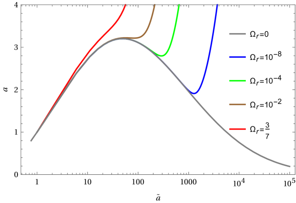
Figure 4: Evolution of Jordan frame scale factor $a$ with respect to Einstein frame scale factor $\tilde{a}$ for different values of $\Omega_{r}$, where $\Omega_{r}=\Omega_{m0}/\Omega_{\varphi 0}$ is the ratio of the density parameters of dust and the quintessence field at the current epoch $\tilde{a}=1$ and $(w_{0},w^{\prime})=(-0.87,-0.48)$. Any non zero value of $\Omega_{m0}$ prevents the Jordan frame universe to collapse indefinitely. For $\Omega_{r}$ consistent with observations, $\Omega_{r}=\Omega_{m0}/\Omega_{\varphi 0}\sim 0.3/0.7$, the Jordan frame expands monotonically with respect to the Einstein frame.

In fact, it is generally possible to write the condition for the Jordan frame collapse in a relatively simple inequality. Starting with (4.4) we can obtain the derivative of Jordan frame scale factor with respect to that of the Einstein frame,

$$\diff{a}{\tilde{a}}=\diff{}{\tilde{a}}\left(\frac{\tilde{a}}{\sqrt{F}}\right)=F^{-1/2}\left(1-\kappa\sqrt{1+w_{\varphi}(\tilde{a})}\sqrt{\frac{\rho_{\varphi}}{6\tilde{H}^{2}}}\right),$$ (5.7)

where we have used the Einstein-Jordan frame correspondence, $2\kappa\varphi=\sqrt{6}\ln F$, along with the result

$$\diff{\varphi}{\tilde{a}}=\frac{1}{\tilde{a}}\sqrt{1+w_{\varphi}(\tilde{a})}\sqrt{\frac{\rho_{\varphi}}{\tilde{H}^{2}}}.$$ (5.8)

It is evident from (5.7) that the Jordan frame universe collapses, that is, $\operatorname{d\!}a/\operatorname{d\!}\tilde{a}<0$ if and only if the following inequality is satisfied,

$$w_{\varphi}(\tilde{a}) >\mathcal{C}(\tilde{a})$$ (5.9a)

$$\mathcal{C}(\tilde{a}) =\frac{6\tilde{H}^{2}}{\kappa^{2}\rho_{\varphi}(\tilde{a})}-1.$$ (5.9b)

The above condition leads to a range (or possibly multiple ranges) of $\tilde{a}$ during which the Jordan frame collapses. This also shows that in order for the Jordan frame to have a ‘turn around’, that is where $\operatorname{d\!}a/\operatorname{d\!}\tilde{a}=0$, the equation $w_{\varphi}(\tilde{a})=\mathcal{C}(\tilde{a})$ must have a solution. This is applicable for arbitrary quintessence models; it also takes into account the presence of any other component in the universe, like dust, radiation or spatial curvature. However, it is to be noted that the condition is only imposed on $w_{\varphi}$, not on the effective equation of state parameter of the era and the existence of all the other components is incorporated in the Hubble parameter $\tilde{H}$, through the Friedmann equation. We also point out that this inequality has a significantly simple form. Starting with any given $w_{\varphi}(\tilde{a})$, one can check whether the condition is satisfied just by knowing $\rho_{\varphi}(\tilde{a})$. The functional form of $f(R)$, the solution of the quintessence field $\varphi(\tilde{a})$ or even the form of the potential $V(\varphi)$ are not required for that matter. Further, we see from Eq. (5.7) the condition $da/d\tilde{a}<0$ is insensitive to exact from of $F(R)$ which also plays the role of non-minimal coupling in the Jordan frame, but is solely decided by the ratio $6\tilde{H}^{2}/\kappa^{2}\rho_{\varphi}(\tilde{a})$, i.e. on the phenomenological form of the quintessence field arrived at in the Einstein frame. Thus, the onset of collapse in the Jordan frame remains persistent even in the presence of the proposed non-minimal coupling.

For the quintessence model under discussion, the inequality (5.9a) takes the form

$$w_{\varphi}(\tilde{a}) >\mathcal{C}(\tilde{a})\text{, where}$$ (5.10a)

$$w_{\varphi}(\tilde{a}) =w_{0}-w^{\prime}\ln\tilde{a},$$ (5.10b)

$$\mathcal{C}(\tilde{a}) =1+2\frac{\Omega_{m0}}{\Omega_{\varphi 0}}\exp\left(3w_{0}\ln\tilde{a}-\frac{3}{2}w^{\prime}(\ln\tilde{a})^{2}\right).$$ (5.10c)

in the presence of matter. For the values of the parameters $(w_{0},w^{\prime},\Omega_{m0})$ consistent with observations, one can argue that the above inequality is never satisfied (see Appendix B for the argument), thus the quintessence model with logarithmic equation of state parameter does not lead to a collapsing Jordan frame in the presence of dust.

We conclude this section by discussing the effect of a positive spatial curvature on the expansion-collapse duality. As it is argued in [68], the latest Planck data [92] appears to be consistent with a universe possessing a small positive spatial curvature. We find that the introduction of a positive spatial curvature in the analysis above recovers the expansion collapse duality in the presence of dust. Taking into account both spatial curvature and dust, the Friedmann equation in the Einstein frame becomes

$$\tilde{H}^{2}=\frac{\kappa^{2}}{3}\left(\rho_{\varphi}+\rho_{m}\right)-\frac{K}{\tilde{a}^{2}},$$ (5.11)

where $K$ is the spatial curvature parameter appearing in the FRW metric. In this case the condition of expansion-collapse duality (5.9a) becomes

$$w_{\varphi}(\tilde{a}) >\mathcal{C}(\tilde{a})\text{, where}$$ (5.12a)

$$w_{\varphi}(\tilde{a}) =w_{0}-w^{\prime}\ln\tilde{a},$$ (5.12b)

$$\mathcal{C}(\tilde{a}) =1+2\frac{\Omega_{m0}}{\Omega_{\varphi 0}}\exp\left(3w_{0}\ln\tilde{a}-\frac{3}{2}w^{\prime}(\ln\tilde{a})^{2}\right)$$

$$+2\frac{\Omega_{K0}}{\Omega_{\varphi 0}}\exp\left((1+3w_{0})\ln\tilde{a}-\frac{3}{2}w^{\prime}(\ln\tilde{a})^{2}\right),$$ (5.12c)

where $\Omega_{K}=-K/(\tilde{a}\tilde{H})^{2}$, $\Omega_{K0}=-K/\tilde{H}_{0}^{2}$ is the current value of the density parameter associated with the spatial curvature. As we can see from the condition, introduction of a positive spatial curvature, that is, a negative $\Omega_{K}$, brings down the threshold that $w_{\varphi}$ is required to cross in order for the Jordan frame collapse to begin. For example, with the value $\Omega_{K0}=-.0438$ [68], Fig. 5 shows region of $\tilde{a}$ where the condition for Jordan frame collapse is satisfied in the presence of matter.

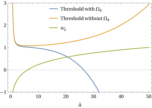
Figure 5: Possibility of Jordan frame collapse in the presence of positive spatial curvature and dust, with $(w_{0},w^{\prime})=(-0.87,-0.48),\ \Omega_{m0}=0.315,\ \Omega_{\varphi 0}=.728,\ \Omega_{K0}=-.043$. ‘Threshold’ refers to the function $\mathcal{C}$ in (5.12a). The Jordan frame collapse while $w_{\varphi}(\tilde{a})>\mathcal{C}(\tilde{a})$ is satisfied. The plot shows that in contrast with the case when $\Omega_{k}=0$, the negative contribution from $\Omega_{K}$ brings down the threshold $\mathcal{C}$ eventually. This allows for $w_{\varphi}$ to cross the threshold at $\tilde{a}\sim 20.52$, after which the Jordan frame starts to collapse.

To summarize, we show that the quintessence model with logarithmic equation of state parameter leads to an expansion-collapse duality between Einstein and Jordan frames, that is, while the Einstein frame expands indefinitely, the Jordan frame collapses in the late time. We generalize the requirement of this expansion-collapse duality for arbitrary quintessence models, taking into account the presence of other components in the Einstein frame as well. This requirement essentially imposes a threshold on the equation of state parameter of the quintessence field, the threshold itself is determined by the form of energy densities associated with all the components in the Einstein frame universe. Using this we find that the Jordan frame collapse gradually becomes short lived if dust is included in the Einstein frame universe. However, the Jordan frame collapse, at least for a finite duration, can be recovered by introducing a small positive spatial curvature.

6 Conclusion and discussion

Quintessence fields are viable alternatives to the $\Lambda$CDM models, which can provide an explanation for the recent accelerated expansion of the universe. It is known that an $f(R)$ theory of gravity in the Jordan frame acts as a dual to a quintessence field in Einstein gravity, in a conformally connected spacetime, known as the Einstein frame. In this work, we reconstruct $f(R)$ functions in Jordan frame which reproduce quintessence models with time-independent and time-dependent equation of state parameter ($w$) in the Einstein frame.

As an example of time-dependent equation of state parameter, we choose the logarithmic parameterization and reconstruct $f(R)$ function corresponding to the quintessence model. This solution is obtained in two parts. A perturbative solution of $F(R)$ is obtained which is valid in the small curvature limit of the Jordan frame. We show that this perturbative solution may be applicable in the near future of the Einstein frame universe. However, we find that this ansatz becomes ill-defined in the late time limit of Einstein frame. We obtain an asymptotic solution for $f(R)$, which is valid in large field and small curvature limit of the Jordan frame. This asymptotic solution is applicable in the late time limit of the Einstein frame. We also show that the Jordan frame scale factor has a finite maximum value determined by the quintessence model parameters, after which it keeps on decreasing. In the late time limit of the Einstein frame, the Jordan frame universe collapses while the expansion in the Einstein frame universe continues.

We generalize this result and obtain the condition for expansion-collapse duality in terms of a simple inequality. This condition can predict the possibility of Jordan frame collapse for quintessence models with arbitrary equation of state parameters, even in the presence of other components in the universe such as dust, radiation or spatial curvature. Given an equation of state parameter, such prediction can be made only from the knowledge of energy density of the quintessence model. Using this condition we show that the example quintessence model does not necessarily lead to the Jordan frame collapse in the presence of dust, however the expansion-collapse duality may be recovered by introducing a positive spatial curvature component in the universe.

The general condition for expansion-collapse duality can be readily applied to other physically viable quintessence models. This opens a possibility of further studies of the collapse of the Jordan frame. The mapping between expanding and collapsing geometries may have implications on growth of perturbations which is a subject of further exploration.

Appendix A Analytical results for the perturbative solution $F_{A}$

Here we present the solutions of the ansatz (3.21), i.e., we write the constants $\epsilon_{0},\epsilon_{1},\epsilon_{2}$ in terms of the quintessence parameters $w_{0},w^{\prime}$. We use the ansatz (3.21) in the RHS of (3.15) and ignore terms of the order $R^{2}$ and higher to obtain

$$\begin{split}R=\ &C\alpha_{0}\beta_{0}\epsilon_{0}+C\left[\alpha_{1}\beta_{0}\epsilon_{0}+\alpha_{0}\beta_{0}\epsilon_{1}+\alpha_{0}\beta_{1}\epsilon_{0}\right]R\\ &+\ C\left[\alpha_{2}\beta_{0}\epsilon_{0}+\alpha_{1}\beta_{0}\epsilon_{1}+\alpha_{0}\beta_{0}\epsilon_{2}+\alpha_{1}\beta_{1}\epsilon_{0}+\alpha_{0}\beta_{1}\epsilon_{1}+\alpha_{0}\beta_{2}\epsilon_{0}\right]R^{2},\end{split}$$ (A.1)

where we have defined the following terms

$$k_{0} =A-B\ln\epsilon_{0}$$ (A.2a)

$$k_{1} =-B\frac{\epsilon_{1}}{\epsilon_{0}}$$ (A.2b)

$$k_{2} =-B\left(\frac{\epsilon_{2}}{\epsilon_{0}}-\frac{\epsilon_{1}^{2}}{2\epsilon_{0}^{2}}\right),$$ (A.2c)

$$\alpha_{0} =e^{C_{2}k_{0}^{\frac{4}{3}}}$$ (A.3a)

$$\alpha_{1} =\frac{4}{3}C_{2}k_{0}^{\frac{1}{3}}k_{1}e^{C_{2}k_{0}^{\frac{4}{3}}}$$ (A.3b)

$$\alpha_{2} =\left[\frac{4}{3}C_{2}k_{0}^{\frac{1}{3}}k_{2}+\frac{2}{9}C_{2}k_{1}^{2}k_{0}^{-\frac{2}{3}}+\frac{8}{9}C_{2}^{2}k_{0}^{\frac{2}{3}}k_{1}^{2}\right]e^{C_{2}k_{0}^{\frac{4}{3}}},$$ (A.3c)

and

$$\beta{}_{0}= +4-\frac{8}{3}BC_{2}k_{0}^{\frac{1}{3}}+\frac{2}{3}Bk_{0}^{-\frac{1}{3}}-2k_{0}^{\frac{2}{3}}+\frac{4}{3}BC_{2}k_{0}$$ (A.4a)

$$\beta{}_{1}= -\frac{8}{9}BC_{2}k_{1}k_{0}^{-\frac{2}{3}}-\frac{2}{9}Bk_{1}k_{0}^{-\frac{4}{3}}-\frac{4}{3}k_{1}k_{0}^{-\frac{1}{3}}+\frac{4}{3}BC_{2}k_{1}$$ (A.4b)

$$\beta_{2}= -\frac{8}{9}BC_{2}k_{2}k_{0}^{-\frac{2}{3}}+\frac{8}{27}BC_{2}k_{1}^{2}k_{0}^{-\frac{5}{3}}-\frac{2}{9}Bk_{2}k_{0}^{-\frac{4}{3}}+\frac{4}{27}Bk_{1}^{2}k_{0}^{-\frac{7}{3}}$$

$$-\frac{4}{3}k_{2}k_{0}^{-\frac{1}{3}}+\frac{2}{9}k_{1}^{2}k_{0}^{-\frac{4}{3}}+\frac{4}{3}BC_{2}k_{2}.$$ (A.4c)

The terms $A,B,C_{1},C_{2},C$ were defined in (3.16). Now we can compare the coefficients of different powers of $R$ in (A.1) to determine the $\epsilon_{0,1,2}(w0,w^{\prime})$. Comparing the coefficients of $R^{0}$ we find

$$f_{0}(\epsilon_{0})=\alpha_{0}\beta_{0}\epsilon_{0}=0.$$ (A.5)

Form (A.3) we seen $\alpha_{0}\neq 0$, (A.5) becomes

$$\beta_{0} =0$$ (A.6a)

$$4-\frac{8}{3}BC_{2}k_{0}^{\frac{1}{3}}+\frac{2}{3}Bk_{0}^{-\frac{1}{3}}-2k_{0}^{\frac{2}{3}}+\frac{4}{3}BC_{2}k_{0} =0$$ (A.6b)

$$4k_{0}^{\frac{1}{3}}-\frac{8}{3}BC_{2}k_{0}^{\frac{2}{3}}+\frac{2}{3}B-2k_{0}+\frac{4}{3}BC_{2}k_{0}^{\frac{4}{3}} =0$$ (A.6c)

$$\frac{3}{BC_{2}}k_{0}^{\frac{1}{3}}-2k_{0}^{\frac{2}{3}}+\frac{1}{2C_{2}}-\frac{3}{2BC_{2}}k_{0}+k_{0}^{\frac{4}{3}} =0$$ (A.6d)

{putting $$k_{0}^{\frac{1}{3}}=x (BC_{2})^{-1}=m (2C_{2})^{-1}=n$$, , }

$$x^{4}-\frac{3}{2}mx^{3}-2x^{2}+3mx+n =0.$$ (A.6e)

Solutions of this quartic equation lead to $\epsilon_{0}$. That is, for a given set of $w_{0},w^{\prime}$, it is possible to get multiple solutions for $\epsilon_{0}$. Once $\epsilon_{0}$ is known, comparing the coefficients of $R^{1}$ in (A.1) one can obtain $\epsilon_{1}$ as

$$f_{1}(\epsilon_{0},\epsilon_{1}) =\alpha_{0}\beta_{1}\epsilon_{0}-\frac{1}{C}=0$$ (A.7a)

$$\epsilon_{1} =\frac{1}{B\alpha_{0}C\left(\frac{8}{9}BC_{2}k_{0}^{-\frac{2}{3}}+\frac{2}{9}Bk_{0}^{-\frac{4}{3}}+\frac{4}{3}k_{0}^{-\frac{1}{3}}-\frac{4}{3}BC_{2}\right)}.$$ (A.7b)

Finally, with $\epsilon_{0},\epsilon_{1}$ known, $\epsilon_{2}$ can be obtained by comparing the coefficients of $R^{2}$,

$$f_{2}(\epsilon_{0},\epsilon_{1},\epsilon_{2}) =\alpha_{1}\beta_{1}\epsilon_{0}+\alpha_{0}\beta_{1}\epsilon_{1}+\alpha_{0}\beta_{2}\epsilon_{0}=0$$ (A.8a)

$$\epsilon_{2} =\frac{\epsilon_{1}^{2}}{2\epsilon_{0}}+\frac{\epsilon_{0}}{B}\frac{\frac{8}{27}BC_{2}k_{1}^{2}k_{0}^{-\frac{5}{3}}+\frac{4}{27}Bk_{1}^{2}k_{0}^{-\frac{7}{3}}+\frac{2}{9}k_{1}^{2}k_{0}^{-\frac{4}{3}}+\beta_{1}\left(\frac{\alpha_{1}}{\alpha_{0}}-\frac{\epsilon_{1}}{\epsilon_{0}}\right)}{-\frac{8}{9}BC_{2}k_{0}^{-\frac{2}{3}}-\frac{2}{9}Bk_{0}^{-\frac{4}{3}}+\frac{4}{3}BC_{2}-\frac{4}{3}k_{0}^{-\frac{1}{3}}}.$$ (A.8b)

Appendix B Condition for Jordan frame collapse in the presence of dust

Here we argue that Jordan frame collapse is not possible in a spatially flat universe consisting of dust and a quintessence field with logarithmic $w_{\varphi}$. We start with the general condition for collapse in the presence of dust, with $\Omega_{K0}=0$, from (5.10a)

$$w_{\varphi}(\tilde{a})>\mathcal{C}(\tilde{a})$$ (B.1)

where,

$$w_{\varphi}(\tilde{a}) =w_{0}-w^{\prime}\ln\tilde{a},$$ (B.2a)

$$\mathcal{C}(\tilde{a}) =1+2\frac{\rho_{m}}{\rho_{\varphi}}$$ (B.2b)

$$=1+2\frac{\Omega_{m0}}{\Omega_{\varphi 0}}\exp\left(3w_{0}\ln\tilde{a}-\frac{3}{2}w^{\prime}(\ln\tilde{a})^{2}\right)$$ (B.2c)

$$=1+2\Omega_{r}\exp\left(3w_{0}\ln\tilde{a}-\frac{3}{2}w^{\prime}(\ln\tilde{a})^{2}\right).$$ (B.2d)

Let us now consider the following arguments

1. It is obvious from (B.2b) that $\mathcal{C}(\tilde{a})$ has a lower bound of $1$, $\mathcal{C}>1$. Since $w_{\varphi}(\tilde{a})$ is a monotonically increasing function of $\tilde{a}$, $w_{\varphi}$ can intersect with $\mathcal{C}$ only after $w_{\varphi}$ crosses $1$. This happens at

   $$\tilde{a}_{*}=\exp\left(\frac{w_{0}}{w^{\prime}}-\frac{1}{w^{\prime}}\right).$$ (B.3)

   Thus, it is sufficient to consider only the range $\tilde{a}>\tilde{a}_{*}$ in order to check the possibility of the intersection.

2. The slopes of these functions are given by

   $$w_{\varphi,\tilde{a}}(\tilde{a}) =\frac{-w^{\prime}}{\tilde{a}}$$ (B.4a)

   $$\mathcal{C}_{,\tilde{a}}(\tilde{a}) =6\Omega_{r}(w_{0}-w^{\prime}\ln\tilde{a})\exp\left((3w_{0}-1)\ln\tilde{a}-\frac{3}{2}w^{\prime}(\ln\tilde{a})^{2}\right).$$ (B.4b)

   Where the subscript $,\tilde{a}$ denotes the derivatives of the functions with respect to $\tilde{a}$.

3. At the point $\tilde{a}_{*}$, the slope of $\mathcal{C}$ is higher than the slope of $w_{\varphi}$. To see this consider the ratio of the slopes

   $$\frac{\mathcal{C}_{,\tilde{a}}}{w_{\varphi,\tilde{a}}}=-\frac{6\Omega_{r}}{w^{\prime}}\left(w_{0}-w^{\prime}\ln\tilde{a}\right)\exp\left(3w_{0}\ln\tilde{a}-\frac{3}{2}w^{\prime}(\ln\tilde{a})^{2}\right).$$ (B.5)

   At the point $\tilde{a}_{*}$, this ratio becomes

   $$\left.\frac{\mathcal{C}_{,\tilde{a}}}{w_{\varphi,\tilde{a}}}\right|_{\tilde{a}=\tilde{a}_{*}}=-\frac{6\Omega_{r}}{w^{\prime}}\exp\left(\frac{3}{2w^{\prime}}(w_{0}^{2}-1)\right)$$ (B.6)

   The observationally consistent range of $w_{0}$ (2.13) is $-1.09<w_{0}<-0.66$. However we do not consider the possibility of $-1>w_{0}$ because this does not lead to a real $\varphi$ (2.15). Now for $-1<w_{0}<0$ and $w^{\prime}<0$, the argument of the exponential is non-negative. The minimum possible value of the RHS is obtained when $w^{\prime}$ is most negative and $\Omega_{mo}$ is smallest. Putting $w_{0}=-1,\ w^{\prime}=-1.22,\Omega_{r}=.26/(1-.26)$ we get

   $$\left.\frac{\mathcal{C}_{,\tilde{a}}}{w_{\varphi,\tilde{a}}}\right|_{\tilde{a}=\tilde{a}_{*}}=1.73.$$ (B.7)

   Thus we conclude that at $\tilde{a}_{*}$, $\mathcal{C}$ has a higher slope than $w_{\varphi}$ given our choice of parameters.

4. In the range $\tilde{a}>\tilde{a}_{*}$, the slope of $w_{\varphi}(\tilde{a})$ always decreases. This is obvious since

   $$w_{,\tilde{a}\tilde{a}}=\frac{w^{\prime}}{\tilde{a}^{2}}<0.$$ (B.8)

   On the other hand

   $$\mathcal{C}_{,\tilde{a}\tilde{a}} =6\Omega_{r}\exp\left((3w_{0}-2)\ln\tilde{a}-\frac{3}{2}w^{\prime}(\ln\tilde{a})^{2}\right)\left[3w^{\prime 2}(\ln\tilde{a})^{2}+(w^{\prime}-6w_{0}w^{\prime})\ln\tilde{a}+3w_{0}^{2}-w_{0}-w^{\prime}\right]$$ (B.9)

   $$\mathcal{C}_{,\tilde{a}\tilde{a}} =6\Omega_{r}\exp\left((3w_{0}-2)\ln\tilde{a}-\frac{3}{2}w^{\prime}(\ln\tilde{a})^{2}\right)h(\tilde{a}).$$ (B.10)

   From this we see that the sign of $\mathcal{C}_{,\tilde{a}\tilde{a}}$ is always determined by the sign of $h(\tilde{a})$. We now argue that $h(\tilde{a})$ is always positive in the range $\tilde{a}>\tilde{a}_{*}$.

   To see this, first note that $h(\tilde{a})$ has a minimum at $\ln\tilde{a}_{1}=-\frac{1}{6w^{\prime}}+\frac{w_{0}}{w^{\prime}}$,

   $$h_{,\tilde{a}}(\tilde{a})=\frac{w^{\prime}}{\tilde{a}}(1-6w_{0}+6w^{\prime}\ln\tilde{a}),$$ (B.11)

   also,

   $$h_{,\tilde{a}\tilde{a}}(\tilde{a}) =\frac{w^{\prime}}{\tilde{a}^{2}}(-1+6w_{0}+6w^{\prime}-6w^{\prime}\ln\tilde{a})$$ (B.12)

   $$h_{,\tilde{a}\tilde{a}}(\tilde{a}_{1}) =6w^{\prime 2}\exp\left(\frac{1-6w_{0}}{3w^{\prime}}\right)>0.$$ (B.13)

   Also the point at which $h(\tilde{a})$ is minimum comes before the point $\tilde{a}_{*}$, since

   $$\frac{1}{-w^{\prime}}+\frac{w_{0}}{w^{\prime}} >\frac{1}{-6w^{\prime}}+\frac{w_{0}}{w^{\prime}}$$ (B.14a)

   $$\ln\left(\frac{1}{-w^{\prime}}+\frac{w_{0}}{w^{\prime}}\right) >\ln\left(\frac{1}{-6w^{\prime}}+\frac{w_{0}}{w^{\prime}}\right)$$ (B.14b)

   $$\tilde{a}_{*} >\tilde{a}_{1}.$$ (B.14c)

   Thus in the range $$\tilde{a}>\tilde{a}_{*} h(\tilde{a}) \tilde{a}_{*}$$, the minimum value of is the value at , which is

   $$h(\tilde{a}_{*})=2-w^{\prime}>0.$$ (B.14d)

   Thus $h(\tilde{a})>0$ in the range $\tilde{a}>\tilde{a}_{*}$, this implies $\mathcal{C}_{,\tilde{a}\tilde{a}}>0$ in the range $\tilde{a}>\tilde{a}_{*}$. In words, the slope of the function $\mathcal{C}(\tilde{a})$ always increases in the range $\tilde{a}>\tilde{a}_{*}$.

5. Finally we note that for $0<\tilde{a}\leq\tilde{a}_{*}$, $\mathcal{C}(\tilde{a})>w_{\varphi}(\tilde{a})$. At $\tilde{a}_{*}$, $\mathcal{C}>w$ and $\mathcal{C}_{,\tilde{a}}>w_{\varphi,\tilde{a}}$. After $\tilde{a}>\tilde{a}_{*}$ the slope of $\mathcal{C}$ strictly increases while the slope of $w_{\varphi}$ strictly decreases. These functions hence can never intersect after $\tilde{a}>\tilde{a}_{*}$. Thus the condition $w_{\varphi}>\mathcal{C}$ is never satisfied.

References

- [1] Adam G. Riess, Alexei V. Filippenko, Peter Challis, Alejandro Clocchiattia, Alan Diercks, Peter M. Garnavich, Ron L. Gilliland, Craig J. Hogan, Saurabh Jha, Robert P. Kirshner, B. Leibundgut, M. M. Phillips, David Reiss, Brian P. Schmidt, Robert A. Schommer, R. Chris Smith, J. Spyromilio, Christopher Stubbs, Nicholas B. Suntzeff, and John Tonry. Observational Evidence from Supernovae for an Accelerating Universe and a Cosmological Constant. The Astronomical Journal, 116(3):1009–1038, September 1998.
- [2] S. Perlmutter, G. Aldering, G. Goldhaber, R. A. Knop, P. Nugent, P. G. Castro, S. Deustua, S. Fabbro, A. Goobar, D. E. Groom, and et al. Measurements of and from 42 high‐redshift supernovae. The Astrophysical Journal, 517(2):565–586, Jun 1999.
- [3] Erik Curiel. A Primer on Energy Conditions. Einstein Stud., 13:43–104, 2017.
- [4] T. Padmanabhan. Gravitation: Foundations and Frontiers. Cambridge University Press, 2010.
- [5] S.M. Carroll. Spacetime and Geometry. Cambridge University Press, 2019.
- [6] Luca Amendola and Shinji Tsujikawa. Dark Energy: Theory and Observations. Cambridge University Press, New York, 2010.
- [7] Edmund J. Copeland, M. Sami, and Shinji Tsujikawa. Dynamics of dark energy. International Journal of Modern Physics D, 15(11):1753–1935, November 2006.
- [8] Yun Wang. Dark Energy. Wiley-VCH, Weinheim, 2010. OCLC: ocn473477047.
- [9] T Padmanabhan. Cosmological constant—the weight of the vacuum. Physics Reports, 380(5-6):235–320, Jul 2003.
- [10] Sean M. Carroll. The Cosmological Constant. Living Reviews in Relativity, 4(1):1, December 2001.
- [11] Michael S. Turner, Gary Steigman, and Lawrence M. Krauss. Flatness of the universe: Reconciling theoretical prejudices with observational data. Phys. Rev. Lett., 52:2090–2093, Jun 1984.
- [12] G. Efstathiou, W. J. Sutherland, and S. J. Maddox. The cosmological constant and cold dark matter. Nature, 348(6303):705–707, 1990.
- [13] Yasunori Fujii and Tsuyoshi Nishioka. Reconciling a small density parameter to inflation. Physics Letters B, 254(3):347–354, 1991.
- [14] Lev A. Kofman, Nickolay Y. Gnedin, and Neta A. Bahcall. Cosmological Constant, COBE Cosmic Microwave Background Anisotropy, and Large-Scale Clustering. apj, 413:1, August 1993.
- [15] J. P. Ostriker and Paul J. Steinhardt. The observational case for a low-density universe with a non-zero cosmological constant. Nature, 377(6550):600–602, 1995.
- [16] M. Betoule, R. Kessler, J. Guy, J. Mosher, D. Hardin, R. Biswas, P. Astier, P. El-Hage, M. Konig, S. Kuhlmann, and et al. Improved cosmological constraints from a joint analysis of the sdss-ii and snls supernova samples. Astronomy & Astrophysics, 568:A22, Aug 2014.
- [17] Cornelius Lanczos. A remarkable property of the riemann-christoffel tensor in four dimensions. Annals of Mathematics, 39(4):842–850, 1938.
- [18] David Lovelock. The four‐dimensionality of space and the einstein tensor. Journal of Mathematical Physics, 13(6):874–876, 1972.
- [19] A.D. Dolgov. An Attempt to Get Rid Of the Cosmological Constant. In Nuffield Workshop on the Very Early Universe, pages 449–458, 1 1982.
- [20] Nathan Weiss. Possible Origins of a Small Nonzero Cosmological Constant. Phys. Lett. B, 197:42–44, 1987.
- [21] Bharat Ratra and P. J. E. Peebles. Cosmological consequences of a rolling homogeneous scalar field. Phys. Rev. D, 37:3406–3427, Jun 1988.
- [22] Yasunori Fujii and Tsuyoshi Nishioka. Model of a decaying cosmological constant. Phys. Rev. D, 42:361–370, Jul 1990.
- [23] R. R. Caldwell, Rahul Dave, and Paul J. Steinhardt. Cosmological imprint of an energy component with general equation of state. Physical Review Letters, 80(8):1582–1585, Feb 1998.
- [24] P. J. E. Peebles and Bharat Ratra. Cosmology with a Time-Variable Cosmological “Constant”. apjl, 325:L17, February 1988.
- [25] C. Wetterich. Cosmology and the fate of dilatation symmetry. Nuclear Physics B, 302(4):668–696, 1988.
- [26] Pedro G. Ferreira and Michael Joyce. Cosmology with a primordial scaling field. Phys. Rev. D, 58:023503, Jun 1998.
- [27] Philippe Brax and Jérôme Martin. Robustness of quintessence. Phys. Rev. D, 61:103502, Apr 2000.
- [28] T. Barreiro, E. J. Copeland, and N. J. Nunes. Quintessence arising from exponential potentials. Phys. Rev. D, 61:127301, May 2000.
- [29] Ivaylo Zlatev, Limin Wang, and Paul J. Steinhardt. Quintessence, cosmic coincidence, and the cosmological constant. Phys. Rev. Lett., 82:896–899, Feb 1999.
- [30] Andreas Albrecht and Constantinos Skordis. Phenomenology of a realistic accelerating universe using only planck-scale physics. Phys. Rev. Lett., 84:2076–2079, Mar 2000.
- [31] Shin’ichi Nojiri and Sergei D. Odintsov. Unifying phantom inflation with late-time acceleration: scalar phantom–non-phantom transition model and generalized holographic dark energy. General Relativity and Gravitation, 38(8):1285–1304, Jul 2006.
- [32] Emilio Elizalde, Sergei D. Odintsov, Tanmoy Paul, and Diego Sáez-Chillón Gómez. Inflationary universe in gravity with antisymmetric tensor fields and their suppression during its evolution. Phys. Rev. D, 99(6):063506, 2019.
- [33] Sergei D. Odintsov, Diego Sáez-Chillón Gómez, and German S. Sharov. Analyzing the tension in gravity models. Nucl. Phys. B, 966:115377, 2021.
- [34] Artyom V. Astashenok and Sergei D. Odintsov. Neutron Stars in f(R)-Gravity and Its Extension with a Scalar Axion Field. Particles, 3(3):532–542, 2020.
- [35] Roberto Casadio, Andrea Giugno, Andrea Giusti, and Valerio Faraoni. Is de Sitter space always excluded in semiclassical f(R) gravity? arXiv:1903.07685 [gr-qc, physics:hep-th], March 2019.
- [36] Teodor Borislavov Vasilev, Mariam Bouhmadi-López, and Prado Martín-Moruno. cosmology: Classical and quantum asymptotic approaches. arXiv:1907.13081 [gr-qc], July 2019.
- [37] John D. Barrow and Spiros Cotsakis. Inflation Without a Trace of Lambda. arXiv:1907.02928 [astro-ph, physics:gr-qc, physics:hep-th], July 2019.
- [38] Shibendu Gupta Choudhury, Ananda Dasgupta, and Narayan Banerjee. Reconstruction of gravity models for an accelerated universe using Raychaudhuri equation. Monthly Notices of the Royal Astronomical Society, 485(4):5693–5699, June 2019.
- [39] Renier Hough, Amare Abebe, and Stefan Ferreira. F(R)-gravity models constrained with cosmological data. arXiv:1911.05983 [astro-ph, physics:gr-qc], November 2019.
- [40] S. D. Odintsov and V. K. Oikonomou. Geometric inflation and dark energy with axion gravity. Physical Review D, 101(4), Feb 2020.
- [41] V. K. Oikonomou. Unifying inflation with early and late dark energy epochs in axion gravity. Physical Review D, 103(4), Feb 2021.
- [42] Antonio De Felice and Shinji Tsujikawa. F(R) Theories. Living Reviews in Relativity, 13(1), December 2010.
- [43] Thomas P. Sotiriou and Valerio Faraoni. theories of gravity. Reviews of Modern Physics, 82(1):451–497, March 2010.
- [44] Valerio Faraoni. Nine Years of f(R) Gravity and Cosmology. In Claudia Moreno González, José Edgar Madriz Aguilar, and Luz Marina Reyes Barrera, editors, Accelerated Cosmic Expansion, volume 38, pages 19–32. Springer International Publishing, Cham, 2014.
- [45] A. A. Starobinsky. A new type of isotropic cosmological models without singularity. Physics Letters B, 91(1):99–102, March 1980.
- [46] S. Capozziello, V. F. Cardone, S. Carloni, and A. Troisi. Curvature quintessence matched with observational data. International Journal of Modern Physics D, 12(10):1969–1982, December 2003.
- [47] A. D. Dolgov and M. Kawasaki. Can modified gravity explain accelerated cosmic expansion? Physics Letters B, 573:1–4, October 2003.
- [48] Shin’ichi Nojiri and Sergei D. Odintsov. Modified f(R) gravity consistent with realistic cosmology: From a matter dominated epoch to a dark energy universe. Physical Review D, 74(8), Oct 2006.
- [49] Shin’ichi Nojiri, Sergei D. Odintsov, and Diego Sáez-Gómez. Cosmological reconstruction of realistic modified F(R) gravities. Physics Letters B, 681(1):74–80, Oct 2009.
- [50] Luca Amendola, Radouane Gannouji, David Polarski, and Shinji Tsujikawa. Conditions for the cosmological viability of f(R) dark energy models. Physical Review D, 75(8):083504, April 2007.
- [51] Kei-ichi Maeda. Towards the Einstein-Hilbert action via conformal transformation. Physical Review D, 39(10):3159–3162, May 1989.
- [52] David Wands. Extended Gravity Theories and the Einstein-Hilbert Action. Classical and Quantum Gravity, 11(1):269–279, January 1994.
- [53] Valerio Faraoni, Edgard Gunzig, and Pasquale Nardone. Conformal transformations in classical gravitational theories and in cosmology. arXiv:gr-qc/9811047, November 1998.
- [54] S. Capozziello, S. Nojiri, S. D. Odintsov, and A. Troisi. Cosmological viability of f(R)-gravity as an ideal fluid and its compatibility with a matter dominated phase. Physics Letters B, 639:135–143, August 2006.
- [55] F. Briscese, E. Elizalde, S. Nojiri, and S.D. Odintsov. Phantom scalar dark energy as modified gravity: Understanding the origin of the big rip singularity. Physics Letters B, 646(2-3):105–111, Mar 2007.
- [56] Emilio Elizalde, Shin’ichi Nojiri, Sergei D. Odintsov, Diego Sáez-Gómez, and Valerio Faraoni. Reconstructing the universe history, from inflation to acceleration, with phantom and canonical scalar fields. Physical Review D, 77(10), May 2008.
- [57] Robert M. Wald. General Relativity. Univ. of Chicago Press, Chicago, repr. edition, 2009. OCLC: 554287751.
- [58] Shin’ichi Nojiri and Sergei D. Odintsov. Unified cosmic history in modified gravity: From theory to lorentz non-invariant models. Physics Reports, 505(2-4):59–144, Aug 2011.
- [59] Salvatore Capozziello and Mariafelicia De Laurentis. Extended theories of gravity. Physics Reports, 509(4-5):167–321, Dec 2011.
- [60] Taotao Qiu. Reconstruction of models with scale-invariant power spectrum. Physics Letters B, 718(2):475–481, Dec 2012.
- [61] Sebastian Bahamonde, S. D. Odintsov, V. K. Oikonomou, and Matthew Wright. Correspondence of Gravity Singularities in Jordan and Einstein Frames. Annals Phys., 373:96–114, 2016.
- [62] Sebastian Bahamonde, Sergei D. Odintsov, V.K. Oikonomou, and Petr V. Tretyakov. Deceleration versus acceleration universe in different frames of gravity. Physics Letters B, 766:225–230, Mar 2017.
- [63] G. G. L. Nashed, W. El Hanafy, S. D. Odintsov, and V. K. Oikonomou. Thermodynamical correspondence of f(R) gravity in the Jordan and Einstein frames. International Journal of Modern Physics D, 29(13):2050090, Sep 2020.
- [64] G. Efstathiou. Constraining the equation of state of the universe from distant type ia supernovae and cosmic microwave background anisotropies. Monthly Notices of the Royal Astronomical Society, 310(3):842–850, Dec 1999.
- [65] Lei Feng and Tan Lu. A new equation of state for dark energy model. Journal of Cosmology and Astroparticle Physics, 2011(11):034–034, Nov 2011.
- [66] Ashutosh Tripathi, Archana Sangwan, and H. K. Jassal. Dark Energy Equation of State Parameter and Its Variation at Low Redshifts. Journal of Cosmology and Astroparticle Physics, 2017(06):012–012, June 2017.
- [67] Archana Sangwan, Ankan Mukherjee, and H. K. Jassal. Reconstructing the Dark Energy Potential. Journal of Cosmology and Astroparticle Physics, 2018(01):018–018, January 2018.
- [68] Eleonora Di Valentino, Alessandro Melchiorri, and Joseph Silk. Planck evidence for a closed universe and a possible crisis for cosmology. Nature Astronomy, 4(2):196–203, Nov 2019.
- [69] Shinji Tsujikawa. Quintessence: A Review. Classical and Quantum Gravity, 30(21):214003, November 2013.
- [70] Michel Chevallier and David Polarski. Accelerating Universes with Scaling Dark Matter. International Journal of Modern Physics D, 10(2):213–223, January 2001.
- [71] Eric V. Linder. Exploring the expansion history of the universe. Physical Review Letters, 90(9), Mar 2003.
- [72] H. K. Jassal, J. S. Bagla, and T. Padmanabhan. Observational constraints on low redshift evolution of dark energy: How consistent are different observations? Physical Review D, 72(10), Nov 2005.
- [73] Kazuharu Bamba, Salvatore Capozziello, Shin’ichi Nojiri, and Sergei D. Odintsov. Dark energy cosmology: the equivalent description via different theoretical models and cosmography tests. Astrophysics and Space Science, 342(1):155–228, Aug 2012.
- [74] S. Capozziello, V. F. Cardone, E. Elizalde, S. Nojiri, and S. D. Odintsov. Observational constraints on dark energy with generalized equations of state. Physical Review D, 73(4), Feb 2006.
- [75] Eoin Ó Colgáin, M. M. Sheikh-Jabbari, and Lu Yin. Can dark energy be dynamical? arXiv:2104.01930, 2021.
- [76] S. Nojiri, S.D. Odintsov, and V.K. Oikonomou. Modified gravity theories on a nutshell: Inflation, bounce and late-time evolution. Physics Reports, 692:1–104, Jun 2017.
- [77] Shin’ichi Nojiri, Sergei D. Odintsov, and V. K. Oikonomou. Unifying Inflation with Early and Late-time Dark Energy in Gravity. arXiv:1912.13128 [astro-ph, physics:gr-qc, physics:hep-th], December 2019.
- [78] Sho Kaneda, Sergei V. Ketov, and Natsuki Watanabe. Fourth-order gravity as the inflationary model revisited. Modern Physics Letters A, 25(32):2753–2762, Oct 2010.
- [79] Hans-Jürgen Schmidt. A new duality transformation for fourth-order gravity. General Relativity and Gravitation, 29(7):859–867, 1997.
- [80] Sergei V. Ketov and Natsuki Watanabe. The gravity function of the Linde quintessence. Physics Letters B, 741:242–245, Feb 2015.
- [81] S. Capozziello, S. Nojiri, and S. D. Odintsov. Dark energy: the equation of state description versus scalar-tensor or modified gravity. Physics Letters B, 634(2-3):93–100, Mar 2006.
- [82] Wayne Hu and Ignacy Sawicki. Parametrized post-Friedmann framework for modified gravity. Physical Review D, 76(10), Nov 2007.
- [83] Christof Wetterich. Modified gravity and coupled quintessence. Lecture Notes in Physics, pages 57–95, Oct 2014.
- [84] Valerio Faraoni. Matter instability in modified gravity. Physical Review D, 74(10), Nov 2006.
- [85] J.A.R Cembranos, A. de la Cruz-Dombriz, and B. Montes Núñez. Gravitational collapse in f(R) theories. Journal of Cosmology and Astroparticle Physics, 2012(04):021–021, Apr 2012.
- [86] J. V. Narlikar. Quantum fluctuations in gravitational collapse and cosmology. Monthly Notices of the Royal Astronomical Society, 183:159–168, apr 1978.
- [87] Yuhji Kuroda. Naked singularities in the Vaidya spacetime. Progress of theoretical physics, 72(1):63–72, 1984.
- [88] Roberto Casadio. On gravitational fluctuations and the semiclassical limit in minisuperspace models. International Journal of Modern Physics D, 09(05):511–529, Oct 2000.
- [89] Benjamin Koch and Frank Saueressig. Structural aspects of asymptotically safe black holes. Classical and Quantum Gravity, 31(1):015006, nov 2013.
- [90] Jérôme Martin and Vincent Vennin. Collapse models and cosmology. Do Wave Functions Jump?, pages 269–290, Oct 2020.
- [91] Tiberiu Harko and Francisco S.N. Lobo. Generalized curvature-matter couplings in modified gravity. Galaxies, 2(3):410–465, 2014.
- [92] N. Aghanim, Y. Akrami, M. Ashdown, J. Aumont, C. Baccigalupi, M. Ballardini, A. J. Banday, R. B. Barreiro, N. Bartolo, and et al. Planck 2018 results. Astronomy & Astrophysics, 641:A6, Sep 2020.