Fishnet four-point integrals: integrable representations and thermodynamic limits

Abstract

We consider four-point integrals arising in the planar limit of the conformal “fishnet” theory in four dimensions. They define a two-parameter family of higher-loop Feynman integrals, which extend the series of ladder integrals and were argued, based on integrability and analyticity, to admit matrix-model-like integral and determinantal representations. In this paper, we prove the equivalence of all these representations using exact summation and integration techniques. We then analyze the large-order behaviour, corresponding to the thermodynamic limit of a large fishnet graph. The saddle-point equations are found to match known two-cut singular equations arising in matrix models, enabling us to obtain a concise parametric expression for the free-energy density in terms of complete elliptic integrals. Interestingly, the latter depends non-trivially on the fishnet aspect ratio and differs from a scaling formula due to Zamolodchikov for large periodic fishnets, suggesting a strong sensitivity to the boundary conditions. We also find an intriguing connection between the saddle-point equation and the equation describing the Frolov-Tseytlin spinning string in $AdS_{3}\times S^{1}$, in a generalized scaling combining the thermodynamic and short-distance limits.

1 Introduction

Over the past few years, we have witnessed tremendous progress in our understanding of mathematical and physical properties of Feynman integrals, notably in the massless limit relevant for the description of high-energy processes. A great deal of this progress has centred around the most symmetrical and solvable conformal field theory in four dimensions, planar $\mathcal{N}=4$ super-Yang-Mills (SYM) theory, where dualities, conformal symmetry and integrability paved the way to the development of a variety of new methods for efficient higher-loop calculations.

It has also been realized that these methods, including integrability, are not restricted to supersymmetric planar field theories. They extend to a large class of interacting non-supersymmetric planar theories, the fishnet conformal field theories Gurdogan:2015csr ; Caetano:2016ydc ; Mamroud:2017uyz ; Gromov:2017cja ; Grabner:2017pgm ; Kazakov:2018qbr ; Derkachov:2018rot ; Kazakov:2018gcy ; Pittelli:2019ceq , which admit formulations in any spacetime dimensions and may be realized in four dimensions by deforming $\mathcal{N}=4$ SYM, in ways that preserve conformal symmetry and integrability. This web of theories allows us to shed light on properties of a broad family of higher-loop planar integrals, with regular iterative structures, the so-called fishnet graphs. These diagrams are endowed with integrable structures, such as Yangian symmetry Chicherin:2017frs ; Chicherin:2017cns ; Loebbert:2020hxk ; Loebbert:2020tje , which put severe constraints on their analytic expressions and facilitate their determination.

In this paper, we will examine a simple class of planar fishnet integrals in four dimensions, associated with regular square lattices attached to four generic spacetime points, as shown in the left panel of figure 1. They generalize the well-known ladder conformal integrals, calculated many years ago Usyukina:1993ch . They are subject to stringent analytic properties and were argued to admit integrability-based integral and determinantal representations Basso:2017jwq , some of which have been proven recently Derkachov:2019tzo ; Derkachov:2020zvv ; Derkachov:2021rrf . The first goal of this paper will be to place the proposals in ref. Basso:2017jwq on a firmer footing by proving their mathematical equivalence. To be precise, we will show the equivalence of the so-called Berenstein-Maldacena-Nastase (BMN) Berenstein:2002jq and flux-tube (FT) integral representations with the determinant of a Hankel matrix of ladder integrals, using exact summation and integration techniques.

The integrability of fishnet graphs was noticed many years ago by Zamolodchikov Zamolodchikov:1980mb , who considered them as an example of exactly solvable lattice models and calculated their leading behaviour in the thermodynamic limit for periodic boundary conditions. Taking this “continuum” limit was partly motivated by viewing fishnet graphs as approximating the worldsheet of a string, see e.g. ref. Sakita:1970ep . Recent studies have given support to this picture, in a more holographic setting, connecting the conformal fishnet integrals to quantum mechanical systems in Anti-de Sitter space (AdS) Basso:2018agi ; Gromov:2019aku ; Gromov:2019bsj ; Gromov:2019jfh ; Basso:2019xay . In particular, in the continuum limit, evidence was found that tubular fishnet diagrams, like the one shown in the right panel of figure 1, admit an effective description in terms of a two-dimensional (2d) non-linear sigma model in AdS.

Motivated by this consideration, in the second half of this paper, we study the thermodynamic limit of the four-point fishnet integrals. We do so by taking the dimensions of the four operators, or alternatively the lengths of each side of a rectangular fishnet, to be large, holding the aspect ratio (the ratio of side lengths) fixed. In this limit, the integrability-based integrals can be evaluated in a saddle-point approximation, and the saddle-point equations coincide with solvable problems encountered in the study of matrix models and integrable systems. This connection will allow us to obtain a closed parametric expression for the bulk free energy in terms of complete elliptic integrals. Interestingly, the free energy is independent of the cross ratios parametrizing the positions of the boundary operators. However, we will find that it depends in a complicated manner on the rectangular aspect ratio. For any value of the aspect ratio, it differs from Zamolodchikov’s result for periodic graphs, indicating a strong dependence of the thermodynamic limit on the boundary conditions. We shall also study a more general scaling regime, which combines the short-distance and thermodynamic limits; this limit reveals an intriguing connection with the equation describing a classical spinning string in $AdS_{3}\times S^{1}$, studied by Frolov and Tseytlin Frolov:2002av .

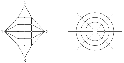
Figure 1: Specimens of planar fishnet graphs in position space with different boundary conditions. Bulk points stand for quartic integration points, $\int d^{4}x/\pi^{2}$, while edges are massless propagators, $1/(x-y)^{2}$. For the fishnet four-point functions considered in this paper, the $m$ vertical and $n$ horizontal external legs end on four fixed spacetime points $x_{1,2,3,4}$, as shown in the left panel ($m$ lines end on $x_{3,4}$; $n$ lines end on $x_{1,2}$). In the right panel, we show an $m$-by-$n$ fishnet graph with periodic boundary conditions in the angular direction. Such graphs are expected to scale as $\sim g_{c}^{-2mn}$ when $m,n\rightarrow\infty$, with $g_{c}$ a numerical constant Zamolodchikov:1980mb . The four-point function considered in this paper (left panel) scales differently, with a free energy per vertex that depends on the aspect ratio $k=n/m$.

This paper is structured as follows. In section 2, we analyze the integrability-based representations for the fishnet integrals and prove their equivalence with the determinant of ladder integrals. Our analysis relies on exact methods which may be applicable to more general fishnet graphs. We proceed with the analysis of the thermodynamic limit in section 3. Applying the saddle-point method to the matrix-model integrals gives us first order differential equations for the free-energy density, which can be solved simultaneously in terms of complete elliptic functions. We compare the obtained expression with a direct numerical evaluation of the determinant and study particular limits analytically. We conclude with a brief discussion of the dependence of the free energy on the boundary conditions. In section 4 we consider a more general scaling which combines the thermodynamic and short-distance limits and unveils a connection with the singular equation describing a classical spinning string in $AdS_{3}\times S^{1}$. Section 5 contains concluding remarks.

2 Integral representations

The fabric of the fishnet graphs – the conformal fishnet theory – is a theory of two $N_{c}\times N_{c}$ matrices of complex scalar fields $\phi_{1,2}$ and a quartic interaction, with (Euclidean) Lagrangian density Gurdogan:2015csr ; Caetano:2016ydc ; Grabner:2017pgm

$$\mathcal{L}=\textrm{Tr}\,\big{\{}\partial_{\mu}\phi_{i}\partial_{\mu}\phi^{\dagger}_{i}-(4\pi g)^{2}\phi_{1}\phi_{2}\phi_{1}^{\dagger}\phi_{2}^{\dagger}\big{\}}\,,$$ (1)

with the trace running over the “colour” indices and with $g^{2}$ a marginal coupling constant, which is kept fixed in the large $N_{c}$ limit Grabner:2017pgm ; Sieg:2016vap .

The fishnet four-point function of interest is defined as the leading colour-ordered contribution to the correlator

$$G_{m,n}(\{x_{i}\})=\langle\textrm{Tr}\{\phi_{2}^{n}(x_{1})\phi_{1}^{m}(x_{3})\phi_{2}^{\dagger n}(x_{2})\phi_{1}^{\dagger m}(x_{4})\}\rangle\,,$$ (2)

with the trace embracing all the fields. It receives a single contribution at large $N_{c}$, which is given by the $mn$-loop Feynman diagram shown in figure 2.

The graph is both ultraviolet (UV) and infrared (IR) finite, for generic $x_{1,2,3,4}$. Dropping a colour factor and stripping off overall weights, one has

$$G_{m,n}(\{x_{i}\})=\frac{g^{2mn}}{(x_{12}^{2})^{n}(x_{34}^{2})^{m}}\times\Phi_{m,n}(u,v)\,,$$ (3)

with $x_{ij}^{2}\equiv(x_{i}-x_{j})^{2}$, where $\Phi_{m,n}$ is a coupling-independent function of the two conformal cross ratios

$$u=\frac{x_{14}^{2}x_{23}^{2}}{x_{12}^{2}x_{34}^{2}}\equiv\frac{z\bar{z}}{(1-z)(1-\bar{z})},\qquad v=\frac{x_{13}^{2}x_{24}^{2}}{x_{12}^{2}x_{34}^{2}}\equiv\frac{u}{z\bar{z}}\,,$$ (4)

parametrized here in terms of two numbers $z,\bar{z}$. The latter are complex conjugates in Euclidean spacetime signature, and are treated as independent real numbers in the Minkowskian case.

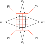
Figure 2: A transformation maps the space-time integral into a momentum space amplitude, shown in red lines, with external massive momenta $p_{1}=x_{23},p_{2}=x_{31},p_{3}=x_{14}$ and $p_{4}=x_{42}$, and with massless internal lines. The latter amplitude is subject to important analyticity requirements such as the Steinmann relations.

A representation for $\Phi_{m,n}$ was proposed in ref. Basso:2017jwq using integrability and analyticity. The proposal is that for $n\geqslant m$

$$\Phi_{m,n}=\left[\frac{(1-z)(1-\bar{z})}{z-\bar{z}}\right]^{m}I_{m,n}(z,\bar{z})\,,$$ (5)

where $I_{m,n}(z,\bar{z})$ is a pure function of weight $m\times n$ given by the determinant of an $m\times m$ Hankel matrix of ladder functions. It reads

$$I_{m,n}=\frac{1}{\mathcal{N}}\det_{1\leqslant i,j\leqslant m}(M_{i+j+n-m-1})\,,$$ (6)

with the matrix element

$$M_{p}=p!(p-1)!L_{p}(z,\bar{z})\,,$$ (7)

and normalization factor

$$\mathcal{N}=\prod_{k=0}^{2m-1}(n-m+k)!\,.$$ (8)

The particular case $m=1$ coincides with the well-known ladder integral $L_{p}(z,\bar{z})$, defined for a number of rungs $p\geqslant 0$ by Usyukina:1993ch ; Broadhurst:2010ds

$$L_{p}(z,\bar{z})=\begin{dcases}\sum_{j=p}^{2p}\frac{j![-\log{(z\bar{z})}]^{2p-j}}{p!(j-p)!(2p-j)!}[\text{Li}_{j}(z)-\text{Li}_{j}(\bar{z})]&\text{if}\ p\geqslant 1,\\ \frac{z-\bar{z}}{(1-z)(1-\bar{z})}&\text{if}\ p=0,\end{dcases}$$ (9)

with $\textrm{Li}_{j}(z)$ the polylogarithm of weight $j$,

$$\text{Li}_{j}(z)=\frac{z}{(j-1)!}\int\limits_{0}^{\infty}\mathrm{d}r\frac{r^{j-1}}{e^{r}-z}=\sum_{k=1}^{\infty}\frac{z^{k}}{k^{j}}\,,$$ (10)

where the Taylor series converges for $|z|<1$.

The determinant formula (6), when interpreted as the result for a scattering amplitude rather than a correlation function, nicely satisfies the Steinmann relations Steinmann ; Steinmann2 , which forbid sequential discontinuities in overlapping channels. In figure 2, the red lines indicate the scattering interpretation, and the two channels are $(p_{1}+p_{2})^{2}=x_{12}^{2}$ and $(p_{2}+p_{3})^{2}=x_{34}^{2}$. The Steinmann relations imply that

$${\rm Disc}_{x_{12}^{2}}{\rm Disc}_{x_{34}^{2}}I_{m,n}=0,$$ (11)

in the region where $x_{12}^{2}$ and $x_{34}^{2}$ both vanish, which is the neighborhood of $z,\bar{z}\rightarrow 1$. Conformal invariance then translates eq. (11) into the vanishing of the double discontinuity in $(1-z)(1-\bar{z})$:

$${\rm Disc}_{1}{\rm Disc}_{1}I_{m,n}=0.$$ (12)

(For example, one can wrap $z$ around 1, and keep $\bar{z}$ fixed, or wrap both in the same direction.) The single discontinuity of the ladder integral (9) is Basso:2017jwq ; Bourjaily:2020wvq

$${\rm Disc}_{1}L_{p}=2\pi\mathbf{i}\frac{(-1)^{p}}{p!(p-1)!}\,\log(z/\bar{z})\,(\log z\log\bar{z})^{p-1}\,,$$ (13)

with $\mathbf{i}=\sqrt{-1}$. Since the single discontinuity contains only $\log z$ and $\log\bar{z}$, the double discontinuity of any ladder integral vanishes, $[{\rm Disc}_{1}]^{2}L_{p}=0$. Furthermore, the discontinuities of any two columns (or two rows) of the matrix $M_{p}$ defined in (7) are proportional, because

$${\rm Disc}_{1}M_{p+1}=(-\log z\log\bar{z})\,{\rm Disc}_{1}M_{p}\,,$$ (14)

which guarantees the vanishing of the double discontinuity of the determinant (6) Basso:2017jwq . (A more general solution to the Steinmann relations is given by the minors of a semi-infinite matrix of ladders, as found in the study of large-charge correlators in $\mathcal{N}=4$ SYM Coronado:2018cxj ; Coronado:2018ypq .)

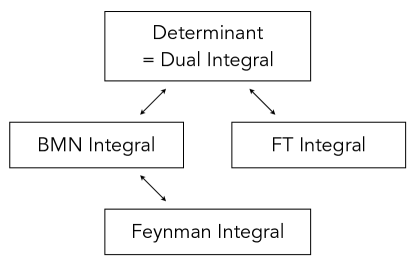
Figure 3: Representations of the fishnet four-point integral. The Feynman integral was recently proved to be equivalent to the BMN integral (26) in refs. Derkachov:2019tzo ; Derkachov:2020zvv . In this paper we concentrate on the pyramid at the top and derive the determinant formula from the BMN and FT integrability-based representations.

As alluded to before, along with the determinant (6), two matrix-model-like integrals, the BMN integral and FT integral, were given in ref. Basso:2017jwq . They originate from two different conjectural $\mathcal{N}=4$ SYM integrability-based tiling constructions, the “hexagonalization” Fleury:2016ykk ; Eden:2016xvg ; Fleury:2017eph ; Basso:2015zoa ; Basso:2018cvy and the “pentagon OPE” Basso:2013vsa ; Alday:2007mf ; Alday:2010ku . The former has been receiving a lot of attention recently, as it is closely related to the method of separation of variables for conformal integrable spin chains, which enabled the calculation of fishnet correlators in the 2d fishnet conformal field theories Derkachov:2018rot . This method was recently extended to four dimensions in refs. Derkachov:2019tzo ; Basso:2019xay ; Derkachov:2020zvv ; Chicherin:2012yn , allowing to put on firm ground the results obtained from the $\mathcal{N}=4$ SYM integrability-based tiling constructions. According to these analyses, the BMN representation discussed below is no longer a conjecture – it is proved to be equivalent to the Feynman integral. In this section we will close the remaining gaps to the determinant formula by proving its equivalence with both the BMN and FT integral representations, as schematized in figure 3.

2.1 Dual integral

To begin, let us recast the determinant formula (5) into an integral form which will prove very useful later on. Introducing the parametrization

$$z=-e^{\sigma+\varphi}\,,\qquad\bar{z}=-e^{\sigma-\varphi}\,,$$ (15)

we will show in this subsection that one may write the determinant in the form

$$\Phi_{m,n}=d(z,\bar{z})^{m}\times I^{{\rm Dual}}_{m,n}\,,$$ (16)

where $I^{{\rm Dual}}_{m,n}$ stands for the $m$-fold integral

$$I^{{\rm Dual}}_{m,n}=\frac{1}{2^{m}m!\mathcal{N}}\prod_{i=1}^{m}\int_{|\sigma|}^{\infty}\frac{\mathrm{d}x_{i}x_{i}(x_{i}^{2}-\sigma^{2})^{n-m}}{\cosh{\tfrac{1}{2}(x_{i}+\varphi)}\cosh{\tfrac{1}{2}(x_{i}-\varphi)}}\prod_{i<j}^{m}(x_{i}^{2}-x_{j}^{2})^{2}\,,$$ (17)

with $\mathcal{N}$ given in eq. (8), and with the kinematical prefactor

$$d(z,\bar{z})=\frac{(1-z)(1-\bar{z})}{\sqrt{z\bar{z}}}\,.$$ (18)

Note that this prefactor differs from the one in eq. (5), such that

$$I^{{\rm Dual}}_{m,n}=\left[\frac{\sqrt{z\bar{z}}}{z-\bar{z}}\right]^{m}I_{m,n}\,.$$ (19)

The representation (16) may be seen as a reduction of the more general functional determinant formulae obtained in refs. Kostov:2019stn ; Kostov:2019auq ; Belitsky:2019fan ; Belitsky:2020qrm ; Belitsky:2020qir ; Kostov:2021omc for large-charge correlators in $\mathcal{N}=4$ SYM theory, which resum infinite series of fishnet diagrams and generalizations thereof Coronado:2018ypq ; Coronado:2018cxj . In the following, we shall refer to eq. (17) as the “dual integral”, as it relates in our set-up to Fourier-like transforms of the integrability-based integrals to be studied later on.

The dual representation given in eqs. (16) and (17) holds for $\sigma\in\mathbb{R}$ and $\textrm{Im}\,\varphi\in(-\pi,\pi)$, which includes both the Minkowskian and the Euclidean kinematics, corresponding respectively to purely real and purely imaginary values of $\varphi$. It can be derived from the determinant (6) by first replacing the ladder functions by their integral representation Broadhurst:2010ds ; Kostov:2019stn ; Kostov:2019auq

$$L_{p}(z,\bar{z})=\frac{(z-\bar{z})}{2\sqrt{z\bar{z}}\,p!(p-1)!}\int\limits_{|\sigma|}^{\infty}\frac{\mathrm{d}xx(x^{2}-\sigma^{2})^{p-1}}{\cosh{\tfrac{1}{2}(x+\varphi)}\cosh{\tfrac{1}{2}(x-\varphi)}}\,.$$ (20)

This identity follows directly from the definition (10) of the polylogarithms. Namely, plugging eq. (10) into the sum in eq. (9), with $2\sigma=\log{(z\bar{z})}$, and relabelling $j\rightarrow 2p-j$, one finds

$$L_{p}(z,\bar{z}) =\sum_{j=0}^{p}\frac{(2p-j)!(-2\sigma)^{j}}{p!j!(p-j)!}[\text{Li}_{2p-j}(z)-\text{Li}_{2p-j}(\bar{z})]$$ (21)

$$=\frac{2}{p!(p-1)!}\int\limits_{0}^{\infty}\mathrm{d}r\,r^{p-1}(r-\sigma)(r-2\sigma)^{p-1}\bigg{[}\frac{z}{e^{r}-z}-\frac{\bar{z}}{e^{r}-\bar{z}}\bigg{]}$$

$$=\frac{(z-\bar{z})}{2\sqrt{z\bar{z}}\,p!(p-1)!}\int\limits_{-\sigma}^{\infty}\frac{\mathrm{d}xx(x^{2}-\sigma^{2})^{p-1}}{\cosh{\tfrac{1}{2}(x+\varphi)}\cosh{\tfrac{1}{2}(x-\varphi)}}\,,$$

making use of the combinatorial identity (for $p>0$)

$$\sum_{j=0}^{p}\frac{(p-1)!(2p-j)!}{j!(p-j)!(2p-j-1)!}r^{p-j}(-2\sigma)^{j}=2(r-\sigma)(r-2\sigma)^{p-1}\,,$$ (22)

and changing variables, $x=r-\sigma$. One recovers eq. (20) by manipulating the contour of integration, noting that the integrand is antisymmetric under $x\rightarrow-x$.

One then inserts eq. (20) inside the determinant in eq. (6) and applies the so-called Cauchy-Binet-Andréief formula (Lemma 1 in appendix A) to bring the determinant below the integral sign. Using eq. (19) to remove the factors of $(z-\bar{z})/\sqrt{z\bar{z}}$, one finds

$$I^{{\rm Dual}}_{m,n} =\frac{1}{2^{m}\mathcal{N}}\det_{1\leqslant i,j\leqslant m}\left[\int_{|\sigma|}^{\infty}\frac{\mathrm{d}xx(x^{2}-\sigma^{2})^{n-m+i+j-2}}{\cosh{\tfrac{1}{2}(x+\varphi)}\cosh{\tfrac{1}{2}(x-\varphi)}}\right]$$ (23)

$$=\frac{1}{2^{m}m!\mathcal{N}}\prod_{\ell=1}^{m}\int_{|\sigma|}^{\infty}\frac{\mathrm{d}x_{\ell}x_{\ell}(x_{\ell}^{2}-\sigma^{2})^{n-m}}{\cosh{\tfrac{1}{2}(x_{\ell}+\varphi)}\cosh{\tfrac{1}{2}(x_{\ell}-\varphi)}}[\Delta_{m}(x^{2})]^{2}\,.$$

One encounters two copies of the determinant

$$\Delta_{m}(x^{2})\equiv\det_{1\leqslant i,j\leqslant m}\Bigl{[}(x_{j}^{2}-\sigma^{2})^{i-1}\Bigr{]}\,,$$ (24)

which is actually independent of $\sigma$, and is the Vandermonde determinant

$$\Delta_{m}(x^{2})=\det_{1\leqslant i,j\leqslant m}(x_{j}^{2(i-1)})=\prod_{j>i}^{m}(x^{2}_{j}-x^{2}_{i})\,,$$ (25)

associated with the set $\{x_{j}^{2},j=1,\ldots,m\}$. Equation (23) proves the equivalence of the dual and original representations, eqs. (16) and (17).

2.2 BMN integral

The first integrability-based integral to be discussed is the BMN integral in ref. Basso:2017jwq . This representation yields the pure function $I_{m,n}$ in the form of a sum of integrals,

$$I^{\rm BMN}_{m,n} =\frac{1}{m!}\prod_{\ell=1}^{m}\operatorname*{\mathchoice{\ooalign{$\displaystyle\sum$\cr$\displaystyle\int$\cr}}{\ooalign{\raisebox{0.14pt}{\scalebox{0.7}{$\textstyle\sum$}}\cr$\textstyle\int$\cr}}{\ooalign{\raisebox{0.2pt}{\scalebox{0.6}{$\scriptstyle\sum$}}\cr$\scriptstyle\int$\cr}}{\ooalign{\raisebox{0.2pt}{\scalebox{0.6}{$\scriptstyle\sum$}}\cr$\scriptstyle\int$\cr}}}_{\ell}\frac{a_{\ell}\chi_{\ell}(z)}{(u_{\ell}^{2}+a_{\ell}^{2}/4)^{m+n}}\prod_{i<j}^{m}\left[(u_{i}-u_{j})^{2}+\tfrac{1}{4}(a_{i}-a_{j})^{2}\right]\left[(u_{i}-u_{j})^{2}+\tfrac{1}{4}(a_{i}+a_{j})^{2}\right]\,,$$ (26)

with $\operatorname*{\mathchoice{\ooalign{$\displaystyle\sum$\cr$\displaystyle\int$\cr}}{\ooalign{\raisebox{0.14pt}{\scalebox{0.7}{$\textstyle\sum$}}\cr$\textstyle\int$\cr}}{\ooalign{\raisebox{0.2pt}{\scalebox{0.6}{$\scriptstyle\sum$}}\cr$\scriptstyle\int$\cr}}{\ooalign{\raisebox{0.2pt}{\scalebox{0.6}{$\scriptstyle\sum$}}\cr$\scriptstyle\int$\cr}}}_{\ell}\equiv\sum_{a_{\ell}\geqslant 1}\int_{\mathbb{R}}\mathrm{d}u_{\ell}/(2\pi)$ and (with $\mathbf{i}=\sqrt{-1}$)

$$\chi_{\ell}(z)\equiv(z\bar{z})^{-\mathbf{i}u_{\ell}}\left((z/\bar{z})^{\frac{1}{2}a_{\ell}}-(\bar{z}/z)^{\frac{1}{2}a_{\ell}}\right)=2(-1)^{a_{\ell}}\sinh{(a_{\ell}\varphi)}e^{-2\mathbf{i}u_{\ell}\sigma}\,.$$ (27)

The translation to the variables $\sigma$ and $\varphi$ follows from eq. (15), after fixing the square-root ambiguity appropriately. The representation (26) is initially defined in Euclidean kinematics, that is, for $\sigma\in\mathbb{R}$ and $-\mathbf{i}\varphi\in(-\pi,\pi)$, and then analytically continued. Its direct evaluation is straightforward for low values of $m$ and the result is seen to reproduce the ladder determinant. In particular, one easily verifies the agreement with the ladder series Fleury:2016ykk ,

$$L_{n}(z,\bar{z})=\sum_{a_{1}=1}^{\infty}\int\frac{du_{1}}{2\pi}\frac{a_{1}\chi_{1}(z)}{(u^{2}_{1}+\frac{a^{2}_{1}}{4})^{n+1}}\,,$$ (28)

when $m=1$. In this subsection, we shall prove the general identity

$$I^{\rm BMN}_{m,n}=\left[\frac{z-\bar{z}}{\sqrt{z\bar{z}}}\right]^{m}I^{\rm Dual}_{m,n}=(e^{-\varphi}-e^{\varphi})^{m}I^{\rm Dual}_{m,n}\,,$$ (29)

with $I^{\rm Dual}_{m,n}$ the integral form of the determinant (17), for all $m$ and $n$, with $n\geqslant m$.

To begin, we note that the bulk of the integrand in eq. (26) can be written concisely as a Vandermonde determinant. Namely, defining conjugate variables

$$\xi_{2\ell-1}=u_{\ell}+\mathbf{i}a_{\ell}/2\,,\qquad\xi_{2\ell}=u_{\ell}-\mathbf{i}a_{\ell}/2\,,\qquad\ell=1,\ldots,m\,,$$ (30)

one immediately finds that the integrand can be cast into the compact form

$$I^{\rm BMN}_{m,n}=\frac{\mathbf{i}^{m}}{m!}\prod_{\ell=1}^{m}\operatorname*{\mathchoice{\ooalign{$\displaystyle\sum$\cr$\displaystyle\int$\cr}}{\ooalign{\raisebox{0.14pt}{\scalebox{0.7}{$\textstyle\sum$}}\cr$\textstyle\int$\cr}}{\ooalign{\raisebox{0.2pt}{\scalebox{0.6}{$\scriptstyle\sum$}}\cr$\scriptstyle\int$\cr}}{\ooalign{\raisebox{0.2pt}{\scalebox{0.6}{$\scriptstyle\sum$}}\cr$\scriptstyle\int$\cr}}}_{\ell}\frac{\chi_{\ell}(z)}{(\xi_{2\ell-1}\xi_{2\ell})^{m+n}}\times\Delta_{2m}(\xi)\,,$$ (31)

where $\Delta_{2m}(\xi)$ is the Vandermonde determinant for the set $\{\xi_{1},\xi_{2},\ldots,\xi_{2m}\}$,

$$\Delta_{2m}(\xi) =\det\,(\xi_{j}^{i-1})=\prod_{j>i}^{2m}(\xi_{j}-\xi_{i})$$ (32)

$$=\prod_{i=1}^{m}(-\mathbf{i}a_{i})\times\prod_{i>j}^{m}\left[(u_{i}-u_{j})^{2}+\tfrac{1}{4}(a_{i}-a_{j})^{2}\right]\left[(u_{i}-u_{j})^{2}+\tfrac{1}{4}(a_{i}+a_{j})^{2}\right]\,.$$

One can make immediate use of this remarkable simplification to disentangle pairs of $\xi$ variables and cast the integral in the form of the Pfaffian of a $2m\times 2m$ skew-symmetric matrix $B$,

$$I^{\rm BMN}_{m,n}=\mathbf{i}^{m}\textrm{pf}\,B=\frac{\mathbf{i}^{m}}{2^{m}m!}\sum_{\pi\in S_{2m}}{\rm sign}{(\pi)}\prod_{\ell=1}^{m}B_{\pi(2\ell-1),\pi(2\ell)}\,,$$ (33)

with the sum running over the permutations of the set $\{1,\ldots,2m\}$, by plugging

$$\Delta_{2m}(\xi)=\sum_{\pi\in S_{2m}}{\rm sign}{(\pi)}\prod_{\ell=1}^{m}(\xi_{2\ell-1}^{\pi(2\ell-1)-1}\xi_{2\ell}^{\pi(2\ell)-1})$$ (34)

into eq. (32), and defining

$$B_{ij}=\operatorname*{\mathchoice{\ooalign{$\displaystyle\sum$\cr$\displaystyle\int$\cr}}{\ooalign{\raisebox{0.14pt}{\scalebox{0.7}{$\textstyle\sum$}}\cr$\textstyle\int$\cr}}{\ooalign{\raisebox{0.2pt}{\scalebox{0.6}{$\scriptstyle\sum$}}\cr$\scriptstyle\int$\cr}}{\ooalign{\raisebox{0.2pt}{\scalebox{0.6}{$\scriptstyle\sum$}}\cr$\scriptstyle\int$\cr}}}_{\ell}\frac{\chi_{\ell}(z)}{(\xi_{2\ell-1}\xi_{2\ell})^{m+n}}(\xi_{2\ell-1}^{i-1}\xi_{2\ell}^{j-1}-\xi_{2\ell-1}^{j-1}\xi_{2\ell}^{i-1})\,.$$ (35)

A drawback is that the elements $B_{ij}(z,\bar{z})$ are not ladders, for $j\neq i\pm 1$, but derivatives thereof. Further non-trivial algebraic identities are needed to “purify” the expression and reduce the integral to a determinant of an $m\times m$ matrix, as discussed in refs. Kostov:2019stn ; Kostov:2019auq ; Belitsky:2019fan ; Belitsky:2020qrm ; Belitsky:2020qir ; Kostov:2021omc in the related context of large-charge correlators in $\mathcal{N}=4$ SYM.

Interestingly, it turns out to be possible to bypass this difficulty by decoupling all $\xi$ variables from the onset. (This promotes the full permutation symmetry of the integrand to the integral level, if not for the contours, see below.) The preliminary step is to relax the constraints $\mathbf{i}(\xi_{2\ell}-\xi_{2\ell-1})=a_{\ell}\in\mathbb{N}$ among conjugate variables (30), by turning the sums over positive $a$’s into integrals. This task may be done efficiently with the help of the Mellin-Barnes summation technique. The key formula is Lemma 2 in appendix A. It reads

$$\sum_{a=1}^{\infty}(-1)^{a}(e^{a\varphi}-e^{-a\varphi})f(a)=\int\limits_{-\infty}^{\infty}\mathrm{d}x\left[\frac{1}{e^{\varphi-x}+1}-\frac{1}{e^{-\varphi-x}+1}\right]\,\int_{\mathcal{C}}\frac{\mathrm{d}a}{2\pi\mathbf{i}}f(a)e^{-ax}\,,$$ (37)

for any suitably smooth function $f$ and with $\mathcal{C}$ parallel to the imaginary axis, $\mathcal{C}=\varepsilon+\mathbf{i}\mathbb{R}$ with $\varepsilon\in\left(0,1\right)$. This representation stems from the combination of the Sommerfeld-Watson transform,

$$\sum_{a=1}^{\infty}(-1)^{a}(e^{a\varphi}-e^{-a\varphi})f(a) =\mathbf{i}\int_{\varepsilon-\mathbf{i}\infty}^{\varepsilon+\mathbf{i}\infty}\mathrm{d}a\frac{\sinh{(a\varphi)}}{\sin{(a\pi)}}f(a)\,,$$ (38)

with an integral transform for the inverse sine factor, see eq. (195) in appendix A. This combination is well-suited to our problem as it puts in place the dual variable $x$ entering the integral form of the ladder determinant. It also removes the constraints on $\varphi$, which may now be chosen anywhere inside the extended kinematics $\textrm{Im}\,\varphi\in(-\pi,\pi)$. Applying eq. (37) to each sum in eq. (31), we get

$$I^{\rm BMN}_{m,n} =\frac{(-\mathbf{i})^{m}}{2^{m}m!}\int_{\mathbb{R}^{m}}\prod_{\ell=1}^{m}\frac{\mathrm{d}x_{\ell}(e^{\varphi}-e^{-\varphi})}{2\cosh{\frac{1}{2}(x_{\ell}+\varphi)}\cosh{\frac{1}{2}(x_{\ell}-\varphi)}}\,\mathcal{I}_{1}(\sigma,\{x\})\,,$$ (39)

with all dependence on $\sigma$ factorizing neatly into the integral

$$\mathcal{I}_{1}(\sigma,\{x\})=\prod_{\ell=1}^{m}\int_{\mathcal{C}}\frac{\mathrm{d}a_{\ell}}{2\pi\mathbf{i}}\int_{\mathbb{R}}\frac{\mathrm{d}u_{\ell}}{2\pi}\frac{e^{-a_{\ell}x_{\ell}-2\mathbf{i}u_{\ell}\sigma}}{(\xi_{2\ell-1}\xi_{2\ell})^{m+n}}\times\Delta_{2m}(\xi)\,.$$ (40)

The key simplification is that $\xi_{2\ell-1}$ and $\xi_{2\ell}$ can now be regarded as independent variables. They would be real for $u_{\ell}\in\mathbb{R}$ and $a_{\ell}\in\mathbf{i}\mathbb{R}$. Instead, they run here parallel to the real axis, along the contours

$$\xi_{2\ell-1}\in\Gamma_{+}\equiv\mathbb{R}+\mathbf{i}\varepsilon\,,\qquad\xi_{2\ell}\in\Gamma_{-}\equiv\mathbb{R}-\mathbf{i}\varepsilon\,,$$ (41)

because $a_{\ell}$ has a small positive real part $\varepsilon$. Hence,

$$\int_{\mathcal{C}}\frac{\mathrm{d}a_{\ell}}{2\pi\mathbf{i}}\int_{\mathbb{R}}\frac{\mathrm{d}u_{\ell}}{2\pi}=\int_{\Gamma_{+}\times\Gamma_{-}}\frac{\mathrm{d}\xi_{2\ell-1}\mathrm{d}\xi_{2\ell}}{(2\pi\mathbf{i})^{2}}\,,\qquad\forall\ell=1,\ldots,m\,,$$ (42)

after taking into account the Jacobian ($=-\mathbf{i}$) for the change of variables (30). We may now write $\mathcal{I}_{1}(\sigma,\{x\})$ as a bunch of decoupled $\xi$-integrals using eq. (34) and recast it as the determinant of a $2m\times 2m$ matrix $A$,

$$\mathcal{I}_{1}(\sigma,\{x\})=\det\,A\,,$$ (43)

with elements,

$$A_{k,2\ell-1}=A^{+}_{k}(x_{\ell})\,,\qquad A_{k,2\ell}=A^{-}_{k}(x_{\ell})\,,\qquad k=1,\ldots,2m,\,\,\,\ell=1,\ldots,m\,,$$ (44)

and

$$A^{\pm}_{k}(x)\equiv\int_{\Gamma_{\pm}}\frac{\mathrm{d}\xi}{2\pi\mathbf{i}}\xi^{k-m-n-1}e^{\mathbf{i}(\pm x-\sigma)\xi}\,.$$ (45)

Closing the contour of integration in the upper/lower half $\xi$ plane, depending on whether $\pm x-\sigma\gtrless 0$, one finds

$$A^{\pm}_{k}(x)= \mp\frac{1}{(m+n-k)!}[\mathbf{i}(\pm x-\sigma)]^{m+n-k}\theta(-x\pm\sigma)\,,$$ (46)

with $\theta(t)$ the Heaviside step function, $\theta(t)=1$ for $t\geqslant 0$ and $\theta(t)=0$ otherwise.

One proceeds with straightforward linear algebra. Plugging (46) into eq. (43), we first factor out $\mp[\mathbf{i}(\pm x_{\ell}-\sigma)]^{n-m}\theta(-x_{\ell}\pm\sigma)$, column by column, and then $1/(m+n-k)!$, row by row. The leftover factor is a Vandermonde determinant for the set $\{\mathbf{i}(x_{1}-\sigma),\mathbf{i}(-x_{1}-\sigma),\mathbf{i}(x_{2}-\sigma),\mathbf{i}(-x_{2}-\sigma),\dots,\mathbf{i}(x_{m}-\sigma),\mathbf{i}(-x_{m}-\sigma)\}$. As such, it does not depend on $\sigma$ and can be written concisely as

$$(-\mathbf{i})^{m}\prod_{i<j}^{m}(x_{i}-x_{j})^{2}\prod_{i,j}^{m}(x_{i}+x_{j})=(-\mathbf{i})^{m}\prod_{i=1}^{m}2x_{i}\times[\Delta_{m}(x^{2})]^{2}\,.$$ (47)

Assembling all factors together, we obtain

$$\mathcal{I}_{1}(\sigma) =\frac{\mathbf{i}^{m}}{\mathcal{N}}\prod_{i=1}^{m}\theta(-|\sigma|-x_{i})2x_{i}(x_{i}^{2}-\sigma^{2})^{n-m}\times[\Delta_{m}(x^{2})]^{2}\,,$$ (48)

and, therefore,

$$I^{\rm BMN}_{m,n}=\frac{(e^{\varphi}-e^{-\varphi})^{m}}{2^{m}m!\mathcal{N}}\prod_{i=1}^{m}\int_{-\infty}^{-|\sigma|}\frac{\mathrm{d}x_{i}x_{i}(x_{i}^{2}-\sigma^{2})^{n-m}}{\cosh{\frac{1}{2}(\varphi+x_{i})}\cosh{\frac{1}{2}(\varphi-x_{i})}}[\Delta_{m}(x^{2})]^{2}\,,$$ (49)

which implies eq. (29) with eq. (23) and concludes the proof that the BMN integral (26) is equivalent to the determinant formula (6).

It is worth mentioning that the above analysis would also apply to the anisotropic fishnet diagrams Zamolodchikov:1980mb ; Kazakov:2018qbr associated with a theory in which the two scalar fields are given non-canonical dimensions $1\mp 2\omega$, with $\omega\in[0,1/2)$ playing the role of an anisotropy parameter. The equivalent of the “BMN representation” for the $m\times n$ deformed fishnet diagram in four dimensions was worked out in refs. Derkachov:2019tzo ; Derkachov:2020zvv , along with other generalizations of the correlator, using the method of separation of variables. It was found to take the same form as for isotropic fishnets, that is (26), up to the replacement

$$\frac{1}{(u_{\ell}^{2}+a_{\ell}^{2}/4)^{m+n}}\rightarrow[f(\tfrac{a_{\ell}}{2}-\mathbf{i}u_{\ell})f(\tfrac{a_{\ell}}{2}+\mathbf{i}u_{\ell})]^{m+n},$$ (50)

with $f(y)=\Gamma(y+\omega)/\Gamma(y+1-\omega)$ and with $\Gamma$ the Euler Gamma function. Importantly, since the $\xi$-integrals stay factorized under this deformation, one can repeat the above analysis and derive a $2m\times 2m$ determinant representation for the correlator by slightly modifying the integrals in eq. (45), using

$$A_{k}^{\pm}(x)\rightarrow\int_{\Gamma_{\pm}}\frac{d\xi}{2\pi\mathbf{i}}\xi^{k-1}[\mp\mathbf{i}f(\mp\mathbf{i}\xi)]^{m+n}e^{\mathbf{i}(\pm x-\sigma)\xi}\,.$$ (51)

It is not clear, however, if the result may be further simplified and cast into the form of a determinant of an $m\times m$ matrix, as in the undeformed case, since the factorization of the determinant observed in eq. (48) depends very much on the explicit form of the $\xi$-integrals. In contrast, 2d fishnet correlators were found Derkachov:2018rot to admit a uniform $m\times m$ determinant representation for all values of the anisotropy parameter.

2.3 FT integral

The second integrability-based representation is the so-called flux-tube representation. It arises in the Minkowskian kinematics when one considers the correlator as sitting inside a null conformal frame, as depicted in figure 4. The end-points of the correlator are then interpreted as producing beams of flux-tube particles at the positions

$$z=-e^{2\sigma_{1}}=-e^{\varphi+\sigma}\,,\qquad\bar{z}=-e^{-2\sigma_{2}}=-e^{\sigma-\varphi}\,,$$ (52)

with $\sigma_{1,2}\in\mathbb{R}$, along two orthogonal lightcone directions, $n^{2}=\bar{n}^{2}=0$, $n\cdot\bar{n}=1$, as explained in the caption of figure 4.

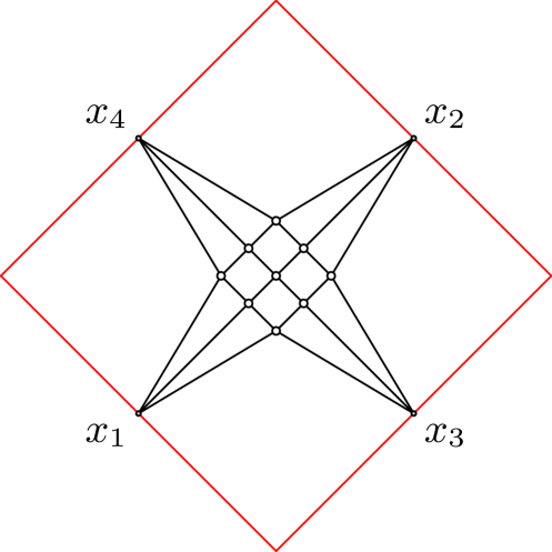
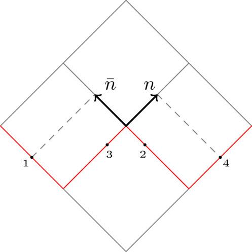
Figure 4: The flux-tube factorization relies on lightcone coordinates to parametrize the positions of the four points $x_{1,2,3,4}$ along a null conformal frame (square). In the case of interest, i.e. for spacelike separations, $x_{ij}^{2}<0$, the null square is the Poincaré patch of (conformally compactified) $\mathbb{R}^{1,1}\subset\mathbb{R}^{1,3}$, as shown in the right panel. Two points are placed at the boundary of the patch, with $n\cdot x_{1}=\bar{n}\cdot x_{4}=1$ and $n,\bar{n}$ two orthogonal lightlike vectors, $n^{2}=\bar{n}^{2}=0$, $n\cdot\bar{n}=1$. The remaining points are sitting at $n\cdot x_{2}=z$ and $\bar{n}\cdot x_{3}=\bar{z}$, with $z,\bar{z}$ both real and negative.

A nice feature of the flux-tube representation is that it treats symmetrically the $m$ and $n$ lines of the fishnet graph. Each set of lines is assigned to a set of rapidities, $\{u_{i=1,\ldots,m}\}$ and $\{v_{j=1,\ldots,n}\}$, representing the momenta of the flux-tube excitations, moving across the conformal square, and conjugate to the coordinates (52). The price to pay is that it gives rise to more complicated integrals involving both rational and hyperbolic functions. As explained in ref. Basso:2017jwq , in this representation, the correlator takes the form

$$\Phi_{m,n} =d(z,\bar{z})^{m}\times\pi^{\frac{1}{2}(m+n)(m+n+1)}(2\cosh\sigma_{2})^{n-m}\times I^{\rm FT}_{m,n}\,,$$ (53)

where $I^{\rm FT}_{m,n}$ is the $m\times n$ Fourier integral

$$\begin{split}&I^{\rm FT}_{m,n}=\int\limits_{\mathbb{R}^{m}}\frac{\mathrm{d}\bm{u}}{m!}\int\limits_{\mathbb{R}^{n}}\frac{\mathrm{d}\bm{v}}{n!}\prod_{i=1}^{m}\frac{e^{2\mathbf{i}u_{i}\sigma_{1}}}{\cosh{(\pi u_{i})}}\prod_{j=1}^{n}\frac{e^{2\mathbf{i}v_{j}\sigma_{2}}}{\cosh{(\pi v_{j})}}\\ &\qquad\qquad\times\Delta_{m}(u)\Delta_{m}(\tanh{(\pi u)})\Delta_{n}(v)\Delta_{n}(\tanh{(\pi v)})\prod_{i,j}^{m,n}\frac{\tanh{(\pi u_{i})}-\tanh{(\pi v_{j})}}{u_{i}-v_{j}}\,,\end{split}$$ (54)

with $\mathrm{d}\bm{u}=\prod_{i=1}^{m}du_{i}/(2\pi),\mathrm{d}\bm{v}=\prod_{j=1}^{n}dv_{j}/(2\pi),$ and with the $\Delta$’s referring as before to Vandermonde determinants,

$$\Delta_{m}(u)=\prod_{j>i}^{m}(u_{j}-u_{i})\,,\qquad\Delta_{m}(\tanh{(\pi u)})=\prod_{j>i}^{m}(\tanh{(\pi u_{j}})-\tanh{(\pi u_{i})})\,,$$ (55)

and similarly for the $v$’s. Integrals of this type were discussed in refs. Derkachov:2016dhc ; Derkachov:2019ynh ; Derkachov:2020zvv in connection with the separation of variables for $SL(2,\mathbb{R})$ spin chains. In particular, in the cases where $m=0$ or $n=0$, the integral matches with the norm of the separated wave function, and it can be evaluated straightforwardly using eq. (54) of ref. Derkachov:2016dhc . Below we explain how to calculate the integral in the general case, $m,n\neq 0$.

The mixing among hyperbolic and rational interactions makes the flux-tube integral harder to treat than the BMN one. The problem can be circumvented, however, by collecting these two types of interactions into suitable determinants.

The rational part, for instance, can be encoded in a generalized Cauchy determinant Han:2000rec ,

$$\frac{\Delta_{m}(u)\Delta_{n}(v)}{\prod_{i,j}(u_{i}-v_{j})}=(-1)^{\frac{1}{2}m(2n-m-1)}\times\det_{n}C\,,$$ (56)

where $C$ is a “centaur” $n\times n$ matrix, mixing Cauchy and Vandermonde entries, defined for $n\geqslant m$ and two sets of variables $\{u_{1},\ldots,u_{m}\}$ and $\{v_{1},\ldots,v_{n}\}$ by

$$C=\left(\phantom{\begin{matrix}\dfrac{1}{u_{1}-v_{n}}\vspace{0.5em}\\ \dfrac{1}{u_{2}-v_{n}}\\ \vdots\\ \dfrac{1}{u_{m}-v_{n}}\\ \\ \\ 1\\ v_{n}\\ \vdots\\ v_{n}^{n-m-1}\end{matrix}}\right.\begin{matrix}\dfrac{1}{u_{1}-v_{1}}&\dfrac{1}{u_{1}-v_{2}}&\cdots&\dfrac{1}{u_{1}-v_{n}}\vspace{0.5em}\\ \dfrac{1}{u_{2}-v_{1}}&\dfrac{1}{u_{2}-v_{2}}&\cdots&\dfrac{1}{u_{2}-v_{n}}\\ \vdots&\vdots&\vdots&\vdots\\ \dfrac{1}{u_{m}-v_{1}}&\dfrac{1}{u_{m}-v_{2}}&\cdots&\dfrac{1}{u_{m}-v_{n}}\\ &&&\vspace{-0.5em}\\ \hline\cr\vspace{-1em}\\ 1&1&\cdots&1\\ v_{1}&v_{2}&\cdots&v_{n}\\ \vdots&\vdots&\vdots&\vdots\\ v_{1}^{n-m-1}&v_{2}^{n-m-1}&\cdots&v_{n}^{n-m-1}\end{matrix}\left.\phantom{\begin{matrix}\dfrac{1}{u_{1}-v_{n}}\vspace{0.5em}\\ \dfrac{1}{u_{2}-v_{n}}\\ \vdots\\ \dfrac{1}{u_{m}-v_{n}}\\ \\ \\ 1\\ v_{n}\\ \vdots\\ v_{n}^{n-m-1}\end{matrix}}\right)\begin{tabular}[]{l}$\left.\hbox to0.0pt{$\displaystyle\phantom{\begin{matrix}\dfrac{1}{u_{1}-v_{n}}\vspace{0.5em}\\ \dfrac{1}{u_{2}-v_{n}}\\ \vdots\\ \dfrac{1}{u_{m}-v_{n}}\\ \hline\cr\vspace{-1em}\\ \leavevmode\nobreak\ \ \end{matrix}}$\hss}\right\}m$\\ $\left.\hbox to0.0pt{$\displaystyle\phantom{\begin{matrix}1\\ v_{n}\\ \vdots\\ v_{n}^{n-m-1}\\ \leavevmode\nobreak\ \ \end{matrix}}$\hss}\right\}n-m$\end{tabular}\,.$$ (57)

The hyperbolic factors, on the other hand, can be seen as coming from the action of the Vandermonde differential operator

$$\Delta_{m+n}(\{\overrightarrow{\partial_{v_{j}}},\overrightarrow{\partial_{u_{i}}}\})\equiv\prod_{i>j}^{m}(\partial_{u_{j}}-\partial_{u_{i}})\prod_{i>j}^{n}(\partial_{v_{j}}-\partial_{v_{i}})\prod_{i,j}^{n,m}(\partial_{v_{j}}-\partial_{u_{i}})$$ (58)

on the factor $\prod_{i,j}\operatorname{sech}({\pi u_{i})}\operatorname{sech}{(\pi v_{j})}$, as shown in appendix A (Lemma 4). Accordingly, the integral can be written more concisely as

$$I^{\rm FT}_{m,n} =\frac{(-1)^{\frac{1}{2}m(2n-m-1)}}{\prod_{j=1}^{m+n}(j-1)!}\left(\frac{-1}{\pi}\right)^{\frac{1}{2}(m+n)(m+n-1)}$$ (59)

$$\times\int_{\mathbb{R}^{m}}\frac{\mathrm{d}\bm{u}}{m!}\int_{\mathbb{R}^{n}}\frac{\mathrm{d}\bm{v}}{n!}\prod_{i=1}^{m}e^{2\mathbf{i}u_{i}\sigma_{1}}\prod_{j=1}^{n}e^{2\mathbf{i}v_{j}\sigma_{2}}\times\det\limits_{n}C\times\Delta_{m+n}(\{\overrightarrow{\partial_{v_{j}}},\overrightarrow{\partial_{u_{i}}}\})\prod_{i,j}\operatorname{sech}({\pi u_{i})}\operatorname{sech}{(\pi v_{j})}\,.$$

We may then perform an integration by parts, using

$$\Delta_{m+n}(\{\overrightarrow{\partial_{v_{j}}},\overrightarrow{\partial_{u_{i}}}\})=\Delta_{m+n}(\{-\overleftarrow{\partial_{v_{j}}},-\overleftarrow{\partial_{u_{i}}}\})=(-1)^{\frac{1}{2}(m+n)(m+n-1)}\Delta_{m+n}(\{\overleftarrow{\partial_{v_{j}}},\overleftarrow{\partial_{u_{i}}}\})\,,$$ (60)

with the arrows indicating on which side of the integrand in eq. (59) the derivative is acting. Note that there are no boundary terms, since the integrand is exponentially small at infinity. Using the Leibniz formula for multi-linear forms,

$$\Delta_{m+n}(\{\overrightarrow{\partial_{v_{j}}},\overrightarrow{\partial_{u_{i}}}\})\bigg{[}e^{2\mathbf{i}\sum_{i}u_{i}\sigma_{1}+2\mathbf{i}\sum_{j}v_{j}\sigma_{2}}\mathcal{F}(\{u_{i},v_{j}\})\bigg{]}$$ (61)

$$\qquad\qquad=e^{2\mathbf{i}\sum_{i}u_{i}\sigma_{1}+2\mathbf{i}\sum_{j}v_{j}\sigma_{2}}\Delta_{m+n}(\{\overrightarrow{\partial_{v_{j}}}+2\mathbf{i}\sigma_{2},\overrightarrow{\partial_{u_{i}}}+2\mathbf{i}\sigma_{1}\})\mathcal{F}(\{u_{i},v_{j}\})\,,$$

which applies to any function $\mathcal{F}(\{u_{i},v_{j}\})$, we get

$$I^{\rm FT}_{m,n} =\frac{(-1)^{\frac{1}{2}m(2n-m-1)}}{\prod_{j=1}^{m+n}(j-1)!}\left(\frac{1}{\pi}\right)^{\frac{1}{2}(m+n)(m+n-1)}$$ (62)

$$\times\int_{\mathbb{R}^{m}}\frac{\mathrm{d}\bm{u}}{m!}\int_{\mathbb{R}^{n}}\frac{\mathrm{d}\bm{v}}{n!}\prod_{i=1}^{m}\frac{e^{2\mathbf{i}u_{i}\sigma_{1}}}{\cosh{(\pi u_{i})}}\prod_{j=1}^{n}\frac{e^{2\mathbf{i}v_{j}\sigma_{2}}}{\cosh{(\pi v_{j})}}\times\Delta_{m+n}(\{\overrightarrow{\partial_{v_{j}}}+2\mathbf{i}\sigma_{2},\overrightarrow{\partial_{u_{i}}}+2\mathbf{i}\sigma_{1}\})\det_{n}C\,.$$

The next step is to disentangle the integrals in $\{u_{i}\}$ and $\{v_{j}\}$. We may do so by exponentiating the first $m$ lines of the matrix $C$ using Schwinger’s trick,

$$\frac{1}{u-v}=-\mathbf{i}\int_{0}^{\infty}\mathrm{d}r\,e^{\mathbf{i}r(u-v+\mathbf{i}0)}\,,$$ (63)

with $\mathbf{i}0$’s introduced to ensure convergence. We shall omit the latter prescription in the following, since the integrand is regular when $u_{i}=v_{j},\forall i,j$. Factoring out $e^{\mathbf{i}r_{i}u_{i}}$, row by row, we get

$$\det_{n}C=(-\mathbf{i})^{m}\int_{\mathbb{R}^{m}_{+}}\mathrm{d}\vec{r}\,e^{\mathbf{i}\sum_{i}r_{i}u_{i}}\det_{n}\tilde{C}\,,$$ (64)

with $\mathrm{d}\vec{r}=\prod_{i=1}^{m}\mathrm{d}r_{i}$, $\mathbb{R}_{+}=(0,\infty)$, and where the matrix $\tilde{C}$ has the same structure as $C$ up to the replacement $1/(u_{i}-v_{j})\to e^{-\mathbf{i}r_{i}v_{j}}$. Plugging (64) into (62) and applying the Leibniz formula to the phases in eq. (64) allow us to strip off the $\{u_{i}\}$ dependence,

$$I^{\rm FT}_{m,n} =\frac{(-\mathbf{i})^{m(2n-m)}}{\prod_{j=1}^{m+n}(j-1)!}\left(\frac{1}{\pi}\right)^{\frac{1}{2}(m+n)(m+n-1)}$$ (65)

$$\times\int_{\mathbb{R}^{m}_{+}}\frac{\mathrm{d}\vec{r}}{m!}\,\underbrace{\int_{\mathbb{R}^{m}}\mathrm{d}\bm{u}\prod_{i=1}^{m}\frac{e^{\mathbf{i}(2\sigma_{1}+r_{i})u_{i}}}{\cosh{(\pi u_{i})}}}_{\displaystyle\mathcal{I}_{2}}\int_{\mathbb{R}^{n}}\frac{\mathrm{d}\bm{v}}{n!}\prod_{j=1}^{n}\frac{e^{2\mathbf{i}v_{j}\sigma_{2}}}{\cosh{(\pi v_{j})}}\underbrace{\Delta_{m+n}(\{\overrightarrow{\partial_{v_{j}}}+2\mathbf{i}\sigma_{2},\mathbf{i}r_{i}+2\mathbf{i}\sigma_{1}\})\det_{n}\tilde{C}}_{\displaystyle\mathcal{I}_{3}}\,.$$

The integral $\mathcal{I}_{2}$ is fully factorized, so it can be evaluated directly using a Fourier transform,

$$\mathcal{I}_{2}=\prod_{i=1}^{m}\frac{1}{2\pi\cosh{(\sigma_{1}+r_{i}/2)}}\,.$$ (66)

We then treat the action of the Vandermonde differential operator on $\textrm{det}\,\tilde{C}$. We find

$$\mathcal{I}_{3}=\mathbf{i}^{\frac{1}{2}m(m-1)}\Delta_{m}(r)\Delta_{n}(\partial_{v})\prod_{j=1}^{n}P(\partial_{v_{j}})\det_{n}\tilde{C}\,,$$ (67)

after using $\Delta_{m}(\mathbf{i}(r+2\sigma_{1}))=\mathbf{i}^{\frac{1}{2}m(m-1)}\Delta_{m}(r),\Delta_{n}(\partial_{v}+2\mathbf{i}\sigma_{2})=\Delta_{n}(\partial_{v})$, and defining the polynomial

$$P(X)\equiv\prod_{j=1}^{m}(2\mathbf{i}\sigma+\mathbf{i}r_{j}-X)\,,$$ (68)

with $\sigma=\sigma_{1}-\sigma_{2}$, see eq. (52). Acting then on the columns of $\tilde{C}$ with $P(\partial_{v_{j}})$ and collecting factors row by row, we find

$$\prod_{j=1}^{n}P(\partial_{v_{j}})\det_{n}\tilde{C}=P(0)^{n-m}\prod_{i=1}^{m}P(-\mathbf{i}r_{i})\times\det_{n}\tilde{C}\,.$$ (69)

We proceed with the computation of the $v$-integrals,

$$I^{\rm FT}_{m,n} =\frac{(-\mathbf{i})^{\frac{1}{2}m(2n-m+1)}}{\prod_{j=1}^{m+n}(j-1)!}\left(\frac{1}{\pi}\right)^{\frac{1}{2}(m+n)(m+n-1)}$$ (70)

$$\qquad\times\int_{\mathbb{R}^{m}_{+}}\frac{\vec{\mathrm{d}r}}{m!}\,\prod_{i=1}^{m}\frac{(r_{i}+2\sigma)^{n-m}P(-\mathbf{i}r_{i})}{2\pi\cosh(\sigma_{1}+\frac{r_{i}}{2})}\Delta_{m}(r)\underbrace{\int_{\mathbb{R}^{n}}\frac{\mathrm{d}\bm{v}}{n!}\prod_{j=1}^{n}\frac{e^{2\mathbf{i}v_{j}\sigma_{2}}}{\cosh{(\pi v_{j})}}\Delta_{n}(\partial_{v})\det_{n}\tilde{C}}_{\displaystyle\mathcal{I}_{4}}\,.$$

Applying the Cauchy-Binet-Andréief formula (Lemma 1) with the measure $\mathrm{d}\nu=\mathrm{d}v\,e^{2\mathbf{i}v\sigma_{2}}\operatorname{sech}(\pi v)/(2\pi)$, and the function $g_{j}(v)=e^{-\mathbf{i}r_{j}v}$ for $j\in[1,m]$ and $g_{j+m}(v)=v^{j-1}$ for $j\in[1,n-m]$, we obtain

$$\mathcal{I}_{4}=\det_{n}\left[\int_{\mathbb{R}}\frac{\mathrm{d}v\,e^{2\mathbf{i}v\sigma_{2}}}{2\pi\cosh{(\pi v)}}\partial_{v}^{k-1}g_{j}(v)\right]=\det_{1\leqslant j,k\leqslant n}N_{jk}\,.$$ (71)

The $n\times n$ matrix $N$ so defined has the special structure

$$N=\begin{pmatrix}D&F\\ E&0\end{pmatrix}\,,$$ (72)

where the matrix $D$ is irrelevant to $\det N$, $E$ is a lower-triangular $(n-m)\times(n-m)$ matrix with diagonal elements

$$E_{jj}=(j-1)!\int_{\mathbb{R}}\frac{\mathrm{d}v\,e^{2\mathbf{i}\sigma_{2}v}}{2\pi\cosh\pi v}=\frac{(j-1)!}{2\pi\cosh\sigma_{2}}\,,$$ (73)

and $F$ is an $m\times m$ Vandermonde matrix with elements

$$F_{jk}=\int_{\mathbb{R}}\frac{\mathrm{d}v\,e^{\mathbf{i}(2\sigma_{2}-r_{j})v}}{2\pi\cosh{(\pi v)}}(-\mathbf{i}r_{j})^{k+n-m-1}=\frac{(-\mathbf{i}r_{j})^{k+n-m-1}}{2\pi\cosh(\sigma_{2}-\frac{r_{j}}{2})}\,.$$ (74)

Calculating $\mathcal{I}_{4}$ using the block determinant formula $\mathcal{I}_{4}=(-1)^{m(n-m)}\det E\det F$, along with the sub-determinants,

$$\det_{n-m}E=\prod_{j=1}^{n-m}\frac{(j-1)!}{2\pi\cosh\sigma_{2}},\qquad\det_{m}F=(-\mathbf{i})^{\frac{1}{2}m(2n-m-1)}\prod_{j=1}^{m}\frac{r_{j}^{n-m}}{2\pi\cosh(\sigma_{2}-\frac{r_{j}}{2})}\times\Delta_{m}(r)\,,$$ (75)

and collecting the numerous constant factors, we finally get

$$I^{\rm FT}_{m,n}=\frac{(-\mathbf{i})^{m^{2}}}{(2\cosh{\sigma_{2}})^{n-m}}\left(\frac{1}{\pi}\right)^{\frac{1}{2}(m+n)(m+n+1)}\int_{\mathbb{R}^{m}_{+}}\frac{\mathrm{d}\vec{r}}{2^{m}m!\mathcal{N}}\prod_{i=1}^{m}\frac{r_{i}^{n-m}(r_{i}+2\sigma)^{n-m}P(-\mathbf{i}r_{i})}{2\cosh(\sigma_{2}-\frac{r_{i}}{2})\cosh(\sigma_{1}+\frac{r_{i}}{2})}[\Delta_{m}(r)]^{2}\,.$$ (76)

We may now conclude. Plugging $P(-\mathbf{i}r_{i})=\mathbf{i}^{m}\prod_{j=1}^{m}(2\sigma+r_{j}+r_{i})$ into the above expression and noting that

$$\prod_{i=1}^{m}P(-\mathbf{i}r_{i})[\Delta_{m}(r)]^{2}=\mathbf{i}^{m^{2}}\big{[}\Delta_{m}\big{(}(r+\sigma)^{2}\big{)}\big{]}^{2}\prod_{i=1}^{m}(2r_{i}+2\sigma)\,,$$ (77)

we obtain the sought-after relation

$$I^{\rm FT}_{m,n}=\frac{1}{(2\cosh{\sigma_{2}})^{n-m}}\left(\frac{1}{\pi}\right)^{\frac{1}{2}(m+n)(m+n+1)}I^{\textrm{Dual}}_{m,n}\,,$$ (78)

after changing variables, $r_{i}=x_{i}-\sigma$, and using eq. (52). We conclude that the flux-tube representation (54) is equivalent to the dual representation (23).

3 Thermodynamic limit

We now turn to the thermodynamic limit of the rectangular fishnet correlator, which we define as the limit $n,m\rightarrow\infty$, holding fixed the aspect ratio of the rectangle, $k\equiv n/m\in(1,\infty)$. We will see that the correlator scales properly in this limit, with a finite “free energy” per site,

$$F(k)\equiv\lim\limits_{m,n\rightarrow\infty}\frac{1}{mn}\log{\Phi_{m,n}}\,.$$ (79)

The free energy is independent of the cross ratios ($z,\bar{z}$ or $\varphi,\sigma$), as long as they are held fixed at generic values, but it is a nontrivial function of the aspect ratio $k$. This analysis can be done by applying the large $m$ saddle-point method to either of the integrals introduced earlier. However, an analytic form for the free energy $F$ is more easily found if one combines several solutions together. We analyze here two of the previously discussed integrals, the dual and BMN integrals, leaving aside the flux-tube integral which is substantially harder to study.

3.1 Dual integral

As seen earlier, the determinant formula (5) can be recast as a matrix-model-like integral (16), or

$$\Phi_{m,n}=\frac{d(z,\bar{z})^{m}}{2^{m}m!\,\mathcal{N}}\int\limits_{|\sigma|}^{\infty}\mathrm{d}x_{1}\ldots\mathrm{d}x_{m}\times e^{-\Gamma(\{x_{i}\})}\,,$$ (80)

with the prefactor defined in eq. (18) and with the effective potential

$$\Gamma\equiv m\sum_{i=1}^{m}V(x_{i})-\sum_{i\neq j}^{m}\log{|x^{2}_{i}-x^{2}_{j}|}\,.$$ (81)

The latter comprises the Vandermonde interactions and the potential

$$V(x)\equiv-\frac{1}{\beta}\log(x^{2}-\sigma^{2})-\frac{1}{m}\log{x}+\frac{1}{m}\log\Bigl{[}\cosh{\tfrac{1}{2}(x+\varphi)}\cosh{\tfrac{1}{2}(x-\varphi)}\Bigr{]}\,,$$ (82)

where

$$\beta\equiv\frac{m}{n-m}=\frac{1}{k-1}\,,$$ (83)

and $k=n/m$. This integral is similar to known matrix models, such as the $O(-2)$ model, see Kostov:1988fy ; Gaudin:1989vx ; Kostov:1992pn and references therein, and is readily amenable to the large $m$ saddle-point method.

The key simplification at large $m$ is that the effective potential scales large, $\Gamma=\mathcal{O}(m^{2})$, and thus the integral is sharply peaked at its minimum, $0=\delta\Gamma/\delta x_{i}$. The latter equations can be interpreted as the conditions for the static equilibrium of a symmetric collection of charges at positions $\{\pm x_{i}\}$ subject to Coulomb-like interactions in the presence of the external potential $V(x)$.

In this regime, only the first and last terms on the right-hand side of eq. (82) remain. The latter is superficially small, but should nonetheless be kept, since it ensures the convergence of the integral at large $x$. Without it, the charges would run away, $x_{i}\rightarrow\infty$. Instead, their course stops at large distance $\sim m$, owing to the linear scaling at large $x$, $V(x)\approx|x|/m$, which in turn determines the large $m$ scaling,

$$x_{i}=\mathcal{O}(m)\,.$$ (84)

The first term in eq. (82) is of order $\mathcal{O}(m^{0})$, for $\beta\in(0,\infty)$, and it acts at the lower bound of the domain. It generates a logarithmic repulsion, which may be interpreted as coming from $n-m$ non-dynamical charges which push the dynamical charges away from $x^{2}=\sigma^{2}$. Altogether, we expect that the charges are, after rescaling, densely distributed on a compact domain,

$$x_{i}/m\in\mathcal{C}\subset(|\sigma|/m,\infty)\,,$$ (85)

when $\beta$ is finite. Furthermore, it readily follows from eq. (84) that the spacetime parameters $\varphi,\sigma$ drop out in the large $m$ limit, as long as $\varphi,\sigma$ stay of order $\mathcal{O}(1)$ at large $m$. Hence, one may approximate the potential by

$$V\approx-\frac{1}{\beta}\log{x^{2}}+\frac{|x|}{m}\,,$$ (86)

in the thermodynamic limit discussed here. A more general scaling where the spacetime parameters scale large with $m$ will be discussed later on, in section 4.

3.1.1 Saddle-point equation

We may now develop the standard analysis and introduce a density

$$\rho(x)=\frac{\beta}{2m}\sum_{i=1}^{m}\delta\Big{(}x-\frac{\beta x_{i}}{4\pi m}\Big{)}\,,$$ (87)

which we normalized for convenience such that

$$\int_{\mathcal{C}}\mathrm{d}x\,\rho(x)=\frac{\beta}{2}\,.$$ (88)

We expect it to admit a smooth description at large $m$ over the support of the distribution $\mathcal{C}$. Since the scaled potential (86) is strictly convex downward and diverges at the origin, the contour is a single interval $\mathcal{C}=(a,b)$ with $0<a\leqslant b<\infty$, for finite $\beta$. In particular, for a small interval $b\sim a$, the charges fill the bottom of the potential described by the Gaussian matrix model. It corresponds to the low density regime, $\beta\sim 0$, that is, $k\rightarrow\infty$. In the opposite regime, when $k\rightarrow 1$, the logarithmic repulsion at $x=0$ disappears and the left boundary $a\rightarrow 0$.

The large $m$ scaling of the integral becomes manifest after rewriting the effective potential (81) in terms of the density,

$$\Gamma =\frac{2m^{2}}{\beta}\int\limits_{a}^{b}\mathrm{d}x\rho(x)V\Big{(}\frac{4\pi mx}{\beta}\Big{)}-\frac{4m^{2}}{\beta^{2}}\int\limits_{a}^{b}\int\limits_{a}^{b}\mathrm{d}x\mathrm{d}y\rho(x)\rho(y)\log\Big{(}\frac{16\pi^{2}m^{2}}{\beta^{2}}|x^{2}-y^{2}|\Big{)}$$ (89)

$$\approx-2m^{2}k\log{\left[\frac{4\pi m}{\beta}\right]}-\frac{4m^{2}}{\beta^{2}}\bigg{[}\int\limits_{a}^{b}\mathrm{d}x\rho(x)(\log{x}-2\pi x)+\int\limits_{a}^{b}\int\limits_{a}^{b}\mathrm{d}x\mathrm{d}y\rho(x)\rho(y)\log{|x^{2}-y^{2}|}\,\bigg{]}\,,$$

using eqs. (86) and (88). The logarithmic term $\sim m^{2}\log{m}$ cancels a similar term coming from the overall constant $\mathcal{N}$ in eq. (8); the other prefactors are subleading at large $m$. This constant can be given in terms of Barnes’ $G$-function,

$$G(z)\equiv\prod_{i=1}^{z-2}i!\qquad\Rightarrow\qquad\mathcal{N}=\frac{G(n+m+1)}{G(n-m+1)}\,,$$ (90)

and approximated using the asymptotic behavior,

$$\log{G(z+1)}\approx\frac{z^{2}}{2}\log{z}-\frac{3z^{2}}{4}+{\cal O}(z)\,,$$ (91)

for large $z\gg 1$. Defining then the scaling function

$$f(k)\equiv\lim_{m,n\rightarrow\infty}m^{-2}\log{\Phi_{m,n}}\approx-\lim_{m,n\rightarrow\infty}m^{-2}(\Gamma+\log{\,\mathcal{N}})\,,$$ (92)

with the limit taken at fixed $k$, we get

$$f-f_{0}=\frac{4}{\beta^{2}}\int\limits_{a}^{b}\mathrm{d}x\rho(x)(\log{x}-2\pi x)+\frac{4}{\beta^{2}}\int\limits_{a}^{b}\int\limits_{a}^{b}\mathrm{d}x\mathrm{d}y\rho(x)\rho(y)\log{|x^{2}-y^{2}|}\,,$$ (93)

where

$$f_{0}=\lim_{m,n\rightarrow\infty}\left(2k\log{\left[\frac{4\pi m}{\beta}\right]}-m^{-2}\log{\,\mathcal{N}}\right)=\frac{(k+1)^{2}}{2}\log{\left[\frac{k-1}{k+1}\right]}+3k+2k\log{(4\pi)}\,.$$ (94)

The saddle-point equation follows from varying $\Gamma=\Gamma[\rho]$, at fixed normalization (87), giving

$$\lambda=\log{x}-2\pi x+2\int\limits_{a}^{b}\mathrm{d}y\,\rho(y)\log{|x^{2}-y^{2}|}\,,$$ (95)

with $\lambda$ a Lagrange multiplier. A derivative in $x$ eliminates $\lambda$ and yields the singular equation

$$0=\frac{1}{x}-2\pi+\mathchoice{{\vbox{\hbox{$\textstyle-$}}\kern-4.86108pt}}{{\vbox{\hbox{$\scriptstyle-$}}\kern-3.25pt}}{{\vbox{\hbox{$\scriptscriptstyle-$}}\kern-2.29166pt}}{{\vbox{\hbox{$\scriptscriptstyle-$}}\kern-1.875pt}}\!\int\limits_{a}^{b}\frac{4x\rho(y)\mathrm{d}y}{x^{2}-y^{2}}\,,\qquad\forall x\in(a,b)\,,$$ (96)

with $\mathchoice{{\vbox{\hbox{$\textstyle-$}}\kern-4.86108pt}}{{\vbox{\hbox{$\scriptstyle-$}}\kern-3.25pt}}{{\vbox{\hbox{$\scriptscriptstyle-$}}\kern-2.29166pt}}{{\vbox{\hbox{$\scriptscriptstyle-$}}\kern-1.875pt}}\!\int$ denoting Cauchy principal value. The equation can also be cast in a more classic form,

$$0=\frac{1}{x}-2\pi\,{\rm sign}{\,x}+\mathchoice{{\vbox{\hbox{$\textstyle-$}}\kern-4.86108pt}}{{\vbox{\hbox{$\scriptstyle-$}}\kern-3.25pt}}{{\vbox{\hbox{$\scriptscriptstyle-$}}\kern-2.29166pt}}{{\vbox{\hbox{$\scriptscriptstyle-$}}\kern-1.875pt}}\!\int\limits_{\mathcal{C}^{\prime}}\frac{2\rho(y)\mathrm{d}y}{x-y}\,,$$ (97)

after unfolding the interval, $(x,y)\in\mathcal{C}^{\prime}=(-b,-a)\cup(a,b)$, and imposing $\rho(-x)=\rho(x)$.

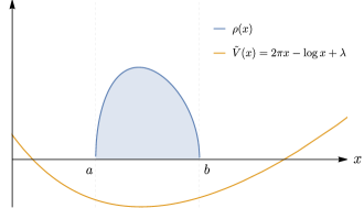
Figure 5: Plot of the density $\rho$ and shifted potential $\tilde{V}(x)=2\pi x-\log{x}+\lambda$ at low density $\beta\equiv 0.015$.

3.1.2 Spin-chain mapping

Equation (97) describes a well-known two-cut matrix-model problem, which appears in various contexts and can be solved exactly (see e.g. refs. DiFrancesco:1993cyw ; muskhelishvili2008singular ; majumdar2009index ; majumdar2011many ; grabsch2017truncated ; tricomi1985integral for reviews of general methods). In particular, it was found to control the classical limit of the XXX_-1/2 Heisenberg spin chain Beisert:2003ea ; Beisert:2003xu . In this case, one considers a collection of $S$ magnons propagating on a closed spin chain of length $J$. The magnons’ momenta are parametrized by a set of roots $\{u_{j},j=1,\ldots,S\}$, quantized by the Bethe ansatz equations

$$\left(\frac{u_{i}+\mathbf{i}/2}{u_{i}-\mathbf{i}/2}\right)^{J}\prod_{j\neq i}^{S}\frac{u_{i}-u_{j}+\mathbf{i}}{u_{i}-u_{j}-\mathbf{i}}=1\,,\qquad i=1,\ldots,S\,.$$ (98)

The classical limit corresponds to $J,S\rightarrow\infty$ while keeping the density $S/J$ fixed. In this limit, the roots scale as $u_{i}=\mathcal{O}(J)$ and the logarithms of the Bethe ansatz equations simplify (see (Beisert:2003ea, , Appendix C)),

$$\frac{J}{u_{i}}+\sum_{j\neq i}^{S}\frac{2}{u_{i}-u_{j}}=2\pi n_{i}\,,$$ (99)

with the so-called mode numbers $n_{i}\in\mathbb{Z}_{\neq 0}$ parametrizing the branches of the logarithms. The ground state corresponds to a symmetric solution, $\{u_{j}\}=\{-u_{j}\}$, with the minimal choice, $n_{j}={\rm sign}{\,u_{j}}$. At large $S$ the roots condense on a symmetric support $\mathcal{C}^{\prime}=(-b,-a)\cup(a,b)$ and the Bethe equations (99) readily reduce to eq. (97) when written in terms of the root distribution density

$$\rho(x)=\frac{1}{J}\sum_{j=1}^{S}\delta(x-u_{j}/J)\,.$$ (100)

One also verifies that the normalizations agree if $\beta=S/J$.

Thanks to this identification, one may read off the solution to our problem from the solution given in refs. Beisert:2003ea ; Beisert:2003xu . It is expressed in terms of elliptic integrals. In particular, the parameters $a,b$ and $\beta$ are given parametrically as

$$a=\frac{1}{4K(q)},\qquad b=\frac{1}{4\sqrt{1-q}K(q)},\qquad\beta=\frac{E(q)}{2\sqrt{1-q}K(q)}-\frac{1}{2}\,,$$ (101)

with $K(q)$ and $E(q)$ the complete elliptic integrals of the 1st and 2nd kind, respectively,

$$K(q)=\int\limits_{0}^{\pi/2}\frac{d\phi}{\sqrt{1-q\sin^{2}{\phi}}}\,,\qquad E(q)=\int\limits_{0}^{\pi/2}d\phi\sqrt{1-q\sin^{2}{\phi}}\,.$$ (102)

Here, $q\in(0,1)$ with the lower/upper bound corresponding respectively to $\beta\rightarrow 0$ and $\beta\rightarrow\infty$. One may also express the density $\rho(x)$ in closed form, in terms of the incomplete elliptic integral of the third kind. (See eqs. (C.7) and (C.8) in appendix C of ref. Beisert:2003ea .) We plot $\rho(x)$ in figure 5 for illustration. We will not need its explicit analytic expression here, but it will be useful to know its derivative with respect to $\beta$, $\delta\rho=\partial_{\beta}\rho$.

The derivative of the density is rather simple to construct. Differentiating both sides of eq. (95) with respect to $\beta$, the potential drops out. Using also the vanishing of $\rho$ at the boundaries, $\rho(a)=\rho(b)=0$, one is left with a simpler (homogeneous) problem

$$\partial_{\beta}\lambda=2\int\limits_{a}^{b}\mathrm{d}y\delta\rho(y)\log{|x^{2}-y^{2}|}\,,\qquad\forall x\in(a,b)\,.$$ (103)

In the Coulomb gas picture, this equation describes a collection of charges with no external potential, but subject to hard-wall boundary conditions at $a$ and $b$. So, despite the absence of a potential, the charges do not run away but accumulate close to the boundaries, $c=a,b$, where $\delta\rho(x)\sim 1/\sqrt{|x-c|}$.

Taking a derivative of eq. (103) with respect to $x$ removes the left-hand side of the equation, and the solution is immediately obtained using a standard inversion formula,

$$\delta\rho=\frac{x}{\pi\sqrt{(b^{2}-x^{2})(x^{2}-a^{2})}}\,.$$ (104)

The only freedom here is the overall normalization, which is fixed using

$$\delta\int\limits_{a}^{b}\mathrm{d}x\rho(x)=\int\limits_{a}^{b}\mathrm{d}x\,\delta\rho(x)=\frac{\partial}{\partial\beta}\frac{\beta}{2}=\frac{1}{2}\,,$$ (105)

taking into account again that the boundary terms vanish.

3.1.3 Differential equation I

The next step is to calculate the scaling function (93). This may be done in principle using the exact solution for $\rho$ given in refs. Beisert:2003ea ; Beisert:2003xu . Its direct integration proves difficult however. So, here we shall consider the much simpler problem of determining $df/d\beta$ using the density derivative $\delta\rho=\partial_{\beta}\rho$.

Observe first that eq. (93) simplifies when evaluated on the saddle point. Acting with $\int\mathrm{d}x\rho(x)$ on both sides of eq. (95) and using the normalisation condition (88), one finds the relation

$$\tfrac{1}{2}\beta\lambda=\int_{a}^{b}\mathrm{d}x\rho(x)(\log{x}-2\pi x)+2\int_{a}^{b}\int_{a}^{b}\mathrm{d}x\mathrm{d}y\rho(x)\rho(y)\log{|x^{2}-y^{2}|}\,,$$ (106)

which may be used to eliminate the double integral in eq. (93),

$$\beta^{2}(f-f_{0})=\beta\lambda+2\int_{a}^{b}\mathrm{d}x\rho(x)(\log{x}-2\pi x)\,,$$ (107)

with $f_{0}$ given in eq. (94). A derivative with respect to $\beta$ then yields

$$\frac{d}{d\beta}(\beta^{2}(f-f_{0}))=\lambda+\beta\partial_{\beta}\lambda+2\int_{a}^{b}\mathrm{d}x\,\delta\rho(x)(\log{x}-2\pi x)\,,$$ (108)

using that $\delta\int=\int\delta$ since $\rho$ vanishes at the boundary.

One may further simplify the right-hand side of eq. (108), by acting on eq. (95) and eq. (103) with $2\int\mathrm{d}x\delta\rho(x)$ and $2\int\mathrm{d}x\rho(x)$, respectively, and taking their difference,

$$\lambda=\beta\partial_{\beta}\lambda+2\int_{a}^{b}\mathrm{d}x\,\delta\rho(x)(\log{x}-2\pi x)\qquad\Rightarrow\qquad\frac{d}{d\beta}(\beta^{2}(f-f_{0}))=2\lambda\,.$$ (109)

The integral on the right-hand side of the equation for $\lambda$, as well as the one defining $\partial_{\beta}\lambda$, see eq. (103), can be taken immediately using eq. (104),

$$\partial_{\beta}\lambda=\log{\left[\frac{b^{2}-a^{2}}{4}\right]}\,,\qquad\int_{a}^{b}\mathrm{d}x\,\delta\rho(x)(\log{x}-2\pi x)=\frac{1}{2}\log{\left[\frac{a+b}{2}\right]}-\beta-\frac{1}{2}\,.$$ (110)

Finally, eliminating $\lambda$ yields

$$\frac{d}{d\beta}\Big{[}\beta^{2}(f-f_{0})\Big{]}=2\beta\log{\left[\frac{b^{2}-a^{2}}{4}\right]}+2\log{\left[\frac{a+b}{2}\right]}-4\beta-2\,,$$ (111)

with $a,b,\beta$ related to each other through eq. (101).

This first-order differential equation determines $f$ uniquely, once supplemented with the boundary condition $\lim_{\beta\rightarrow 0}(\beta^{2}f)=0$. The boundary condition follows from (107), using that $b\rightarrow a$ when $\beta\rightarrow 0$, and $\lim_{\beta\rightarrow 0}(\beta^{2}f_{0})=0$ from eq. (94).

The differential equation (111) can be integrated directly around particular points, such as $\beta=0$ or $\infty$, after evaluating its right-hand side using eqs. (101). It is less straightforward to integrate it for general $\beta$, given the complicated dependence of the coefficients $a,b$ on $\beta$. Fortunately, we will not need to deal with this problem here, as the solution will come for free after combining eq. (111) with a similar equation controlling the thermodynamic limit of the BMN integral.

3.2 BMN integral

Consider now the BMN integral (26). In this case, instead of a single matrix-model integral, we have an ensemble of integrals, labelled by integers $\{a_{\ell}\}$. However, at large $m$, we expect it to be dominated by the lowest modes, with $a_{\ell}=1,\forall\ell=1,\ldots,m$. This is because the external potential

$$V_{a}(u)=(m+n)\log{(u^{2}+a^{2}/4)}$$ (112)

has its minimum at $a=1$ and generates power suppressions for the higher $a$’s in the thermodynamic limit. Owing to this truncation, there is no dependence on $\varphi$, and similarly $\sigma$ drops out, for $\sigma,\varphi=\mathcal{O}(1)$. In summary, focusing on the leading saddle, one may write

$$\Phi_{m,n}\approx\frac{d(z,\bar{z})^{m}}{(2\pi)^{m}m!}\times\int_{\mathbb{R}^{m}}\prod_{\ell=1}^{m}\frac{\mathrm{d}u_{\ell}}{(u_{\ell}^{2}+1/4)^{m+n}}\prod_{i<j}^{m}\left[(u_{i}-u_{j})^{2}((u_{i}-u_{j})^{2}+1)\right]\,.$$ (113)

Furthermore, one notes that the potential (112) scales linearly with $m$, for all $u$’s. Hence, there is no need to rescale the rapidities here and we can proceed directly to the thermodynamic limit with the density

$$\rho(u)=\frac{1}{m}\sum_{i=1}^{m}\delta(u-u_{i})\,,$$ (114)

which we expect to be smooth for $u=\mathcal{O}(m^{0})$. Varying the integral (113), we get

$$0=\frac{(k+1)u}{u^{2}+1/4}-\mathchoice{{\vbox{\hbox{$\textstyle-$}}\kern-4.86108pt}}{{\vbox{\hbox{$\scriptstyle-$}}\kern-3.25pt}}{{\vbox{\hbox{$\scriptscriptstyle-$}}\kern-2.29166pt}}{{\vbox{\hbox{$\scriptscriptstyle-$}}\kern-1.875pt}}\!\int_{-B}^{B}\mathrm{d}v\rho(v)\Big{[}\frac{u-v}{(u-v)^{2}+1}+\frac{1}{u-v}\Big{]}\,,\qquad\forall u\in(-B,B)\,,$$ (115)

assuming that the density is even and supported on a compact interval $(-B,B)$, as suggested by the symmetry and convexity of the potential. We seek a solution obeying the usual boundary conditions

$$\rho(u)\propto\sqrt{B^{2}-u^{2}}\,,\qquad u\sim\pm B\,,$$ (116)

and normalized such that

$$\int_{-B}^{B}\mathrm{d}v\,\rho(v)=1\,.$$ (117)

3.2.1 Resolvent

Equation (115) can be solved immediately in the two extreme regimes, $k\rightarrow\infty$ and $k\rightarrow 1$. The former corresponds to a dilute gas approximation, $B\rightarrow 0$, where the singular part $\sim 1/(u-v)$ of the kernel dominates and the potential becomes linear. Thus it reduces to the Gaussian matrix model and the associated semi-circle law

$$\rho(u)\approx\frac{2}{\pi B^{2}}\sqrt{B^{2}-u^{2}}\,,$$ (118)

with $B\sim 1/\sqrt{2k}$. The opposite limit, $B\rightarrow\infty$, maps to $k\rightarrow 1$, and the equation may be solved by a Fourier transform over the entire real axis,

$$\lim_{k\rightarrow 1}\rho(u)=\operatorname{sech}{(\pi u)}\,.$$ (119)

The problem gets harder in the intermediate regime $k\in(1,\infty)$. It can nonetheless be solved exactly by following a method introduced in ref. Kazakov:1998ji to tackle a similar looking matrix-model equation.

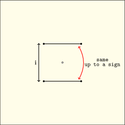
Figure 6: Riemann sheet structure of the resolvent $r(u)$. There is a simple pole at the origin (and at infinity) and two cuts of length $2B$ spaced by $\mathbf{i}$. The periodicity condition identifies the values of the functions above and below the cuts, up to a sign.

To begin, we define the function

$$r(u)=\frac{k+1}{u}-\int\limits_{-B}^{B}\mathrm{d}v\frac{2(u-v)\rho(v)}{(u-v)^{2}+1/4}\,.$$ (120)

It is analytic in $\mathbb{C}$, except along the intervals $(-B\pm\mathbf{i}/2,+B\pm\mathbf{i}/2)$, where it has square-root branch cuts, and at $u=0$, where it has a simple pole, $r(u)\sim(k+1)/u$. We also note that the function has a pole at $u=\infty$, with residue

$$\lim_{u\rightarrow\infty}u\,r(u)=k+1-2\int\limits_{-B}^{B}\mathrm{d}v\rho(v)=k-1\,.$$ (121)

The function $r$ relates to the standard (single-cut) resolvent

$$R(u)=\int\limits_{-B}^{B}\frac{\mathrm{d}v\rho(v)}{u-v}\qquad\Rightarrow\qquad r(u)=\frac{k+1}{u}-(R(u+\mathbf{i}/2)+R(u-\mathbf{i}/2))\,,$$ (122)

implying that one may recover the density $\rho(u)$ from the discontinuities of $r(u)$ across either cut,

$$\rho(u)=\frac{1}{2\pi\mathbf{i}}\Bigl{[}r(u\pm\mathbf{i}/2+\mathbf{i}0)-r(u\pm\mathbf{i}/2-\mathbf{i}0)\Bigr{]}\,,\qquad\forall u\in(-B,B)\,.$$ (123)

In particular, it follows from this relation that $r(u)$ must be continuous at the branch points $u=\pm\mathbf{i}/2\pm B$, since the density vanishes at $u=\pm B$, see eq. (116).

The main motivation for introducing a resolvent in this way is that the saddle-point equation (115) now takes the simple form

$$r(u+\mathbf{i}/2-\mathbf{i}0)+r(u-\mathbf{i}/2+\mathbf{i}0)=0,\qquad\forall u\in(-B,B)\,.$$ (124)

It implies that $r(u)$ extends to an anti-periodic function of period $\mathbf{i}$ on the second Riemann sheet, that is, after continuing below the cuts, see figure 6.

In addition, the resolvent $r$ possesses important reality and reflection properties,

$$r(u)=(r(u^{*}))^{*}\,,\qquad r(u)=-r(-u)\,,$$ (125)

with $*$ denoting complex conjugation, which stem from the fact that $\rho$ is a real symmetric function. It then suffices to find $r$ on the first quadrant, in order to determine it everywhere else. Taking the cuts into account, we should in fact consider the open domain $D$ shown in the left panel of figure 7, which is obtained by removing the segment between $u=\mathbf{i}/2$ and $u=B+\mathbf{i}/2$ from the first quadrant.

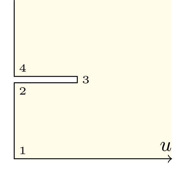
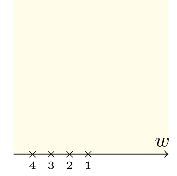
$\xlongleftrightarrow{\textrm{SC}}$    $u$   $w$    $u_{1}=0$  $w_{1}=0$    $u_{2}=\frac{\mathbf{i}}{2}-\mathbf{i}0$   $w_{2}$    $u_{3}=\frac{\mathbf{i}}{2}+B$   $w_{3}$    $u_{4}=\frac{\mathbf{i}}{2}+\mathbf{i}0$   $w_{4}$    $\infty$ $\infty$

Figure 7: The conformal mapping $u\rightarrow w=1/r(u)^{2}$ maps the domain $D$ to the upper half-plane $\mathbb{H}$, and vice versa. In particular, the boundaries map into each other owing to the reflection symmetry and periodicity of $r(u)$. The table indicates the values of the map at the marked points on the boundary.

3.2.2 Schwarz-Christoffel mapping

The function $r$ obeys simple functional relations, but is defined over a complicated domain. The next step is to make the domain more regular with the help of a Schwarz-Christoffel (SC) transformation. Namely, $D$ can be seen as the interior of a polygon (with a vertex at infinity) and as such can be mapped conformally to the upper half-plane $\mathbb{H}=\{w\in\mathbb{C}:\textrm{Im}\,w>0\}$ with the boundary $\partial D$ mapping to the real $w$ axis. The map is constructed canonically, using the interior angles at the vertices of $\partial D$ to determine the exponents in the SC transform $w\rightarrow u$. Fixing $u=w=0$ and $u=w=\infty$ for simplicity, we get

$$u=A\int_{0}^{w}\frac{(t-w_{3})\mathrm{d}t}{\sqrt{t(t-w_{2})(t-w_{4})}}\,,$$ (126)

with $w_{4}<w_{3}<w_{2}<0$ the images of $u_{4}=\mathbf{i}/2+\mathbf{i}0\,,u_{3}=\mathbf{i}/2+B$ and $u_{2}=\mathbf{i}/2-\mathbf{i}0$, respectively, and with $A>0$ an arbitrary normalization factor, introduced for later convenience.

We may now easily express the resolvent $r$ as a function of $w$. The key observation is that the map

$$\mathcal{F}:w\rightarrow\mathcal{F}(w)=1/r(u(w))^{2}$$ (127)

is a holomorphic bijective function of $\mathbb{H}$ to itself, that is, a real Möbius transformation. This is manifest in the neighbourhood of $w=0$ or $w=\infty$. At these points, $r(u)\sim(k\pm 1)/u$ and $\sqrt{w}/u$ is constant. Hence, one can always write

$$r(u)=\frac{1}{\sqrt{w}}\,,$$ (128)

for a suitable choice of the parameters $A,w_{2,3,4}$, see eq. (130) below. The claim is that eq. (128) holds globally, for all $w\in\mathbb{H}$.

To justify the claim, it is enough to show that $\mathcal{F}$ extends to a continuous function of the closed upper half-plane taking real values on the real axis. The Schwarz reflection principle can then be used to conclude that $\mathcal{F}$ extends to an entire function on $\mathbb{C}$ and thus $\mathcal{F}(w)=w$ given the asymptotic behaviours at $0$ and $\infty$.

Now, it is easy to show that $\mathcal{F}$ preserves the boundary $\partial\mathbb{H}$. This follows directly from the reality and periodicity properties of $r$. Namely, $r(u)$ is respectively real for $u\in(0,\infty)$ and purely imaginary for $u\in(0,\mathbf{i}\infty)$, because of eq. (125). It is also purely imaginary just below the cut, i.e. $u\in(u_{2},u_{3})$, owing to eq. (124),

$$r(u+\mathbf{i}/2-\mathbf{i}0)^{*}=r(u-\mathbf{i}/2+\mathbf{i}0)=-r(u+\mathbf{i}/2-\mathbf{i}0)\,,$$ (129)

and similarly for $u\in(u_{3},u_{4})$, thanks to the discontinuity formula (124) and the reality of $\rho$. Furthermore, $\mathcal{F}$ is continuous on $\partial\mathbb{H}$, including at the fold-point $w=w_{3}$, since $\rho(u)$ vanishes at $u=u_{3}$, and at the origin $w=0$, where $\mathcal{F}\rightarrow 0$. Hence, as desired, $\mathcal{F}$ maps $\partial\mathbb{H}$ into itself.

Finally, one may determine the unfixed parameters $(A,w_{2,3,4})$ in the SC transformation, by matching both sides of eq. (128) at the marked points on the boundary. The analysis is deferred to appendix B. The results can be written concisely in terms of the elliptic data $a,b,q$ introduced in eqs. (101),

$$A=\frac{1}{2\beta}\,,\qquad w_{2}=\frac{-\beta^{2}}{16\pi^{2}b^{2}}\,,\qquad w_{3}=\frac{-\beta^{2}(1+2\beta)}{16\pi^{2}ab}\,,\qquad w_{4}=\frac{-\beta^{2}}{16\pi^{2}a^{2}}\,,$$ (130)

with $\beta=1/(k-1)$ and with the modulus $q=1-w_{2}/w_{4}\in(0,1)$.

3.2.3 Duality map

Prior to moving on to the calculation of the free energy, let us open a parenthesis here to comment on the relation between the above solution and the one constructed earlier. The two solutions should be images of each other, as they are based on two equivalent representations, for any $m$ and $n$. In practice, however, it is not easy to follow the Mellin-Barnes transformation used in section 2.2 all the way to the large $m$ limit. One may nonetheless find the duality map directly in this limit from a comparison of the two saddle-point solutions.

Recall first of all that the interval $(a,b)$ determines the support of the dual density, denoted $\rho_{\textrm{dual}}(x)$ here, to avoid confusion. Looking at (130), we see that this interval can be identified with the segment $(w_{2},w_{3})$ of the $w$ plane. More precisely, the above relations suggest to set

$$x=\frac{\mathbf{i}\beta}{4\pi\sqrt{w}}=\frac{\mathbf{i}\beta r(u)}{4\pi}\,,$$ (131)

thus identifying the image of the resolvent $r(u)$ with the dual $x$ plane. The reciprocal relation identifies the $u$ plane with the image of a suitable resolvent $r_{\textrm{dual}}(x)$ for the dual problem,

$$u=\frac{\mathbf{i}}{2\pi}r_{\textrm{dual}}(x)\,.$$ (132)

This relation can be worked out from the elliptic parametrization (126) together with (131). One may also proceed as follows. Using the map (131) and properties of $r(u)$, one easily sees that the inverse map $r_{\textrm{dual}}(x)=-r_{\textrm{dual}}(-x)$ is an analytic function of $x$ with square-root cuts along $(-b,-a)\cup(a,b)$ and poles at $x=0$ and $x=\infty$, with residues

$$r_{\textrm{dual}}(x)\sim\frac{1}{2x}\,,\qquad r_{\textrm{dual}}(x)\sim\frac{k+1}{2(k-1)x}\,,$$ (133)

respectively. It must also obey the equation

$$r_{\textrm{dual}}(x+\mathbf{i}0)+r_{\textrm{dual}}(x-\mathbf{i}0)=2\pi\mathbf{i}(u^{*}-u)=2\pi\,,$$ (134)

for any $x\in(a,b)$, since on this interval $\textrm{Im}\,u=\mathbf{i}/2$ according to eq. (131), see table in figure 7. These requirements define a Riemann-Hilbert problem whose solution is given by

$$r_{\textrm{dual}}(x)=\frac{1}{2x}+\int\limits_{a}^{b}\frac{2x\rho_{\textrm{dual}}(y)\mathrm{d}y}{x^{2}-y^{2}}\,,$$ (135)

for $x\notin(a,b)$, with $\rho_{\textrm{dual}}(x)$ the density constructed in the previous section. In particular, equations (133) and (134) are easily checked using (88) and the dual saddle-point equation (96). At last, $r_{\textrm{dual}}(x)$ is seen to be a resolvent for the dual problem, since

$$\rho_{\textrm{dual}}(x)=\frac{\mathbf{i}}{2\pi}(r_{\textrm{dual}}(x+\mathbf{i}0)-r_{\textrm{dual}}(x-\mathbf{i}0))=\textrm{Re}\,u\,,$$ (136)

for any $x\in(a,b)$. Hence, nicely, the large $m$ duality map merely interchanges rapidities and resolvents of the two problems.

3.2.4 Differential equation II

We may now calculate $df/dk$ using the density of the BMN integral (113). The starting point is the saddle-point expression obtained from eq. (113),

$$f(k)=-(1+k)\int\mathrm{d}u\rho(u)\log(u^{2}+\tfrac{1}{4})+\frac{1}{2}\int\mathrm{d}u\mathrm{d}v\rho(u)\rho(v)\log[(u-v)^{2}((u-v)^{2}+\tfrac{1}{4})]\,,$$ (137)

which is extremal on the just-constructed solution $\rho$,

$$\mu=\frac{\delta f}{\delta\rho(u)}=-(1+k)\log(u^{2}+\tfrac{1}{4})+\int\mathrm{d}v\rho(v)\log[(u-v)^{2}((u-v)^{2}+\tfrac{1}{4})]\,,$$ (138)

with $\mu$ a Lagrange multiplier for $\int\rho(u)\mathrm{d}u=1$. These relations imply that

$$\frac{\mathrm{d}f}{\mathrm{d}k} =-\int\mathrm{d}u[\rho(u)+(k+1)\delta\rho(u)]\log(u^{2}+\tfrac{1}{4})+\int\mathrm{d}u\mathrm{d}v\delta\rho(u)\rho(v)\log[(u-v)^{2}((u-v)^{2}+\tfrac{1}{4})]$$ (139)

$$=-\int\mathrm{d}u\rho(u)\log(u^{2}+\tfrac{1}{4})+\mu\int\mathrm{d}u\,\delta\rho(u)=-\int\mathrm{d}u\rho(u)\log(u^{2}+\tfrac{1}{4})\,,$$

with $\delta\rho=d\rho/dk$, after eliminating the double integration with eq. (138) and using $\delta\int\rho=\int\delta\rho=0$.

We then introduce an auxiliary function,

$$h(u)=\int_{-B}^{B}\mathrm{d}v\rho(v)\log[(u-v)^{2}+\tfrac{1}{4}]\,,$$ (140)

which returns $-df/dk$ when evaluated at $u=0$. This function is nothing but an integrated version of the resolvent $r(u)$, with given large $u$ behavior,

$$\frac{\mathrm{d}h(u)}{\mathrm{d}u} =\frac{k+1}{u}-r(u)\,,\qquad h(u)=2\log{u}+\mathcal{O}(1/u^{2})\,.$$ (141)

This equation can be integrated with the help of eqs. (126) and (128). It yields

$$h(u) =(k+1)\log{u}-(k-1)\int^{w}\frac{\mathrm{d}t}{2t}\frac{t-w_{3}}{\sqrt{(t-w_{2})(t-w_{4})}}$$ (142)

$$=(k+1)\log{u}-(k-1)\log{(\sqrt{w-w_{4}}+\sqrt{w-w_{2}})}+(k+1)\,{\rm arctanh}{\,\sqrt{\frac{(w-w_{4})w_{2}}{(w-w_{2})w_{4}}}}+cte\,,$$

up to a constant of integration, fixed by the large $u$ asymptotics,

$$cte=-(k-1)\log\Big{[}\tfrac{1}{2}(k-1)\Big{]}-(k+1)\log{\sqrt{\frac{b+a}{b-a}}}\,,$$ (143)

using $u\sim(k-1)\sqrt{w}\gg 1$ and eq. (130). Lastly, the limit $u\rightarrow 0$ yields

$$\frac{\mathrm{d}f}{\mathrm{d}k}=2k\log\Big{[}\tfrac{1}{2}(a+b)\Big{]}-(k-1)\log{(ab)}+2\log{(4\pi)}+(k+1)\log{\left[\frac{k-1}{k+1}\right]}\,,$$ (144)

using $u\sim(1+k)\sqrt{w}\ll 1$ (see appendix B) and switching to variables $a,b$ with eq. (130).

3.3 Free energy

We shall now derive a parametric representation for the scaling function $F(k)=f(k)/k$. From eq. (92) we see that $F(k)$ is normalized by the rectangle area $mn$ rather than $m^{2}$.

3.3.1 Parametric representation

A key simplification arises when combining our two differential equations, eqs. (111) and (144). Namely, one finds that the function $f$ can be extracted directly, without any integration. This is possible because the equations are linearly independent and have only one solution in common. Taking the sum of the two equations eliminates the derivatives of $f$,

$$\frac{d}{d\beta}(\beta^{2}(f-f_{0}))+\frac{d}{dk}f=2\beta f-\frac{d}{d\beta}(\beta^{2}f_{0})\,,$$ (145)

giving

$$f=\log\Big{[}\tfrac{1}{2}(b-a)\Big{]}+k^{2}\log\Big{[}\tfrac{1}{2}(a+b)\Big{]}-\frac{(k-1)^{2}}{2}\log{(ab)}+2k\log{(4\pi)}+\frac{(k+1)^{2}}{2}\log{\left[\frac{k-1}{k+1}\right]}\,,$$ (147)

after using eqs. (111), (144), (94) and $\beta=1/(k-1)$.

As a double check, one may verify that this expression solves each differential equation separately. For this purpose, it is useful to have the $\beta$ derivatives of $a$ and $b$,

$$\frac{da}{d\beta}=\frac{2a^{2}}{2a\beta+a-b}\,,\qquad\frac{db}{d\beta}=\frac{2b^{2}}{2b\beta+b-a}\,,$$ (148)

which follow from eq. (101) and the chain rule.

Introducing $F(k)=f(k)/k$ and using eq. (101), one arrives at

$$\begin{aligned} F(k)=\log{\pi^{2}}&+k\log\Big{(}\frac{1+\sqrt{1-q}}{2}\Big{)}+\frac{(k-1)^{2}}{2k}\log{K(q)}\\ &+\frac{1}{k}\log\Big{(}\frac{1-\sqrt{1-q}}{2}\Big{)}-\frac{(k+1)^{2}}{2k}\log{E(q)}\,,\\ \end{aligned}\$$ (149)

where we recall that

$$k=\frac{E(q)+\sqrt{1-q}K(q)}{E(q)-\sqrt{1-q}K(q)}\,,$$ (150)

with $K(q)$ and $E(q)$ the complete elliptic integrals, see eq. (102), and $q\in(0,1)$.

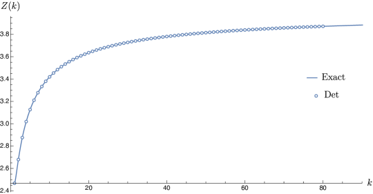
Figure 8: Plot of $Z(k)=e^{F(k)}$ for $k\in[1,90]$. The data points are obtained by extrapolating numerically the determinant at large $m,n$ for $z=\bar{z}=-1$ and $k\in\{1,80\}$. The solid line is obtained using the parametric representation, eqs. (149) and (150). $Z(k)$ is seen to be monotonic and bounded by $Z(1)=\pi^{2}/4=2.4674...$ and $Z(\infty)=4$.

The system of equations (149) and (150) is our final expression for the free-energy density. It determines $F(k)$ parametrically over the whole domain $k\in(1,\infty)$. Figure 8 shows the comparison between this scaling function and a numerical estimate of the ladder determinant (6) for large $m$ and $n$. As one can see, the agreement is excellent for all accessible values of $k$.

Note that one may first simplify the determinant to facilitate the comparison. Since the cross ratios drop out in this regime, one can conveniently set $\varphi=\sigma=0$, or equivalently send $z,\bar{z}\rightarrow-1$, in eq. (5), giving

$$\Phi_{m,n}\approx\frac{1}{\mathcal{N}}\det\,(a_{i+j+n-m-1})_{1\leqslant i,j\leqslant m}\,,$$ (151)

with $a_{p}=8(1-4^{1-p})(2p-1)!\zeta(2p-1)$, using $L_{p}(z,\bar{z})\approx 2(z-\bar{z})(1-4^{1-p}){{2p-1}\choose{p-1}}\zeta(2p-1)$.

Below, we study in detail the behaviour of the free energy at $k=\infty$ and $k=1$, using known asymptotic expressions for the elliptic integrals at $q=0$ and $q=1$. These points are of particular interest since they correspond to the ladder limit $n\gg m$ and to the symmetric point $n=m$, respectively.

3.3.2 Ladder limit

The limit $k\rightarrow\infty$ corresponds to $q\rightarrow 0^{+}$. The elliptic integrals are regular at this point and admit convergent expansions in integer powers of $q$,

$$K(q)=\frac{\pi}{2}+\frac{\pi q}{8}+\mathcal{O}(q^{2}),\qquad E(q)=\frac{\pi}{2}-\frac{\pi q}{8}+\mathcal{O}(q^{2})\,,$$ (152)

from which it follows that

$$q=\frac{4\sqrt{2}}{\sqrt{k}}-\frac{16}{k}+\mathcal{O}(\frac{1}{k^{3/2}})\,,$$ (153)

using eq. (150). Expanding further and plugging the series inside eq. (149), one finds

$$F(k)=\log{4}-\frac{2\log{\left(\frac{k}{2}\right)}+3}{4k}-\frac{1}{8k^{2}}+\frac{19}{384k^{3}}-\frac{7}{512k^{4}}+\frac{301}{30720k^{5}}-\frac{81}{20480k^{6}}+\mathcal{O}\Big{(}\frac{1}{k^{7}}\Big{)}\,.$$ (154)

Notice that the half-integer powers of $1/k$ in the expansion of $q$ cancel out in $F$. Hence, $F$ admits a regular expansion in $1/k$, up to a logarithm $\sim\log{k}/k$. The series is seen to alternate and it approximates the exact curve extremely well throughout the entire domain, including the point $k=1$, where (154) is found to converge rather quickly towards the exact value $F(1)=\log{(\pi^{2}/4)}$. It suggests that the series converges for all $k\in[1,\infty)$.

The leading term in this expansion has a simple interpretation. As seen earlier, the limit $k\rightarrow\infty$ corresponds to a dilute gas approximation, which means that the free energy is a multiple of the free energy of an individual ladder $L_{p}$ at large $p$. This is easily verified using the definition (9). At large weight, the polylogarithm series (9) truncates,

$$\textrm{Li}_{j}(z)\approx z\,,$$ (155)

assuming $|z|<1$ for convenience, and the sum $\sum_{j=p}^{2p}$ in eq. (9) is dominated by the terms with $j\sim 2p$. One can thus take the large $p$ limit of the summand at fixed $l=2p-j$, using Stirling’s approximation for the factorials, and perform the sum over $l=0,1,\ldots\,$,

$$L_{p}(z,\bar{z})\approx(z-\bar{z})\sum_{l=0}^{p}\frac{(2p-l)!}{p!\,l!\,(p-l)!}[-\log{(z\bar{z})}]^{l}\approx\frac{4^{p}(z-\bar{z})}{\sqrt{\pi pz\bar{z}}}\,.$$ (156)

It yields $\lim_{p\rightarrow\infty}\frac{1}{p}\log{\left[L_{p}(z,\bar{z})\right]}=\log{4}=1.386...\,,$ in agreement with $F(\infty)$.

3.3.3 Square limit

The limit $k\rightarrow 1$ corresponds to $q\rightarrow 1^{-}$ and in this limit

$$\lim\limits_{k\rightarrow 1}F(k)=\log{(\pi^{2}/4)}=0.903...\,.$$ (157)

Subleading corrections have a complicated pattern, involving not only powers of $(k-1)$ but also of its logarithms. This feature goes back to logarithms in the expansion of the elliptic integrals around $q=1$,

$$K(q)=-\frac{1}{\pi}K(1-q)\log{(1-q)}+\ldots\,,$$ (158)

$$E(q)=-\frac{1}{\pi}(K(1-q)-E(1-q))\log{(1-q)}+\ldots\,,$$

with the dots standing for regular series in $(1-q)$.

A double expansion is easily generated as follows. First, define the variable

$$\zeta=\frac{k-1}{\sqrt{k}}=\frac{2\sqrt{1-q}\,K(q)}{\sqrt{E(q)^{2}-(1-q)K(q)^{2}}}\,,$$ (159)

which is small when $k\rightarrow 1$ and changes sign under $k\rightarrow 1/k$, and then introduce the ansatz

$$q=1-16\zeta^{2}\bigg{[}\alpha^{2}(\log\zeta)+\sum_{n=1}^{\infty}\zeta^{n}\alpha_{n}(\log\zeta)\bigg{]}\,,$$ (160)

with the expansion coefficients, $\alpha$ and $\alpha_{n}$, being functions of $\log{\zeta}$. The latter coefficients are determined self-consistently, by plugging (160) inside eq. (159), expanding in powers of $\zeta$ and matching the coefficients on both sides of the equation. For instance, at the leading order in $\zeta$, one finds

$$\zeta=-8\zeta\alpha\log{(\zeta\alpha)}+\mathcal{O}(\zeta^{2})\,,$$ (161)

or equivalently

$$\alpha=-\frac{1}{8\log{\zeta}}\left[1+\frac{\log{(-8\log{\zeta})}}{\log{\zeta}}+\mathcal{O}\left(\frac{\log^{2}{(-\log{\zeta})}}{\log^{2}{\zeta}}\right)\right]\,.$$ (162)

The full solution for $\alpha=\alpha(\log{\zeta})$ can also be given in closed form,

$$\alpha=-\frac{1}{8W_{-1}(-\frac{\zeta}{8})}\,,$$ (163)

with $W_{-1}(x)$ the second branch of the Lambert $W$ function, defined for $x\in(-1/e,0)$ and such that

$$W_{-1}(x)=\log{(-x)}-\log{(-\log{(-x)})}+\ldots\,,$$ (164)

when $x\rightarrow 0^{-}$.

Cancelling the terms at higher orders in eq. (161) determines the higher coefficients $\alpha_{n}$ recursively. One finds that $\alpha_{n}=0$ when $n$ is odd, in line with the $k\leftrightarrow 1/k$ (dihedral) symmetry of the correlator, and one observes that the non-vanishing coefficients can be expressed in terms of $\alpha$. The first few terms read

$$F(k)=\log{\left[\frac{\pi^{2}}{4}\right]}+[2(3-4\alpha)\alpha-\frac{1}{2}\log(32\alpha)]\zeta^{2}+\frac{\alpha}{6}[3-2\alpha(9+4\alpha(-5+6\alpha))]\zeta^{4}+\mathcal{O}(\zeta^{6})\,,$$ (165)

which is thus an even regular series, up to the tails of logarithms encoded in eq. (162). We remark that the expansion (165) has a very small range of validity if $\alpha$ is given by eq. (162).

3.4 Comparison with periodic fishnets

It is instructive to compare our formula with the large-order behaviour of fishnet graphs with doubly periodic boundary conditions. In his pioneering paper, A. Zamolodchikov Zamolodchikov:1980mb obtained the expression for the $m\times n$ fishnet torus partition function $Z_{m,n}$, in any spacetime dimensions $D$, using integrability and bootstrap conditions. Assuming the thermodynamic scaling, he found that

$$\lim_{m,n\rightarrow\infty}\frac{1}{mn}\log{Z_{m,n}}=-\log{g_{c}^{2}}\,,$$ (166)

where the so-called critical coupling $g_{c}$ is a constant which depends on $D$ but not on the fishnet lengths $m,n$. The explicit expression for $D=4$ is given by Zamolodchikov:1980mb

$$-\log{g_{c}^{2}}=\log{\left[\frac{\Gamma(\tfrac{1}{4})^{4}}{32\pi}\right]}=0.541...\,.$$ (167)

Clearly, this result bears no similarity at all with our general expression for $F(k)$. It is also numerically different, over the whole physical range $k\in(1,\infty)$; it is just over half of the lowest value achieved by $F(k)$, namely $F(1)=\log{(\pi^{2}/4)}=0.903...$.

From the 2d lattice perspective, this discrepancy and, more generally, the dependence of the scaling function $F$ on the aspect ratio $k$ appear surprising at first sight. They go against the common wisdom that the thermodynamic free energy is extensive and independent of the boundary conditions. Put differently, they suggest that the boundary conditions set by the four-point fishnet correlator are atypical and “severe” enough to penetrate deeply into the bulk of the lattice, in such a way that the uniform periodic distribution may hold only locally, far away from the boundary, if at all.

This sensitivity to the boundary conditions is likely to hold for other correlators. In fact a similar phenomenon may be observed for half-periodic fishnets, mixing open and closed boundary conditions, such as the one shown in the right panel of figure 1. An interesting aspect of these mixed boundary conditions is that they provide a regularization of the otherwise ill-defined doubly periodic fishnets, which suffer from UV/IR divergences. They yield finite correlation functions, which depend on several cross ratios and which may be expanded over a complete basis of states in principal series representations, as discussed in detail in ref. Grabner:2017pgm in a particular case. Doing so, one projects over states carrying arbitrary scaling dimension $\Delta$ along the radial direction.. Fishnets of this type were considered in the thermodynamic limit in ref. Basso:2018agi , for certain states, and their free energy was calculated for a large range of scaling dimensions $\Delta$ using the Thermodynamic Bethe Ansatz (TBA) equations of the fishnet theory. Importantly, they were found to scale as in (166) only for $\Delta$’s that are much smaller than the fishnet size. The latter requirement is understood as a condition for the validity of the continuum description of large fishnet graphs, which is governed in the case at hand by the 2d non-linear $AdS_{5}$ sigma model. If on the contrary the dimension $\Delta$ scales large with the system size, then the corresponding state in the sigma model is very excited, with a finite energy density, and the free energy density departs significantly from the ground-state behavior (166).

Another way of phrasing the situation is in terms of the so-called graph building operator $T_{m}$ Gromov:2017cja ; Zamolodchikov:1980mb , which is the integral kernel which adds a rung to periodic fishnet graphs with $m$ radial lines. It may be interpreted as a finite-time evolution operator for an integrable spin chain, with spins in a suitable representation of the four-dimensional conformal group Gromov:2017cja ; Derkachov:2020zvv . Its logarithm defines a Hamiltonian for a system of length $m$, which is well approximated by the Hamiltonian of the $AdS_{5}$ sigma model,

$$-\log{T_{m}}=m\log{g^{2}_{c}}+H_{AdS}+\ldots\,,$$ (168)

in the large volume limit $m\rightarrow\infty$, up to higher-derivative interactions associated with $1/m$ corrections. The point is that this expansion can be trusted, and the latter corrections neglected, only when the quantum numbers of the state, and in particular the scaling dimension, are much smaller than the length $m$. One may expect this condition to be observed for $m\times n$ half-periodic fishnets, at generic values of the cross ratios, as long as both $m$ and $n$ are large – with the limit of large number of rungs (or large discrete time), $n\rightarrow\infty$, being used here to project on the 2d low-energy states. However, it is not obeyed, even for large $m$ and large $n$, for the special configurations of the boundary points which do not have a smooth 2d limit and extract contributions from the high-energy part of the spectrum of $\log{T_{m}}$.

With that in mind, it appears less surprising to find that the boundary conditions set by our four-point function are strong enough to drive the system away from the scaling (166). Indeed, the fishnet lengths $m,n$ coincide in this case with the scaling dimensions of the operators sitting at the boundary, which therefore scale large in the thermodynamic limit. In other words, the interpretation would be that it is because of the “roughness” of the boundary conditions that we observe a loss of universality in the thermodynamic scaling.

We should stress that strong sensitivity to the boundary conditions has also been observed in other solvable statistical models. The most famous example is given by the six-vertex model and related exactly solvable models of statistical mechanics, see Korepin:2000 ; Zinn-Justin:2002 and references therein, where the partition function with domain-wall boundary conditions was found to scale very differently from the torus partition function in the large volume limit. The interpretation here is that the former partition function is subject to the formation of a so-called arctic curve Jockusch ; Cohn , which separates two different phases of the model. Namely, the configurations appear nearly frozen across a macroscopic domain near the boundary and only start fluctuating deep inside the lattice, where they approach the disordered phase. The free energy is not distributed evenly throughout the lattice but instead undergoes a (more or less) sharp transition at the place where the two phases co-exist. It has also been suggested that this phenomenon could result from the roughness of the boundary conditions Korepin:2000 ; Zinn-Justin:2002 at least in some situations.

It would be interesting to see if this analogy can be made more precise for the fishnet lattices. It would also be interesting to see if the phenomenon discussed here admits a dual AdS interpretation, despite the tension with the 2d low-energy description (168). In the next section, we will see some indirect evidence of a connection with classical string theory in $AdS_{3}$, as we consider a generalized thermodynamic scaling limit which combines large fishnet and short spacetime limits.

4 Short-distance limit and spinning string

Let us now discuss a more general scaling limit, in which the spacetime parameters scale large with the fishnet lengths $m,n$. We shall focus on the situation where $|\sigma|\sim m$, which corresponds to the Euclidean short-distance regime, $x_{1}\rightarrow x_{3}$ or $x_{2}\rightarrow x_{3}$, depending on the sign of $\sigma$, and use the dual integral (80).

4.1 Mapping with spinning string

The dual equations stay essentially the same in the general scaling limit, if not for the potential (86), which is replaced by

$$V(x)\approx-\frac{1}{\beta}\log{(x^{2}-\sigma^{2})}+\frac{|x|}{m}\,.$$ (169)

Introducing the density (87) and the parameter

$$\xi=\frac{\beta|\sigma|}{4\pi m}\,,$$ (170)

which is held fixed, with $\beta=1/(k-1)$, in the limit $|\sigma|,m,n\rightarrow\infty$, the saddle-point equation (96) becomes

$$0=\frac{x}{x^{2}-\xi^{2}}-2\pi+\mathchoice{{\vbox{\hbox{$\textstyle-$}}\kern-4.86108pt}}{{\vbox{\hbox{$\scriptstyle-$}}\kern-3.25pt}}{{\vbox{\hbox{$\scriptscriptstyle-$}}\kern-2.29166pt}}{{\vbox{\hbox{$\scriptscriptstyle-$}}\kern-1.875pt}}\!\int_{a}^{b}\frac{4x\rho(y)\mathrm{d}y}{x^{2}-y^{2}}\,,\qquad x\in(a,b)\,,$$ (171)

with $\xi\leqslant a\leqslant b$. Our previous discussion relates then to the limit $\xi\rightarrow 0$.

Now, equation (171) turns out to be the same as the finite-gap equation Kazakov:2004nh ; Casteill:2007ct ; Belitsky:2006en for a classical string in $AdS_{3}\times S^{1}$, constructed explicitly by Frolov and Tseytlin Frolov:2002av . It describes a folded string moving in $AdS_{3}$ with spin $S$ and global time energy $E$ and boosted with a momentum $J$ along a big circle in $S^{1}$. In this setup the parameter $\xi$ plays the role of the so-called BMN coupling,

$$\xi^{2}=\lambda/(4\pi J)^{2}\,,$$ (172)

with $\sqrt{\lambda}/2\pi$ the string tension and with $\lambda$ the ’t Hooft coupling of the dual gauge theory. At weak BMN coupling, the string theory description merges smoothly with the spin-chain analysis reviewed in section 3.1.2, as discussed in detail in refs. Kazakov:2004nh ; Beisert:2003ea ; Beisert:2003xu . However, as the coupling gets bigger, the classical string analysis takes over.

The solution to eq. (171) is known for any $\xi$ and may be found explicitly in refs. Casteill:2007ct ; Belitsky:2006en ; Kazakov:2004nh . Here, we simply quote the expressions for the parameters of the distribution,

$$b=4K(q)\sqrt{(a^{2}-\xi^{2})(b^{2}-\xi^{2})}\,,\qquad\beta=2bE(q)-\frac{1}{2}-\frac{2\xi^{2}K(q)}{b}\,,$$ (173)

and $q=1-a^{2}/b^{2}\in(0,1)$, which generalize to $\xi\neq 0$ the formulae in eqs. (101). Recall that $\beta$ controls the normalization of the density in our convention. In the string theory, it relates to a linear combination of the string quantum numbers Casteill:2007ct ; Belitsky:2006en ; Kazakov:2004nh

$$\beta=2\int\limits_{a}^{b}\mathrm{d}x\rho(x)=\frac{E+S-J}{2J}\,.$$ (174)

It reduces to the spin-chain expression, see comment below (100), in the weak BMN coupling limit $\xi\rightarrow 0$, that is, when the “anomalous dimension” $E-S-J\sim 0$.

4.2 Short-string regime

One may then derive a differential equation for the scaling function,

$$f=f(\beta,\xi)=\lim_{m,n,|\sigma|\rightarrow\infty}m^{-2}\log{\Phi_{m,n}}\,,$$ (175)

by following the same lines of analysis as before. One only needs to replace the potential used in eq. (108) by its deformed version,

$$4\int\limits_{a}^{b}\mathrm{d}x\delta\rho(x)(\log{\sqrt{x^{2}-\xi^{2}}}-2\pi x)=2\log{\left[\frac{\sqrt{a^{2}-\xi^{2}}+\sqrt{b^{2}-\xi^{2}}}{2}\right]}-8bE(q)\,,$$ (176)

with $\delta\rho=\partial_{\beta}\rho$ given in eq. (104). It yields the differential equation

$$\frac{\partial}{\partial\beta}(\beta^{2}(f-f_{0}-4\pi\xi/\beta))=2\beta\log{\left[\frac{b^{2}-a^{2}}{4}\right]}+2\log{\left[\frac{\sqrt{a^{2}-\xi^{2}}+\sqrt{b^{2}-\xi^{2}}}{2}\right]}-8bE(q)\,,$$ (177)

with the derivative taken at fixed $\xi$ and with $f_{0}$ given explicitly in eq. (94). The extra piece on the left-hand side stems from the prefactor of the dual integral (16),

$$d(z,\bar{z})^{m}\approx e^{m|\sigma|}=e^{4\pi m^{2}\xi/\beta}\,,$$ (178)

in the limit $m,|\sigma|\rightarrow\infty$.

Integrating eq. (177) for general $\beta$ and $\xi$ is beyond the scope of this paper. Here, we will focus on taking the strong coupling limit $\xi\gg 1$ at fixed $\beta$. This limit maps to the short-string domain on the string theory side, with the spin, energy and momentum obeying the flat-space dispersion relation $S\sim E^{2}-J^{2}$ Frolov:2002av . The small and large $\beta$ limit coincides then with $J^{2}\gg S$ and $J^{2}\ll S$, respectively.

At the level of eq. (171), the short-string regime corresponds to an expansion around the bottom of the potential $V^{\prime}(c)=0$ in the limit $\xi\rightarrow\infty$. Expanding eqs. (173) around this point yields

$$a=c+\frac{\beta-\sqrt{\beta(1+\beta)}}{2\pi}+\mathcal{O}(1/\xi)\,,\qquad b=c+\frac{\beta+\sqrt{\beta(1+\beta)}}{2\pi}+\mathcal{O}(1/\xi)\,,$$ (179)

where $c=(1+\sqrt{1+16\pi^{2}\xi^{2}})/4\pi\sim\xi$. Inserting the expressions in the right-hand side of the differential equation (177), using

$$2\beta\log{\left[\frac{b^{2}-a^{2}}{4}\right]}=\beta\log{\left[\frac{\beta(1+\beta)\xi^{2}}{4\pi^{2}}\right]}+\mathcal{O}(1/\xi)\,,$$ (180)

$$2\log{\left[\frac{\sqrt{a^{2}-\xi^{2}}+\sqrt{b^{2}-\xi^{2}}}{2}\right]}-8bE(q)=-4\pi\xi+\log{\left[\frac{(1+\beta)\xi}{2\pi}\right]}-2\beta-1+\mathcal{O}(1/\xi)\,,$$

one finds that the terms linear in $\xi$ cancel out, such that

$$\frac{\partial}{\partial\beta}(\beta^{2}(f-f_{0}))=(1+2\beta)\log[\xi/(2\pi e)]+(1+\beta)\log{(1+\beta)}+\beta\log{\beta}+\mathcal{O}(1/\xi)\,.$$ (181)

This equation is significantly simpler than the one encountered earlier, for small $\xi$, and it can be integrated directly,

$$f=k\log{(8\pi(k-1)\xi)}+\frac{1}{2}\Big{[}k^{2}\log{k}-(k+1)^{2}\log{(k+1)}\Big{]}+\frac{3k}{2}+\mathcal{O}(1/\xi)\,,$$ (182)

using eq. (94) for $f_{0}$ and the boundary condition $\lim_{\beta\rightarrow 0}(\beta^{2}f)=0$. Re-expressing it in terms of the original variables, we find

$$\log{\Phi_{m,n}}=mn\log{(2|\sigma|)}+\frac{1}{2}(m^{2}\log{m}+n^{2}\log{n}-(m+n)^{2}\log{(m+n)})+\frac{3mn}{2}+\mathcal{O}(1/|\sigma|)\,,$$ (183)

which holds when $|\sigma|\gg m,n\gg 1$. It is manifestly symmetric under $m\leftrightarrow n$. One reads from it that $\Phi_{m,n}\sim|\sigma|^{mn}$ in the short-distance limit, $|\sigma|\rightarrow\infty$. Note that it sends the exponent infinitely far away from the predicted one (166) for periodic fishnets. This scaling is nonetheless in perfect agreement with the UV power counting of the fishnet integral, with each loop giving rise to a logarithmic divergence $\sim|\sigma|$. It is quite intriguing to see this simple field theory behaviour arising here from a short string analysis.

Let us add finally that subleading terms can be easily produced by keeping higher orders in (179). For illustration, one easily finds

$$\delta\log{\Phi_{m,n}}=\frac{mn(m+n)}{2|\sigma|}-\frac{(mn)^{2}}{4\sigma^{2}}-\frac{mn(m+n)(m^{2}+mn+n^{2})}{24|\sigma|^{3}}+\mathcal{O}(1/\sigma^{4})\,,$$ (184)

for the first few corrections to (183). They constitute corrections to the flat-space regime, coming from the curvature of AdS, in the string theory interpretation.

4.3 Hankel determinant of factorials

We can compare the “stringy” prediction (183) with a direct evaluation of the determinant of ladders. As we will now explain, the latter simplifies drastically at large $\sigma$ and can be given in closed form for all $m$ and $n$. We first note the large $\sigma$ behaviour of the ladders, choosing $\sigma\rightarrow-\infty$ for convenience,

$$L_{p}(z,\bar{z})\approx\frac{(2|\sigma|)^{p}}{p!}(z-\bar{z})\,.$$ (185)

The highest power of $|\sigma|=\tfrac{1}{2}[-\log{(z\bar{z})}]$ dominates in the sum (9), using the fact that $\textrm{Li}_{j}(z)\approx z$ in the limit $|\sigma|=-\sigma\rightarrow\infty$, or $z,\bar{z}\ll 1$. Inserting the above estimate inside the determinant (6) then yields the simple expression

$$\Phi_{m,n}\approx\frac{(2|\sigma|)^{mn}}{\mathcal{N}}\det((i+j+n-m-2)!)_{1\leqslant i,j\leqslant m}\,,$$ (186)

for the leading large $|\sigma|$ behaviour.

Now, determinants of Hankel matrices of factorials form nice sequences, which can be written concisely in terms of Barnes’ $G$-function, see eq. (90). In particular, a classic mathematical result yields for $n=m$,

$$\det\,((i+j-2)!)_{1\leqslant i,j\leqslant m}=G(m+1)^{2}=\prod_{k=0}^{m-1}(k!)^{2}\,.$$ (187)

The general formula, valid for any $n\geqslant m$, is given by BASOR2001214

$$\det((i+j+n-m-2)!)_{1\leqslant i,j\leqslant m}=\frac{G(m+1)G(n+1)}{G(n-m+1)}\,,$$ (188)

and it can be derived by evaluating the determinant with the method of orthogonal polynomials, as explained in appendix C. It combines neatly with the prefactor (90) such as to give

$$\Phi_{m,n}\approx(2|\sigma|)^{mn}\frac{G(m+1)G(n+1)}{G(n+m+1)}\,,$$ (189)

which is symmetric under $m\leftrightarrow n$, as it should be. The large $m,n$ limit follows immediately from the asymptotic behaviour of Barnes’ $G$-function at large argument, eq. (91), reproducing perfectly the stringy result (183).

One may also find concise expressions for the subleading logarithmic corrections at large $|\sigma|$. They originate from the lower terms in the polynomials in $|\sigma|$ in the ladders,

$$L_{p}\rightarrow(z-\bar{z})\sum_{j=p}^{2p}\frac{j!(2|\sigma|)^{2p-j}}{p!(j-p)!(2p-j)!}=\frac{(z-\bar{z})}{\sqrt{\pi}p!}e^{|\sigma|}(2|\sigma|)^{\frac{1}{2}+p}K_{\frac{1}{2}+p}(|\sigma|)\,,$$ (190)

with $K$ the modified Bessel function of the second kind. Plugging this expression inside the determinant and expanding at large $\sigma$, for several values of $m,n$, we found that the corrections can be parametrized in terms of symmetric polynomials in $m$ and $n$ of increasing degrees,

$$\log{(\Phi_{m,n}/\Phi^{0}_{m,n})}=\frac{mn(m+n)}{2|\sigma|}-\frac{mn(mn+1)}{4\sigma^{2}}-\frac{mn(m+n)(m^{2}+mn+n^{2}-7)}{24|\sigma|^{3}}+\ldots\,,$$ (191)

with $\Phi_{m,n}^{0}$ denoting the leading order expression (189). These polynomials are readily seen to match with the stringy curvature corrections (184), when $m,n\gg 1$.

5 Conclusion

In this paper, we examined simple four-point fishnet integrals in four dimensions, for operators carrying finite or large scaling dimensions, $m,n$. The equivalence between the various integral representations allowed us to obtain closed-form expressions for the free-energy density controlling the large-order behaviour of these diagrams. It was found to be independent of the cross ratios (away from singular points), in line with common wisdom on the scaling of boundary data in the thermodynamic limit. However, the “universality property” of the free energy appears incomplete, owing to non-trivial dependence on the fishnet aspect ratio $k=n/m$.

The dependence on $k$ of the free energy raises a number of questions. In particular, it suggests that the fishnet partition function studied in this paper may be subject to the formation of an arctic curve, as seen in the six-vertex model and related exactly solvable models of statistical mechanics Jockusch ; Cohn ; Korepin:2000 ; Zinn-Justin:2002 with domain wall boundary conditions Korepin:1993kvr . The analogy is quite neat at the mathematical level, with the latter set of boundary conditions giving rise to a determinant, while the periodic ones are found to be governed by a more involved (linearized) TBA equation.

It would be interesting to see if this analogy holds up under a more detailed analysis. Our measure of the free energy density is rather crude, since it averages over the entire graph. It would be interesting to dive more deeply into the diagram and extract information about the local distribution. This may perhaps be done by deforming the boundary conditions, adding excitations on the local operators at the boundary, or by considering higher-point functions, with additional operators. (For instance, a five-point function with a Lagrangian insertion might help exploring local properties of the fishnet graphs.) One may also draw inspiration from the methods used to construct the arctic curve in the six-vertex model, see e.g. refs. Colomo:2007 ; Colomo:2008zz .

Recently, a lot of progress has been made in obtaining alternative descriptions of the fishnet diagrams in terms of dual systems in AdS. In particular, we mentioned that cylindrical fishnet graphs are expected to relate to the non-linear AdS sigma model in the continuum limit. In light of the aforementioned discrepancy, it is not immediately clear if this description applies to the thermodynamic limit of the open-string-like correlators studied in this paper. The question remains as to whether a dual AdS description exists in these cases as well. This description may not be smooth throughout the entire system or given in terms of a local 2d quantum field theory, but it may nonetheless be formulated entirely in the AdS space. The AdS string-bit formulation of the fishnet graphs developed recently in refs. Gromov:2019aku ; Gromov:2019bsj ; Gromov:2019jfh ; Gromov:2021ahm – dubbed the fish-chain model – may shed light on it, as it is does not assume a low-energy approximation and is naturally tied to the regime of large scaling dimensions. Still, some work appears needed to cast it in a form that is suitable for studying the thermodynamic limit.

The generalized scaling limit discussed in section 4 is an interesting corner for exploring a potential new connection with a dual AdS description. In this case we saw that the saddle-point equation agrees perfectly with the finite-gap equation for a rigid string spinning in $AdS_{1}\times S^{1}$. Some aspects of the mapping, such as the emergence of the internal circle $S^{1}$ or the relation between the spacetime parameter of the fishnet correlator and the BMN coupling of the string, are quite intriguing and it is not yet clear if this mapping results from a mathematical accident or stands as an indication of a genuine correspondence.

Appendix A Technical lemmas

In this appendix, we provide the key lemmas used for the exact evaluation of the BMN and FT integrals.

The following Lemma yields an integral relation for the product of two determinants defined by two sets of functions.

Lemma 1 (Cauchy-Binet-Andréief formula).

For a set of functions $\{f_{i},g_{j}\}_{i,j\in[1,n]}$ and measure $\mathrm{d}\nu$, we have the Cauchy-Binet-Andréief formula

$$\int_{\mathbb{R}^{n}}\frac{\mathrm{d}\nu(\bm{v})}{n!}\det(f_{i}(v_{j}))\det(g_{i}(v_{j}))=\det\left[\int_{\mathbb{R}}\mathrm{d}\nu(v)f_{i}(v)g_{j}(v)\right]\,.$$ (192)

Proof. See refs. andreief1883note ; forrester2018meet . ∎ 

The next Lemma permits one to convert sums over discrete integers into contour integrals.

Lemma 2 (Mellin-Barnes summation formula).

Let $\mathcal{C}=\varepsilon+i\mathbb{R}$ for some $\varepsilon\in(0,1)$ be a contour in the complex plane, parallel to the imaginary axis and $y\in\mathbb{C}$ such that $\textrm{Re}\,y>0$. The Mellin-Barnes summation formula allows one to replace a summation over integers by an integral over $\mathcal{C}$,

$$\sum_{a\geqslant 1}(-y)^{a}f(a)=-\int_{\mathbb{R}}\mathrm{d}x\,\frac{y}{y+e^{-x}}\int_{\mathcal{C}}\frac{\mathrm{d}w}{2\pi\mathbf{i}}e^{-wx}f(w)\,.$$ (193)

For completeness, we provide a short non-rigorous proof of the classical Mellin-Barnes summation formula, see ref. (borodin2014macdonald, , Lemma 3.2.13) for convergence issues and conditions on the function $f$.

Proof. By a residue calculus (and ignoring convergence issue), we note the identity

$$\sum_{a\geqslant 1}(-y)^{a}f(a)=-\int_{\mathcal{C}}\frac{\mathrm{d}w}{2\pi\mathbf{i}}\frac{\pi}{\sin{(\pi w)}}y^{w}f(w)\,,$$ (194)

using ${\rm Res}_{w=a}[\pi/\sin{(\pi w)}]=(-1)^{a}$. Furthermore, we note the second identity for $\textrm{Re}\,y>0$ and $w\in\mathcal{C}$,

$$\frac{\pi}{\sin{(\pi w)}}y^{w}=\int_{\mathbb{R}}\mathrm{d}x\frac{y}{y+e^{-x}}e^{-wx}\,,$$ (195)

where the right-hand side can be viewed as a Mellin transform of a Fermi factor. ∎ 

We introduce now a lemma about derivatives of the inverse of hyperbolic cosines which will be essential to prove Lemma 4.

Lemma 3 (Derivative of inverse of hyperbolic cosine).

For all $j\geqslant 0$, the $j$-th derivative of the inverse of hyperbolic cosine reads

$$\frac{\partial^{j-1}}{\partial u^{j-1}}\operatorname{sech}{(\pi u)}=\operatorname{sech}{(\pi u)}P_{j-1}(\tanh{(\pi u)})\,,$$ (196)

where $P_{k}$ is a polynomial of leading order $k$ and leading coefficient $a_{k}=(-\pi)^{k}k!$.

Proof. We prove it by induction. Assume it is valid for some $j\geqslant 1$, we get

$$\frac{\partial}{\partial u}\frac{P_{j-1}(\tanh{(\pi u)})}{\cosh{(\pi u)}}=\pi\frac{\tanh^{\prime}{(\pi u)}P_{j-1}^{\prime}(\tanh{(\pi u)})-P_{j-1}(\tanh{(\pi u)})\tanh{(\pi u)}}{\cosh{(\pi u)}}\,.$$ (197)

Using the expression of the derivative of the hyperbolic tangent, $\tanh^{\prime}=1-\tanh^{2}$, we define $P_{j}$ as

$$P_{j}(x)=\pi[(1-x^{2})P_{j-1}^{\prime}(x)-xP_{j-1}(x)]\,.$$ (198)

The leading coefficient of $P_{j}$ is then obtained as $a_{j}=-\pi ja_{j-1}$. Hence, by induction, as $a_{0}=1$, for all $j\geqslant 0$, $a_{j}=(-\pi)^{j}j!$. ∎ 

The next Lemma allows us to transform a Vandermonde determinant over hyperbolic tangents into a Vandermonde determinant over partial derivatives.

Lemma 4 (Equivalent Vandermonde representations).

For any set of variables $\{u_{j}\}_{j\in[1,n]}$, the following equality holds

$$(-\pi)^{\frac{1}{2}n(n-1)}\prod_{j=1}^{n}(j-1)!\prod_{i=1}^{n}\operatorname{sech}{(\pi u_{i})}\prod_{i<j}(\tanh{(\pi u_{j})}-\tanh{(\pi u_{i})})=\Delta_{n}(\partial_{u})\prod_{i=1}^{n}\operatorname{sech}{(\pi u_{i})}\,,$$ (199)

where $\Delta_{n}(\partial_{u})=\prod_{i<j}(\partial_{u_{j}}-\partial_{u_{i}})$.

Proof. Starting from the partial-derivative Vandermonde representation and Lemma 3, we have

$$\Delta_{n}(\partial_{u})\prod_{i=1}^{n}\operatorname{sech}{(\pi u_{i})}=\det_{n}\bigg{[}\frac{\partial^{j-1}}{\partial u_{i}^{j-1}}\operatorname{sech}{(\pi u_{i})}\bigg{]}=\det_{n}\bigg{[}\frac{P_{j-1}(\tanh{(\pi u_{i})})}{\cosh{(\pi u_{i})}}\bigg{]}\,.$$ (200)

Combining the rows of the matrix, we can retain only the highest order term of each polynomial $P_{j}$,

$$\Delta_{n}(\partial_{u})\prod_{i=1}^{n}\operatorname{sech}{(\pi u_{i})}=\prod_{j=1}^{n}a_{j-1}\times\det_{n}\bigg{[}\frac{\tanh{(\pi u_{i})}^{j-1}}{\cosh{(\pi u_{i})}}\bigg{]}\,.$$ (201)

Lastly, we observe that the remaining determinant is again a Vandermonde determinant with hyperbolic tangents as arguments,

$$\Delta_{n}(\partial_{u})\prod_{i=1}^{n}\operatorname{sech}{(\pi u_{i})}=(-\pi)^{\frac{1}{2}n(n-1)}\prod_{j=1}^{n}(j-1)!\prod_{i=1}^{n}\operatorname{sech}{(\pi u_{i})}\prod_{i<j}(\tanh{(\pi u_{j})}-\tanh{(\pi u_{i})})\,.$$ (202)

∎

Appendix B Elliptic parameters

In this appendix, we determine the parameters $A,w_{2},w_{3},w_{4}$ in the elliptic parametrization (126), (128) by fixing the mapping at the boundary points.

Matching the asymptotics. The asymptotic behaviours at small $u$ and at large $u$ are easily matched on both sides of eq. (128). For $u$ small, $w$ is small and in this limit eq. (128) yields

$$u=(1+k)\sqrt{w}+\mathcal{O}(w)\,,$$ (203)

while eq. (126) gives

$$u=-\frac{2Aw_{3}}{\sqrt{w_{2}w_{4}}}\sqrt{w}+\mathcal{O}(w)\,.$$ (204)

Hence,

$$1+k=-\frac{2Aw_{3}}{\sqrt{w_{2}w_{4}}}\,.$$ (205)

We can proceed similarly for the large $u$ regime, which maps to large $w$. Equation (128) yields

$$\frac{1}{\sqrt{w}}=\frac{k-1}{u}+\mathcal{O}(1/u^{3})\qquad\Rightarrow\qquad u=(k-1)\sqrt{w}+\mathcal{O}(w^{-1/2})\,,$$ (206)

while eq. (126) gives

$$u=2A\sqrt{w}+\mathcal{O}(w^{-1/2})\,.$$ (207)

Therefore,

$$A=\frac{k-1}{2}\,.$$ (208)

Matching boundary points. The remaining parameters are fixed by evaluating the solution at special points on the boundary. Namely, enforcing that the pre-images of $\{0,w_{2},w_{3},w_{4}\}$ are $\{0,\frac{\mathbf{i}}{2}-\mathbf{i}0,\frac{\mathbf{i}}{2}+B,\frac{\mathbf{i}}{2}+\mathbf{i}0\}$, we obtain the relations

$$\frac{1}{2} =A\int_{w_{2}}^{0}\mathrm{d}t\frac{t-w_{3}}{\sqrt{(-t)(t-w_{2})(t-w_{4})}}\,,$$ (209)

$$B =A\int_{w_{3}}^{w_{2}}\mathrm{d}t\frac{t-w_{3}}{\sqrt{(-t)(w_{2}-t)(t-w_{4})}}\,,$$

$$B =A\int_{w_{4}}^{w_{3}}\mathrm{d}t\frac{w_{3}-t}{\sqrt{(-t)(w_{2}-t)(t-w_{4})}}\,.$$

Taking the difference of the last two equations, we get

$$w_{4}E(q)=w_{3}K(q),\qquad q\equiv 1-\frac{w_{2}}{w_{4}}\in[0,1)\,,$$ (210)

while the first equation yields

$$\frac{1}{4A\sqrt{-w_{4}}}=E(p)+\Big{(}\frac{w_{3}}{w_{4}}-1\Big{)}K(p),\qquad p\equiv\frac{w_{2}}{w_{4}}\,,$$ (211)

with $K$ and $E$ the complete elliptic integrals of the 1st and 2nd kind, see eq. (102).

Equation (211) can be further simplified by eliminating $w_{3}/w_{4}$ with the help of eq. (210). It gives

$$\frac{1}{4A\sqrt{-w_{4}}}=\frac{E(p)K(q)+K(p)E(q)-K(p)K(q)}{K(q)}=\frac{\pi}{2K(q)}\,,$$ (212)

using the Legendre relation for elliptic functions of conjugate moduli, $p+q=1$, to simplify the numerator.

Summary. We found

$$A =\frac{k-1}{2}=\frac{\sqrt{1-q}K(q)}{E(q)-\sqrt{1-q}K(q)},$$ (213)

$$-w_{2} =(1-q)(-w_{4})=\frac{1}{4\pi^{2}}[E(q)-\sqrt{1-q}K(q)]^{2},$$

$$-w_{3} =\frac{K(q)E(q)}{\pi^{2}(k-1)^{2}}=\frac{1}{4\pi^{2}}\frac{E(q)}{K(q)}\frac{[E(q)-\sqrt{1-q}K(q)]^{2}}{1-q},$$

$$-w_{4} =\frac{K^{2}(q)}{\pi^{2}(k-1)^{2}}=\frac{1}{4\pi^{2}}\frac{[E(q)-\sqrt{1-q}K(q)]^{2}}{1-q},$$

$$B =(k-1)\bigg{[}\frac{w_{3}}{\sqrt{-w_{4}}}F(\gamma,q)+\sqrt{-w_{4}}E(\gamma,q)\bigg{]},\qquad\gamma=\arcsin\sqrt{\frac{w_{3}-w_{4}}{w_{2}-w_{4}}},$$

where $E(\gamma,q),F(\gamma,q)$ are the incomplete elliptic integrals obtained by changing the upper limit in eq. (102) from $\pi/2$ to $\gamma$. We arrive at eq. (130) by replacing the elliptic integrals by the parameters $a,b,\beta$ introduced in eq. (101).

Appendix C Orthogonal polynomials

In this appendix, we calculate the short-distance limit of the determinant of ladders, eq. (189), using the method of orthogonal polynomials, see ref. DiFrancesco:1993cyw for a review. First, recall the integral representation (21) of the ladder $L_{p}(z,\bar{z})$. In the limit $\sigma\rightarrow-\infty$, or equivalently $z,\bar{z}\rightarrow 0$, it yields

$$M_{p}=p!(p-1)!L_{p}\approx(z-\bar{z})\times(2|\sigma|)^{p}\int_{0}^{\infty}\mathrm{d}r\,r^{p-1}e^{-r}\,,$$ (214)

such that the correlator (5) can be written as

$$\Phi_{m,n}\approx\frac{(2|\sigma|)^{mn}}{\mathcal{N}}\det\left[\int_{0}^{\infty}\mathrm{d}r\,r^{\ell+i+j-2}e^{-r}\right]_{1\leqslant i,j\leqslant m}\,,$$ (215)

with $\ell\equiv n-m$. One then introduces the basis of orthogonal polynomials $\{L^{(\ell)}_{k}(r),k=0,1,\ldots\}$, associated with the integration measure $r^{\ell}e^{-r}\mathrm{d}r$,

$$\int_{0}^{\infty}\mathrm{d}r\,r^{\ell}e^{-r}L^{(\ell)}_{k}(r)L^{(\ell)}_{l}(r)=s_{k}\delta_{k,l}\,,$$ (216)

with $\delta_{k,l}$ the Kronecker delta and with $L^{(\ell)}_{k}(r)$ a polynomial of degree $k$ in $r$. The key advantage of this basis is that it allows one to factorize the determinant. Namely, decomposing the monomials $r^{k}$ over it,

$$r^{k}=\alpha_{k}L_{k}^{(\ell)}+\ldots\,,\qquad\alpha_{k}\neq 0\,,$$ (217)

with the dots standing for sums of polynomials of lower degrees, and using basic properties of the determinant, one may write

$$\Phi_{m,n} \approx\frac{(2|\sigma|)^{mn}}{\mathcal{N}}\det\left[\alpha_{i-1}\alpha_{j-1}\int_{0}^{\infty}\mathrm{d}r\,r^{\ell}e^{-r}L^{(\ell)}_{i-1}(r)L^{(\ell)}_{j-1}(r)\right]_{1\leqslant i,j\leqslant m}=\frac{(2|\sigma|)^{mn}}{\mathcal{N}}\prod_{i=0}^{m-1}\alpha_{i}^{2}s_{i}\,.$$ (218)

In the case at hand, the $L$’s are the generalized Laguerre polynomials,

$$L^{(\ell)}_{k}(r)=\frac{r^{-\ell}e^{r}}{k!}\frac{d^{k}}{dr^{k}}(e^{-r}r^{k+\ell})=(-1)^{k}\frac{r^{k}}{k!}+\mathcal{O}(r^{k-1})\,,$$ (219)

which obey (216) with $s_{k}=(k+\ell)!/k!$ and (217) with $\alpha_{k}=(-1)^{k}k!$. One thus immediately concludes that

$$\Phi_{m,n}\approx\frac{(2|\sigma|)^{mn}}{\mathcal{N}}\prod_{i=0}^{m-1}(i!(i+\ell)!)=\frac{(2|\sigma|)^{mn}}{\mathcal{N}}\frac{G(m+1)G(n+1)}{G(n-m+1)}\,,$$ (220)

recalling that $\ell=n-m$ and using $G(z+1)=\prod_{i=0}^{z-1}i!$.

References

- (1) Ö. Gürdoğan and V. Kazakov, New Integrable 4D Quantum Field Theories from Strongly Deformed Planar 4 Supersymmetric Yang-Mills Theory, Phys. Rev. Lett. 117 (2016) 201602, [1512.06704].
- (2) J. Caetano, Ö. Gürdoğan and V. Kazakov, Chiral limit of = 4 SYM and ABJM and integrable Feynman graphs, JHEP 03 (2018) 077, [1612.05895].
- (3) O. Mamroud and G. Torrents, RG stability of integrable fishnet models, JHEP 06 (2017) 012, [1703.04152].
- (4) N. Gromov, V. Kazakov, G. Korchemsky, S. Negro and G. Sizov, Integrability of Conformal Fishnet Theory, JHEP 01 (2018) 095, [1706.04167].
- (5) D. Grabner, N. Gromov, V. Kazakov and G. Korchemsky, Strongly -Deformed Supersymmetric Yang-Mills Theory as an Integrable Conformal Field Theory, Phys. Rev. Lett. 120 (2018) 111601, [1711.04786].
- (6) V. Kazakov and E. Olivucci, Biscalar Integrable Conformal Field Theories in Any Dimension, Phys. Rev. Lett. 121 (2018) 131601, [1801.09844].
- (7) S. Derkachov, V. Kazakov and E. Olivucci, Basso-Dixon Correlators in Two-Dimensional Fishnet CFT, JHEP 04 (2019) 032, [1811.10623].
- (8) V. Kazakov, E. Olivucci and M. Preti, Generalized fishnets and exact four-point correlators in chiral CFT4, JHEP 06 (2019) 078, [1901.00011].
- (9) A. Pittelli and M. Preti, Integrable fishnet from -deformed quivers, Phys. Lett. B 798 (2019) 134971, [1906.03680].
- (10) D. Chicherin, V. Kazakov, F. Loebbert, D. Muller and D.-l. Zhong, Yangian Symmetry for Fishnet Feynman Graphs, Phys. Rev. D96 (2017) 121901, [1708.00007].
- (11) D. Chicherin, V. Kazakov, F. Loebbert, D. Muller and D.-l. Zhong, Yangian Symmetry for Bi-Scalar Loop Amplitudes, JHEP 05 (2018) 003, [1704.01967].
- (12) F. Loebbert, J. Miczajka, D. Müller and H. Münkler, Massive Conformal Symmetry and Integrability for Feynman Integrals, Phys. Rev. Lett. 125 (2020) 091602, [2005.01735].
- (13) F. Loebbert and J. Miczajka, Massive Fishnets, JHEP 12 (2020) 197, [2008.11739].
- (14) N. Usyukina and A. I. Davydychev, Exact results for three and four point ladder diagrams with an arbitrary number of rungs, Phys. Lett. B 305 (1993) 136–143.
- (15) B. Basso and L. J. Dixon, Gluing Ladder Feynman Diagrams into Fishnets, Phys. Rev. Lett. 119 (2017) 071601, [1705.03545].
- (16) S. Derkachov and E. Olivucci, Exactly solvable magnet of conformal spins in four dimensions, Phys. Rev. Lett. 125 (2020) 031603, [1912.07588].
- (17) S. Derkachov and E. Olivucci, Exactly solvable single-trace four point correlators in CFT4, JHEP 02 (2021) 146, [2007.15049].
- (18) S. Derkachov and E. Olivucci, Conformal quantum mechanics the integrable spinning Fishnet, 2103.01940.
- (19) D. E. Berenstein, J. M. Maldacena and H. S. Nastase, Strings in flat space and pp waves from super-Yang-Mills, JHEP 04 (2002) 013, [hep-th/0202021].
- (20) A. B. Zamolodchikov, Fishnet Diagrams as a Completely Integrable System, Phys. Lett. 97B (1980) 63–66.
- (21) B. Sakita and M. A. Virasoro, Dynamical model of dual amplitudes, Phys. Rev. Lett. 24 (1970) 1146.
- (22) B. Basso and D.-l. Zhong, Continuum limit of fishnet graphs and AdS sigma model, JHEP 01 (2019) 002, [1806.04105].
- (23) N. Gromov and A. Sever, Derivation of the Holographic Dual of a Planar Conformal Field Theory in 4D, Phys. Rev. Lett. 123 (2019) 081602, [1903.10508].
- (24) N. Gromov and A. Sever, Quantum fishchain in AdS5, JHEP 10 (2019) 085, [1907.01001].
- (25) N. Gromov and A. Sever, The holographic dual of strongly -deformed = 4 SYM theory: derivation, generalization, integrability and discrete reparametrization symmetry, JHEP 02 (2020) 035, [1908.10379].
- (26) B. Basso, G. Ferrando, V. Kazakov and D.-l. Zhong, Thermodynamic Bethe Ansatz for Biscalar Conformal Field Theories in any Dimension, Phys. Rev. Lett. 125 (2020) 091601, [1911.10213].
- (27) S. Frolov and A. A. Tseytlin, Semiclassical quantization of rotating superstring in , JHEP 06 (2002) 007, [hep-th/0204226].
- (28) C. Sieg and M. Wilhelm, On a CFT limit of planar -deformed SYM theory, Phys. Lett. B756 (2016) 118–120, [1602.05817].
- (29) D. J. Broadhurst and A. I. Davydychev, Exponential suppression with four legs and an infinity of loops, Nucl. Phys. B Proc. Suppl. 205-206 (2010) 326–330, [1007.0237].
- (30) O. Steinmann, Über den Zusammenhang zwischen den Wightmanfunktionen und der retardierten Kommutatoren, Helv. Physica Acta 33 (1960) 257.
- (31) O. Steinmann, Wightman-Funktionen und retardierten Kommutatoren. II, Helv. Physica Acta 33 (1960) 347.
- (32) J. L. Bourjaily, H. Hannesdottir, A. J. McLeod, M. D. Schwartz and C. Vergu, Sequential Discontinuities of Feynman Integrals and the Monodromy Group, JHEP 01 (2021) 205, [2007.13747].
- (33) F. Coronado, Bootstrapping the Simplest Correlator in Planar Supersymmetric Yang-Mills Theory to All Loops, Phys. Rev. Lett. 124 (2020) 171601, [1811.03282].
- (34) F. Coronado, Perturbative four-point functions in planar SYM from hexagonalization, JHEP 01 (2019) 056, [1811.00467].
- (35) T. Fleury and S. Komatsu, Hexagonalization of Correlation Functions, JHEP 01 (2017) 130, [1611.05577].
- (36) B. Eden and A. Sfondrini, Tessellating cushions: four-point functions in = 4 SYM, JHEP 10 (2017) 098, [1611.05436].
- (37) T. Fleury and S. Komatsu, Hexagonalization of Correlation Functions II: Two-Particle Contributions, JHEP 02 (2018) 177, [1711.05327].
- (38) B. Basso, S. Komatsu and P. Vieira, Structure Constants and Integrable Bootstrap in Planar N=4 SYM Theory, 1505.06745.
- (39) B. Basso, J. Caetano and T. Fleury, Hexagons and Correlators in the Fishnet Theory, JHEP 11 (2019) 172, [1812.09794].
- (40) B. Basso, A. Sever and P. Vieira, Spacetime and Flux Tube S-Matrices at Finite Coupling for N=4 Supersymmetric Yang-Mills Theory, Phys. Rev. Lett. 111 (2013) 091602, [1303.1396].
- (41) L. F. Alday and J. M. Maldacena, Comments on operators with large spin, JHEP 11 (2007) 019, [0708.0672].
- (42) L. F. Alday, D. Gaiotto, J. Maldacena, A. Sever and P. Vieira, An Operator Product Expansion for Polygonal null Wilson Loops, JHEP 04 (2011) 088, [1006.2788].
- (43) D. Chicherin, S. Derkachov and A. P. Isaev, Conformal group: R-matrix and star-triangle relation, JHEP 04 (2013) 020, [1206.4150].
- (44) I. Kostov, V. B. Petkova and D. Serban, Determinant Formula for the Octagon Form Factor in =4 Supersymmetric Yang-Mills Theory, Phys. Rev. Lett. 122 (2019) 231601, [1903.05038].
- (45) I. Kostov, V. B. Petkova and D. Serban, The Octagon as a Determinant, JHEP 11 (2019) 178, [1905.11467].
- (46) A. V. Belitsky and G. P. Korchemsky, Exact null octagon, JHEP 05 (2020) 070, [1907.13131].
- (47) A. V. Belitsky and G. P. Korchemsky, Octagon at finite coupling, JHEP 07 (2020) 219, [2003.01121].
- (48) A. V. Belitsky and G. P. Korchemsky, Crossing bridges with strong Szegő limit theorem, JHEP 04 (2021) 257, [2006.01831].
- (49) I. Kostov and V. B. Petkova, Octagon with finite bridge: free fermions and determinant identities, 2102.05000.
- (50) T. Imamura and T. Sasamoto, Exact solution for the stationary kardar-parisi-zhang equation, Phys. Rev. Lett. 108 (2012) 190603, [1111.4634].
- (51) A. Borodin, I. Corwin, P. Ferrari and B. Vető, Height fluctuations for the stationary kpz equation, Math. Phys., Anal. and Geom. 18 (2015) 20, [1407.6977].
- (52) G. Barraquand, A. Krajenbrink and P. L. Doussal, Half-space stationary kardar-parisi-zhang equation, J. Stat. Phys. 181 (2020) 1149–1203, [2003.03809].
- (53) S. Derkachov and A. Manashov, Spin chains and Gustafson’s integrals, J. Phys. A 50 (2017) 294006, [1611.09593].
- (54) S. E. Derkachov and A. N. Manashov, On Complex Gamma-Function Integrals, SIGMA 16 (2020) 003, [1908.01530].
- (55) G.-N. Han and C. Krattenthaler, Rectangular Scott-type Permanents, math/0003072.
- (56) I. Kostov, O() Vector Model on a Planar Random Lattice: Spectrum of Anomalous Dimensions, Mod. Phys. Lett. A 4 (1989) 217.
- (57) M. Gaudin and I. Kostov, Model on a Fluctuating Planar Lattice: Some Exact Results, Phys. Lett. B 220 (1989) 200–206.
- (58) I. K. Kostov and M. Staudacher, Multicritical phases of the O(n) model on a random lattice, Nucl. Phys. B 384 (1992) 459–483, [hep-th/9203030].
- (59) P. Di Francesco, P. H. Ginsparg and J. Zinn-Justin, 2-D Gravity and random matrices, Phys. Rept. 254 (1995) 1–133, [hep-th/9306153].
- (60) N. I. Muskhelishvili and J. R. M. Radok, Singular integral equations: boundary problems of function theory and their application to mathematical physics. Courier Corporation, 2008.
- (61) S. N. Majumdar, C. Nadal, A. Scardicchio and P. Vivo, Index distribution of gaussian random matrices, Phys. Rev. Lett. 103 (2009) 220603, [0910.0775].
- (62) S. N. Majumdar, C. Nadal, A. Scardicchio and P. Vivo, How many eigenvalues of a gaussian random matrix are positive?, Phys. Rev. E 83 (2011) 041105, [1012.1107].
- (63) A. Grabsch, S. N. Majumdar and C. Texier, Truncated linear statistics associated with the top eigenvalues of random matrices, J. Stat. Phys. 167 (2017) 234–259, [1612.05469].
- (64) F. G. Tricomi, Integral equations, vol. 5. Courier Corporation, 1985.
- (65) N. Beisert, S. Frolov, M. Staudacher and A. A. Tseytlin, Precision spectroscopy of AdS / CFT, JHEP 10 (2003) 037, [hep-th/0308117].
- (66) N. Beisert, J. A. Minahan, M. Staudacher and K. Zarembo, Stringing spins and spinning strings, JHEP 09 (2003) 010, [hep-th/0306139].
- (67) V. A. Kazakov, I. K. Kostov and N. A. Nekrasov, D particles, matrix integrals and KP hierarchy, Nucl. Phys. B557 (1999) 413–442, [hep-th/9810035].
- (68) G. Parisi, Asymptotic Estimates of Feynman Diagrams, Phys. Lett. B 68 (1977) 361–364.
- (69) G. Parisi, Asymptotic Estimates in Perturbation Theory, Phys. Lett. B 66 (1977) 167–169.
- (70) V. Korepin and P. Zinn-Justin, Thermodynamic limit of the six-vertex model with domain wall boundary conditions, J. Phys. A 33 (2000) 7053, [cond-mat/0004250].
- (71) P. Zinn-Justin, The Influence of Boundary Conditions in the Six-Vertex Model, cond-mat/0205192.
- (72) W. Jockusch, J. Propp and P. Shor, Random Domino Tilings and the Arctic Circle Theorem, math/9801068.
- (73) H. Cohn, M. Larsen and J. Propp, The Shape of a Typical Boxed Plane Partition, New York J. Math. 4 (1998) 137, [math/9801059].
- (74) V. Kazakov and K. Zarembo, Classical / quantum integrability in non-compact sector of AdS/CFT, JHEP 10 (2004) 060, [hep-th/0410105].
- (75) P. Casteill and C. Kristjansen, The Strong Coupling Limit of the Scaling Function from the Quantum String Bethe Ansatz, Nucl. Phys. B 785 (2007) 1–18, [0705.0890].
- (76) A. Belitsky, A. Gorsky and G. Korchemsky, Logarithmic scaling in gauge/string correspondence, Nucl. Phys. B 748 (2006) 24–59, [hep-th/0601112].
- (77) V. A. Kazakov, A Simple Solvable Model of Quantum Field Theory of Open Strings, Phys. Lett. B 237 (1990) 212–215.
- (78) E. L. Basor, Y. Chen and H. Widom, Determinants of hankel matrices, J. Funct. Analysis 179 (2001) 214–234, [math/0006070].
- (79) V. Korepin, N. Bogoliubov and A. Izergin, Quantum Inverse Scattering Method and Correlation Functions. Cambridge Monographs on Mathematical Physics. Cambridge University Press, Cambridge, 1993, 10.1017/CBO9780511628832.
- (80) F. Colomo and A. G. Pronko, The Arctic Circle Revisited, Contemp. Math. 458 (2008) 361–376, [0704.0362].
- (81) F. Colomo and A. G. Pronko, Emptiness formation probability in the domain-wall six-vertex model, Nucl. Phys. B 798 (2008) 340–362, [0712.1524].
- (82) N. Gromov, J. Julius and N. Primi, Open Fishchain in N=4 Supersymmetric Yang-Mills Theory, 2101.01232.
- (83) C. Andréief, Note sur une relation les intégrales définies des produits des fonctions, Mém. de la Soc. Sci. Bordeaux 2 (1883) 1–14.
- (84) P. J. Forrester, Meet andréief, bordeaux 1886, and andreev, kharkov 1882–1883, Random Matrices: Theory and Applications (2018) 1930001, [1806.10411].
- (85) A. Borodin and I. Corwin, Macdonald processes, Probability Theory and Related Fields 158 (2014) 225–400, [1111.4408].