Group properties and solutions for the 1D Hall MHD system in the cold plasma approximation

Abstract

We study the Lie point symmetries and the similarity transformations for the partial differential equations of the nonlinear one-dimensional magnetohydrodynamic system with the Hall term known as HMHD system. For this 1+1 system of partial differential equations we find that is invariant under the action of a seventh dimensional Lie algebra. Furthermore, the one-dimensional optimal system is derived while the Lie invariants are applied for the derivation of similarity transformations. We present different kinds of oscillating solutions.

Keywords: Magnetohydrodynamic; plasma physics; Lie symmetries; invariants; similarity solutions.

1 Introduction

Lie point symmetries play a significant role in the study on nonlinear differential equations. The novelty of Lie point symmetries is that they provide invariant functions which define similarity transformations such that to write the differential equation in an equivalent simplest form. The latter can be done in two-ways, either by reducing the number of independent variables, in the case of partial differential equations, or by reduce the order of the differential equation, in the case of ordinary differential equations. Furthermore, Lie symmetries can be used to classify differential equations with common group properties and when it is feasible to find an equivalent transformation between different kinds of differential equations invariants under the elements of same Lie algebra.

In the theory of fluid dynamics Lie symmetries has been widely studied and applied in various problems, and they have been used for the determination and the classification of these hydrodynamic systems. Applications of the Lie symmetries on the Shallow-water equations with or without the Coriolis force have been studied before in [1, 2, 3, 4, 5, 6, 7, 8, 9, 10, 11, 12]. The group properties of the two-phase flows system were studied in [13, 14, 15]. In the presence of an electromagnetic field, and specifically in Plasma physics Lie symmetries has been applied before. The group properties for the ideal equations of magnetohydrodynamic (MHD) were studied in detailed in [16]. The Lie point symmetries for the MHD convection flow and heat transfer of an incompressible viscous nanofluid past a semi-infinite vertical stretching sheet in the presence of thermal stratification were studied in [17]. The Grad–Shafranov equation which is and equilibrium equation in ideal MHD was studied on the existence of point symmetries in [18]. The relation of the Lie point symmetries and Noether symmetries and the Lagrangian map in MHD were investigated before in [19, 20, 21, 22]. On the other hand, new solutions were found recently for the Pulsar equation in [23].

In this work we are interested on the study of the group-properties of the MHD equations where the Hall term effect is included. In ideal MHD the Hall term is very small and usually is neglected, thus Hall term play a significant role in the study of the magnetic reconnection due to its ability to accurately describe plasmas with large magnetic field gradients [24], while other important applications of the Hall term in MHD can be found for instance in [25, 26, 27, 28].

The Hall MHD (HMHD) equations without any pressure term of the ions or any electron pressure are [24]

$$\rho_{,t}+\nabla\left(\rho\mathbf{u}\right) \mathbf{=} 0\mathbf{,}$$ (1)

$$\left(\rho\mathbf{u}\right)_{,t}+\nabla\left(\rho\mathbf{u~{}u}+\frac{\left|B\right|^{2}}{2}-\mathbf{BB}\right) = 0,$$ (2)

$$\mathbf{B}_{,t}-\nabla\times\left(-u\times B+\frac{\xi_{0}}{\rho}\left(\mathbf{\nabla\times B}\right)\mathbf{\times B}\right) = 0.$$ (3)

where $\xi_{0}$ is the coefficient parameter for the Hall term, while when $\xi_{0}=0$ the equations of MHD are recovered. The zero pressure consideration is also known as cold plasma approximation. The dimensionless parameter $\xi_{0}$ is the ion inertial scale or skin depth defined as $\xi_{0}=\frac{c}{\omega_{i}L}$, where $c$ is the speed of light, $\omega_{i}$ is the ion plasma frequency and $L$ is the scale length of the plasma. The Alfén speed is defined as $V_{A}=\frac{B_{0}}{\sqrt{\rho_{0}\mu}}$ where for the vacuum permeability we have assumed $\mu=1$. If someone considered parallel propagation on the magnetic field the HMHD system for large values of the Hall term $\xi_{0}$ the Alfvén waves propagates in the fast manifold by the derivative nonlinear Schrödinger equation (DNLS) [30, 31, 32]. As it was found before in [33] the DNLS is an integrable equation while its algebraic properties has been studied before in [34]. Specifically in [34] the triple degenerate nonlinear Schrödinger system (TDNLS) was studied. TDNLS arises from wave propagation along the magnetic field, when the gas sound speed matches the Alfvén speed, that is, the slow and Alfvén speeds coincide. Because the original DNLS equation has a singular, divergent coefficient for the nonlinear term at this limit, a modified perturbation approach has been considered in order the difference between the Alfvén speed and sound speed to be assumed small in the perturbation analysis.

In a highly ionized plasma the Hall effect follows because of the difference in electron and ion inertia. Specifically, ions are incapable to follow the magnetic fluctuations at frequencies higher than their cyclotron, while electrons remain coupled to the magnetic field lines. An important characteristic of the HMHD system is the it admits a Hamiltonian formulation. In [35] the authors defined a set of canonical variables to describe an equivalent canonical Hamiltonian system with the HMHD system, while this property was used to recover the MHD limit. An alternative approach on the construction of the noncanonical Poisson brackets for the HMHD system can be found in [36].

We continue by considering that the system is one dimensional and the magnetic field is constant on the direction $x$, thus let us assume $\rho=\rho\left(t,x\right)$, $u=u^{1}\left(t,x\right)\partial_{x}+u^{2}\left(t,x\right)\partial_{y}+u^{3}\left(t,x\right)\partial_{z}~{}$and $B=B_{0}^{1}\partial_{x}+B^{2}\left(t,x\right)\partial_{y}+B^{3}\left(t,x\right)\partial_{z}$ such that the HMHD equations are simplified in the following form [29]

$$\rho_{,t}+\left(\rho u^{1}\right)_{,x} = 0,$$ (4)

$$\left(\rho u^{1}\right)_{,t}+\left(\rho\left(u^{1}\right)^{2}+\frac{1}{2}\left(\left(B^{2}\right)^{2}+\left(B^{3}\right)^{2}\right)\right)_{,x} = 0,$$ (5)

$$\left(\rho u^{2}\right)_{,t}+\left(\rho u^{1}u^{2}-B^{1}B^{2}\right)_{,x} = 0,$$ (6)

$$\left(\rho u^{3}\right)_{,t}+\left(\rho u^{1}u^{3}-B^{1}B^{3}\right)_{,x} = 0,$$ (7)

$$B_{,t}^{2}-\left(-\left(u^{1}B^{2}-u^{2}B_{0}^{1}\right)+\xi_{0}\frac{B_{0}^{1}}{\rho}B_{,x}^{3}\right)_{,x} = 0,$$ (8)

$$B_{,t}^{3}+\left(-\left(u^{3}B_{0}^{1}-u^{1}B^{3}\right)+\xi_{0}\frac{B_{0}^{1}}{\rho}B_{,x}^{2}\right)_{,x} = 0.$$ (9)

where for the $x$-component from the Faraday’s equaiton it follows $B_{0,t}^{1}=0$ and $B_{0,x}^{1}=0$. For the latter system we study the admitted Lie point symmetries, the invariants of the admitted Lie algebra are investigated as also the invariants are applied for the derivation of similarity solutions. The plan of the paper is as follows.

In Section 2 we apply Lie’s theory and we derive the infinitesimal generators, i.e. the Lie symmetries, for the one-parameter point transformation which leaves the system (4)-(9) invariant. Specifically, we found that the system admits seven Lie point symmetries, one symmetry less from the same system in the ideal MHD without the Hall-term. The commutators and the Adjoint representation for the admitted Lie symmetries are determined which are used to determine the one-dimensional optimal system. In Section 3 we demonstrate the use of the Lie symmetries by presenting the application of some similarity transformations which lead to integrable reduced systems. We recover previous results for the existence of solitary waves as also we find new oscillating solutions. Finally, in Section 4 we summarize our results and we draw our conclusions.

2 Lie symmetries for the 1D HMHD equations

Consider the infinitesimal one-parameter point transformation

$$\bar{t} = t+\varepsilon\xi^{1}\left(t,x,\rho,\mathbf{u},B^{2},B^{3}\right),~{}\bar{x}=x+\varepsilon\xi^{2}\left(t,x,\rho,\mathbf{u},B^{2},B^{3}\right),$$ (10)

$$\bar{\rho} = \rho+\varepsilon\eta^{1}\left(t,x,\rho,\mathbf{u},B^{2},B^{3}\right),~{}\bar{u}^{1}=u^{1}+\varepsilon\eta^{2}\left(t,x,\rho,\mathbf{u},B^{2},B^{3}\right),$$ (11)

$$\bar{u}^{2} = u^{2}+\varepsilon\eta^{3}\left(t,x,\rho,\mathbf{u},B^{2},B^{3}\right),~{}\bar{u}^{2}=u+\varepsilon\eta^{4}\left(t,x,\rho,\mathbf{u},B^{2},B^{3}\right),$$ (12)

$$B^{2} = B^{2}+\varepsilon\eta^{5}\left(t,x,\rho,\mathbf{u},B^{2},B^{3}\right),B^{3}=B^{3}+\varepsilon\eta^{6}\left(t,x,\rho,\mathbf{u},B^{2},B^{3}\right).$$ (13)

with $\mathbf{X}=\xi^{1}\partial_{t}+\xi^{2}\partial_{x}+\eta^{1}\partial_{\rho}+\eta^{2}\partial_{u^{1}}+\eta^{3}\partial_{u^{2}}+\eta^{4}\partial_{u^{3}}+\eta^{5}\partial_{B^{2}}+\eta^{6}\partial_{B^{3}}$. Hence, we shall say that the HMHD system $\mathbf{H\equiv 0}$ defined by the equations (4)-(9) is invariant under the Action of the latter one-parameter point transformation if and only if

$$\mathbf{X}^{\left[1\right]}\left(\mathbf{H}\right)=0,$$ (14)

and $\mathbf{X}$ is called a Lie point symmetry, where $\mathbf{X}^{\left[1\right]}$ is the first extension of the vector field $\mathbf{X}$ in the jet space [37, 38, 39].

Therefore for the system (4)-(9) from the symmetry condition (14) we find the Lie point symmetries

$$X_{1} = \partial_{t}~{},~{}X_{2}=\partial_{x}~{},X_{3}=t\partial_{x}+\partial_{u^{1}}~{},X_{4}=\partial_{u^{2}}~{},~{}X_{5}=\partial_{u^{3}}$$

$$X_{6} = u^{3}\partial_{u^{2}}-u^{2}\partial_{u^{3}}+B^{3}\partial_{B^{2}}-B^{2}\partial_{B^{3}}~{},$$

$$X_{7} = x\partial_{x}+u^{1}\partial_{u^{1}}+u^{2}\partial_{u^{2}}+u^{3}\partial_{u^{3}}-2\rho\partial_{\rho}.$$

For simplicity on our presentation we have omitted the presentation of the determining equations.

We observe that the admitted Lie point symmetries are the time and space translation, the Galilean boost in the $x$ direction is described by $X_{3}$, while $X_{4},~{}X_{5}$ are translation symmetries on the velocity on the directions $y$ and $z$, the vector field $X_{6}$ is a rotation symmetry and $X_{7}$ is a scaling symmetry.

In order to compare the symmetries with that of the MHD system, we assume $\xi_{0}=0$ in (4)-(9) from where the symmetry vectors follows

$$X_{1}~{},~{}X_{2}~{},~{}X_{3}~{},~{}X_{4}~{},~{}X_{5}~{},~{}X_{6}~{},~{}X_{7}\text{ and }X_{8}=t\partial_{t}+x\partial_{x}\text{.}$$

Hence, we observe that in the presence of the Hall parameter the scaling symmetry $X_{8}$ is omitted

The existence of Lie point symmetries for the system (4)-(9) it is essential for the determination of similarity solutions and of conservation laws. In this work we are interested on the determination of similarity solutions which follow by the application of the Lie invariants [38]. The application of a Lie point symmetry for the reduction of the system of partial differential equations (4)-(9) lead to a system of ordinary differential equations. In order to determine all the unique similarity transformations we should calculate Adjoint representation of the admitted seven-dimensional Lie algebra an after find the one-dimensional optimal system.

In order to understand this consider the two vector fields

$$\mathbf{Z}=\sum\limits_{A=1}^{n}a_{A}X_{A}~{},~{}\mathbf{W}=\sum\limits_{i=1}^{n}b_{A}X_{A}~{},~{}\text{\ }a_{A},~{}b_{A}\text{ are constants and }A=1,2,...,7.$$ (15)

The vector fields $Z,~{}W$ are equivalent if an only

$$\mathbf{W}=Ad\left(\exp\left(\varepsilon_{A}X_{A}\right)\right)\mathbf{Z~{},~{}}$$ (16)

or $W=cZ~{},~{}c=const.~{}$Operator $Ad\left(\exp\left(\varepsilon_{A}X_{A}\right)\right)$ is called the Adjoint representation [38]

$$Ad\left(\exp\left(\varepsilon X_{A}\right)\right)X_{B}=X_{A}-\varepsilon\left[X_{A},X_{B}\right]+\frac{1}{2}\varepsilon^{2}\left[X_{A},\left[X_{A},X_{B}\right]\right]+...~{},$$ (17)

where $\left[X_{A},X_{B}\right]$ is the commutator operator. In Tables 1 and 2 we present the commutators and the Adjoint representation for the admitted seven-dimensional Lie algebra by the system 1D HMHD system (4)-(9).

Table 1: Commutators of the admitted Lie point symmetries for the 1D HMHD system

$\left[~{},~{}\right]$	$\mathbf{X}_{1}$	$\mathbf{X}_{2}$	$\mathbf{X}_{3}$	$\mathbf{X}_{4}$	$\mathbf{X}_{5}$	$\mathbf{X}_{6}$	$\mathbf{X}_{7}$
$\mathbf{X}_{1}$	$0$	$0$	$X_{2}$	$0$	$0$	$0$	$0$
$\mathbf{X}_{2}$	$0$	$0$	$0$	$0$	$0$	$0$	$X_{2}$
$\mathbf{X}_{3}$	$-X_{2}$	$0$	$0$	$0$	$0$	$0$	$X_{3}$
$\mathbf{X}_{4}$	$0$	$0$	$0$	$0$	$0$	$-X_{5}$	$X_{4}$
$\mathbf{X}_{5}$	$0$	$0$	$0$	$0$	$0$	$X_{4}$	$X_{5}$
$\mathbf{X}_{6}$	$0$	$0$	$0$	$X_{5}$	$-X_{4}$	$0$	$0$
$\mathbf{X}_{7}$	$0$	$-X_{2}$	$-X_{3}$	$-X_{4}$	$-X_{5}$	$0$	$0$

Table 2: Adjoint representation for the admitted Lie point symmetries of the 1D HMHD system

$Ad\left(\exp\left(\varepsilon X_{A}\right)\right)X_{B}$	$\mathbf{X}_{1}$	$\mathbf{X}_{2}$	$\mathbf{X}_{3}$	$\mathbf{X}_{4}$	$\mathbf{X}_{5}$	$\mathbf{X}_{6}$	$\mathbf{X}_{7}$
$\mathbf{X}_{1}$	$X_{1}$	$X_{2}$	$X_{3}-\varepsilon X_{2}$	$X_{4}$	$X_{5}$	$X_{6}$	$X_{7}$
$\mathbf{X}_{2}$	$X_{1}$	$X_{2}$	$X_{3}$	$X_{4}$	$X_{5}$	$X_{6}$	$X_{7}-\varepsilon X_{2}$
$\mathbf{X}_{3}$	$X_{1}+\varepsilon X_{2}$	$X_{2}$	$X_{3}$	$X_{4}$	$X_{5}$	$X_{6}$	$X_{7}-\varepsilon X_{3}$
$\mathbf{X}_{4}$	$X_{1}$	$X_{2}$	$X_{3}$	$X_{4}$	$X_{5}$	$X_{6}+\varepsilon X_{5}$	$X_{7}-\varepsilon X_{4}$
$\mathbf{X}_{5}$	$X_{1}$	$X_{2}$	$X_{3}$	$X_{4}$	$X_{5}$	$X_{6}-\varepsilon X_{4}$	$X_{7}-\varepsilon X_{5}$
$\mathbf{X}_{6}$	$X_{1}$	$X_{2}$	$X_{3}$	$X_{4}\cos\varepsilon-X_{5}\sin\varepsilon$	$X_{4}\sin\varepsilon+X_{4}\cos\varepsilon$	$X_{6}$	$X_{7}$
$\mathbf{X}_{7}$	$X_{1}$	$e^{\varepsilon}X_{2}$	$e^{\varepsilon}X_{3}$	$e^{\varepsilon}X_{4}$	$e^{\varepsilon}X_{5}$	$X_{6}$	$X_{7}$

2.1 One-dimensional optimal system

The determination of the one-dimensional optimal system is essential in order to perform a complete classification of the similarity transformations according to the definition presented in [37]. As a first step the invariants $\phi\left(a_{a}\right)~{}$of the Adjoint action should be derived. They are given by the system

$$\Delta_{A}\left(\phi\right)=C_{AB}^{C}a^{B}\frac{\partial}{\partial a^{A}}\phi\equiv 0$$ (18)

where $C_{AB}^{C}$ are the structure constants of the Lie algebra, as they are presented in Table 1.

Therefore, we end with the system

$$a_{3}\frac{\partial\phi}{\partial a_{2}}=0~{},~{}-a_{1}\frac{\partial\phi}{\partial a_{2}}+a_{7}\frac{\partial\phi}{\partial a_{3}}=0~{},~{}-a_{6}\frac{\partial\phi}{\partial a_{5}}+a_{7}\frac{\partial\phi}{\partial a_{4}}=0$$ (19)

$$-a_{6}\frac{\partial\phi}{\partial a_{4}}+a_{7}\frac{\partial\phi}{\partial a_{5}}=0~{},~{}a_{4}\frac{\partial\phi}{\partial a_{5}}-a_{5}\frac{\partial\phi}{\partial a_{4}}=0~{},$$ (20)

$$a_{2}\frac{\partial\phi}{\partial a_{2}}-a_{3}\frac{\partial\phi}{\partial a_{3}}-a_{4}\frac{\partial\phi}{\partial a_{4}}-a_{5}\frac{\partial\phi}{\partial a_{5}}=0.$$ (21)

which gives $\phi=\phi\left(a_{1},a_{6},a_{7}\right)$, that is, the invariants are the $a_{1},~{}a_{6},~{}$ and $a_{7}$.

Consider now the generic symmetry vector

$$Y=a_{1}X_{1}+a_{2}X_{2}+a_{3}X_{3}+a_{4}X_{4}+a_{5}X_{5}+a_{6}X_{6}+a_{7}X_{7},$$ (22)

for the case where $a_{1}a_{6}a_{7}\neq 0$, it follows

$$\bar{Y}=Ad\left(e^{\varepsilon_{2}X_{2}}\right)Ad\left(e^{\varepsilon_{3}X_{3}}\right)Ad\left(e^{\varepsilon_{4}X_{4}}\right)Ad\left(e^{\varepsilon_{5}X_{5}}\right)Y,$$ (23)

where for specific values of the free parameters $\varepsilon_{2},~{}\varepsilon_{3},~{}\varepsilon_{4}$ and $\varepsilon_{5}$, the vector field $\bar{Y}$ takes the form

$$\bar{Y}=\bar{a}_{1}X_{1}+\bar{a}_{6}X_{6}+\bar{a}_{7}X_{7}.$$ (24)

which is the equivalent symmetry vector to the generic field $Y.$

For $a_{1}a_{6}\neq 0$ , $a_{7}=0$, with the same approach we find the invariants $\phi\left(a_{1},a_{3},a_{6}\right)$, from where we get the equivalent vector field of $Y$ to be

$$Y^{\prime}=a_{1}^{\prime}X_{1}+a_{3}^{\prime}X_{3}+a_{6}^{\prime}X_{6}.$$ (25)

In a similar way we continue and for the rest of the invariants. Therefore, we find that the one-dimensional optimal system for the 1D HMHD system (4)-(9) is consisted by the symmetry vector fields

$$\left\{X_{1}\right\}~{},~{}\left\{X_{2}\right\}~{},~{}\left\{X_{3}\right\}~{},~{}\left\{X_{4}\right\}~{},~{}\left\{X_{5}\right\}~{},~{}\left\{X_{6}\right\}~{},~{}\left\{X_{7}\right\}$$

$$\left\{X_{1}+\alpha X_{2}\right\}~{},~{}\left\{X_{1}+\alpha X_{3}\right\}~{},~{}\left\{X_{1}+\alpha X_{4}\right\}~{},~{}\left\{X_{1}+\alpha X_{5}\right\}~{},~{}$$

$$\left\{X_{1}+\alpha X_{7}\right\}~{},~{}\left\{X_{1}+\alpha X_{3}+\beta X_{4}\right\},~{}\left\{X_{1}+\alpha X_{3}+\beta X_{5}\right\}~{},$$

$$\left\{X_{1}+\alpha X_{3}+\beta X_{6}\right\}~{},~{}\left\{X_{1}+\alpha X_{6}+\beta X_{7}\right\}~{}~{},~{}\left\{X_{2}+\alpha X_{4}\right\}~{},~{}\left\{X_{2}+\alpha X_{5}\right\}~{},$$

$$\left\{X_{2}+\alpha X_{6}\right\}~{},~{}\left\{X_{2}+\alpha X_{3}+\beta X_{4}\right\}~{},~{}\left\{X_{2}+\alpha X_{3}+\beta X_{5}\right\}~{},\left\{X_{2}+\alpha X_{3}+\beta X_{6}\right\}~{},$$

$$\left\{X_{2}+\alpha X_{3}+\beta X_{4}+\gamma X_{5}\right\}~{},~{}\left\{X_{2}+\alpha X_{3}+\beta X_{4}+\gamma X_{6}\right\}~{},~{}\left\{X_{2}+\alpha X_{3}+\beta X_{5}+\gamma X_{6}\right\}~{},$$

$$\left\{X_{3}+\alpha X_{4}\right\}~{},~{}\left\{X_{3}+\alpha X_{5}\right\}~{},\left\{X_{3}+\alpha X_{6}\right\}~{},\left\{X_{3}+aX_{4}+\beta X_{5}\right\}~{},~{}\left\{X_{3}+aX_{4}+\beta X_{6}\right\}~{},$$

$$\left\{X_{3}+aX_{5}+\beta X_{6}\right\}~{},~{}\left\{X_{4}+\alpha X_{5}\right\}~{},~{}\left\{X_{4}+\alpha X_{6}\right\}~{},~{}\left\{X_{5}+\alpha X_{6}\right\}~{},~{}\left\{X_{6}+\alpha X_{7}\right\}\text{.}$$

The Lie invariants which define the similarity transformations for the one-dimensional optimal system are presented in Tables 3, 4 and 5. In this tables the $\mathcal{R}\left(\theta\right)$ denotes the rotation matrix defined as follows

$$\mathcal{R}\left(\theta\right)=\begin{pmatrix}\cos\theta&-\sin\theta\\ \sin\theta&\cos\theta\end{pmatrix}\text{.}$$

We proceed our analysis with the application of the Lie invariants for the determination of similarity solutions for the 1D HMHD system.

Table 3: Invariant functions of the one-dimensional optimal system for the 1D HMHD system (1/3)

Symmetry	Invariants
$X_{1}$	$x,\mathbf{u,}B^{2},B^{3},\rho$
$X_{2}$	$t,\mathbf{u,}B^{2},B^{3},\rho$
$X_{3}$	$t,\frac{x}{t}-u^{1},u^{2},u^{3},B^{2},B^{3},\rho$
$X_{4}$	$t,x,u^{1},u^{3},B^{2},B^{3},\rho$
$X_{5}$	$t,x,u^{1},u^{2},B^{2},B^{3},\rho$
$X_{6}$	$t,x,u^{1}~{},~{}\left(u^{2}\right)+\left(u^{3}\right)^{2},\left(B^{2}\right)+\left(B^{3}\right)^{2},\arctan\left(\frac{u^{3}}{u^{2}}\right)-\arctan\left(\frac{B^{3}}{B^{2}}\right),~{}\rho$
$X_{7}$	$t,\mathbf{u,}B^{2},B^{3},x^{2}\rho$
$X_{1}+\alpha X_{2}$	$x-\alpha t,\mathbf{u,}B^{2},B^{3},\rho$
$X_{1}+\alpha X_{3}$	$x-\frac{\alpha}{2}t^{2},t-u^{1},u^{2},u^{3},B^{2},B^{3},\rho$
$X_{1}+\alpha X_{4}$	$x,u^{1},\alpha t-u^{2},u^{3},B^{2},B^{3},\rho$
$X_{1}+\alpha X_{5}$	$x,u^{1},u^{2},\alpha t-u^{3},B^{2},B^{3},\rho$

Table 4: Invariant functions of the one-dimensional optimal system for the 1D HMHD system (2/3)

Symmetry	Invariants
$X_{1}+\alpha X_{7}$	$xe^{-\alpha t},e^{-at}\mathbf{u,}B^{2},B^{3},e^{-2at}\rho$
$X_{2}+\alpha X_{4}$	$t,u^{1},ax-u^{2},u^{3},B^{2},B^{3},\rho$
$X_{2}+\alpha X_{5}$	$t,u^{1},u^{2},ax-u^{3},B^{2},B^{3},\rho$
$X_{2}+\alpha X_{6}$	$t,u^{1},\mathcal{R}\left(\alpha x\right)\begin{pmatrix}u^{2}\\ u^{3}\end{pmatrix},\mathcal{R}\left(\alpha x\right)\begin{pmatrix}B^{2}\\ B^{3}\end{pmatrix},~{}\rho$
$X_{3}+\alpha X_{4}$	$t,\frac{x}{t}-u^{1},\alpha\frac{x}{t}-u^{2},u^{3},B^{2},B^{3},\rho$
$X_{3}+\alpha X_{5}$	$t,\frac{x}{t}-u^{1},u^{2},\alpha\frac{x}{t}-u^{3},B^{2},B^{3},\rho$
$X_{3}+\alpha X_{6}$	$t,\frac{x}{t}-u^{1},\mathcal{R}\left(\alpha\frac{x}{t}\right)\begin{pmatrix}u^{2}\\ u^{3}\end{pmatrix},\mathcal{R}\left(\alpha\frac{x}{t}\right)\begin{pmatrix}B^{2}\\ B^{3}\end{pmatrix},~{}\rho$
$X_{4}+\alpha X_{5}$	$t,x,u^{1},u^{2}-\alpha u^{3},B^{2},B^{3},\rho$
$X_{4}+\alpha X_{6}$	$t,x,u^{1},\left(u^{2}\right)^{2}+\left(u^{3}\right)^{2}+\frac{2}{\alpha}u^{3},~{}\left(B^{2}\right)+\left(B^{3}\right)^{2}~{},~{}\arctan\left(\frac{B^{3}}{B^{2}}\right)-\arctan\left(\frac{a}{1+au^{3}}\right)~{},~{}\rho$
$X_{5}+\alpha X_{6}$	$t,x,u^{1},\left(u^{2}\right)^{2}+\left(u^{3}\right)^{2}+\frac{2}{\alpha}u^{2},~{}\left(B^{2}\right)+\left(B^{3}\right)^{2}~{},~{}\arctan\left(\frac{B^{3}}{B^{2}}\right)-\arctan\left(\frac{a}{1+au^{2}}\right)~{},~{}\rho$
$X_{6}+\alpha X_{7}$	$t,\frac{u^{1}}{x},\frac{i}{2}\left(u^{2}-iu^{3}\right)x^{-\frac{\alpha+i}{\alpha}},~{}-\frac{1}{2}\left(iu^{2}-u^{3}\right)x^{-\frac{\alpha+i}{\alpha}},\mathcal{R}\left(\frac{\ln x}{a}\right)\begin{pmatrix}B^{2}\\ B^{3}\end{pmatrix},~{}x^{2}\rho$

Table 5: Invariant functions of the one-dimensional optimal system for the 1D HMHD system (3/3)

Symmetry	Invariants
$X_{1}+\alpha X_{3}+\beta X_{4}$	$x-\frac{\alpha}{2}t^{2},\alpha t-u^{1},\beta t-u^{2},u^{3},B^{2},B^{3},\rho$
$X_{1}+\alpha X_{3}+\beta X_{5}$	$x-\frac{\alpha}{2}t^{2},\alpha t-u^{1},u^{2},\beta t-u^{3},B^{2},B^{3},\rho$
$X_{1}+\alpha X_{3}+\beta X_{6}$	$x-\frac{\alpha}{2}t^{2},\alpha t-u^{1},\mathcal{R}\left(\beta t\right)\begin{pmatrix}u^{2}\\ u^{3}\end{pmatrix},\mathcal{R}\left(\beta t\right)\begin{pmatrix}B^{2}\\ B^{3}\end{pmatrix},~{}\rho$
$X_{1}+\alpha X_{6}+\beta X_{7}$	$xe^{-\beta t},e^{-\beta t}u^{1},e^{-\beta t}\mathcal{R}\left(at\right)\begin{pmatrix}u^{2}\\ u^{3}\end{pmatrix},\mathcal{R}\left(at\right)\begin{pmatrix}B^{2}\\ B^{3}\end{pmatrix},~{}e^{2\beta t}\rho$
$X_{2}+\alpha X_{3}+\beta X_{4}$	$t,\frac{\alpha x}{1+\alpha t}-u^{1},\frac{\alpha x}{1+\alpha t}-u^{2},u^{3},B^{2},B^{3},\rho$
$X_{2}+\alpha X_{3}+\beta X_{5}$	$t,\frac{\alpha x}{1+\alpha t}-u^{1},u^{2},\frac{\alpha x}{1+\alpha t}-u^{3},B^{2},B^{3},\rho$
$X_{2}+\alpha X_{3}+\beta X_{6}$	$t,\frac{\alpha x}{1+\alpha t}-u^{1},\mathcal{R}\left(\frac{\beta x}{1+\alpha t}\right)\begin{pmatrix}u^{2}\\ u^{3}\end{pmatrix},\mathcal{R}\left(\frac{\beta x}{1+\alpha t}\right)\begin{pmatrix}B^{2}\\ B^{3}\end{pmatrix},~{}\rho$
$X_{3}+aX_{4}+\beta X_{5}$	$t,\frac{x}{t}-u^{1},\frac{x}{t}-u^{2},\frac{x}{t}-u^{3},B^{2},B^{3},\rho$
$X_{3}+aX_{4}+\beta X_{6}$	$t,\frac{x}{t}-u^{1},\mathcal{R}\left(\frac{\beta x}{t}\right)\begin{pmatrix}u^{2}\\ u^{3}\end{pmatrix}-\begin{pmatrix}\frac{a}{\beta}\cos\frac{\beta x}{t}\\ -\frac{a}{\beta}\sin\frac{\beta x}{t}\end{pmatrix},\mathcal{R}\left(\frac{\beta x}{t}\right)\begin{pmatrix}B^{2}\\ B^{3}\end{pmatrix},~{}\rho$
$X_{3}+aX_{5}+\beta X_{6}$	$t,\frac{x}{t}-u^{1},\mathcal{R}\left(\frac{\beta x}{t}\right)\begin{pmatrix}u^{2}\\ u^{3}\end{pmatrix}-\begin{pmatrix}\frac{a}{\beta}\sin\frac{\beta x}{t}\\ -\frac{a}{\beta}\cos\frac{\beta x}{t}\end{pmatrix},\mathcal{R}\left(\frac{\beta x}{t}\right)\begin{pmatrix}B^{2}\\ B^{3}\end{pmatrix},~{}\rho$
$X_{2}+\alpha X_{3}+\beta X_{4}+\gamma X_{5}$	$t,\frac{\alpha x}{1+\alpha t}-u^{1},\frac{\beta x}{1+\alpha t}-u^{2},\frac{\gamma x}{1+\alpha t}-u^{3},B^{2},B^{3},\rho$
$X_{2}+\alpha X_{3}+\beta X_{4}+\gamma X_{6}$	$t,\frac{\alpha x}{1+\alpha t}-u^{1},\mathcal{R}\left(\frac{\gamma x}{1+\alpha t}\right)\begin{pmatrix}u^{2}\\ u^{3}\end{pmatrix}-\begin{pmatrix}\frac{\beta}{\gamma}\cos\frac{\gamma x}{1+\alpha t}\\ -\frac{\beta}{\gamma}\sin\frac{\gamma x}{1+\alpha t}\end{pmatrix},\mathcal{R}\left(\frac{\gamma x}{1+\alpha t}\right)\begin{pmatrix}B^{2}\\ B^{3}\end{pmatrix},~{}\rho$
$X_{2}+\alpha X_{3}+\beta X_{5}+\gamma X_{6}$	$t,\frac{x}{t}-u^{1},\mathcal{R}\left(\frac{\gamma x}{1+\alpha t}\right)\begin{pmatrix}u^{2}\\ u^{3}\end{pmatrix}-\begin{pmatrix}\frac{\beta}{\gamma}\sin\frac{\gamma x}{1+\alpha t}\\ -\frac{\beta}{\gamma}\cos\frac{\gamma x}{1+\alpha t}\end{pmatrix},\mathcal{R}\left(\frac{\gamma x}{1+\alpha t}\right)\begin{pmatrix}B^{2}\\ B^{3}\end{pmatrix},~{}\rho$

3 Similarity transformations

Before we proceed with the application of similarity transformations for the determination of exact solutions it is important to mention that the application of Lie point symmetries for partial differential equations reducing the number of the independent variables until the reduced system to be consisted by ordinary differential equations. Thus, not all the Lie symmetries can play role in the reduction of the system (4)-(9) into a system of ordinary differential equations.

In the following we continue by demonstrate with some applications how the Lie symmetries can be applied for the determination of exact solutions.

3.1 Symmetry vector $X_{1}-X_{2}$

The application of the Lie invariants which follows from the symmetry vector $\left\{X_{1}-X_{2}\right\}$ in the 1D HMHD system (4)-(9) provides the following system of ordinary differential equations

$$\left(\rho+\rho u^{1}\right)_{,w} = 0,$$ (26)

$$\left(u^{1}\rho+\rho\left(u^{1}\right)^{2}+\frac{1}{2}\left(\left(B^{2}\right)^{2}+\left(B^{3}\right)^{2}\right)\right)_{,w} = 0,$$ (27)

$$\left(\rho u^{2}+\rho u^{1}u^{2}-B^{1}B^{2}\right)_{,w} = 0,$$ (28)

$$\left(\rho u^{3}\right)_{,t}+\left(\rho u^{3}+\rho u^{1}u^{3}-B^{1}B^{3}\right)_{,w} = 0,$$ (29)

$$\left(B^{2}-\left(u^{1}B^{2}-u^{2}B_{0}^{1}\right)+\xi_{0}\frac{B_{0}^{1}}{\rho}B_{,x}^{3}\right)_{,w} = 0,$$ (30)

$$\left(B_{,t}^{3}-\left(u^{3}B_{0}^{1}-u^{1}B^{3}\right)+\xi_{0}\frac{B_{0}^{1}}{\rho}B_{,x}^{2}\right)_{,w} = 0.$$ (31)

where $w=t+x$ and the dependent variables are functions of $w$. From equations (26)-(29) it follows

$$\rho\left(w\right) = I_{1}^{2}\left(\left(I_{0}+I_{1}\right)-\frac{1}{2}\left(\left(B^{2}\right)^{2}+\left(B^{3}\right)^{2}\right)\right)^{-1}~{},$$ (32)

$$u^{1}\left(w\right) = \frac{1}{2I_{1}}\left(2I_{2}-\left(\left(B^{2}\right)^{2}+\left(B^{3}\right)^{2}\right)\right)~{},$$ (33)

$$u^{2}\left(w\right) = \frac{B_{0}^{1}B^{2}+I_{3}}{I_{1}}~{},~{}u^{3}\left(w\right)=\frac{B_{0}^{1}B^{3}+I_{3}}{I_{1}}~{},$$ (34)

in which $I_{1},I_{2},I_{3}$ and $I_{4}$ are integration constants. Hence, for $B^{2}\left(w\right)$ and $B^{3}\left(w\right)$ we find the first-order ordinary differential equations

$$B_{,w}^{2} = -\frac{I_{1}}{B_{0}^{1}\xi_{0}}B^{3}+\frac{I_{1}\left(B_{0}^{1}B^{3}+2B_{0}^{1}I_{4}+2I_{5}I_{1}\right)}{B_{0}^{1}\xi_{0}\left(2\left(I_{1}+I_{2}\right)-\left(\left(B_{2}\right)^{2}+\left(B_{2}^{3}\right)\right)\right)}~{},$$ (35)

$$B_{,w}^{3} = +\frac{I_{1}}{B_{0}^{1}\xi_{0}}B^{2}-\frac{I_{1}\left(B_{0}^{1}B^{2}+2B_{0}^{1}I_{3}+2I_{6}I_{1}\right)}{B_{0}^{1}\xi_{0}\left(2\left(I_{1}+I_{2}\right)-\left(\left(B_{2}\right)^{2}+\left(B_{2}^{3}\right)\right)\right)}~{},$$ (36)

with $I_{5},I_{6}$ to be integration constants. The phase portrait of the dynamical system (35), (36) is presented in Fig. 1 where we observe the existence of oscillating trajectories [29].

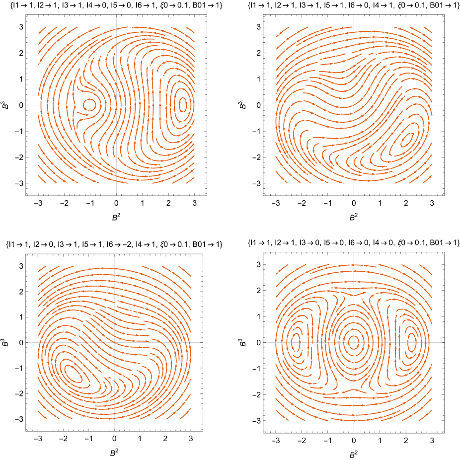
Figure 1: Phase space portrait for the system (35), (36) for different values of the free parameters. We observe that there are periodic solutions which indicates the existence of travel-wave solutions for the system.

3.2 Symmetry vector $X_{1}+X_{3}$

From the point symmetry vector $X_{1}+X_{3}$ we find

$$I_{1}=\rho u^{1}~{},~{}u^{2}=\frac{B_{0}^{1}B^{2}+I_{2}}{I_{1}}~{},~{}u^{3}=\frac{B_{0}^{1}B^{3}+I_{3}}{I_{1}}~{},$$ (37)

where $\rho=\rho\left(\sigma\right),~{}B^{2}=B^{2}\left(\sigma\right)~{},~{}B^{3}=B^{3}\left(\sigma\right),~{}$ $\sigma=x+\frac{t^{2}}{2}$ satisfy the following system of first-order ordinary differential equations

$$\rho_{,\sigma} = \frac{1}{\xi_{0}B_{0}^{1}I_{1}^{2}}\rho^{3}\left(\xi_{0}B_{0}^{1}+I_{5}B^{2}-I_{6}B^{3}\right)~{},~{}$$ (38)

$$B_{,\sigma}^{2} = \frac{1}{\xi_{0}B_{0}^{1}I_{1}}\left(I_{5}I_{1}\rho+\left(B_{0}^{1}\rho-I_{1}^{2}\right)B^{3}\right)~{},~{}$$ (39)

$$B_{,\sigma}^{3} = -\frac{1}{\xi_{0}B_{0}^{1}I_{1}}\left(I_{6}I_{1}\rho+\left(B_{0}^{1}\rho-I_{1}^{2}\right)B^{2}\right)~{}.$$ (40)

In analytic solution of the latter system can be written in terms of the Laurent expansion

$$\rho\left(\sigma\right) = \rho_{0}\sigma^{-\frac{1}{2}}+\rho_{1}\sigma^{-1}+\rho_{2}\sigma^{-\frac{3}{2}}+...~{},$$ (41)

$$B^{2}\left(\sigma\right) = B_{0}^{2}\sigma^{\frac{1}{2}}+B_{1}^{2}+B_{2}^{2}\sigma^{-\frac{1}{2}}+...~{},$$ (42)

$$B^{3}\left(\sigma\right) = B_{0}^{3}\sigma^{\frac{1}{2}}+B_{1}^{3}+B_{2}^{3}\sigma^{-\frac{1}{2}}+...~{},$$ (43)

in which $\rho_{0}=\frac{iI_{1}}{\sqrt{2}}~{},~{}B_{0}^{2}=\frac{i\sqrt{2}I_{1}}{B_{0}^{1}\xi_{0}}I_{5},~{}B_{0}^{3}=\frac{i\sqrt{2}I_{1}}{B_{0}^{1}\xi_{0}}I_{6},...$ .

The qualitative evolution of the dynamical variables $\rho,~{}B^{2}$ and $B^{3}$ are presented for various sets of initial conditions in Fig. 2. From the figure we observe a periodic behaviour on the dynamical variables.

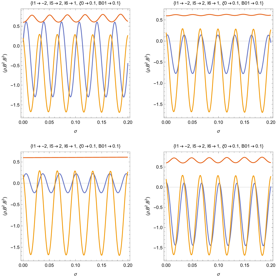
Figure 2: Qualitative evolution of the dynamical variables $\rho\left(\sigma\right)$ (red line),  $B^{2}\left(\sigma\right)$ (blue line) and $B^{3}\left(\sigma\right)$ (orange line) for different sets of the free variables. From the plots we observe a periodic solution, this is a new wave solution.

3.3 Symmetry vector $X_{7}$

Application of the symmetry vector $X_{7}$ in the system (4)-(9) provides the closed-form solution

$$\rho = \frac{\rho_{0}t+\rho_{1}}{x^{2}}~{},~{}u^{1}=\frac{\rho_{0}x}{\rho_{0}t+\rho_{1}}~{},~{}$$ (44)

$$u^{2} = \frac{u_{0}^{2}x}{\rho_{0}t+\rho_{1}}~{},~{}u^{3}=\frac{u_{0}^{3}x}{\rho_{0}t+\rho_{1}}~{},~{}$$ (45)

$$B^{2} = \frac{B_{0}^{1}u_{0}^{2}t+B_{0}^{2}}{\rho_{0}t+\rho_{1}}~{},~{}B^{2}=\frac{B_{0}^{1}u_{0}^{3}t+B_{0}^{3}}{\rho_{0}t+\rho_{1}}~{}.$$ (46)

3.4 Symmetry vector $X_{1}+aX_{7}$

From the vector field $X_{1}+aX_{7}$ we find $z=xe^{-\alpha t},~{}v=e^{-at}\mathbf{u~{},~{}}B^{2},B^{3},\mu=e^{-2at}\rho$, hence by replacing in (4)-(9) it follows

$$I_{1} = \rho v^{1}\left(v^{1}-az\right)+\frac{1}{2}\left(\left(B^{2}\right)+\left(B^{3}\right)^{2}\right)^{2}~{},$$ (47)

$$I_{2} = \rho v^{2}\left(v^{1}-az\right)-B_{0}^{1}B^{2}~{},$$ (48)

$$I_{3} = \rho v^{3}\left(v^{1}-az\right)-B_{0}^{1}B^{3}~{},$$ (49)

where $\rho\left(z\right),~{}B^{2}\left(z\right)$ and $B^{3}\left(z\right)$ satisfy the following system of ordinary differential equation

$$\left(\rho v^{1}-az\rho\right)_{,z}-az\rho = 0,$$ (50)

$$\left(B^{2}v^{1}-B_{0}^{1}v^{2}-\frac{\xi_{0}B_{0}^{1}}{\rho}B_{,z}^{2}\right)_{,z}-azB_{,z}^{2} = 0,$$ (51)

$$\left(B^{3}v^{1}-B_{0}^{1}v^{3}+\frac{\xi_{0}B_{0}^{1}}{\rho}B_{,z}^{3}\right)_{,z}-azB_{,z}^{3} = 0.$$ (52)

The qualitative evolution of the variables $\rho\left(z\right),~{}B^{2}\left(z\right)$ and $B^{3}\left(z\right)$ as it is given by the numerical simulation of the system (50)-(52) is presented in Fig. 3.

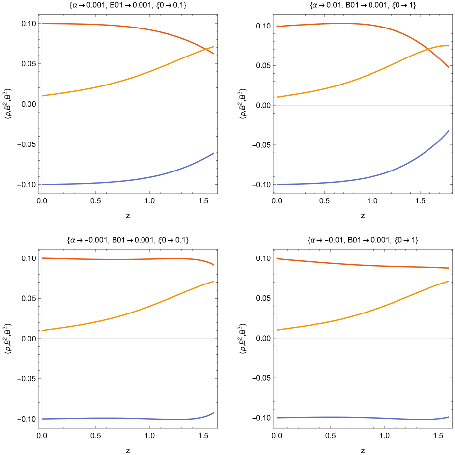
Figure 3: Numerical simulation and evolution of the dynamical variables $\rho\left(z\right)~{}$(red line)$,~{}B^{2}\left(z\right)$ (blue line) and $B^{3}\left(z\right)$ (orange line) as it is given by the system (50)-(52). The plots are for different values of the free parameter. For the initial conditions we considerered $\rho\left(0\right)=0.1$,$~{}B^{2}\left(0\right)=0.1$, $B^{3}\left(0\right)=-0.01$, $B_{,z}^{2}\left(0\right)=0.01,$ $B_{z}^{3}\left(0\right)=0.01,~{}v^{1}\left(0\right)=0.1,~{}v^{2}\left(0\right)=-0.02,~{}v^{3}\left(0\right)=0.2$.

3.5 Symmetry vector $X_{3}+aX_{6}$

From the Lie symmetry vector $X_{3}+X_{6}$ it follows

$$B^{2}\left(t,x\right) = -b^{2}\left(t\right)\cos\left(\frac{x}{t}\right)+b^{3}\left(t\right)\sin\left(\frac{x}{t}\right),$$

$$B^{3}\left(t,x\right) = b^{2}\left(t\right)\sin\left(\frac{x}{t}\right)+b^{3}\left(t\right)\cos\left(\frac{x}{t}\right),$$

$$u^{1}\left(t,x\right) = \frac{x}{t}+v^{1}\left(t\right),$$

$$u^{2}\left(t,x\right) = v^{2}\left(t\right)\sin\left(\frac{x}{t}\right)+v^{3}\cos\left(\frac{x}{t}\right)~{},$$

$$u^{3}\left(t,x\right) = v^{2}\left(t\right)\cos\left(\frac{x}{t}\right)-v^{3}\sin\left(\frac{x}{t}\right)~{},$$

$$\rho\left(t,x\right) = \rho\left(t\right),$$

while the 1D HMHD system (4)-(9) provides

$$\rho\left(t\right)=\rho_{0}t^{-1},~{}v^{1}\left(t\right)=v_{0}^{1}t^{-1}~{},$$ (53)

and

$${}_{0}v_{,t}^{2}-_{0}v_{0}^{1}t^{-2}v^{3}-B_{0}^{1}b^{2} = 0,$$ (54)

$$\rho_{0}v_{,t}^{3}+_{0}v_{0}^{1}t^{-2}v^{2}-B_{0}^{1}b^{3} = 0,$$ (55)

$$tb_{,t}^{2}-\frac{\xi_{0}B_{0}^{1}}{\rho_{0}}b^{3}+\left(B_{0}^{1}v^{2}+b^{2}-b^{3}v_{0}^{1}t\right) = 0,$$ (56)

$$tb_{,t}^{3}+\frac{\xi_{0}B_{0}^{2}}{\rho_{0}}b^{2}+\left(B_{0}^{1}v^{3}+b^{3}+b^{2}v_{0}^{1}t\right) = 0.$$ (57)

Consider the special case where $v_{0}^{1}=0$, then from the two first equation of the latter system it follows $b^{2}=\frac{{}_{0}}{B_{0}^{1}}v_{,t}^{2}$ and $b^{3}=\frac{{}_{0}}{B_{0}^{3}}v_{,t}^{3}$. Thus by replacing in the rest two equations we find

$$t\frac{{}_{0}}{B_{0}^{1}}v_{,tt}^{2}-\left(\xi_{0}-\frac{{}_{0}}{B_{0}^{1}}\right)v_{,t}^{2}+B_{0}^{1}v^{2} = 0~{},$$ (58)

$$t\frac{{}_{0}}{B_{0}^{1}}v_{,tt}^{3}+\left(\xi_{0}+\frac{{}_{0}}{B_{0}^{1}}\right)v_{,t}^{3}+B_{0}^{1}v^{3} = 0~{},$$ (59)

with solution which can expressed in terms of the Bessel functions $J_{\alpha}\left(t\right)$ and $Y_{\alpha}\left(t\right)$. Note that for $v_{0}^{1}\neq 0$ system (54)-(57) can be written into the form of an equivalent system of two linear second-order ordinary differential equations which means that the system is integrable.

In Fig. 4 we present the numerical solution of the dynamical system (54)-(57) while some phase space portraits are given in Fig. 5. It is clear that the behaviour is of the dynamical variables has oscillations for $v_{0}^{1}$ and $B_{0}^{1}$ positive.

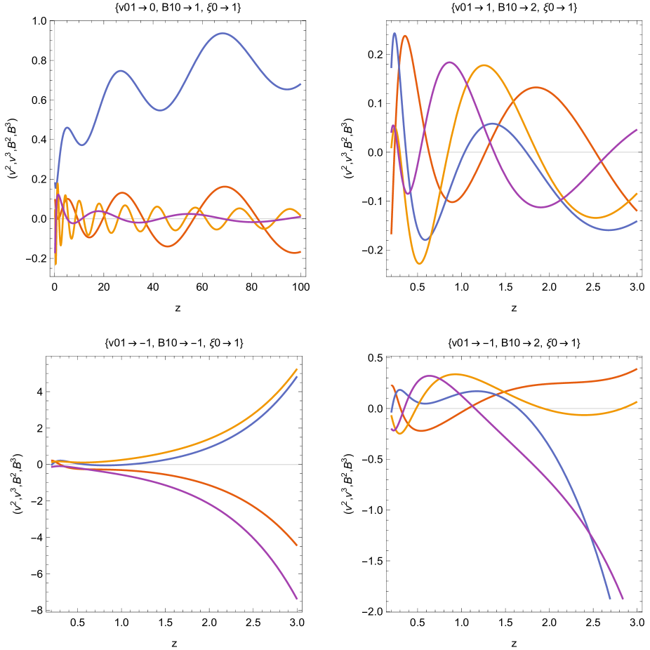
Figure 4: Numerical simulation and evolution of the dynamical variables $v^{2}\left(t\right)~{}$(red line)$,~{}v^{3}\left(t\right)~{}$(blue line) $b^{2}\left(z\right)$ (orange line) and $b^{3}\left(z\right)$ (purple line) as it is given by the system (54)-(57). The plots are for different values of the free parameter.

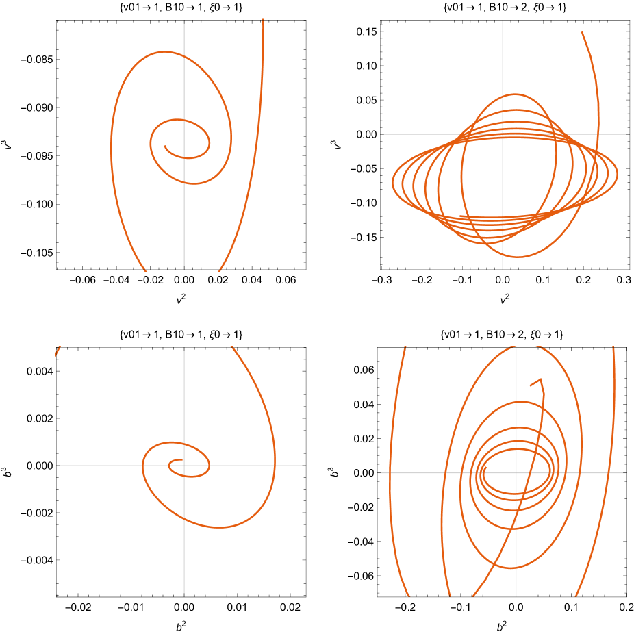
Figure 5: Phase space portraits on the variables $\left\{v^{2}-v^{3}\right\}$ and $\left\{b^{2}-b^{3}\right\}$ for the oscillating solutions of Fig. 4

4 Conclusions

In this work we studied the group properties the nonlinear one-dimensional system of MHD included the Hall term. The dynamical system is consisted by six 1+1 partial differential equations. For this system, we applied the theory of Sophus Lie and we determined all the possible one-parameter point transformations in which the HMHD equations are invariant. We found that the admitted Lie point symmetries form a seven dimensional Lie algebra. The admitted Lie algebra has common element with that of the MHD system without the Hall term, thus it admits a smaller number of Lie symmetries for the equivalent system without the Hall term.

For the admitted Lie symmetries we calculated the commutators and the Adjoint representations as also the adjoint invariants. These results were applied in order to determine all the one-dimensional Lie algebras which consisted the optimal system. We found that the one-dimensional system is consisted by thirty five independent vector fields. For the latter vector fields the invariant functions which define the similarity transformations were determined which are applied for the definition of the similarity transformations.

Furthermore, we applied the Lie point symmetries to reduce the partial differential equations into a system of ordinary differential equations and to study the behaviour of the dynamical variables. Travel-wave and scaling solutions were found.

These results contribute to the subject of the application of the Lie point symmetries to fluid dynamics and specifically on MHD.

References

- [1] A.A. Chesnokov, Eur. J. Appl. Math. 20, 461 (2009)
- [2] X. Xin, L. Zhang, Y. Xia and H. Liu, Appl. Math. Lett. 94, 112 (2019)
- [3] S. Szatmari and A. Bihlo, Comm. Nonl. Sci. Num. Sim. 19, 530 (2014)
- [4] A.A. Chesnokov, J. Appl. Mech. Techn. Phys. 49, 737 (2008)
- [5] J.-G. Liu, Z.-F. Zeng, Y. He and G.-P. Ai, Int. J. Nonl. Sci. Num. Sim. 16, 114 (2013)
- [6] M. Pandey, Int. J. Nonl. Sci. Num. Sim. 16, 93 (2015)
- [7] A. Paliathanasis, Zeitschrift fur Naturforschung A 74, 869 (2019)
- [8] A. Paliathanasis, Symmetry 11, 1115 (2019)
- [9] V.A. Dorodnitsym and E.I. Kaptsov, Comm. Nonl. Sci. Num. Sim. 89, 105343 (2020)
- [10] S.V. Meleshko and N.F. Samatova, Comm. Nonl. Sci. Num. Sim. 90, 105337 (2020)
- [11] S.V. Meleshko, Comm. Nonl. Sci. Num. Sim. 89, 105293 (2020)
- [12] A. Bihlo, N. Poltavets and R.O. Popovych, Chaos 30, 073132 (2020)
- [13] D. Zeidan and B. Bira, Math. Meth. Appl. Sci. 42, 4679 (2019)
- [14] B. Bira, T.S. Raja and D. Zeidan, Comput. Math. Appl. 71, 46 (2016)
- [15] B. Bira, T.S. Raja and D. Zeidan, Math. Meth. Appl. Sci. 41, 6717 (2018)
- [16] P.Y. Picard, J. Math. Anal. Appl. 337, 360 (2008)
- [17] A.B. Rosmila, R. Kandasamy and I. Muhaimin, Appl. Math. Mech. 33, 593 (2012)
- [18] S.M. Moawad, Eur. Phys. J. Plus 135, 585 (2020)
- [19] G.M. Webb, G.P. Zank, E. Kh. Kaghashvili and R.E. Ratkiewicz, J. Plasma Physics 71, 785 (2005)
- [20] G.M. Webb, G.P. Zank, E. Kh. Kaghashvili and R.E. Ratkiewicz, J. Plasma Physics 71, 811 (2005)
- [21] G.M. Webb and G.P. Zank, J. Phys. A: Math. Theor. 40, 545 (2006)
- [22] G.M. Webb and S.C. Anco, AIP Conf. Proc. 2153, 020024 (2019)
- [23] A. Paliathanasis, Math. Meth. App. Sc. 43, 716 (2020)
- [24] D. Biskamp, Nonlinear Magnetohydrodynamics, Cambridge University Press, Cambridge (1993)
- [25] E.A. Witalis, IEEE Transactions on Plasma Science PS-14 842 (1986)
- [26] H.M. Abdelhamid, M. Lingam and S.M. Mahajan, Astrophysical J. 829, 87 (2016)
- [27] D.O. Gómez, Proceedings of the International Astronomical Union 6, 433 (2010)
- [28] Z. Ye, Applicable Analysis 96, 2669 (2017)
- [29] V.V. Savelyev, Journal of Physics: Conf. Series 1094, 012031 (2018)
- [30] A. Rogister, Phys. Fluids 14, 2733 (1971)
- [31] E. Mjolhus and J. Willer, Physica Scripta 33, 442 (1986
- [32] K. Mio, K.T. Minami and S. Takeda, J. Phys. Soc. Japan 41, 265 (1976)
- [33] D.J. Kaup and A.C. Newell, J. Math. Phys. 19, 798 (1978)
- [34] G.M. Webb, M. Brio and G.P. Zank, Journal of Plasma Physics 54, 201 (1995)
- [35] Z. Yoshida and E. Hameiri, J. Phys. A: Math. Theor. 46, 335502 (2013)
- [36] E.C. D’Avignon, P.J. Morrrison and M. Lingam, Physics of Plasmas 23, 062101 (2016)
- [37] P.J. Olver, Applications of Lie Groups to Differential Equations, Springer-Verlag, New York, (1993)
- [38] G.W. Bluman and S. Kumei, Symmetries and Differential Equations, Springer-Verlag, New York, (1989)
- [39] N.H. Ibragimov, CRC Handbook of Lie Group Analysis of Differential Equations, Volume I: Symmetries, Exact Solutions, and Conservation Laws, CRS Press LLC, Florida (2000)