[2105.10317] Supplemental Materials for On the use of feature-maps and parameter control for improved quality-diversity meta-evolution

S1 Experimental parameters

For convenience, Table S1 includes all the parameter settings for the experimental setup.

Table S1: Parameter settings for evolution. Top half shows settings common to all conditions while bottom half shows settings for Meta-conditions.

Parameter	Setting
Genotype ( $\mathbf{g}$ )	discretised in $[0,1]^{8}$
Mutation rate	$0.125$ (unless otherwise indicated)
Mutation type	random increment/decrement with step of $0.025$
Maximal map coverage	4,096 solutions
Function evaluations	100,000,000
Batch size per generation	400 bottom-level individuals
Initial population ( $p$ )	2,000 bottom-level individuals
Meta-population size ( $\lambda$ )	5
Meta-genotype ( $\mathbf{w}$ )	$[-1,1]^{182}$ for non-linear feature-map $[0,1]^{56}$ otherwise
Number of base-features ( $N_{b}$ )	14
Number of target-features ( $D$ )	4
Normalisation range ( $[m,M]$ )	$[0.20,0.80]$ (linear feature-maps)
Number of hidden units ( $N_{h}$ )	10 (non-linear feature-maps)
Sigmoid scaling factor ( $\alpha_{s}$ )	30 (non-linear feature-maps)
Database settings	initial $k=5000$ ; bin width $\delta=1/3$ ; capacity $3^{14}$ (just below 5 million)

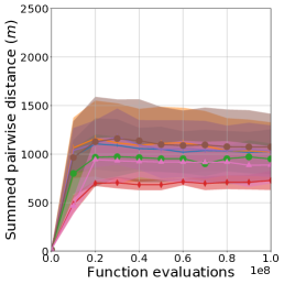
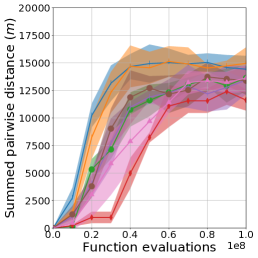
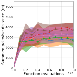
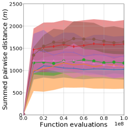
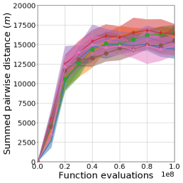
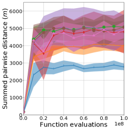
S2 Meta-fitness development

This section provides more data on the development of meta-fitness, the summed pairwise distance across 10% of solutions in the map. Table S2 displays the final meta-fitness of Meta-evolution algorithms as a function of parameter control strategy. Fig. S1 illustrates the effect of controlling the number of generations per meta-generations, with one separate plot for each feature-map (linear, non-linear, and feature-selection). Fig. S2 analogously illustrates the effect of controlling the mutation rate for different feature-maps.

Table S2: Comparison of parameter control methods. The data are divided into 6 groups based on the type of feature-map and the parameter controlled, either the number of generations or the mutation rate. Within each group, bold highlights the condition with highest meta-fitness. Final meta-fitness is is averaged over the final 10% (i.e., the final 10 million) function evaluations.

Parameter control	Meta-fitness
5 generations	$1037.7\pm 215.9$
10 generations	$1037.9\pm 310.8$
25 generations	$952.3\pm 168.7$
50 generations	$718.8\pm 86.0$
Annealing generations	$1036.0\pm 262.9$
RL generations	$\mathbf{1088.7\pm 373.4}$
Endogenous generations	$886.2\pm 207.6$
Mutation rate 0.125	$1037.7\pm 215.9$
Mutation rate 0.25	$1093.7\pm 499.7$
Mutation rate 0.50	$1185.0\pm 258.7$
Mutation rate 1.0	$1581.3\pm 531.4$
Annealing mutation rate	$1292.4\pm 435.6$
RL mutation rate	$\mathbf{1640.5\pm 340.1}$
Endogenous mutation rate	$1113.2\pm 266.4$

(a) Linear feature-map

Parameter control	Meta-fitness
5 generations	$14562.2\pm 1084.8$
10 generations	$\mathbf{14716.5\pm 847.5}$
25 generations	$13282.5\pm 1276.7$
50 generations	$12014.3\pm 1020.3$
Annealing generations	$12985.3\pm 1697.6$
RL generations	$13442.5\pm 868.1$
Endogenous generations	$13390.7\pm 1034.7$
Mutation rate 0.125	$14562.2\pm 1084.8$
Mutation rate 0.25	$\mathbf{16470.0\pm 653.6}$
Mutation rate 0.50	$16327.3\pm 785.0$
Mutation rate 1.0	$16431.4\pm 1459.5$
Annealing mutation rate	$15292.1\pm 1198.2$
RL mutation rate	$15054.2\pm 1365.9$
Endogenous mutation rate	$14574.3\pm 1447.8$

(b) Non-linear feature-map

Parameter control	Meta-fitness
5 generations	$2719.1\pm 149.0$
10 generations	$3009.4\pm 745.4$
25 generations	$2795.7\pm 515.0$
50 generations	$\mathbf{3817.6\pm 520.2}$
Annealing generations	$3356.3\pm 442.1$
RL generations	$3701.7\pm 662.2$
Endogenous generations	$3198.0\pm 729.0$
Mutation rate 0.125	$2719.1\pm 149.0$
Mutation rate 0.25	$4050.7\pm 350.1$
Mutation rate 0.50	$\mathbf{5067.7\pm 263.2}$
Mutation rate 1.0	$4755.9\pm 982.5$
Annealing mutation rate	$4896.3\pm 1019.3$
RL mutation rate	$4901.4\pm 739.8$
Endogenous mutation rate	$4781.6\pm 449.3$

(c) Selection feature-map

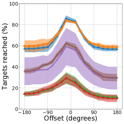
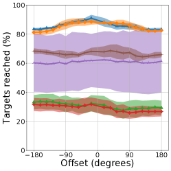
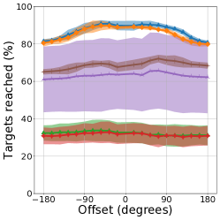
S3 Test comparison of meta-conditions

This section provides additional data about the performance of the meta-conditions as they are tested on unseen damages, which offset the desired angle by a particular error in $[-180,180]$ degrees. Table S3 shows summary and significance statistics of damage recovery, with data being aggregated across all offsets. Fig. S3 presents the damage recovery for two selected joints as the offset is varied.

Table S3: Summary statistics of test on unseen damages. For each meta-condition, we show the percentage of targets reached within the semi-circle span of the robot and, to assess the effect compared to Meta NonLinear (Optimised), the Wilcoxon rank-sum test’s significance value and Cliff’s delta as an effect size. Bold highlights large effect sizes. The behaviour-performance map is generated from the mean meta-genotype (see

\mathbf{m}

in Eq. 5). Default parameter settings are a mutation rate of

0.125

and 5 generations per meta-generation. Optimised indicates the best setting from parameter control: RL mutation rate for Meta Linear, Mutation rate 0.25 for Meta NonLinear, and Mutation rate 0.50 for Meta Selection.

Condition	Targets reached ( $\%$ )	Significance	Cliff’s delta
Meta NonLinear (Optimised)	$79.16\pm 11.38$	/	/
Meta NonLinear	$79.10\pm 10.66$	$p=0.338$	$0.03$
Meta Selection (Optimised)	$26.86\pm 8.02$	$p<0.001$	$\mathbf{1.00}$
Meta Selection	$25.82\pm 7.80$	$p<0.001$	$\mathbf{1.00}$
Meta Linear (Optimised)	$54.85\pm 21.13$	$p<0.001$	$\mathbf{0.72}$
Meta Linear	$59.35\pm 12.50$	$p<0.001$	$\mathbf{0.74}$

S4 Source code

Source code for the experiments is publicly available at https://github.com/resilient-swarms/planar_metacmaes.