Shear dynamics of confined membranes

Abstract

We model the nonlinear response of a lubricated contact composed of a two-dimensional lipid membrane immersed in a simple fluid between two parallel flat and porous walls under shear. The nonlinear dynamics of the membrane gives rise to a rich dynamical behavior depending on the shear velocity. In quiescent conditions (i.e., absence of shear), the membrane freezes into a disordered labyrinthine wrinkle pattern. We determine the wavelength of this pattern as a function of the excess area of the membrane for a fairly general form of the confinement potential using a sine-profile ansatz for the wrinkles. In the presence of shear, we find four different regimes depending on the shear rate. Regime I. For small shear, the labyrinthine pattern is still frozen, but exhibits a small drift which is mainly along the shear direction. In this regime, the tangential forces on the walls due to the presence of the membrane increase linearly with the shear rate. Regime II. When the shear rate is increased above a critical value, the membrane rearranges, and wrinkles start to align along the shear direction. This regime is accompanied by a sharp drop of the tangential forces on the wall. The membrane usually reaches a steady-state configuration drifting with a small constant velocity at long times. However, we also rarely observe oscillatory dynamics in this regime. Regime III. For larger shear rates, the wrinkles align strongly along the shear direction, with a set of dislocation defects which assemble in pairs. The tangential forces are then controlled by the number of dislocations, and by the number of wrinkles between the two dislocations within each dislocation pairs. In this dislocation-dominated regime, the tangential forces in the transverse direction most often exceed those in the shear direction. Regime IV. For even larger shear, the membrane organizes into a perfect array of parallel stripes with no defects. The wavelength of the wrinkles is still identical to the wavelength in the absence of shear. In this final regime, the tangential forces due to the membrane vanish. These behaviors give rise to a non-linear rheological behavior of lubricated contacts containing membranes.

I Introduction

Biolubrication is vital for the function of biological organs of living species. One of the key ingredients of biolubricating systems is lipid membranes, which reduce the friction coefficient and wear of rubbing surfaces Trunfio-Sfarghiu et al. (2008). An example of biolubrication system is synovial fluid confined between opposing cartilage surfaces within the joints of human and other animals. Synovial fluid has three important components: surface-active phospholipids, hyaluronan (acid) and proteoglycan-4 (proteins) Schmidt et al. (2007). In synovial fluids, surface-active phospholipids form stacks of parallel bilayers at the surface of the cartilage, which reduce the friction coefficient Botan et al. (2015). Swann et al. Swann et al. (1984) suggest that the response of synovial fluids to friction is related to joint diseases such as degeneration, traumatic injury, inflammation, infection, acute gout syndrome, and arthritis. In another study for knee joint, Tadmor et al. Tadmor et al. (2002) proposed that the combination of synovial membrane, ligament, tendon and skin acts together like a spring between opposing cartilages and applies tensile force on the joint as one lifts his or her leg. In contrast the presence of hyaluronan helps to slow down the compression between cartilages as one puts weight on the joint.

The role of parallel lipid bilayers to reduce the friction coefficient at biological surfaces such as cartilage has prompted several groups to cover model artificial surfaces with lipid bilayers, thereby reducing the friction coefficient to very low values around $10^{-3}$ Trunfio-Sfarghiu et al. (2008). These results suggest novel routes towards applications in the automotive and manufacturing industry where more effective and efficient lubrications are in high demand in order to save fuel, increase engine durability, and reduce environmental pollution. These industrial criteria of lubrication systems may be achieved by the development and consumption of low friction materials, coatings, and lubricants Erdemir (2005). In addition, the study of friction in model lubrication system may have implications for the lubrication of biomedical devices and microelectromechanical systems and suggests applications in living systems Raviv et al. (2003); Briscoe et al. (2006).

In the past decades, many studies have focused on the dynamics of stacks of membranes under shear (see, e.g., Ref.Gov et al. (2004) and references therein). They have pointed out the instabilities of these stacks induced by shear, and the stabilizing effect or shear on thermal fluctuations of the membranesMarlow and Olmsted (2002). In this paper we investigate a simple situation where a single membrane sandwiched between two porous walls. We focus on wrinkling patterns formed by membranes due to their excess area, and show that the nonlinear dynamics of these wrinkles gives rise to a rich rheological behavior. Wrinkle patterns have been observed in many systems where thin films are present such as stressed thin films on soft substrate Huang and Im (2006), confined liquid membranes To et al. (2018), stretched polyethylene sheets Cerda and Mahadevan (2003) or confined biogel membranes Leocmach et al. (2015). In the first two cases Huang and Im (2006); To et al. (2018), the thin film forms sinusoidal wavelike patterns with a characteristic wavelength and the wrinkles meander to form the isotropic labyrinthine patterns Le Berre et al. (2002).

Our work extends our previous study in one dimension Le Goff et al. (2017). Here, we consider a lubricated contact containing a two-dimensional membrane immersed in a Newtonian fluid between two flat permeable walls. These permeable walls account for porous materials such as the collagen of the cartilage matrix in joints, or the cytoskeleton which is in contact with membranes in biological cells. The walls move with constant and opposite velocities leading to a shear flow. We find that, while confinement of the membrane gives rise to the formation of wrinkles that store the excess area, shear can rearrange these wrinkles. The membrane then experiences nontrivial configurations, which lead to a back-flow that produces tangential forces on the confining walls. These tangential forces exhibit a nonlinear dependence on the shear rate, and therefore give rise to a complex nonlinear rheological response of the lubricated contact.

In the following, we first present the lubrication model in Section 2. We consider a two-dimensional inextensible membrane with bending rigidity in a simple liquid between two flat and permeable walls. We describe the wall-substrate with a generic membrane-wall potential that diverges as the membrane approaches the wall, thereby preventing the membrane from crossing the walls (this is in contrast with harmonic potentials, such as that used e.g. in Ref. Gov et al. (2004)).

In section 3, we investigate the dynamics in the absence of shear. We find that the wrinkles relax to a steady-state composed of a labyrinthine pattern of wrinkles. A sine-ansatz profile provides a quantitative prediction for the width of the wrinkles.

Section 4 is devoted to the numerical investigation of the membrane dynamics in the presence of shear, and of the resulting tangential forces acting on the walls. We find four different regimes as a function of the shear rate. In regime I, the membrane exhibits a labyrinthine pattern that is similar to that found in the absence of shear. However, the membrane exhibits a small drift, mainly oriented along the shear direction. The forces due to the presence of the membrane then increase linearly with the shear rate. When the shear rate exceeds a critical value $\upsilon_{c}$, the membranes start to rearrange, and align partially along the shear direction. We denote this regime as Regime II. In regime II, the forces on each wall drop sharply. We have also sometimes observed oscillatory dynamics in regime II. Further increase of the shear rate leads to regime III, where wrinkles are strongly ordered along the shear direction. In regime III, dislocations can be observed. These dislocations form pairs. In this regime, the tangential forces exhibit a complex dependence on the shear rate, and the tangential forces in the transverse direction are found to be often larger than in the shear direction. Finally, for very large shear rate, the dislocations disappear and the membrane exhibits a perfect array of wrinkles parallel to the shear direction. In this regime, hereafter denoted as regime IV, the tangential forces vanish.

In section 5, we determine the critical velocity $\upsilon_{c}$ from a balance between the shear term and the other terms in the dynamical equations. Section 6 is devoted to the analysis of the tangential force on the walls. For small shear rate in regime I, we use the sine anstaz to obtain a quantitative prediction of the tangential forces. Furthermore, we show that the total force acting on the walls can be decomposed as a sum of contributions of dislocation pairs in regime III. In Section 7, we claim that the transition to regime IV is controlled by finite size effects. Finally, a summary and discussion of our results are presented in Section 8.

II Model

II.1 Evolution equation for a confined membrane under shear

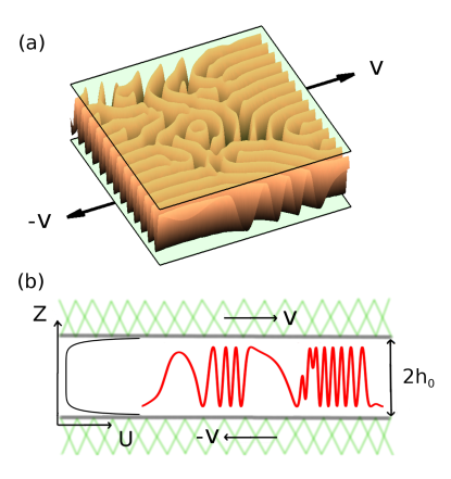
Figure 1: Membrane between two repulsive substrates. For the sake of clarity, the vertical scale is strongly magnified in (a) and (b) (our analysis applies in the limit where the vertical scale is much smaller than the horizontal scale, i.e., when slopes are small). Profiles in (a) and (b) are obtained from simulation with $\Delta A_{*}=0.1503$, $V=2$ at $T=4\times 10^{5}$. (a) 3D view; (b) 2D view, left black curve: membrane-walls interaction potential, right red curve: a section of the membrane profile.

In previous papers, we have contributed to the modeling of the dynamics of membranes placed between two walls, with Le Goff et al. (2017) or without To et al. (2018) shear. Beyond the presence of shear induced by the motion of the walls, two main physical ingredients of the models can be used to categorize the dynamics that we have investigated so far.

The first ingredient is the interaction of the membrane with the walls. The interaction of the membrane with one wall can be dominated by purely repulsive interactions, such as hydration interactions Swain and Andelman (2001), or repulsion due to polymer brushes Sengupta and Limozin (2010). When attractive forces are present, such as those induced at long range by van der Waals force Israelachvili (2015), or at short distances by molecular binders  Sengupta and Limozin (2010), one obtains a potential well for the membrane at a distance $h_{w}$ from a wall. If the walls are attractive and if the distance between the two walls is larger than $h_{w}$, then the potential experienced by the membrane exhibits a double-well profile. In contrast, if the interaction is purely repulsive or if the interaction is attractive but the distance between the two walls is smaller than or similar to $2h_{w}$, then the membrane experiences a single-well potential. Single and double-well potentials give rise to different membrane behaviors. For example in the absence of shear, coarsening of adhesion domains coexisting with wrinkles can be observed with double-well potentials as discussed in Ref. To et al. (2018), while only frozen labyrinthine wrinkle patterns can be seen with single-well potentials, as discussed below.

The second ingredient is the balance between two dissipation mechanisms, controlled by the viscosity of the liquid and the permeability of the walls. The relative roles of the liquid flow through the walls and along the walls is characterized by a dimensionless number To et al. (2018)

$$\bar{\nu}=12\frac{\kappa^{1/2}\mu\nu}{\mathcal{U}_{0}^{1/2}h_{0}^{2}}.$$ (1)

Here, $\kappa$ is the bending rigidity of the membrane, $\mu$ is the viscosity of the fluid surrounding the membrane, $\nu$ is a kinetic coefficient describing the permeability of the wall, $\mathcal{U}_{0}$ is an energy scale for the adhesion potential, and $2h_{0}$ is the distance between the two walls. In this work we focus on the limit of very large permeability $\bar{\nu}\gg 1$, but where viscosity and hydrodynamic flows along the membrane are still relevant. This limit which aims at describing membranes sandwiched between porous biological substrates such as collagen or the cytoskeleton, is discussed quantitatively in more details in section VIII.1 and Ref. To et al. (2018). The opposite limit of impermeable walls $\bar{\nu}\ll 1$ is suitable to describe, e.g., substrates covered by other lipid membranes as discussed in Ref. To et al. (2018). Models which account for finite permeability $\bar{\nu}\sim 1$ have also been reported in Ref. To et al. (2018).

The effect of shear on membrane dynamics with impermeable walls and a double-well potential has been investigated in our previous work in Ref. Le Goff et al. (2017) within a one-dimensional model. In this work, we focus on the case of permeable walls with a single-well potential within a two-dimensional model.

More precisely, we consider the dynamics of a two-dimensional membrane confined between two walls at height $\pm h_{0}$ moving at constant velocities $\pm\upsilon_{0}$. A three-dimensional representation of the membrane and the walls is shown in Fig. 1(a and b). The walls are permeable with a permeability constant $\nu$. Within the small-slope approximation, the evolution equation for the membrane was derived in one dimension with shear in Ref.Le Goff et al. (2017), and in two dimensions without shear in Ref.To et al. (2018). The combination of these models to obtain a two-dimensional model with shear is straightforward. Here, we do not report the full derivation, but we motivate the different terms appearing in the equations.

In the limit of large permeability, i.e. when $\bar{\nu}$ is large, an equation governing the membrane height $h(x,y)$ can be obtained from the lubrication (small slope) limit. The main ingredients of the derivation are reported in Appendix A, while more details are provided in Ref. To et al. (2018). This equation takes a simple form

$$\partial_{t}h=\frac{\nu}{2}f_{z}-\frac{\upsilon_{0}}{h_{0}}h\partial_{x}h,$$ (2)

where $x$-axis is parallel to the shear direction and $f_{z}$ accounts for the internal forces on the membrane along the $z$ direction orthogonal to the walls

$$f_{z}=-\kappa\Delta^{2}h+\sigma_{0}\Delta h-{\cal U}^{\prime}(h),$$ (3)

where $\kappa$ is the bending rigidity Canham (1970); Helfrich (1973) of the membrane. The term $\sigma_{0}$ is a nonlocal tension which enforces a constant membrane area. Membrane tension usually accounts for the entropic tension of the membrane due to thermal fluctuationsLipowsky (1995); Seifert (1995), as well as some possible amount of finite membrane extensibility. Following Refs.Young et al. (2014); To et al. (2018); Le Goff et al. (2017), the tension here emerges to leading order in the dynamics of the membrane at small slopes as a result of the constraint of local inextensibility. Inserting the membrane excess area in the small slope limit

$$\Delta{\cal A} =\int_{0}^{{\cal L}_{x}}dx\int_{0}^{{\cal L}_{y}}dy\frac{1}{2}(\nabla h)^{2},$$ (4)

into Eq. (2), the membrane area conservation condition $\partial_{t}\Delta{\cal A}=0$ provides the expression of the tension of the membrane

$$\sigma_{0}=\frac{\int_{0}^{{\cal L}_{x}}dx\int_{0}^{{\cal L}_{y}}dy\left\{\left[\frac{\nu}{2}\left(\kappa\Delta^{2}h+{\cal U}^{\prime}(h)\right)+(\upsilon_{0}/h_{0})h\partial_{x}h\right]\Delta h\right\}}{\int_{0}^{{\cal L}_{x}}dx\int_{0}^{{\cal L}_{y}}dy\left\{\frac{\nu}{2}\left(\Delta h\right)^{2}\right\}}.$$ (5)

Finally, ${\cal U}$ is the confinement potential, i.e., the free energy for placing the membrane at the height $h$. This potential accounts for the interaction of the membrane with the porous walls. The walls account for the confinement of the membrane induced by the cytoskeleton of the cell Sheetz (2001); Speck and Vink (2012), or a biological substrate Maciver (1992); Berrier and Yamada (2007), or other membranes Braga (2002); Asfaw et al. (2006). We use a generic potential of the form

$${\cal U}(h)=\frac{{\cal U}_{0}}{[1-(h/h_{0})^{p}]^{m}}$$ (6)

with $m,p>0$, and $p$ even. Such a confinement potential allows one to account simultaneously for a divergence at the walls ${\cal U}(h)\approx{\cal U}_{0}p^{-m}(1\pm(h/h_{0}))^{-m}$ when $h\rightarrow\pm h_{0}$ with an arbitrary power $m$, and for a small amplitude behaviour ${\cal U}(h)\approx{\cal U}_{0}+m{\cal U}_{0}(h/h_{0})^{p}$ when $h\rightarrow 0$ with arbitrary power $p$.

II.2 Forces of the walls

The expression of the tangential forces on the walls generalizes the results of Ref. Le Goff et al. (2017) derived within a one-dimensional model in the limit of small slopes. These forces originate in the shear stress exerted by the fluid on the walls. For two-dimensional membranes, the force on each wall is opposite to the force on the other wall. A detailed derivation of these forces is reported is Appendix A. The two components of the force per unit area on one wall along the direction $x$ and $y$ are

$$f_{wx}=\frac{\mu}{h_{0}}\upsilon_{0}+f_{\mathrm{mem},x} f_{wy}=f_{\mathrm{mem},y}$$ (7)

The first contribution $\upsilon_{0}\mu/h_{0}$ is the viscous friction force due to the simple shear of the fluid along $x$ in the absence of membrane. The second contribution is due to the presence of the membrane

$$f_{\mathrm{mem},x}=\frac{1}{2{\cal L}_{x}{\cal L}_{y}}\int_{0}^{{\cal L}_{x}}dx\int_{0}^{{\cal L}_{y}}dy\left\{\frac{h_{0}}{2}\left(1-\frac{h^{2}}{h_{0}^{2}}\right)\partial_{x}f_{z}\right\},$$

$$f_{\mathrm{mem},y}=\frac{1}{2{\cal L}_{x}{\cal L}_{y}}\int_{0}^{{\cal L}_{x}}dx\int_{0}^{{\cal L}_{y}}dy\left\{\frac{h_{0}}{2}\left(1-\frac{h^{2}}{h_{0}^{2}}\right)\partial_{y}f_{z}\right\}.$$ (8)

A qualitative discussion of these expressions follows. In the lubrication limit, each flow above or below the membrane is a Poiseuille flow parallel to the walls $\upsilon_{x,y}$. These flows contribute to the tangential friction forces between the two walls when they produce viscous shear stresses $-\mu\partial_{z}\upsilon_{x,y}|_{h=h_{0}}$ on the upper wall and $+\mu\partial_{z}\upsilon_{x,y}|_{h=-h_{0}}$ on the lower wall which exhibit opposite signs, i.e., when $\partial_{z}\upsilon_{x,y}|_{h=h_{0}}$ and $\partial_{z}\upsilon_{x,y}|_{h=-h_{0}}$ have the same sign. This corresponds typically to an antisymmetric flow, with the property $\upsilon_{x,y}(z)=-\upsilon_{x,y}(-z)$. The first antisymmetric contribution to the flow is the average shear flow $\upsilon_{x,y}(z)=\upsilon_{0}z/h_{0}$ due to the imposed motion of the walls. This contribution gives rise to the first term in Eq. (7). In addition, the membrane normal force $f_{z}$ produces a difference of pressure between the fluids above and below the membrane. Spatial variations of $f_{z}$ therefore produce pressure gradients that give rise to additional fluid flow. This additional fluid flow is at the origin of the contributions $f_{\mathrm{mem},x}$ and $f_{\mathrm{mem},y}$ in Eq. (II.2). At this point, two important remarks should be made. First, the average flow on one side of the membrane vanishes when the membrane approaches the wall, due to an increase of viscous dissipation. Second, each flow above and below the membrane is a Poiseuille flow which cannot be antisymmetric by itself. As a consequence of these two properties, (i) the most antisymmetric flow is produced by placing the membrane in the middle of the cell and (ii) when the membrane is placed close to one wall, the flow is then essentially a symmetric Poiseuille. This is at the origin of the factor $1-h^{2}/h_{0}^{2}$ in Eq. (II.2), which is maximum when $h=0$ and vanishes when $h\rightarrow\pm h_{0}$.

Following the same lines as in Eq. (19) of Ref. Le Goff et al. (2017), we use periodic boundary conditions to rewrite the membrane contribution to the forces as

$$f_{\mathrm{mem},x}=\frac{1}{2h_{0}{\cal L}_{x}{\cal L}_{y}}\int_{0}^{{\cal L}_{x}}dx\int_{0}^{{\cal L}_{y}}dy(h\partial_{x}hf_{z}),$$

$$f_{\mathrm{mem},y}=\frac{1}{2h_{0}{\cal L}_{x}{\cal L}_{y}}\int_{0}^{{\cal L}_{x}}dx\int_{0}^{{\cal L}_{y}}dy(h\partial_{y}hf_{z}).$$ (9)

II.3 Normalization

We define the normalized time $T=t/t_{0}$, where

$$t_{0}=\frac{2h_{0}^{2}}{\nu\mathcal{U}_{0}},$$ (10)

the normalized height $H=h/h_{0}$, and the normalized space variables parallel to the walls $(X,Y)=(x,y)/\ell_{\parallel}$, where

$$\ell_{\parallel}=\left(\frac{\kappa h_{0}^{2}}{\mathcal{U}_{0}}\right)^{1/4}$$ (11)

accounts for the lengthscale in the $(x,y)$ plane on which a membrane placed away from the center between the walls decays back to the center in the linear approximation, i.e. in a harmonic potential. Since we consider the lubrication limit (small slopes), we assume that

$$\epsilon=\frac{h_{0}}{\ell_{\parallel}}\ll 1.$$ (12)

We also define the normalized shear velocity

$$V=\frac{\upsilon_{0}}{\upsilon_{\parallel}},$$ (13)

where

$$\upsilon_{\parallel}=\frac{\ell_{\parallel}}{t_{0}}=\frac{\nu\mathcal{U}_{0}^{3/4}\kappa^{1/4}}{2h_{0}^{3/2}}.$$ (14)

This leads to the normalized evolution equation

$$\partial_{T}H=F_{Z}-VH\partial_{X}H.$$ (15)

The normalized forces on the membrane then read

$$F_{Z}=-\Delta^{2}H+\Sigma_{0}\Delta H-U^{\prime}(H),$$ (16)

where

$$\Sigma_{0}=\frac{\int_{0}^{L_{X}}dX\int_{0}^{L_{Y}}dY\left\{\left[\left(\Delta^{2}H+U^{\prime}(H)\right)+VH\partial_{X}H\right]\Delta H\right\}}{\int_{0}^{L_{X}}dX\int_{0}^{L_{Y}}dY\left\{\left(\Delta H\right)^{2}\right\}},$$ (17)

and the normalized potential reads

$$U(H)=\frac{1}{(1-H^{p})^{m}}.$$ (18)

The changes in the shape of the normalized potential are reported in Fig. 2.

While analytical results will be discussed for arbitrary values of $p$ and $m$, we have focused on the case $m=1$ and $p=8$ in the numerical simulations. This rather large value of $p$ is chosen in order to mimic a square-like potential. This will allow us to check our predictions far beyond the harmonic regime.

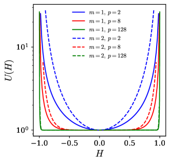
Figure 2: Confinement potential Eq. (18). At small $H$, the potential can be varied from a harmonic profile for $p=2$ to a square potential for larger $p$. Close to the walls, the divergence of the potential is controlled by $m$.

The force on the membrane along the $Z$ direction is normalized as $F_{Z}=(h_{0}/\mathcal{U}_{0})f_{z}$. In normalized coordinates, $L_{X}$ (resp. $L_{Y}$) represents the length of the system in the $X$ (resp. $Y$) direction in normalized variables.

For a given confinement potential, the dynamics is controlled by two dimensionless parameters: the normalized density of excess area

$$\Delta A_{*}=\frac{1}{\epsilon^{2}}\,\frac{\Delta\mathcal{A}}{\mathcal{L}_{x}\mathcal{L}_{y}}=\frac{\Delta A}{L_{X}L_{Y}}$$ (19)

and the normalized shear velocity $V$.

We also define the normalized forces on each wall as

$$F_{wX} =\frac{24\kappa^{1/4}h_{0}^{1/2}}{\mathcal{U}_{0}^{5/4}}f_{wx}=\bar{\nu}V+12\langle H\partial_{X}HF_{Z}\rangle,$$

$$F_{wY} =\frac{24\kappa^{1/4}h_{0}^{1/2}}{\mathcal{U}_{0}^{5/4}}f_{wy}=12\langle H\partial_{Y}HF_{Z}\rangle,$$ (20)

and we have introduced the spatial averaging notation for any function $\psi$

$$\langle\psi\rangle=\frac{1}{L_{X}L_{Y}}\int_{0}^{L_{X}}dX\int_{0}^{L_{Y}}dY\psi.$$ (21)

Thus, the two contributions of the membrane to the tangential forces on each wall read

$$F_{\mathrm{mem},X}=12\langle H\partial_{X}HF_{Z}\rangle,\quad F_{\mathrm{mem},Y}=12\langle H\partial_{Y}HF_{Z}\rangle.$$ (22)

III Dynamics of confined membranes without shear

III.1 Frozen labyrinthine states

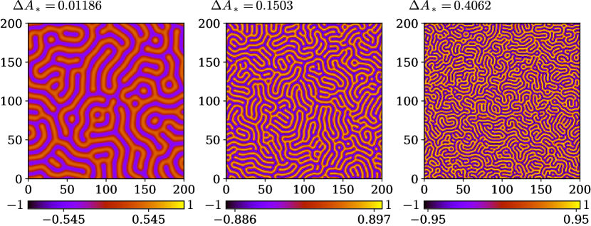
Figure 3: Labyrinthine patterns in quiescent conditions. Top-views of the membrane height in steady state for several membrane excess areas in quiescent conditions ($V=0$). The marks on the color bars show the minimum and maximum membrane heights in each image.

In the absence of shear $V=0$ and starting from random initial conditions the membrane dynamics relaxes quickly to a frozen isotropic labyrinthine pattern. In this regime, the tension is always negative, as expected for a membrane in compression due to confinement with a fixed excess area. We use a numerical scheme described in Ref.To et al. (2018) which preserves precisely the membrane area, and random initial conditions as described in Appendix C. Fig. 3 shows topviews of the membrane height profile for several membrane excess area. The minimum and maximum membrane height are shown as marks on the color bars. A visual inspection of the topviews shows that the wrinkle wavelength $\lambda$ decreases and the maximum membrane height $\lvert h\rvert_{\mathrm{max}}$ increases as the excess area $\Delta A_{*}$ is increased. Simulation movies for $V=0$ are shown in Electronic Supplementary Information (ESI)†(Movie 1).

III.2 Sine-ansatz

In the absence of shear, the last term of Eq. (2) vanishes, and our model shares similarities with previous models described in the literature, which leads to the formation of wrinkles. For example, the model for wrinkle formation in stressed films on soft substrates reported in Ref.Huang and Im (2006), initially presents some amount of coarsening, where the wavelength of the wrinkles increases with time, and ultimately leads to a frozen labyrinthine pattern of wrinkles in the presence of equiaxial stress. Labyrinthine patterns have also been reported in the literature for the Swift-Hohenberg equation by Le Berre et al. Le Berre et al. (2002). However, our equations differ from these models and exhibit two main specific features. First, our non-local tension is constant in space and depends on time via Eq. (4), while it is a local tensorial stress in Ref.Huang and Im (2006), and a time-independent constant in the Swift-Hohenberg equation. Second, our confinement potential is different and diverges at the walls.

We have also recently reported on the observation of labyrinthine patterns or endless coarsening in the dynamics of lipid membranes subject to a double-well adhesion potential  To et al. (2018). Following the same lines as in our previous study To et al. (2018), we relate the wrinkle wavelength $\lambda$ and $\Delta A_{*}$ analytically using an ansatz that assumes a sinusoidal membrane profile

$$H(\zeta)=a\cos(q\zeta),$$ (23)

where $a$ and $q$ are two positive constants, and $\zeta$ is the space variable locally orthogonal to the wrinkle orientation in the $X,Y$ plane. Such a sinusoidal membrane profile can be seen in Fig. 1(b). The red curve shows a cross section of the membrane profile by a vertical plane. We see that a part of the curve on the right is almost periodic and sinusoidal. In this part, the cross section direction is almost perpendicular to the direction of the membrane wrinkles. In the other parts of the curve, where the cross section is not perpendicular to the direction of the wrinkles, the membrane profile looks more random, sometimes with flatter parts when the section is aligned with the top of the crests, or the bottom of the valleys of the wrinkles. Substitution of Eq. (23) into Eq. (4) leads to a simple relation between $q$ and $\Delta A_{*}$

$$\Delta A_{*}=\frac{1}{4}q^{2}a^{2}=\frac{\pi^{2}}{\lambda^{2}}a^{2},$$ (24)

where $\lambda=2\pi/q$ is the wrinkle wavelength. This geometrical relation was already reported in previous workCerda and Mahadevan (2003); To et al. (2018). Within the sine ansatz the root-mean-square corrugation of the membrane height $\langle H^{2}\rangle$ is proportional to the amplitude $\langle H^{2}\rangle^{\frac{1}{2}}=a/\sqrt{2}$.

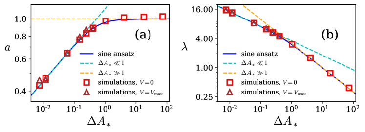
Figure 4: Sine-ansatz predictions of wrinkle size. (a) Wrinkle amplitude $a$ and (b) wrinkle wavelength $\lambda$ are plotted as a functions of the membrane excess area $\Delta A_{*}$. Blue solid curves: full analytical results from the sine ansatz (see Appendix B). Cyan dashed lines: analytical results in limit of small $\Delta A_{*}$ in Eq. (25), leading to $\lambda\simeq 3.5765\Delta A_{*}^{-\frac{3}{10}}$, $a\simeq 1.1385\Delta A_{*}^{\frac{1}{5}}$ for $m=1$ and $p=8$. Yellow dashed lines: analytical results in limit of large $\Delta A_{*}$: $a=1$ and $\lambda=\pi\Delta A_{*}^{-1/2}$. Red squares: simulation results for $V=0$. Brown triangles: simulation results for periodic state under shear at $V=V_{\mathrm{max}}$.

A second relation between $q$ and $a$ is obtained from the minimization of the total energy, including bending rigidity and interaction potential, for a fixed excess area. Below, we report on the limit of small and large excess area. The details of the general calculation are reported in Appendix B.

In the limit of small excess areas $\Delta A_{*}\ll 1$, the result takes a simple form

$$\lambda=\pi C_{m,p}\,\Delta A_{*}^{-\frac{1}{2}+\frac{2}{p+2}},\quad\quad a=C_{m,p}\,\Delta A_{*}^{\frac{2}{p+2}},$$ (25)

where the expression of the constant $C_{m,p}$ is given in Eq. (98). In this small amplitude regime, two limiting cases are in order. First, when $p=2$ (shown as blue curves in Fig. 2), the potential is harmonic for small $h$ and the wavelength $\lambda$ is independent of $\Delta A_{*}$. This means that the wrinkle lengthscale is identical to the scaling lengthscale $\ell_{\parallel}$. In addition, we have $a\sim\Delta A_{*}^{1/2}$. Second, the opposite case of large $p\gg 1$ corresponds to a square-like potential which is very flat between the two walls (shown as green curves in Fig. 2). In this square-like potential, $\lambda\rightarrow\pi\Delta A_{*}^{-1/2}$ and the amplitude $a\rightarrow 1$ is independent of $\Delta A_{*}$. Hence, the excess area is stored by an increase of amplitude at fixed wavelength when $p=2$, and by a decrease of wavelength at fixed amplitude when $p\gg 1$.

For large excess area $\Delta A_{*}\gg 1$, the membrane amplitude approaches the walls so that $a\approx 1$. In this case, the sine ansatz in Eq. (24) implies that the wavelength $\lambda$ is independent of $m$ and $p$,

$$\lambda=\pi\Delta A_{*}^{-\frac{1}{2}},\quad\quad a=1.$$ (26)

Interestingly, we notice the small excess area expansion for large $p\gg 1$ catches quantitatively the limit of large excess area.

The predictions of the sine-ansatz and the related small and large excess area limits for the potential Eq. (18) with $m=1,p=8$ are in quantitative agreement with the full simulations, as shown in Fig. 4. Note that the sine anstaz discards the meandering and branching of wrinkles in labyrinthine patterns. The accuracy of the prediction of the sine ansatz therefore indicates that meandering and branching play a negligible role in the section of the wavelength.

IV Dynamics of confined membrane under shear: simulation results

In this Section we present the simulation results in the presence of shear, when $V\neq 0$. All simulations are started with random initial conditions.

IV.1 Steady-drifting states and Oscillatory states

In most simulations, and independently from the value of the shear rate $V$, the membrane reaches a constant profile at long times which drifts with a constant velocity $\mathbf{V}_{d}$ with non-vanishing components $V_{dX}$ and $V_{dY}$ along $X$ and $Y$. Some steady-state configurations together with the direction of their drifts in the $X$ direction are shown in Fig. 5. Simulation movies for $V_{dX}>0$, $V_{dX}<0$ and $V_{dX}\approx 0$ are shown in ESI†(Movie 2, Movie 3 and Movie 4, respectively). The method for the measurements of the drift velocities, and a table summarizing their values are reported in Appendix D. In addition, as in the quiescent case, the tension is always negative.

Since the dynamical equation (2) is invariant under the variable changes $Y\rightarrow-Y$, and $(X,H)\rightarrow(-X,-H)$, there is no preferred drift direction. The drift can therefore be seen as a consequence of the random asymmetry of the disordered steady-states. More precisely, drifting steady-state profiles obey

$$-V_{dX}\partial_{X}H-V_{dY}\partial_{Y}H=-\Delta^{2}H+\Sigma_{0}\Delta H-U^{\prime}(H)-VH\partial_{X}H.$$ (27)

Hence, for each steady-state $H(X,Y)$ with drift velocity $(V_{dX},V_{dY})$, there is a second steady-state $H(X,-Y)$ with drift velocity $(V_{dX},-V_{dY})$, and a third steady-state $-H(-X,Y)$ with drift velocity $(-V_{dX},V_{dY})$. As a consequence, although a non-zero drift can be present in a given simulation, the drift averaged over many simulations started with random initial conditions should vanish. Indeed we observe in the simulations that the signs of $V_{dX}$ and $V_{dY}$ can be positive and negative with roughly equal probabilities.

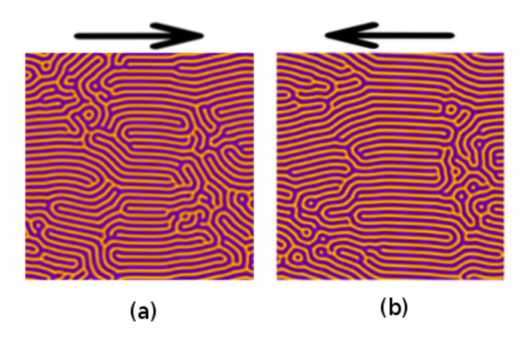
Figure 5: Drift direction. Membrane profiles for $\Delta A_{*}=0.1503$ and $V=2$ and different initial conditions with opposite drifting directions along $X$ to the right (a) and to the left (b).

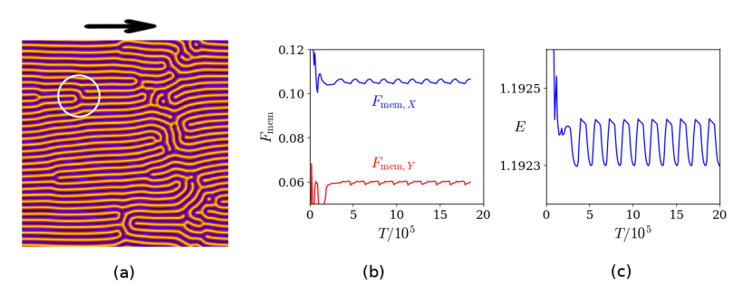
Figure 6: Oscillations. (a) Membrane pattern drifting to the right with an oscillating pair of defects (indicated by the white circle) for $\Delta A_{*}=0.1503$ and $V=3$. (b) Corresponding components of the membrane force acting on each wall $F_{\mathrm{mem}}$ . (c) Evolution of the corresponding membrane energy $E$ from Eq. (28).

Note that, although the final state is a steady-drifting state in the vast majority of cases, this is not always the case. Indeed, for some values of $\Delta A_{*}$ and $V$ we found patterns that oscillate periodically. As an example we show the membrane profile for $\Delta A_{*}=0.1503$ and $V=3$ in Fig. 6(a). In this simulation, there is a pair of defects (shown by the white circle) that moves alternately forwards and backwards along the shear direction $x$. We define a defect as the end of the line following the top of a wrinkle crest or the bottom of a wrinkle valley (more example of defects will be provided below in Fig. 8). This oscillation is superimposed to a global drift. Simulation movie related to this case is shown in ESI†(Movie 5).

The existence of drifting or oscillatory states can be related to the non-variational character of the shear term $VH\partial_{X}H$ in Eq. (15). Indeed, as discussed in Ref.To et al. (2018), in the absence of this term, the dynamics is decreasing the free energy of the membrane, comprising bending energy and potential energy

$$E=\left\langle\frac{1}{2}(\Delta H)^{2}+U(H)\right\rangle.$$ (28)

Hence, $\partial_{T}E<0$ when $\partial_{T}H\neq 0$. Such monotonic decrease of the energy implies that the system cannot evolve and go back to the same state, which would correspond to the same energy: drift and oscillations are forbidden. This strong constraint is lost in the presence of non vanishing shear.

The time evolution of the energy $E$ for some drifting steady-states in Fig. 7 shows that in some cases the membrane energy can increase with time when $V\neq 0$. In addition, while the energy $E$ ultimately reaches a constant value in drifting steady-state as shown in Fig. 7, it oscillates in the periodic oscillating-drifting state as shown in Fig. 6(c).

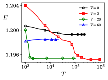
Figure 7: Evolution of the membrane energy $E$ with time $T$ when the final state is a steady-state with a constant drift. All simulations are performed at $\Delta A_{*}=0.1503$.

IV.2 Dynamical regimes as a function of the shear rate $V$

The dependence of the membrane patterns on the shear velocity $V$ exhibits 4 different regimes. Typical configuration corresponding to these regimes are presented in the top panels in Fig. 8.

Regime I. At small shear velocities, the membrane presents an isotropic labyrinthine pattern which is very similar to the pattern found in the absence of shear. This isotropy is clearly seen in the Fourier transform on the first panel in Fig. 8. This pattern also exhibits the same wavelength as in the absence of shear, as shown in Fig. 4(b). The pattern exhibits a random drift which increases in amplitude when $V$ increases. The dift is also anisotropic, with a larger amplitude along the $X$ axis, i.e. $|V_{dX}|>|V_{dY}|$.

Regime II. When the shear rate $V$ exceeds a critical value $V_{c}$, the membrane starts to reorganize and becomes anisotropic, with wrinkles partially aligned in the $X$ direction. The Fourier transform in the second figure on the top right of Fig. 8 presents a clear anisotropy. This is the only regime where oscillatory states have been observed.

Regime III. For larger shear rates $V>V_{p}$, the membranes form a parallel array of wrinkles with dislocations. There are 4 types of dislocations, which can be deduced from each other via the $X\rightarrow-X$, and the $H\rightarrow-H$ symmetries. In this regime, the density of dislocations increases with increasing excess area $\Delta A_{*}$. We also observe that dislocations are mostly found in pairs. Within each pair, one dislocation can be deduced from the other by the symmetry $H(X,Y)\rightarrow-H(X,Y)$. In addition, the number of wrinkles passing between the two dislocations varies from one pair to the other.

Regime IV. For large shear velocity $V\geq V_{\mathrm{max}}$, dislocations disappear and the membrane exhibits a perfect array of parallel stripes. Some simulation movies for this case are shown in ESI†(Movie 6). The final wavelength in this state, reported in Fig. 4(b) with brown triangles , is again in very good agreement with the wavelength of the frozen state without shear and with the sine ansatz.

Finally, note that, due to slowness in the numerical convergence for large $\Delta A_{*}$ and large $V$, we have only explored systematically the cases $\Delta A_{*}<1$. The few simulations performed with larger $\Delta A_{*}$ suggest a similar scenario. Movies of these cases are reported in ESI†(Movie 7).

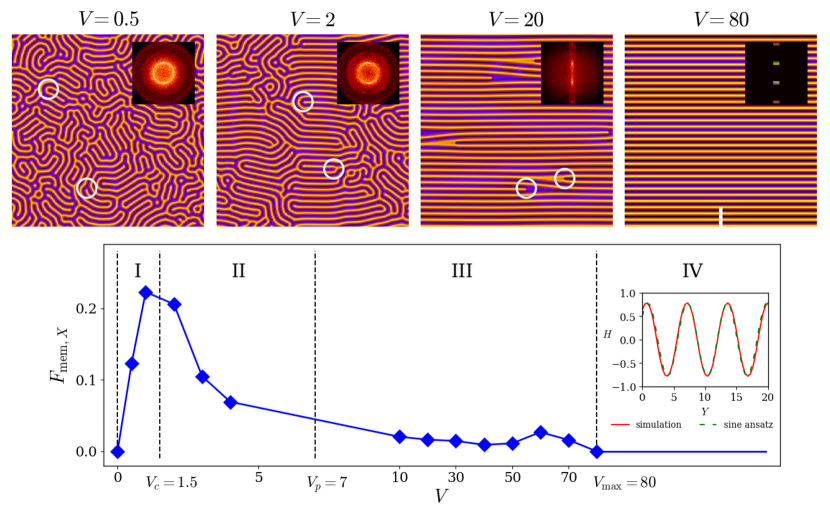
Figure 8: Steady-state regimes of confined membranes under shear, and related tangential forces on the walls. All simulation profiles and forces are obtained for $\Delta A_{*}=0.1503$. Top panels: The membrane profile exhibits four different regimes as the shear velocity is varied $V$ in simulations. White circles highlight some representative defects. Insets (top panels): zooms of the Fourier transforms in log scale with $\lvert q_{x}\rvert<2\pi/5$ and $\lvert q_{y}\rvert<2\pi/5$; for $V=80$, $\lvert q_{x}\rvert<\pi/50$. Bottom panel: variation of the membrane force along $X$ on each wall $F_{\mathrm{mem},X}$ as the function of the shear rate $V$. In order to show Regimes I and II, the interval from $V=0$ to $V=10$ is magnified in the abscissa. Inset (bottom panel): cross-section of the membrane profile in Regime IV from simulation along the white vertical line of the top view at $V=80$. The profile is very close to the prediction of the sinusoidal ansatz Eq. (23,25). The same regimes, with similar membrane profiles and similar variations of the force, are observed for different values of $\Delta A_{*}$, as shown in Fig. 9.

IV.3 Forces on the walls as a function of the shear rate $V$

The 4 dynamical regimes of the membrane give rise to distinctive behaviours of the tangential forces acting on the walls. The dependence of $F_{\mathrm{mem},X}$ on $V$ is summarized in the schematic at the bottom figure of Fig. 8. In Fig. 9, the forces measured in simulations are plotted as function of $V$ for different $\Delta A_{*}$.

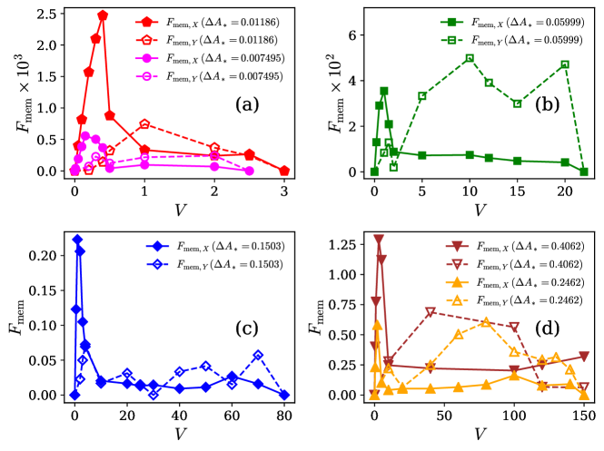
Figure 9: Membrane contribution to the tangential forces on each wall in steady state. $F_{\mathrm{mem}}$ is plotted as a function of the shear rate $V$ for different excess areas $\Delta A_{*}$. Continuous lines: $F_{\mathrm{mem},X}$. Dashed lines: $F_{\mathrm{mem},Y}$. The membrane excess area $\Delta A_{*}$ increases from Fig. (a) to (d).

In Regime I, the force $F_{\mathrm{mem},X}$ increases linearly with the shear velocity $V$. The force $F_{\mathrm{mem},Y}$ is very small and can exhibit both signs.

When the shear rate is increased further, the force increases slower than linearly and at the critical shear rate $V_{c}$ the force reaches a peak. The value of $V_{c}$ as a function of the excess area $\Delta A_{*}$ is reported in Fig. 10. By convention, and although some weak reorganisation of the membrane pattern can be observed just before the peak, we use $V>V_{c}$ as a formal definition of Regime II. In Regime II, the steady-state force along $X$ drops quickly as $V$ increases. When the dynamics is oscillatory, the forces along the $X$ and $Y$ directions are oscillatory, as shown in Fig. 6(b).

As the shear rate is increased further, the membrane reaches Regime III dominated by dislocations where the force along $X$ presents a noisy plateau. Simultaneously, the force along $Y$ becomes very large in amplitude, but still with equal probability in the $+Y$ and $-Y$ directions.

Finally, in regime IV, as $V\geq V_{\mathrm{max}}$, the force vanishes in both directions. The value of $V_{\mathrm{max}}$ as a function of the excess area is reported in Fig. 10.

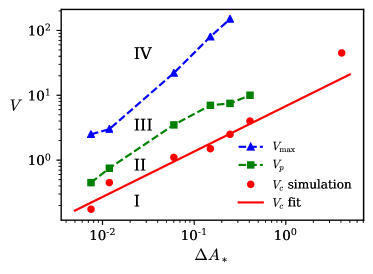
Figure 10: Non-equilibrium phase diagram with four different regimes. These regimes correspond to those reported in Fig. 8 and 9. The three critical velocities $V_{c}$, $V_{p}$, and $V_{\mathrm{max}}$ are defined in the text. The red solid line reports the fit $V_{c}=6.7941\Delta A_{*}^{\frac{7}{10}}$ with the predicted exponent for $\Delta A_{*}\ll 1$, see Eq. (30). Dashed lines are guide to the eye.

V Critical shear rate $V_{c}$

In this section, we obtain an estimate of the critical shear rate $V_{c}$ from a simple balance between different terms in Eq. (15). In order to do so, we compare the shear term $VH\partial_{x}H$ and terms associated to the force $F_{Z}$. In the spirit of the sine-ansatz where the amplitude $a$ and wavelength $\lambda$ of the pattern result from the minimization of the energy, the three terms in the force, associated to bending rigidity, tension and confining potential, have similar magnitudes. We therefore choose arbitrarily to compare the shear term with the bending rigidity term, i.e. we assume that $V_{c}$ is such that $VH\partial_{X}H\sim\Delta^{2}H$.

Assuming the sine-profile ansatz following the same lines as in the analyis of the dynamics of the membrane without shear discussed above, we set $H=a\cos(q\zeta)$ where $a$ is the amplitude, $q$ is the wave number and $\zeta$ is the space variable orthogonal to the wrinkles in the $X,Y$ plane. Each derivative brings a prefactor $q$ and we obtain $C_{0}q^{4}a=V_{c}qa^{2}$, where $C_{0}$ is a number of the order of one. This relation is re-written as

$$V_{c}=C_{0}\frac{q^{3}}{a}.$$ (29)

Since the membrane profile at small shear rates is not affected by shear as observed in the simulations, we assume that $a$ and $q$ obey the same laws as in the case without shear. Thus, in the limit of small excess area, we use Eq. (25), and obtain

$$V_{c}=8C_{0}C_{m,p}^{-4}\Delta A_{*}^{\frac{3}{2}-\frac{8}{p+2}}.$$ (30)

Such a power-law behavior with $C_{0}\approx 1.43$ is in good agreement with simulations at small $\Delta A_{*}$, as shown in Fig. 10.

In the limit of large excess area, the same procedure (combining Eq. (26) with Eq. (29)) leads to

$$V_{c}=8C_{0}\Delta A_{*}^{3/2},$$ (31)

with a possibly different value of $C_{0}$ from that of the regime at small excess area. We could not obtain accurate simulations at large large $\Delta A_{*}$ and large $V$, and we can therefore not extract the value of $C_{0}$ for large $\Delta A_{*}$. However, we have obtained $V_{c}\approx 45$ for $\Delta A_{*}=4.07$, which suggests $C_{0}\approx 0.7$ from Eq. (31).

VI Forces in drifting steady-states

In a drifting steady-states we can combine Eqs. (22) and (27) to obtain useful expressions of the force exerted by the membrane on each wall

$$F_{\mathrm{mem},X}=12\left[V\langle(H\partial_{X}H)^{2}\rangle-V_{dX}\langle H(\partial_{X}H)^{2}\rangle-V_{dY}\langle H\partial_{X}H\partial_{Y}H\rangle\right],$$

$$F_{\mathrm{mem},Y}=12\left[V\langle H^{2}\partial_{X}H\partial_{Y}H\rangle-V_{dX}\langle H\partial_{X}H\partial_{Y}H\rangle-V_{dY}\langle H(\partial_{Y}H)^{2}\rangle\right].$$ (32)

As discussed in the following, these expressions allow one to study the forces on the basis of the analysis of the membrane profile.

VI.1 Small shear rates

For small shear rates in Regime I, the configuration of the membrane is similar to that obtained in the absence of shear. Since the configuration without shear is disordered and isotropic, the asymmetry of the membrane configuration which breaks the $X\rightarrow-X$ or the $Y\rightarrow-Y$ symmetries in a large system is small and random. As a consequence, the drift velocities $V_{dX}$ and $V_{dY}$ are also small and random. Hence, the contributions proportional to these velocities in Eqs. (VI) are negligible as compared to the first term proportional to $V$ which does not vanish for symmetric and isotropic configurations.

Therefore, to leading order, the membrane contribution to the force is then given by

$$F_{\mathrm{mem},X}=12V\langle(H\partial_{X}H)^{2}\rangle.$$ (33)

The spatially averaged quantity $\langle(H\partial_{X}H)^{2}\rangle$ is evaluated using the sine-profile ansatz. Since the labyrinthine pattern is isotropic, we average over all possible orientations of the wrinkles. We therefore define the angle $\theta$ between the wrinkle orientation and the $Y$ axis. In the sine ansatz Eq. (23), the coordinate orthogonal to the wrinkle then reads $\zeta=X\cos\theta+Y\sin\theta$. The average takes the form

$$\langle(H\partial_{X}H)^{2}\rangle=\frac{1}{2\pi}\int_{0}^{2\pi}d\theta\frac{1}{\lambda}\int_{0}^{\lambda}d\zeta(H\partial_{X}H)^{2},$$ (34)

where $H=a\cos(q\zeta)$ and $\partial_{X}H=-aq\cos\theta\sin(q\zeta)$. Performing the integration on $\zeta$ and $\theta$, we obtain

$$\langle(H\partial_{X}H)^{2}\rangle=\frac{a^{4}q^{2}}{16}.$$ (35)

Since the labyrinthine pattern is not affected by shear for small $V$, we substitute the expressions of $a$ and $q$ that are obtained from the energy minimization of the sine-ansatz without shear in Eq. (35). Thus, in regime I, i.e., for small $V$ we obtain from Eq. (33)

$$F_{\mathrm{mem},X}=\frac{3}{4}Va^{4}q^{2}.$$ (36)

In the limit of small $\Delta A_{*}$, this leads to

$$F_{\mathrm{mem},X}=3C_{m,p}^{2}V\Delta A_{*}^{1+\frac{4}{p+2}},$$ (37)

where $C_{m,p}$ is given in Eq. (98). This expression is in quantitative agreement with the simulation results, as shown in Fig. 11. In the limit of large excess area, we obtain

$$F_{\mathrm{mem},X}=3V\Delta A_{*}.$$ (38)

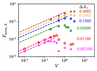
Figure 11: Regime I: linear behavior of the membrane force at small shear rates. $F_{\mathrm{mem},X}$ in steady state is plotted as a function of the shear rate $V$ for different $\Delta A_{*}$. The dashed lines are the linear behavior predicted by Eq. (37). Symbols: simulation results. The membrane excess area $\Delta A_{*}$ increases from the bottom curve to the top curve.

VI.2 Large shear rates: defect dependent membrane forces

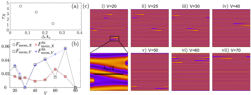
Figure 12: Regime III: dislocation-dominated forces. (a) Evolution of $\tau_{x}$ from Eq. (42) with excess area $\Delta A_{*}$. (b) The black solid line with $\bigcirc$ (resp. $\Box$) represents the membrane force $F_{\mathrm{mem},X}$ (resp. $F_{\mathrm{mem},Y}$) obtained in simulations for $\Delta A_{*}=0.1503$ and evaluated from Eqs. (22). The red dotted line with $\times$ is a multiple linear regression of $F_{\mathrm{mem},X}$ for $V\geq 20$ using Eq. (51) ($a_{\mathrm{wr,X}}\approx 32.4$ and $a_{\mathrm{dis,X}}\approx 8.6$). The blue dotted line with $+$ is a linear regression of $F_{\mathrm{mem},Y}$ using Eq. (52) ($a_{\mathrm{wr,Y}}=35.4$, the simulations $V=30$ and $V=60$ have been removed for linear regression, see text). (c) Membrane profile in steady-states corresponding to the points in panel (b). Values of $(n,N,n_{0})$ (see text for definition) extracted from the images for various shear rates: i): $V=20$ (4,3,2), ii): $V=25$ (3,2,1), iii): $V=30$ (2,2,0) iv): $V=40$ (1,1,1), v): $V=50$ (1,1,1), vi): $V=60$ (1,2,1) and vii): $V=70$ (1,1,1). The zoom shows that a half-wavelength $\lambda_{X}/2$ in the tilted wrinkles zone corresponds approximately to the distance between the two dislocation cores in a pair.

For large shear rates in regime III, the configuration of the membrane is composed of a few dislocations on a set of almost parallel stripes aligned along $X$. Thus, the configuration is globally anisotropic. The background of parallel wrinkles along $X$ provides no contribution to the force exerted by the membrane on the walls from Eqs. (VI). The dislocation pairs therefore can be seen as elementary building blocks, each pair providing its own contribution to the total force.

A close inspection of the images of the membrane in Fig. 12 indicates that for each pair of dislocations, tilted wrinkles pass between the two dislocations. Each wrinkle is approximately shifted by one period along $Y$ when passing between the two dislocation of a dislocation pair. We therefore design a simple approximation where all the wrinkles passing between the pairs are straight and identical, and are tilted only in a zone of length $\lambda_{X}$ along $X$. This leads to the sine-profile ansatz

$$H=a\cos\left(\vartheta q_{X}X+q_{Y}Y\right),$$ (39)

with $\vartheta=1$ or $-1$ when the wrinkle slope is negative or positive respectively, $q_{X}=2\pi/\lambda_{X}$ where $\lambda_{X}$ is the wavelength of tilted wrinkles along $X$-axis or shear direction (see Fig. 12). The quantities $q_{Y}$ and $\lambda_{Y}$ are defined in a similar fashion.

The membrane contributions to the force Eq. (VI) is integrated over the size $\lambda_{X}$ of the tilted zone along $X$. In order to isolate the contribution of each tilted wrinkle, we also integrate over a single period $\lambda_{y}$ along $Y$. Using the ansatz in Eq. (39), the contributions proportional to $V_{dX}$ and $V_{dY}$ vanish, and we find that one single period of tilted wrinkle along $X$ and along $Y$ exerts the forces

$$F_{\mathrm{mem},X}^{\mathrm{wr}}=\frac{1}{L_{X}L_{Y}}6\pi^{2}V\frac{\lambda_{Y}}{\lambda_{X}}a^{4},$$ (40)

$$F_{\mathrm{mem},Y}^{\mathrm{wr}}=\frac{1}{L_{X}L_{Y}}6\pi^{2}Va^{4}\vartheta.$$ (41)

Moreover, simulations in regime III are consistent with a linear increase of $\lambda_{X}$ with the shear rate:

$$\lambda_{X}=\tau_{X}V$$ (42)

with $\tau_{X}$ a constant. A measurement of $\lambda_{X}$ based on the distance between two successive zeros of the membrane profile in the tilted region allows one to estimate $\tau_{X}$ by linear regression. The value of $\tau_{X}$ as a function of $\Delta A_{*}$ is reported in Fig. 12 (a). In addition, since the angle of the wrinkles with the $X$ direction is small, we simply assume that $\lambda_{Y}\simeq\lambda$. Combining these assumptions for $\lambda_{X}$ and $\lambda_{Y}$ Eq. (40) is written as

$$F_{\mathrm{mem},X}^{\mathrm{wr}}=\frac{1}{L_{X}L_{Y}}12\pi^{3}V\frac{a^{4}}{q\tau_{X}}.$$ (43)

In addition to the contribution of the tilted wrinkles, there is also a contribution to the force caused by the cores of the dislocations. As discussed above, the second dislocation in a pair is obtained by a symmetry $H(X,Y)\rightarrow-H(-X,Y)$ from the first one. Moreover an analysis of the simulation images reveals the approximate symmetry of each dislocation core under the transformation $Y\rightarrow-Y$. Using these symmetry properties and Eqs. (VI), we obtain the contributions for one pair of dislocation cores

$$F_{\mathrm{mem},X}^{\mathrm{disloc,pair}}=24V\langle(H\partial_{X}H)^{2}\rangle_{core},\quad F_{\mathrm{mem},Y}^{\mathrm{disloc,pair}}=0,$$ (44)

where $\langle(H\partial_{X}H)^{2}\rangle_{core}$ is evaluated by means of integration around one single dislocation core

$$\langle(H\partial_{X}H)^{2}\rangle_{core}=\frac{1}{L_{X}L_{Y}}\int_{core}dX\int_{core}dY(H\partial_{X}H)^{2}.$$ (45)

Assuming that the profile of the dislocation core does not depend on $V$, the contributions to the membrane forces take the form

$$F_{\mathrm{mem},X}^{\mathrm{wr}}=\frac{a_{\mathrm{wr},X}}{L_{X}L_{Y}},\quad F_{\mathrm{mem},Y}^{\mathrm{wr}}=\vartheta\frac{a_{\mathrm{wr},Y}}{L_{X}L_{Y}}V,\quad F_{\mathrm{mem},X}^{\mathrm{disloc,pair}}=\frac{a_{\mathrm{dis},X}}{L_{X}L_{Y}}V,$$ (46)

where $a_{\mathrm{wr},X}$, $a_{\mathrm{wr},Y}$ and $a_{\mathrm{dis},X}$ are constants independent of $V$, $L_{X}$, $L_{Y}$, and $\vartheta$

$$a_{\mathrm{wr},X}=12\pi^{3}\frac{a^{4}}{\tau_{X}q},$$ (47)

$$a_{\mathrm{wr},Y}=6\pi^{2}a^{4}.$$ (48)

The third constant, which accounts for the contribution of the dislocation core is unknown

$$a_{\mathrm{dis},X}=24\int_{core}dX\int_{core}dY(H\partial_{X}H)^{2}.$$ (49)

Summing the contributions of all dislocation pairs in the system, the total force exerted on each wall can be written as

$$F_{\mathrm{mem},X}=\frac{n}{L_{X}L_{Y}}F_{\mathrm{mem},X}^{\mathrm{wr}}+\frac{N}{L_{X}L_{Y}}F_{\mathrm{mem},X}^{\mathrm{disloc,pair}},$$

$$F_{\mathrm{mem},Y}=\frac{n_{0}}{L_{X}L_{Y}}|F_{\mathrm{mem},Y}^{\mathrm{wr}}|,$$ (50)

where $n$ is the total number of wrinkles within pairs of dislocations, $n_{0}$ is the number of wrinkles with negative slope minus the number of wrinkles with positive slope and $N$ is the total number of pairs of dislocations. The total forces Eqs. (VI.2) may be rewritten as

$$F_{\mathrm{mem},X}=a_{\mathrm{wr},X}\frac{n}{L_{X}L_{Y}}+a_{\mathrm{dis},X}\frac{N}{L_{X}L_{Y}}V,$$ (51)

$$F_{\mathrm{mem},Y}=a_{\mathrm{wr},Y}\frac{n_{0}}{L_{X}L_{Y}}V.$$ (52)

As seen from Fig. 12 (b), the Eqs. (51,52) provides an excellent fit to the simulation results. For $\Delta A_{*}=0.1503$ a linear regression leads to $a_{\mathrm{wr},X}^{\mathrm{fit}}\approx 32.4$, $a_{\mathrm{dis},X}^{\mathrm{fit}}\approx 8.6$ and $a_{\mathrm{wr},Y}^{\mathrm{fit}}\approx 35.4$.

However, two remarks are in order. First, the fit fails to describe the rare cases when two dislocation pairs are very close to each other. This is for example the case in Fig. 12 (b) and (c)(vi) for $V=60$. Second, the analytical expressions of the constants Eqs. (47,48) provide the correct order of magnitude but are not quantitatively accurate. Indeed, using the expressions of $a$ and $q$ from the sine ansatz in the limit of small excess area Eq. (25), they lead to $a_{\mathrm{wr},X}\approx 41.6$ and $a_{\mathrm{wr},Y}\approx 21.6$ for $\Delta A_{*}=0.1503$. These discrepancies could originate in the crudeness of the assumptions leading to Eqs. (47,48), such as straight tilted wrinkles, and the absence of smooth decay of the perturbation away from the dislocation pair. Despite the difficulty in finding an accurate analytical expression for the prefactors $a_{wr}$ in Eqs. (51,52), the simple dependence of the forces on the topological numbers $n$, $N$ and $n_{0}$ is remarkable.

Since the asymmetry of the membrane profile in steady-state emerges from the randomness of initial conditions, we expect that $n_{0}/n\rightarrow 0$ and $n_{0}/N\rightarrow 0$ as $L_{X},L_{Y}\rightarrow\infty$, in the limit of large systems. Therefore, the dominant contribution to the force would be along $X$. However, our simulations are performed in a finite simulation box and the number of dislocations usually does not exceed 10. Hence at large shear rates when the terms proportional to $V$ dominate, since the prefactor of the force due to tilted wrinkles is larger in the $Y$ direction $a_{\mathrm{wr},Y}>a_{\mathrm{dis},X}$, we often observe that $F_{\mathrm{mem},Y}=a_{\mathrm{wr},Y}n_{0}V>F_{\mathrm{mem},X}\approx a_{\mathrm{dis},X}NV$ although $n_{0}\leq N$. However, the forces along $X$ should dominate in the limit of very large systems where we expect $N\gg n_{0}$.

VII Critical shear rate $V_{\mathrm{max}}$

The transition to regime IV, where all dislocations disappear leading to a perfect array of parallel wrinkles along $X$, occurs at large shear rates. Here, we present evidences that this transition could originate in a finite size effect.

Indeed, when the shear rate is very large, the distance between the dislocations within a pair increases (see Eq. (42)) and becomes comparable to the system size. The distance between two dislocation cores within a pair is roughly equal to $\lambda_{X}/2$, as seen from the zoom in Fig. 12(c). Due to the periodic boundary conditions in the $X$ direction, the complementary distance between the two dislocations is $L_{X}-\lambda/2$. The transition roughly occurs when these two distances are similar $\lambda_{X}/2\approx L_{X}-\lambda_{X}/2$, i.e., when $\lambda_{X}\approx L_{X}$. Using Eq. (42), this criterion leads to $\tau_{X}V/L_{X}\approx 1$.

In Fig. 13, we show the ratio $\tau_{X}V/L_{X}$ for three values of $\tau_{X}$ that have been extracted from simulations in Regime III (see Fig. 12(a)). Fluctuations are large in Fig. 13 due to poor statistics with few simulations and few dislocations in each simulation. However, the ratio $\tau_{X}V/L_{X}$ is around one in all cases, and these results therefore support the hypothesis of a transition to regime IV controlled by finite size effects.

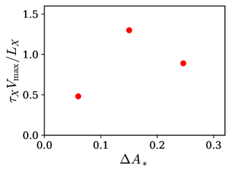
Figure 13: Finite size effects in the transition to Regme IV. The ratio $\tau_{X}V_{\mathrm{max}}/L_{X}$ is plotted for three excess areas $\Delta A_{*}$ with $L_{X}=200$. The values of $\tau_{X}$ are from Fig. 12(a).

VIII Summary and Discussions

VIII.1 Summary of results

In summary, we have studied the dynamics of a lipid membrane confined between two flat walls in the presence and in the absence of shear. We have also evaluated the tangential forces exerted by the membrane on each wall due to its complex nonlinear dynamics in the presence of shear. In this section, we provide a concise recapitulation of the main results.

In the absence of shear, the membrane forms a disordered labyrinthine pattern of wrinkles. The wavelength and amplitude of the pattern are described quantitatively using a sine-ansatz. The results depend on the free energy potential that confines the membrane between the walls. We have used the confinement potential

$${\cal U}(h)=\frac{{\cal U}_{0}}{[1-(h/h_{0})^{p}]^{m}}.$$ (53)

Two different regimes are identified, depending on the normalized excess area

$$\Delta A_{*}=\frac{\Delta{\cal A}}{{\cal L}_{x}{\cal L}_{y}}\,\frac{\ell_{\parallel}^{2}}{h_{0}^{2}},$$ (54)

where $\ell_{\parallel}$ is defined in Eq. (11). In physical units, we have

$$\lambda =\pi\ell_{\parallel}\times\left\{\begin{array}[]{ll}C_{m,p}\Delta A_{*}^{-\frac{1}{2}+\frac{2}{p+2}}&\Delta A_{*}\ll 1,\\ \Delta A_{*}^{-\frac{1}{2}}&\Delta A_{*}\gg 1,\\ \end{array}\right.$$ (57)

$$\langle h^{2}\rangle^{1/2} =2^{-\frac{1}{2}}h_{0}\times\left\{\begin{array}[]{ll}C_{m,p}\Delta A_{*}^{\frac{2}{p+2}}&\Delta A_{*}\ll 1,\\ 1&\Delta A_{*}\gg 1,\end{array}\right.$$ (60)

where $C_{m,p}$ is a number provided in Eq. (98). Here we use the standard deviation of the height $\langle h^{2}\rangle^{1/2}$ which is defined for any observable membrane profile, rather than the amplitude $a$ which is well defined in the case of the sine ansatz only. They are related via $\langle h^{2}\rangle^{1/2}=2^{-1/2}a$. Moreover, note that the limit $\Delta A_{*}\gg 1$ can be obtained from the limit $p\rightarrow\infty$ in the regime of small normalized excess area $\Delta A_{*}\ll 1$. Our results obtained with a single-well potential are in contrast with the complex behavior observed previously with a double-well adhesion potentialTo et al. (2018), where endless coarsening dynamics was found for low normalized excess area.

In the presence of shear, the dynamics exhibits four different regimes depending on the shear rate $\upsilon_{0}$. In these regimes, shear does not affect the wavelength of the wrinkles, but is able to reorganise the wrinkles when the shear rate is large enough.

Regime I is found at small shear rates. The labyrinthine pattern is then essentially unaffected by shear. The tangential force exerted by the membrane on each wall per unit area of wall is from Eq. (37)

$$f_{mem,x} =\upsilon_{0}\frac{\mathcal{U}_{0}^{\frac{1}{2}}h_{0}}{4\nu\kappa^{\frac{1}{2}}}\times\left\{\begin{array}[]{ll}C_{m,p}^{2}\Delta A_{*}^{1+\frac{4}{p+2}}&\Delta A_{*}\ll 1,\\ \Delta A_{*}&\Delta A_{*}\gg 1.\end{array}\right.$$ (63)

The forces along $y$ are small in this regime.

We found that there is a critical shear rate above which the wrinkle pattern starts to reorganize

$$\frac{\upsilon_{c}}{h_{0}} =\frac{4\nu{\cal U}_{0}^{\frac{3}{4}}\kappa^{\frac{1}{4}}}{h_{0}^{\frac{5}{2}}}\times\left\{\begin{array}[]{ll}C_{0}C_{m,p}^{-4}\Delta A_{*}^{\frac{3}{2}-\frac{8}{p+2}}&\Delta A_{*}\ll 1,\\ C_{0}\Delta A_{*}^{\frac{3}{2}}&\Delta A_{*}\gg 1,\end{array}\right.$$ (66)

where $C_{0}$ is a number of the order of one that depends on $m$ and $p$ and is different in the regimes of small and large normalized excess area (we found $C_{0}\approx 1.43$ for $m=1$ and $p=8$ in the regime $\Delta A_{*}\ll 1$).

For shear rates larger than $\upsilon_{c}$, wrinkles have the tendency to align along the shear direction. As a consequence, the membrane contribution to the forces on each wall drops. This is regime II. In this regime, we rarely observe oscillatory membrane configurations that give rise to oscillatory forces on the walls.

When the shear rate is increased further, we reach regime III where the wrinkles are mainly aligned along the shear direction, with some localized dislocation defects that are grouped in pairs. The resulting contribution of the membrane to the forces along $x$ depends linearly on the number $N$ of dislocation pairs and on the total number $n$ of wrinkles passing between the dislocations within dislocation pairs. The force per unit wall area reads

$$f_{\mathrm{mem},x} =\frac{N}{{\cal L}_{x}{\cal L}_{y}}\frac{2\upsilon_{0}}{\nu}\left(\int\int_{core}\mathrm{d}x\,\mathrm{d}y\,(h\partial_{x}h)^{2}\right)$$

$$+\frac{n}{{\cal L}_{x}{\cal L}_{y}}\frac{\pi^{3}}{4\tau_{X}}\kappa^{\frac{1}{4}}h_{0}^{\frac{1}{2}}{\cal U}_{0}^{\frac{3}{4}}\times\left\{\begin{array}[]{ll}C_{m,p}^{5}\Delta A_{*}^{-\frac{1}{2}+\frac{10}{p+2}}&\Delta A_{*}\ll 1,\\ \Delta A_{*}^{-\frac{1}{2}}&\Delta A_{*}\gg 1.\end{array}\right.$$ (69)

The contribution to the forces along $y$ is proportional to the difference $n_{0}$ between the number of negative-slope wrinkles and positive-slope wrinkles within dislocation pairs

$$f_{\mathrm{mem},y} =\frac{n_{0}}{{\cal L}_{x}{\cal L}_{y}}\frac{\pi^{2}}{2}\frac{\upsilon_{0}h_{0}^{2}}{\nu}\times\left\{\begin{array}[]{ll}C_{m,p}^{4}\Delta A_{*}^{\frac{8}{p+2}}&\Delta A_{*}\ll 1,\\ 1&\Delta A_{*}\gg 1.\end{array}\right.$$ (72)

The dimensionless prefactor of the transverse forces along $y$ is found to be rather large in this regime. As a consequence, significant transverse forces could arise in physical systems with a finite size due to unbalanced statistical fluctuations leading to a non-vanishing $n_{0}$.

Finally, at very large shear velocities above a threshold value $\upsilon_{0}>\upsilon_{\mathrm{max}}$, we find regime IV where dislocations disappear and the membrane profile is composed of a perfectly ordered set of wrinkles aligned along the shear direction. In this regime, the membrane exerts no tangential force on the walls.

One of the limitations of our numerical investigations is the fact that the simulation boxes were finite. Due to this limitation, we could not reach the asymptotic limit of large systems where lateral forces along $y$ are expected to be negligible as compared to forces along $x$ in Regime III. In addition, the transition to regime IV at $V=V_{\mathrm{max}}$ could be controlled by the system size. However, experimental systems also exhibit a finite size, and the finite-size effects observed in our simulations could also be relevant to some experimental conditions.

Another limitation of our study is the lack of systematic numerical investigation of the regime at very large normalized excess area and large shear rates. As a consequence, the analytical predictions at large normalized excess area have not been all checked in details numerically. However, two results suggest that these predictions should be valid. First, simulations at $\Delta A_{*}\approx 4$ provide similar results as those observed for small $\Delta A_{*}$. In addition, the expressions in the regime of large excess area can be retrieved by taking the limit $p\rightarrow\infty$ in the expressions of the regime at small excess area which have been checked quantitatively in simulations. We are therefore confident that our predictions for large $\Delta A_{*}$ should apply quantitatively.

VIII.2 Global rheological behaviour of the system

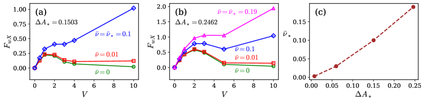
Figure 14: Non-monotonicity of the total tangential force. Figs. (a) and (b) show the total normalized force $F_{wX}$ as a function of $V$ for different values of $\bar{\nu}$ . (a) $\Delta A_{*}=0.1503$, (b) $\Delta A_{*}=0.2462$. Fig. (c) shows the estimated value $\bar{\nu}_{*}$ (above which the total force is monotonic), as a function of $\Delta A_{*}$.

The total force is the sum of the membrane contribution with the viscous force of the liquid which is proportional to the shear rate. Combining Eqs. (7,20), we have

$$f_{wx}=\frac{\mathcal{U}_{0}^{\frac{5}{4}}}{24\kappa^{\frac{1}{4}}h_{0}^{\frac{1}{2}}}\left[\bar{\nu}V+12\langle H\partial_{X}HF_{Z}\rangle\right].$$ (73)

The dimensionless parameter $\bar{\nu}=12\kappa^{1/2}\mu\nu/(\mathcal{U}_{0}^{1/2}h_{0}^{2})$ governs the balance between the membrane contribution and the bulk liquid viscous force. Small $\bar{\nu}$ means that the membrane contributes significantly to the global friction while large $\bar{\nu}$ means that friction is dominated by viscous dissipation in the liquid. However, as discussed in Ref.To et al. (2018), the parameter $\bar{\nu}$ also accounts for the distinction between the limit of permeable walls for $\bar{\nu}\gg 1$ where our dynamical model Eq. (2) apply, and the limit of impermeable walls $\bar{\nu}\ll 1$ where instead, a different model accounting for a fluid flow which is mainly parallel to the membrane, must be used. This latter conserved model has been described in Ref.To et al. (2018). In the present work, we focus on the limit of permeable walls so that $\bar{\nu}\gg 1$.

As reported above, the membrane contribution to the force on the walls exhibits a non monotonic variation as a function of the shear rate. Indeed, it decreases in regime II. Using the normalized equation (20), we see that the total force can also be decreasing in regime II if $\bar{\nu}<-12\partial_{V}\langle H\partial_{X}HF_{z}\rangle$. As seen in Fig. 14(a), such a condition can for example be achieved when $\bar{\nu}<10^{-1}$ for $\Delta A_{*}=0.1503$. We define the value $\bar{\nu}_{*}$ of $\bar{\nu}$ for which the total force changes from non-monotonic to monotonic variation. Fig. 14(c) shows that $\bar{\nu}_{*}$ increases almost linearly with $\Delta A_{*}$.

Since $\bar{\nu}\gg 1$ in the case of permeable walls, a non-monotonic dependence of the total force on the shear rate cannot be achieved for small normalized excess area. We do not have detailed data at large excess area. However, an extrapolation of the value of $\bar{\nu}_{*}$ to larger excess area suggests that $\bar{\nu}_{*}>1$ roughly when $\Delta A_{*}>1$. As a consequence, a non-monotonic behavior could be obtained at larger excess area. Such a non-monotonic behavior was already suggested in the 1D model of Ref.Le Goff et al. (2017) in the impermeable limit, and could lead to instabilities such as stick-slip.

Let us now discuss quickly the orders of magnitude of relevant physical parameters. The typical bending rigidity of lipid membrane is $\kappa\sim 10^{-19}~{}\mathrm{J}$Henriksen et al. (2006); Pakkanen et al. (2011). Moreover, several experiments Bruinsma et al. (2000); Weikl et al. (2009); Sengupta and Limozin (2010) suggest that the typical distance $h_{0}$ with the walls is a few nanometers in biological systems. We also consider that the fluid surrounding the membrane is water with a viscosity $\mu\sim 10^{-3}~{}\mathrm{Pa.s}$. For walls such as collagen Miron-Mendoza et al. (2010) or the cytoskeleton, the order of magnitude of the permeability can be evaluated as $\nu\sim~{}10^{-5}~{}\mathrm{m}^{2}.\mathrm{s}.\mathrm{kg}^{-1}$ using Darcy’s law. The order of magnitude of the potential varies also strongly with the nature of the interaction. In order to determine $\mathcal{U}_{0}$, we use the difference $\Delta\mathcal{U}=\mathcal{U}(h=0.9h_{0})-\mathcal{U}(h=0)$ of potential between the potential in the center at $h=0$, and close to the walls at $h=0.9h_{0}$. In the case of hydration forces we obtain $\mathcal{U}_{0}\sim 10^{-2}-10^{-1}~{}\mathrm{J}.\mathrm{m}^{-2}$ Swain and Andelman (2001); Schneck et al. (2012). These numbers suggest $\bar{\nu}\sim 10$, and are therefore consistent with the case of permeable walls. In addition, this leads to $\ell_{\parallel}\sim h_{0}$ and $\epsilon\sim 1$. This means that the units of the wrinkle wavelength $\lambda$ in Fig. 4(b) is about $10$nm. Furthermore, an inspection of Fig. 4(b) indicates that the small slope approximation, where $\lambda\gg h_{0}$ should be valid only when $\Delta A_{*}\ll 1$. Hence, the excess area in physical coordinates $\Delta{\cal A}/({\cal L}_{x}{\cal L}_{y})=\epsilon\Delta A_{*}\sim\Delta A_{*}$ should be small. Although the fact that $\epsilon\sim 1$ questions the strict validity of the small slope limit for larger excess areas, our model should grasp some features of the dynamics of lubricated contacts with membranes for small excess areas.

VIII.3 Conclusion

As a summary, we have presented a lubrication model which describes the dynamics of an inextensible membrane in an incompressible fluid between two walls. In quiescent conditions, the membrane forms a frozen labyrinthine pattern of wrinkles which stores the membrane excess area. When shear flow is induced by the parallel motion of the walls, the wrinkles reorganize leading to a nonlinear rheological response of the system.

Our results show how the excess area of the membrane participates in a non-trivial way to the rheology of contacts containing lipid membranes. One important difference as compared to our previous investigations of confined membranes is that we have considered confinement by a single-well potential here as compared to the double-well confinement potential used in our previous studies Le Goff et al. (2017); To et al. (2018). As a consequence of this difference, we observe no coarsening here, while coarsening in the presence of a double-well potential was shown to be at the origin of thixotropic behavior in Ref. Le Goff et al. (2017). These results show that the rheological response of lubricated contacts containing membranes could be controlled by the details of the confinement potential.

Finally, although our simple model catches a complex behavior from a set of simple physical ingredients, much yet remains to be done to describe the role of membranes in specific biolubrication systems. In particular, possible future extensions of our work include the cases of impermeable walls and of stacks of several membranes. In addition, one could study the role of thermal fluctuations, e.g. following a Langevin approach as in Ref. Le Goff et al. (2014).

Author contributions

TLG and TBTT have contributed equally to the manuscript. Conceptualization: OPL. Formal analysis and Writing: TLG, TBTT and OPL. Software: TBTT and TLG.

Conflicts of interest

There are no conflicts to declare.

Appendix A Derivation of the force on the walls

A.1 Hydrodynamic flow

In the lubrication approximation, the components of the fluid velocity $\upsilon_{x},\upsilon_{y}$ take the form of a Poiseuille flow To et al. (2018)

$$\upsilon_{x\pm}=\frac{z^{2}}{2\mu}\partial_{x}p_{\pm}+a_{x\pm}z+b_{x\pm},\quad\upsilon_{y\pm}=\frac{z^{2}}{2\mu}\partial_{y}p_{\pm}+a_{y\pm}z+b_{y\pm},$$ (74)

where $\pm$ denotes the liquid above or below the membrane. The ten quantities $p_{\pm},a_{x\pm},a_{y\pm},b_{x\pm},b_{y\pm}$ are functions of $x$ and $y$, and are constants with respect to $z$. The fluid velocity at the two walls and at the membrane satisfy a no-slip condition

$$\upsilon_{x\pm}\rvert_{z=\pm h_{0}}=\pm\upsilon_{0},\quad\upsilon_{y\pm}\rvert_{z=\pm h_{0}}=0,$$ (75)

$$\upsilon_{x+}\rvert_{z=h}=\upsilon_{x-}\rvert_{z=h},\quad\upsilon_{y+}\rvert_{z=h}=\upsilon_{y-}\rvert_{z=h}.$$ (76)

Moreover, the tangential stresses are assumed to be continuous across the membrane

$$\partial_{z}\upsilon_{x+}\rvert_{z=h}=\partial_{z}\upsilon_{x-}\rvert_{z=h},\quad\partial_{z}\upsilon_{y+}\rvert_{z=h}=\partial_{z}\upsilon_{y-}\rvert_{z=h}.$$ (77)

In addition, the normal force $f_{z}$ which is oriented along $z$ to leading order balances the difference of pressure above and below the membrane

$$p_{+}-p_{-}=f_{z}.$$ (78)

A.2 Tangential forces

The tangential forces on the walls are due to the viscous shear stress exerted by the fluid on the wall. The two components of the friction force per unit area are given by the difference of shear stresses on the upper and lower walls

$$f_{wx}=\frac{\mu}{{\cal L}_{x}{\cal L}_{y}}\int_{0}^{{\cal L}_{x}}dx\int_{0}^{{\cal L}_{y}}dy\left(\partial_{z}\upsilon_{x+}\rvert_{z=+h_{0}}+\partial_{z}\upsilon_{x-}\rvert_{z=-h_{0}}\right),$$

$$f_{wy}=\frac{\mu}{{\cal L}_{x}{\cal L}_{y}}\int_{0}^{{\cal L}_{x}}dx\int_{0}^{{\cal L}_{y}}dy\left(\partial_{z}\upsilon_{y+}\rvert_{z=+h_{0}}+\partial_{z}\upsilon_{y-}\rvert_{z=-h_{0}}\right).$$ (79)

Substituting the expression of the hydrodynamic velocity Eq. (74) in the boundary conditions Eqs. (75-78) and combining these expressions, we obtain

$$\left(\partial_{z}\upsilon_{x+}\rvert_{z=+h_{0}}+\partial_{z}\upsilon_{x-}\rvert_{z=-h_{0}}\right)=2\frac{v_{0}}{h_{0}}+\frac{h^{2}-h_{0}^{2}}{2\mu h_{0}}\partial_{x}f_{z},$$

$$\left(\partial_{z}\upsilon_{y+}\rvert_{z=+h_{0}}+\partial_{z}\upsilon_{y-}\rvert_{z=-h_{0}}\right)=\frac{h^{2}-h_{0}^{2}}{2\mu h_{0}}\partial_{x}f_{z}.$$ (80)

Inserting these expressions into Eq. (A.2) leads to Eqs. (7,II.2).

A.3 Dynamical equation

In order to determine the ten functions $p_{\pm},a_{x\pm},a_{y\pm},b_{x\pm},b_{y\pm}$, the seven boundary conditions Eqs. (75-78) are not sufficient.

Additional boundary conditions at the walls and at the membrane involve vertical flow. The vertical motion of the interface is associated to vertical hydrodynamic flows

$$u_{z+}\rvert_{z=h}=\partial_{t}h,\quad u_{z-}\rvert_{z=h}=\partial_{t}h.$$ (81)

Vertical hydrodynamic flows at the walls are caused by flow through the porous walls  To et al. (2018); Le Goff et al. (2014)

$$u_{z+}\rvert_{z=+h_{0}}=\nu(p_{+}-p_{eq}),\quad u_{z-}\rvert_{z=-h_{0}}=-\nu(p_{-}-p_{eq}),$$ (82)

where $p_{eq}$ is a reference pressure.

In the lubrication expansion, vertical flow in the $z$ direction is smaller than the flow in the $x,y$ plane, and appears to higher order. However, vertical flows are crucial and balance the large-scale variations of the horizontal flow in mass conservation.

Since we have four additional relations Eqs. (81,82), we have in total eleven relations and ten unknowns. We therefore find the expression of all the unknown, plus one evolution relating $\partial_{t}h$ and the other physical quantities. This leads to complex expressions in general, and detailed derivations are reported in Ref. To et al. (2018); Le Goff et al. (2014). In the limit of large $\bar{\nu}$, one obtains Eq. (2).

A.4 Limit $\bar{\nu}\gg 1$

Here, we report a heuristic discussion of the meaning of the parameter $\bar{\nu}$, and of the limit $\bar{\nu}\gg 1$. Let us discard the shear flow created by the motion of the walls for simplicity. First, we notice that since the hydrodynamic velocity in the $(x,y)$ plane is a Poiseuille flow, which is quadratic in $z$ from Eq. (74), the total flow $\mathbf{j}=(j_{x},j_{y})$ integrated over $z$ is cubic in $h_{0}$, i.e. $j\sim(h_{0}^{3}/\mu)\nabla_{xy}p$. The motion of the membrane can either result from a non-constant flow above or below, leading to $\partial_{t}h\sim-\nabla_{xy}\cdot\mathbf{j}$, or from the loss of mass through the permeable walls, leading to $\partial_{t}h\sim\nu(p-p_{eq})$. These correspond to two different dissipation mechanisms controlled by the kinetic coefficients $\mu$ and $\nu$. Assume now that we consider a membrane pattern with a lengthscale $\ell$ in the $x,y$ plane. Then, $\nabla_{xy}\sim 1/\ell$, and $\nabla_{xy}\cdot\mathbf{j}\sim(h_{0}^{3}/\mu)p/\ell^{2}$. Hence, the motion of the membrane is limited by hydrodynamic flow parallel to the walls when $(h_{0}^{3}/\mu)p/\ell^{2}\gg\nu(p-p_{eq})$, and limited by the flow through the walls in the opposite limit. Eliminating $p$, we obtain viscosity-limited motion for $\ell\ll\ell_{kin}$ and permeability-limited regime for $\ell\gg\ell_{kin}$, where

$$\ell_{kin}=\left(\frac{h_{0}^{3}}{\mu\nu}\right)^{1/2}.$$ (83)

Choosing the natural lengthscale of the pattern $\ell\sim\ell_{\parallel}$ defined in Eq. (11), we obtain the viscosity-limited motion for $\bar{\nu}\ll 1$ and permeability-limited regime for $\bar{\nu}\gg 1$, where $\bar{\nu}$ is defined in Eq. (1).

Two remarks are in order. First, our analysis in this paper focuses on the permeability-limited regime for $\bar{\nu}\gg 1$ which corresponds to patterns that exhibit a lengthscale larger than $\ell_{kin}$. Second, the parameter $\nu$ does not compare vertical and horizontal hydrodynamic velocities. Indeed, from Eq. (74), horizontal velocities scale as $h_{0}^{2}p/(\mu\ell)$, vertical velocities scale as $\nu(p-p{eq})$. Their ratio reads $\ell\mu\nu/h_{0}^{2}\sim\bar{\nu}(h_{0}/\ell)$. Since $\epsilon=h_{0}/\ell$ is small from the very definition of the lubrication approximation, the vertical hydrodynamic velocities are always smaller than the horizontal ones. In addition, the strict validity of the lubrication approximation requires that $\bar{\nu}\epsilon$ should be small even when $\bar{\nu}$ is large, i.e. that $\epsilon$ is smaller than $\bar{\nu}^{-1}$.

Appendix B Sine-profile ansatz without shear

B.1 General procedure

Let $\zeta$ be the variable in the direction perpendicular to the wrinkles. We assume that the membrane profile is sinusoidal $H(\zeta)=a\cos(q\zeta)$ where $a$ is the amplitude and $q$ is the wave number $q=2\pi/\lambda$, $\lambda$ is the wavelength of the wrinkle. Using this ansatz the relation between the amplitude $a$ and the root-mean-square amplitude $\langle H^{2}\rangle$ is $a=\sqrt{2}\langle H^{2}\rangle^{\frac{1}{2}}$.

Consider the free energy $\xi$ per unit length of one straight wrinkle:

$$\xi=\int_{0}^{\lambda}d\zeta\left\{\frac{1}{2}(\partial_{\zeta\zeta}H)^{2}+\frac{\Sigma_{0}}{2}(\partial_{\zeta}H)^{2}+U(H)\right\},$$ (84)

where the tension $\Sigma_{0}$ accounts for the constraint of fixed total excess area. Substituting the sine ansatz, we obtain

$$\xi=\frac{2\pi}{q}\left\{\frac{1}{4}(a^{2}q^{4}+a^{2}q^{2}\Sigma_{0})+J_{U}\right\}.$$ (85)

The free energy density (i.e. the free energy per unit area) is then given by

$$\bar{\xi}=\frac{\xi}{\lambda}=\frac{1}{4}(a^{2}q^{4}+a^{2}q^{2}\Sigma_{0})+J_{U},$$ (86)

where

$$J_{U}=\frac{1}{2\pi}\int_{0}^{2\pi}d\eta U(H).$$ (87)

Here we have defined the integration variable $\eta=q\zeta$.

To find the wavelength $\tilde{\lambda}=2\pi/\tilde{q}$ and the amplitude $\tilde{a}$ that minimize the energy density $\bar{\xi}$, we first minimize $\bar{\xi}$ with respect to $q$. Solving $\partial_{q}\bar{\xi}=0$ we obtain the relation $\Sigma_{0}=-2\tilde{q}^{2}$. Thus, we have

$$\left.\bar{\xi}\right\rvert_{q=\tilde{q}}=-\frac{1}{4}a^{2}\tilde{q}^{4}+J_{U}.$$ (88)

Next we minimize $\left.\bar{\xi}\right\rvert_{q=\tilde{q}}$ with respect to $a$. Solving $\partial_{a}\left(\left.\bar{\xi}\right\rvert_{q=\tilde{q}}\right)=0$ we find the dependence of $\tilde{q}$ on $\tilde{a}$

$$\tilde{q}=\left[\frac{2}{\tilde{a}}\left.(\partial_{a}J_{U})\right\rvert_{a=\tilde{a}}\right]^{\frac{1}{4}}.$$ (89)

To establish this relation, we have used the fact that since $U(H)$ depends only on $H$ and not on its spatial derivatives, $J_{U}$ depends only on $a$, and not on $q$. Note in addition that we could have also obtained this relation by direct substitution of the relation $\Sigma_{0}=-2\tilde{q}^{2}$ into Eq. (17).

A relation between $\tilde{a}$ and the membrane excess area $\Delta A_{*}$ is then obtained from evaluation of the excess area with the sine-profile ansatz,

$$\Delta A_{*}=\left(\frac{\tilde{q}\tilde{a}}{2}\right)^{2}=\left[\frac{\tilde{a}^{3}}{8}\left.(\partial_{a}J_{U})\right\rvert_{a=\tilde{a}}\right]^{\frac{1}{2}}.$$ (90)

As a summary, the amplitude $a$ can be calculated from the excess area $\Delta A_{*}$ from the inversion of Eq. (90). Then, the wavelength of the wrinkles is obtained as a function of $a$ using Eq. (89).

B.2 Case of the potential $U(H)=(1-H^{p})^{-m}$

In order to find $\tilde{q}$ and $\tilde{a}$ more explicitly we need to calculate $J_{U}$ and $\partial_{a}J_{U}$ for a given $U(H)$. Consider the energy potential of the general form

$$U(H)=(1-H^{p})^{-m},$$ (91)

where $p$ is a positive even integer and $m$ is a positive integer. We then have

$$J_{U} =1+\sum_{k=1}^{\infty}{m+k-1\choose k}I_{pk}a^{pk},$$

$$\partial_{a}J_{U} =\frac{p}{a}\sum_{k=1}^{\infty}{m+k-1\choose k}kI_{pk}a^{pk}.$$ (92)

We have defined

$$I_{pk}=\frac{1}{2\pi}\int_{0}^{2\pi}d\eta\cos^{pk}\eta=\frac{1}{\pi}B\left(\frac{1}{2},\frac{1}{2}+\frac{pk}{2}\right),$$ (93)

where $B(x,y)$ is the Beta function. Finally, we obtain

$$\tilde{q} =\left[\frac{2p}{\tilde{a}^{2}}\sum_{k=1}^{\infty}{m+k-1\choose k}kI_{pk}\tilde{a}^{pk}\right]^{\frac{1}{4}},$$

$$\Delta A_{*} =\left[\frac{p}{8}\sum_{k=1}^{\infty}{m+k-1\choose k}kI_{pk}\tilde{a}^{pk+2}\right]^{\frac{1}{2}}.$$ (94)

The results of Eqs. (B.2) is shown in Fig. 15 for some values of $m$ and $p$.

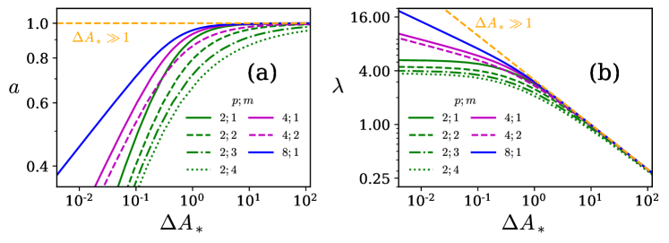
Figure 15: Predictions of the sine-ansatz Eq. (B.2). (a) Wrinkle amplitude $a$ and (b) wrinkle wavelength $\lambda$ of the membrane profile as a function of the normalized excess area for various values of $m$ and $p$ using the potential $U(H)=(1-H^{p})^{-m}$. The yellow dashed lines show the analytical results for large excess area Eq. (26): $a=1$ and $\lambda=\pi\Delta A_{*}^{-1/2}$.

B.3 Limit of small amplitudes for the potential $U(H)=(1-H^{p})^{-m}$

For small amplitudes $a$, we only keep the first term in the series expansion of Eq. (B.2)

$$\tilde{q} =\left(2mpI_{p}\tilde{a}^{p-2}\right)^{\frac{1}{4}},$$

$$\Delta A_{*} =\left(\frac{pm}{8}I_{p}\tilde{a}^{p+2}\right)^{\frac{1}{2}},$$ (95)

where we have defined the constant

$$I_{p}=I_{pk}\rvert_{k=1}=\frac{1}{\pi}B\left(\frac{1}{2},\frac{1}{2}+\frac{p}{2}\right).$$ (96)

We finally obtain

$$\tilde{a} =\Delta A_{*}^{\frac{2}{p+2}}C_{m,p},$$

$$\tilde{q} =2\Delta A_{*}^{\frac{1}{2}-\frac{2}{p+2}}(C_{m,p})^{-1},$$

$$\tilde{\lambda} =\frac{2\pi}{\tilde{q}}=\Delta A_{*}^{-\frac{1}{2}+\frac{2}{p+2}}\pi C_{m,p},$$ (97)

where we have defined

$$C_{m,p}=\left(\frac{8}{mpI_{p}}\right)^{\frac{1}{p+2}}.$$ (98)

Appendix C Random initial conditions

Our simulation scheme with area conservation requires a random smooth initial condition for the excess area to be well defined. Such an initial condition with excess area $\Delta A_{*}$ can be obtained by solving the time-dependent Ginzburg-Landau (TDGL) equation

$$\partial_{T}H=w^{2}\Delta H-U_{\mathrm{adh}}^{\prime}(H),$$ (99)

using an explicit scheme with finite-differences and random initial conditions. We use a double-well adhesion potential To et al. (2018)

$$U_{\mathrm{adh}}=\frac{1}{4}(H_{m}^{2}-H^{2})^{2}.$$ (100)

Membrane profiles with different excess areas $\Delta A_{*}$ can be selected (as initial conditions for the main simulations) by varying the potential well $H_{m}$ ($H_{m}<1$), the domain width $w$ (typically $w<1$), and the simulation time of the TDGL equation (typically between 10 and 30). In our previous work, we have obtained evidences that such a procedure does not affect the details of the subsequent dynamics To et al. (2018).

Appendix D Numerical evaluation of the drift velocity

In this appendix, we report on the numerical evaluation of the drift velocity of drifting steady-states $\mathbf{V}_{d}$ with its two components $V_{dX}$ and $V_{dY}$. In order to validate the method, we first perform a direct measurement on the images of the drift velocity of some defect. We refer to this method as Method 1 and denote the velocity as $V_{d1X}$ and $V_{d1Y}$ of the membrane profile.

The drift velocity can also be evaluated numerically as follows. A drifting steady-state obeys

$$-V_{dX}\partial_{X}H-V_{dY}\partial_{Y}H=F_{Z}-VH\partial_{X}H.$$ (101)

We multiply Eq. (101) with an arbitrary function $\phi(H)$ and integrate over $X$ to obtain

$$V_{dY}=-\frac{\int dX[\phi(H)F_{Z}]}{\int dX[\phi(H)\partial_{Y}H]}.$$ (102)

Likewise, to calculate $V_{dX}$ we multiply Eq. (101) with an arbitrary function $\chi(H)$ and integrate over $Y$ to get

$$V_{dX}=-\frac{\int dY[\chi(H)F_{Z}]+V\int dY[\chi(H)H\partial_{X}H]}{\int dY[\chi(H)\partial_{X}H]}.$$ (103)

Note that Eq. (102) provides an evaluation of $V_{dY}$ for each value of $X$, and Eq. (103) provides an evaluation of $V_{dX}$ for each value of $Y$. The main difficulty of this method is that the denominator of Eqs. (102,103) is very small for some specific values of $Y$ or $X$, leading to numerical inaccuracies or divergences. A simple solution to this difficulty is to evaluate these expressions for all $Y$ and $X$ on our numerical spatial grid, and take the median value. We find that the resulting estimate is reliable, as shown by the comparison with direct measurements in Table 1.

$\Delta A_{*}$	$V$	$T$	$V_{d2X}$	$V_{d1X}$	$V_{d2Y}$	$V_{d1Y}$
$0.007495$	0.01	$1.99\times 10^{6}$	$6.8545\times 10^{-6}$	$7.07\times 10^{-6}$	$1.5721\times 10^{-6}$	$2.02\times 10^{-6}$
$0.007495$	0.1	$1.45\times 10^{6}$	$5.7022\times 10^{-5}$	$5.634\times 10^{-5}$	$1.7475\times 10^{-5}$	$1.878\times 10^{-5}$
$0.007495$	0.5	$5\times 10^{5}$	$-1.3988\times 10^{-3}$	$-1.4\times 10^{-3}$	$-5.0391\times 10^{-5}$	$-5.13\times 10^{-5}$
$0.007495$	1	$2\times 10^{5}$	$7.3187\times 10^{-3}$	$7.36\times 10^{-3}$	$-1.8964\times 10^{-4}$	$-2.32\times 10^{-4}$
$0.01186$	0.1	$5\times 10^{5}$	$1.0634\times 10^{-5}$	$1.05\times 10^{-5}$	$-6.1509\times 10^{-6}$	$-6.31\times 10^{-6}$
$0.01186$	0.2	$1.28\times 10^{6}$	$5.5289\times 10^{-5}$	$6.25\times 10^{-5}$	$1.8618\times 10^{-5}$	$0.947\times 10^{-5}$
$0.1503$	0.5	$5\times 10^{5}$	$3.9351\times 10^{-5}$	$3.33\times 10^{-5}$	$4.5404\times 10^{-7}$	$0$
$0.1503$	1	$4.8\times 10^{5}$	$4.853\times 10^{-4}$	$4.7083\times 10^{-4}$	$4.2342\times 10^{-5}$	$4.167\times 10^{-5}$
$0.1503$	2	$5\times 10^{5}$	$6.6394\times 10^{-4}$	$6.18\times 10^{-4}$	$-8.6122\times 10^{-5}$	$-8.94\times 10^{-5}$
$0.1503$	10	$5\times 10^{5}$	$8.0422\times 10^{-4}$	$8.42\times 10^{-4}$	$-4.8108\times 10^{-7}$	$0$
$0.2462$	5	$4\times 10^{5}$	$-5.0496\times 10^{-4}$	$-6.24\times 10^{-4}$	$-2.2137\times 10^{-5}$	$-1.44\times 10^{-5}$
$0.2462$	20	$1.5\times 10^{5}$	$2.2826\times 10^{-3}$	$2.2279\times 10^{-3}$	$6.196\times 10^{-7}$	$0$

Table 1: Drift velocity along $X$ and $Y$. $V_{d1X}$ and $V_{d1Y}$ are values from manual measurement from images. $V_{d2X}$ and $V_{d2Y}$ are medians of the calculated values using $\phi(H)=\chi(H)=1$.

References

- Trunfio-Sfarghiu et al. (2008) A.-M. Trunfio-Sfarghiu, Y. Berthier, M.-H. Meurisse, and J.-P. Rieu, Langmuir 24, 8765 (2008).
- Schmidt et al. (2007) T. A. Schmidt, N. S. Gastelum, Q. T. Nguyen, B. L. Schumacher, and R. L. Sah, Arthritis and Rheumatology 56, 882 (2007).
- Botan et al. (2015) A. Botan, L. Joly, N. Fillot, and C. Loison, Langmuir 31, 12197 (2015).
- Swann et al. (1984) D. A. Swann, K. J. Bloch, D. Swindell, and E. Shore, Arthritis and Rheumatology 27, 552 (1984).
- Tadmor et al. (2002) R. Tadmor, N. Chen, and J. N. Israelachvili, J. Biomedical Materials Research 61, 514 (2002).
- Erdemir (2005) A. Erdemir, Tribology International 38, 249 (2005), boundary Lubrication.
- Raviv et al. (2003) U. Raviv, S. Giasson, N. Kampf, J.-F. Gohy, R. Jérôme, and J. Klein, Nature 425, 163 (2003).
- Briscoe et al. (2006) W. H. Briscoe, S. Titmuss, F. Tiberg, R. K. Thomas, D. J. McGillivray, and J. Klein, Nature 444, 191 (2006).
- Gov et al. (2004) N. Gov, A. G. Zilman, and S. Safran, Phys. Rev. E 70, 011104 (2004).
- Marlow and Olmsted (2002) S. W. Marlow and P. D. Olmsted, Phys. Rev. E 66, 061706 (2002).
- Huang and Im (2006) R. Huang and S. H. Im, Phys. Rev. E 74, 026214 (2006).
- To et al. (2018) T. B. T. To, T. Le Goff, and O. Pierre-Louis, Soft Matter 14, 8552 (2018).
- Cerda and Mahadevan (2003) E. Cerda and L. Mahadevan, Phys. Rev. Lett. 90, 074302 (2003).
- Leocmach et al. (2015) M. Leocmach, M. Nespoulous, S. Manneville, and T. Gibaud, Science Advances 1, e1500608 (2015).
- Le Berre et al. (2002) M. Le Berre, E. Ressayre, A. Tallet, Y. Pomeau, and L. Di Menza, Phys. Rev. E 66, 026203 (2002).
- Le Goff et al. (2017) T. Le Goff, T. B. T. To, and O. Pierre-Louis, The European Physical Journal E 40, 44 (2017).
- Swain and Andelman (2001) P. S. Swain and D. Andelman, Phys. Rev. E 63, 051911 (2001).
- Sengupta and Limozin (2010) K. Sengupta and L. Limozin, Phys. Rev. Lett. 104, 088101 (2010).
- Israelachvili (2015) J. Israelachvili, Intermolecular and Surface Forces, Intermolecular and Surface Forces (Elsevier Science, 2015).
- Canham (1970) P. Canham, Journal of Theoretical Biology 26, 61 (1970).
- Helfrich (1973) W. Helfrich, Zeitschrift für Naturforschung C 28, 693 (01 Dec. 1973).
- Lipowsky (1995) R. Lipowsky, Current Opinion in Structural Biology 5, 531 (1995).
- Seifert (1995) U. Seifert, Zeitschrift für Physik B Condensed Matter 97, 299 (1995).
- Young et al. (2014) Y.-N. Young, S. Veerapaneni, and M. J. Miksis, Journal of Fluid Mechanics 751, 406–431 (2014).
- Sheetz (2001) M. P. Sheetz, Nature Reviews Molecular Cell Biology 2, 392 (2001).
- Speck and Vink (2012) T. Speck and R. L. C. Vink, Phys. Rev. E 86, 031923 (2012).
- Maciver (1992) S. Maciver, Trends in Cell Biology 2, 282 (1992).
- Berrier and Yamada (2007) A. L. Berrier and K. M. Yamada, Journal of Cellular Physiology 213, 565 (2007), https://onlinelibrary.wiley.com/doi/pdf/10.1002/jcp.21237 .
- Braga (2002) V. M. Braga, Current Opinion in Cell Biology 14, 546 (2002).
- Asfaw et al. (2006) M. Asfaw, B. Różycki, R. Lipowsky, and T. R. Weikl, Europhysics Letters (EPL) 76, 703 (2006).
- Note (1) The wavelength is evaluated from the simulation with the smallest value of the shear velocity that gives periodic state.
- Henriksen et al. (2006) J. Henriksen, A. Rowat, E. Brief, Y. Hsueh, J. Thewalt, M. Zuckermann, and J. Ipsen, Biophysical Journal 90, 1639 (2006).
- Pakkanen et al. (2011) K. I. Pakkanen, L. Duelund, K. Qvortrup, J. S. Pedersen, and J. H. Ipsen, Biochimica et Biophysica Acta (BBA) - Biomembranes 1808, 1947 (2011).
- Bruinsma et al. (2000) R. Bruinsma, A. Behrisch, and E. Sackmann, Phys. Rev. E 61, 4253 (2000).
- Weikl et al. (2009) T. R. Weikl, M. Asfaw, H. Krobath, B. Różycki, and R. Lipowsky, Soft Matter 5, 3213 (2009).
- Miron-Mendoza et al. (2010) M. Miron-Mendoza, J. Seemann, and F. Grinnell, Biomaterials 31, 6425 (2010).
- Schneck et al. (2012) E. Schneck, F. Sedlmeier, and R. R. Netz, Proceedings of the National Academy of Sciences 109, 14405 (2012), https://www.pnas.org/content/109/36/14405.full.pdf .
- Le Goff et al. (2014) T. Le Goff, P. Politi, and O. Pierre-Louis, Phys. Rev. E 90, 032114 (2014).