Energy-momentum tensor of the nucleon on the light front: Abel tomography case

Abstract

We investigate the two-dimensional energy-momentum-tensor (EMT) distributions of the nucleon on the light front, using the Abel transforms of the three-dimensional EMT ones. We explicitly show that the main features of all EMT distributions are kept intact in the course of the Abel transform. We also examine the equivalence between the global and local conditions for the nucleon stability in the three-dimensional Breit frame and in the two-dimensional transverse plane on the light front. We also discuss the two-dimensional force fields inside a nucleon on the light front.

I Introduction

A modern understanding of a hadronic form factor is based on the generalized parton distributions (GPDs) Mueller:1998fv ; Ji:1996ek ; Radyushkin:1996nd ; Goeke:2001tz ; Diehl:2003ny ; Belitsky:2005qn : For example, the electromagnetic form factors of the nucleon can be viewed as the first moments of the unpolarized vector GPD with respect to the parton momentum fractions. Its second moments give the nucleon gravitational form factors (GFFs) Kobzarev:1962wt ; Pagels:1966zza , which are also defined in terms of the nucleon matrix element of the energy-moment tensor (EMT). Since the EMT arises from the response of the nucleon to a change of the external space-time metric, the corresponding form factors were christened as the GFFs. These GFFs furnish essential information on the internal structure of the nucleon such as the mass and spin distributions. The most nontrivial part of the GFFs comes from the $D$-term (Druck-term) form factor Polyakov:2002yz , which is deeply related to the stability of the nucleon. It reveals how the nucleon acquires its mechanical stability, which is exhibited by the pressure and shear-force densities. These three-dimensional (3D) distributions are often presented in the Breit frame (BF) Polyakov:2002yz ; Goeke:2007fp ; Polyakov:2018zvc . In the meanwhile, there have been criticisms on the validity of the 3D densities for the nucleon Yennie:1957 ; Burkardt:2000za ; Burkardt:2002hr ; Belitsky:2005qn ; Miller:2007uy ; Miller:2010nz ; Jaffe:2020ebz since the experiments on the proton structure performed by Hofstadter Hofstadter:1956qs ; Hofstadter:1956qs ; Hofstadter:1957wk . As pointed out in the literatures, the 3D densities are only valid for nonrelativistic particles such as atoms and nuclei, of which the intrinsic sizes are much larger than the corresponding Compton wavelengths ($\lambdabar=\hbar/mc$). When it comes to the nucleon, however, the ratio of the Compton wavelength to the radius is numerically of order $\sim 1/4$, which may result in relativistic corrections up to 20 % for the distributions and up to 10 % for the nucleon radii. Moreover, the ratio is of order $1/N_{c}$, i.e. the relativistic corrections are parametrically small in the large $N_{c}$ limit of QCD, which we employ in the present work.

The BF distributions for the static EMT can be interpreted as quasiprobabilistic densities from the phase-space perspectiveLorce:2017wkb ; Lorce:2018zpf ; Lorce:2018egm ; Lorce:2020onh ; Lorce:2021gxs . This means that the BF distributions, which are defined through the Wigner distributions in the quantum phase space Wigner:1932eb ; Hillery:1983ms , can be comprehended as quasiprobabilistic ones due to Heisenberg’s uncertainty relations. On the other hand, if one takes the infinite momentum frame (IMF), which indicates that the nucleon is on the light-front (LF), the relativistic corrections to the distributions are suppressed kinematically and a transversely localized state for the nucleon can be defined, which enables one to construct the two-dimensional (2D) transverse distributions on the LF. They provide a strict probabilistic interpretation Burkardt:2002hr ; Miller:2007uy ; Carlson:2007xd and are not Lorentz contracted, since the initial and final states of the nucleon lie on the mass shell. Recently, it was shown in Ref. Lorce:2020onh that the BF charge distributions can be interpolated to the LF ones. In Ref. Panteleeva:2021iip , this interpolation was applied to the EMT force distributions. This was realized by the Abel transform Abel that had been used in the computerized medical tomography in connection with the Radon transform Natterer:2001 . Actually, the Abel transform was already utilized in the deeply virtual Compton scattering Polyakov:2007rv ; Moiseeva:2008qd . As pointed out in Ref. Panteleeva:2021iip , thus, it is of great importance to scrutinize how the EMT force distributions in the BF are related to those in the IMF. The GFFs of the nucleon were already investigated in the chiral quark-soliton model ($\chi$QSM) Goeke:2007fp . It was shown how the nucleon acquires the stability by examining its pressure densities. The work was extended to the GFFs of the singly heavy baryon $\Sigma_{c}$ in comparison with those of the nucleon Kim:2020nug , the force fields inside the nucleon and $\Sigma_{c}$ being emphasized. Both the global and local stability conditions Perevalova:2016dln ; Polyakov:2018zvc for them were carefully examined. In the present work, we want to study how the mechanical densities obtained in Ref. Kim:2020nug can be projected onto the 2D transverse plane by the Abel transform. Consequently, we show explicitly that the global and local stability conditions are equivalently satisfied both in the BF and on the LF.

The present work is organized as follows: In Sec. II, we define the GFFs and show how the mechanical densities are derived. Then we relate the 3D distributions to the 2D ones by the Abel transform. The 2D local stability conditions are presented. In Sect. III, we discuss the numerical results for both the 3D and 2D mechanical distributions such as the energy, spin, and pressure and shear-force densities. We explicitly show that the global and local stability conditions both in the BF and on the LF are equivalent to each other. We finally visualize how the force fields are distributed inside a nucleon in the transverse plane on the LF. The last Section summarizes the present results and draws conclusions.

II Gravitational form factors of the nucleon

The nucleon form factors of the symmetric EMT is defined as Kobzarev:1962wt ; Pagels:1966zza

$$\langle p^{\prime},\lambda^{\prime}|\hat{T}^{\mu\nu}(0)|p,\lambda\rangle=\overline{u}_{\lambda^{\prime}}(p^{\prime})\left[A(t)\frac{P^{\mu}P^{\nu}}{m}+J(t)\frac{iP^{\{\mu}\sigma^{\nu\}\alpha}\Delta_{\alpha}}{m}+\frac{D(t)}{4m}(\Delta^{\mu}\Delta^{\nu}-g^{\mu\nu}\Delta^{2})\right]u_{\lambda}(p)\,,$$ (1)

where $\hat{T}^{\mu\nu}(0)$ denotes the symmetric EMT operator. The parenthesis $a^{\{\mu}b^{\nu\}}=(a^{\mu}b^{\nu}+a^{\nu}b^{\mu})/2$ stand for the symmetrization operator. ${u}_{\lambda}(p)$ is the Dirac spinor. Here, $\lambda(\lambda^{\prime})$ represents the initial (final) spin projections. The normalization of Dirac spinors is taken to be $\overline{u}_{\lambda^{\prime}}(p)u_{\lambda}(p)=2m\delta_{\lambda^{\prime}\lambda}$. We use the covariant normalization $\langle p^{\prime},\lambda^{\prime}|p,\lambda\rangle=2p^{0}(2\pi)^{3}\delta_{\lambda^{\prime}\lambda}\delta^{(3)}(\bm{p}^{\prime}-\bm{p})$ of one-particle states, and introduce kinematical variables $P^{\mu}=(p^{\mu}+p^{\prime\mu})/2$, $\Delta^{\mu}=p^{\prime\mu}-p^{\mu}$ and $\Delta^{2}=t$. The nucleon matrix element of the EMT current is parametrized in terms of the three real form factors, i.e., $A(t)$, $J(t)$, and $D(t)$, which yield information on the mass, spin, and the stability of the nucleon, respectively. The mass form factor $M(t)$ is obtained in terms of these three form factors

$$M(t)=A(t)-\frac{t}{4m^{2}}\bigg{(}A(t)-2J(t)+D(t)\bigg{)}.$$ (2)

The mass $\varepsilon(r)$, angular momentum $\rho_{J}(r)$, pressure $p(r)$ and shear force $s(r)$ distributions in the BF are derived by the 3D inverse Fourier transform of the GFFs, i.e., $F=A,M,J,D$, in terms of the multipole expansion Lorce:2018egm ; Polyakov:2018zvc ; Polyakov:2018rew ; Kim:2020lrs :

$$\varepsilon(r)=m\tilde{M}(r),\ \ \rho_{J}(r)=-\frac{1}{3}r\frac{d}{dr}\tilde{J}(r),\ \ s(r)=-\frac{1}{4m}r\frac{d}{dr}\frac{1}{r}\frac{d}{dr}\tilde{D}(r),\ \ p(r)=\frac{1}{6m}\frac{1}{r^{2}}\frac{d}{dr}r^{2}\frac{d}{dr}\tilde{D}(r),$$ (3)

with the generic 3D Fourier transform

$$\tilde{F}(r)=\int\frac{d^{3}\bm{\Delta}}{(2\pi)^{3}}e^{-i\bm{\Delta}\cdot\bm{r}}F(-\bm{\Delta}^{2})\ \ .$$ (4)

As pointed out in Ref. Yennie:1957 , The physical meaning of the 3D distributions is hampered by ambiguous relativistic corrections to them. This ambiguity can be removed by considering the 2D transverse distributions in the IMF Burkardt:2000za ; Burkardt:2002hr ; Belitsky:2005qn ; Miller:2007uy ; Miller:2010nz ; Jaffe:2020ebz .

Recently, the EMT distributions in the IMF have been extensively explored in Refs. Lorce:2018egm ; Freese:2021czn ; Lorce:2017wkb ; Schweitzer:2019kkd ; Lorce:2018egm ; Panteleeva:2021iip ; Freese:2021czn . The corresponding 2D distributions for the momentum $\varepsilon^{(2D)}(x_{\perp})$, angular momentum $\rho_{J}^{(2D)}(x_{\perp})$, pressure $p^{(2D)}(x_{\perp})$ and shear force $s^{(2D)}(x_{\perp})$ are obtained by the 2D inverse Fourier transform

$$\varepsilon^{(2D)}(x_{\perp})=P^{+}\tilde{A}(x_{\perp}),\ \ \ \rho^{(2D)}_{J}(x_{\perp})=-\frac{1}{2}x_{\perp}\frac{d}{dx_{\perp}}\tilde{J}(x_{\perp}),$$ (5)

$$s^{(2D)}(x_{\perp})=-\frac{1}{4P^{+}}x_{\perp}\frac{1}{dx_{\perp}}\frac{1}{x_{\perp}}\frac{d}{dx_{\perp}}\tilde{D}(x_{\perp}),\ \ \ p^{(2D)}(x_{\perp})=\frac{1}{8P^{+}}\frac{1}{x_{\perp}}\frac{d}{dx_{\perp}}x_{\perp}\frac{d}{dx_{\perp}}\tilde{D}(x_{\perp}),$$ (6)

where we define generically the 2D Fourier transform of the corresponding GFFs as follows

$$\tilde{F}(x_{\perp})=\int\frac{d^{2}\bm{\Delta}_{\perp}}{(2\pi)^{2}}e^{-i\bm{\Delta}_{\perp}\cdot\bm{x_{\perp}}}F(-\bm{\Delta}^{2}_{\perp}).$$ (7)

The $\bm{x}_{\perp}$ and $\bm{\Delta}_{\perp}$ denote the position and momentum vectors in the 2D plane transverse to the moving direction of the nucleon, respectively. $P^{+}$ is the light-cone momentum. Note that the mass, shear force, and pressure distributions are redefined by multiplying the Lorentz factors for convenience Panteleeva:2021iip respectively as follows:

$$\mathcal{E}(x_{\perp})=\frac{m}{P^{+}}\varepsilon^{(2D)}(x_{\perp}),\ \ \mathcal{S}(x_{\perp})=\frac{P^{+}}{2m}s^{(2D)}(x_{\perp}),\ \ \mathcal{P}(x_{\perp})=\frac{P^{+}}{2m}p^{(2D)}(x_{\perp}).$$ (8)

Since the longitudinal boost does not mix the longitudinal component of the angular momentum, its distribution does not need to have an additional Lorentz factor Lorce:2017wkb . The distributions in the BF and on the LF, respectively given in Eq. (3) and Eq. (8), can be related to each other. Interestingly, the connection between those distributions turns out to be the well-known Abel transforms as follows:

$$\left(1-\frac{\partial^{2}_{(2D)}}{4m^{2}}\right)\mathcal{E}(x_{\perp}) =2\int^{\infty}_{x_{\perp}}\frac{rdr}{\sqrt{r^{2}-x^{2}_{\perp}}}\left[\varepsilon(r)+\frac{3}{2}p(r)+\frac{3}{2m}\frac{1}{r^{2}}\frac{d}{dr}r\rho_{J}(r)\right],$$ (9)

$$\rho^{(2D)}_{J}(x_{\perp}) =3\int^{\infty}_{x_{\perp}}\frac{\rho_{J}(r)}{r}\frac{x^{2}_{\perp}dr}{\sqrt{r^{2}-x^{2}_{\perp}}},$$ (10)

$$\mathcal{S}(x_{\perp}) =\int^{\infty}_{x_{\perp}}\frac{s(r)}{r}\frac{x^{2}_{\perp}dr}{\sqrt{r^{2}-x^{2}_{\perp}}},$$ (11)

$$\frac{1}{2}\mathcal{S}(x_{\perp})+\mathcal{P}(x_{\perp}) =\frac{1}{2}\int^{\infty}_{x_{\perp}}\left(\frac{2}{3}s(r)+p(r)\right)\frac{rdr}{\sqrt{r^{2}-x^{2}_{\perp}}}.$$ (12)

The Abel transform takes the same physical meaning from the 3D distributions to the 2D ones. This means that the 2D distributions $\mathcal{E}(x_{\perp})$ and $\rho_{J}^{(2D)}(x_{\perp})$ take over the meaning of the corresponding 3D ones as to how the mass and the angular momentum of the baryon are distributed in the transverse plane, respectively. Having integrated them over $\bm{x}_{\perp}$, we arrive at

$$\int d^{2}x_{\perp}\mathcal{E}(x_{\perp})=mA(0),\ \ \ \int d^{2}x_{\perp}\rho_{J}^{(2D)}(x_{\perp})=J(0),$$ (13)

with the normalized form factor $A(0)=1$ and $J(0)=1/2$, respectively. Being similar to the radii for the 3D distributions, we can define respectively the 2D radii for the mass and the angular momentum, which are relevant to the 3D radii as

$$\langle x^{2}_{\perp}\rangle_{\mathrm{mass}}=\frac{1}{m}\int d^{2}x_{\perp}x^{2}_{\perp}\mathcal{E}(x_{\perp})=\frac{2}{3}\langle r^{2}\rangle_{\mathrm{mass}}+\frac{D(0)}{m^{2}},$$ (14)

$$\langle x^{2}_{\perp}\rangle_{J}=2\int d^{2}x_{\perp}x^{2}_{\perp}\rho^{(2D)}_{J}(x_{\perp})=\frac{4}{5}\langle r^{2}\rangle_{J}.$$ (15)

The prefactors between the moments of the 2D and 3D distributions are determined by the geometric factor given in Ref. Panteleeva:2021iip

$$\Omega_{d}=\frac{\sqrt{\pi}}{2}\frac{\Gamma\left(\frac{d+1}{2}\right)}{\Gamma\left(\frac{d+2}{2}\right)},$$ (16)

with dimension $d$.

The conservation of the EMT current also provides the 2D stability condition of the nucleon. As in the 3D case, the 2D pressure and shear force distributions are responsible for the stability condition. So, we obtain the 2D equilibrium equation from the conservation of the EMT current, which is equivalent to the 3D expression as follows:

$$p^{\prime}(r)+\frac{2s(r)}{r}+\frac{2}{3}s^{\prime}(r)=0\iff\mathcal{P}^{\prime}(x_{\perp})+\frac{\mathcal{S}(x_{\perp})}{x_{\perp}}+\frac{1}{2}\mathcal{S}^{\prime}(x_{\perp})=0.$$ (17)

As shown in Eq. (17), we find that the shear force and pressure distributions are related to each other. Moreover, the 3D and 2D distributions should also comply respectively with the 3D and 2D von Laue condition and those of its lower dimension subsystem in the nucleon as

$$\int d^{3}r\,p(r) =0\iff\int d^{2}{x}_{\perp}\mathcal{P}(x_{\perp})=0,$$ (18)

$$\int^{\infty}_{0}dr\,r\left[p(r)-\frac{1}{3}s(r)\right] =0\iff\int^{\infty}_{0}d{x}_{\perp}\left[\mathcal{P}(x_{\perp})-\frac{1}{2}\mathcal{S}(x_{\perp})\right]=0.$$ (19)

This means that the 2D von Laue conditions are satisfied if and only if the 3D ones are satisfied. Furthermore, the nontrivial local stability condition for the 3D Perevalova:2016dln and 2D  Freese:2021czn pressure and shear force distributions can be considered. The integrand in the last equation of Eq. (12) is just the 3D local stability condition, which implies the 2D local stability condition on the LF Panteleeva:2021iip

$$\frac{2}{3}s(r)+p(r)>0\iff\frac{1}{2}\mathcal{S}(x_{\perp})+\mathcal{P}(x_{\perp})>0.$$ (20)

This positivity is guaranteed by the fact that the Abel image of a positive function is also positive and vice versa. This implies that the positivity of the 3D local stability condition is equivalent to the 2D ones. Thus, it allows one directly to connect the 3D mechanical radius to the 2D one

$$\langle x^{2}_{\perp}\rangle_{\mathrm{mech}}=\frac{\int d^{2}x_{\perp}x^{2}_{\perp}\left(\frac{1}{2}\mathcal{S}(x_{\perp})+\mathcal{P}(x_{\perp})\right)}{\int d^{2}x_{\perp}\left(\frac{1}{2}\mathcal{S}(x_{\perp})+\mathcal{P}(x_{\perp})\right)}=\frac{4D(0)}{\int^{0}_{-\infty}dtD(t)}=\frac{2}{3}\langle r^{2}\rangle_{\mathrm{mech}}.$$ (21)

To specify the meaning of the pressure and shear force distributions, one considers the notion of the normal and tangential force fields that are just the eigenvalues of the stress tensor contracted with the unit radial $\bm{e}_{r}$ and tangential $\bm{e}_{\phi}$ vectors, respectively. Then the 3D and the 2D force fields on the BF and LF can be obtained by

$$F_{n}(r)=4\pi r^{2}\left[\frac{2}{3}s(r)+p(r)\right],\ \ \ F_{t}(r)=4\pi r^{2}\left[-\frac{1}{3}s(r)+p(r)\right],$$ (22)

$$F_{n}^{(2D)}(x_{\perp})=2\pi x_{\perp}\left[\frac{1}{2}\mathcal{S}(x_{\perp})+\mathcal{P}(x_{\perp})\right],\ \ \ F_{t}^{(2D)}(x_{\perp})=2\pi x_{\perp}\left[-\frac{1}{2}\mathcal{S}(x_{\perp})+\mathcal{P}(x_{\perp})\right].$$ (23)

The $D$-term can be also obtained in terms of the 3D and 2D pressure and shear force distributions as

$$D(0) =-\frac{4m}{15}\int d^{3}r\,r^{2}s(r)=m\int d^{3}r\,r^{2}p(r)$$ (24)

$$=-m\int d^{2}x_{\perp}x^{2}_{\perp}\mathcal{S}(x_{\perp})=4m\int d^{2}x_{\perp}x^{2}_{\perp}\mathcal{P}(x_{\perp}).$$ (25)

This indicates that the 2D Abel images show equivalently the mechanical structure of the nucleon as the 3D distributions do.

III EMT distributions within the chiral quark-soliton model

We now present the results for the 2D distributions in the IMF. In particular, we visualize the 2D EMT distributions that are derived from the 3D ones by the Abel transform. We will use the results for the 3D distributions in the BF, which were already obtained within the framework of the $\chi$QSM Goeke:2007fp ; Kim:2020nug . Since Refs. Goeke:2007fp ; Kim:2020nug showed in detail how the EMT distributions can be calculated in the $\chi$QSM, we will only mention briefly the model before we present the results. The $\chi$QSM is known to be a pion mean-field approach to understand the structure of the lowest-lying light and singly-heavy baryons Diakonov:1987ty ; Christov:1995vm ; Diakonov:1997sj ; Diakonov:2010tf ; Yang:2016qdz ; Kim:2018cxv . The model has been very successful in describing various properties of baryons. For example, the pressure distribution of the nucleon and its $D$-term form factor obtained from the $\chi$QSM Goeke:2007fp ; Polyakov:2018zvc were in good agreement with recent data extracted from the experiments for deeply virtual Compton scattering Burkert:2018bqq . In this sense, it is of great interest to examine the 2D distributions on the LF based on the $\chi$QSM. Thus, we take the results for the 3D distributions, i.e. $\varepsilon(r)$, $\rho_{J}(r)$, $p(r)$ and $s(r)$, which were obtained in Ref. Kim:2020nug to derive the 2D EMT distributions $\mathcal{E}(x_{\perp})$, $\rho^{(2D)}_{J}(x_{\perp})$, $\mathcal{P}(x_{\perp})$ and $\mathcal{S}(x_{\perp})$ by the Abel transforms. Note that in this work we employ the dynamical quark mass as $M=350$ MeV to keep consistency with Ref. Goeke:2007fp instead of $M=420$ MeV that was often used to compute baryonic observables quantitatively.

The 2D mass distribution given in Eq. (12) can be reduced in the large $N_{c}$ limit Goeke:2007fp ; Kim:2020nug to

$$\mathcal{E}(x_{\perp})=2\int^{\infty}_{x_{\perp}}\left(\varepsilon(r)+\frac{3}{2}p(r)\right)\frac{rdr}{\sqrt{r^{2}-x^{2}_{\perp}}}.$$ (26)

A detailed discussion on the validity of neglecting the contributions from $\partial^{2}A(t)/m$ and $\partial^{2}J(t)/m$ to the mass distribution was held in Ref. Polyakov:2018zvc . We can see in Eq. (13) that the contribution from the integration of $\mathcal{E}(x_{\perp})$ over $\bm{x}_{\perp}$ is solely due to the $\varepsilon(r)$, whereas that of the pressure $p(r)$ vanishes because of the 3D von Laue condition (19). On the other hand, as presented in Eq. (15) the 2D mass radius is expressed not only by the 3D mass radius but also by the $D$-term, which is slightly different from the case of the mechanical radius given in Eq. (21). As already shown in Ref. Panteleeva:2021iip , the expressions of 2D radii can be understood and generalized in terms of the Mellin moments of the Abel images.

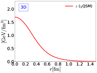
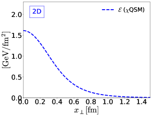
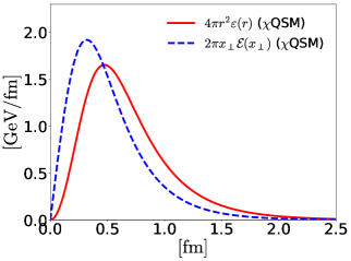
Figure 1: The solid (dashed) curve in the upper left (right) panel draws the 3D (2D) mass distributions in the BF (IMF). The solid and dashed ones in the lower panel depict respectively the 3D and 2D energy distributions weighted by $4\pi r^{2}$ and $2\pi x_{\perp}$.

We first discuss the results for the mass distributions. In the upper left and right panels of Fig. 1, we depict the results for the 3D and 2D mass distributions in the BF and IMF, respectively. The values of the mass distributions in the BF and IMF at the center are found to be $\varepsilon(0)=1.69\,\mathrm{GeV/fm}^{3}$ and $\mathcal{E}(0)=1.61\,\mathrm{GeV/fm}^{2}$. If we draw the 3D and 2D mass distributions weighted by $4\pi r^{2}$ and $2\pi x_{\perp}$ respectively, we can see that the 3D one exhibits a broader shape than the 2D ones, as illustrated in the lower panel of Fig. 1. This indicates that the 3D mass radius should be larger than the 2D one. The relative ratio between the 2D and 3D mean square mass radii is given as

$$\frac{\langle x^{2}_{\perp}\rangle_{\mathrm{mass}}}{\langle r^{2}\rangle_{\mathrm{mass}}}\approx 0.6.$$ (27)

Considering the fact that $D(0)$ should be negative, $\langle x_{\perp}^{2}\rangle_{\mathrm{mass}}$ should be smaller than $\frac{2}{3}\langle r^{2}\rangle_{\mathrm{mass}}$, as expected from Eq. (15). It is of great importance to observe that the sign of the 3D mass distribution is preserved after the Abel transform.

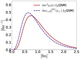
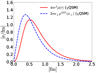
Figure 2: The solid and dashed ones in the left (right) panel depict respectively the 3D and 2D angular-momentum (charge) distributions weighted by $4\pi r^{2}$ and $2\pi x_{\perp}$ in the BF and IMF, respectively.

The solid and dashed curves in the left panel of Fig. 2 draw the 3D and 2D distributions for the angular momentum weighted by $4\pi r^{2}$ and $2\pi x_{\perp}$, respectively. As shown in Eq. (13), the 2D and 3D angular-momentum distributions are normalized as

$$\int d^{2}x_{\perp}\,\rho^{(2D)}_{J}(x_{\perp})=\int d^{3}r\,\rho_{J}(r)=J(0)=\frac{1}{2},$$ (28)

which is just the spin of the nucleon. Being similar to the case of the mass distributions, the 3D distribution is broader than the 2D one. The 2D radius for the angular-momentum distribution is related to the 3D one (15), which is smaller than the 3D radius by the geometric factor $4/5$. Thus, the 2D distribution is not much deviated from the 3D one as shown in the left panel of Fig 2. For completeness, we present the 3D and 2D charge distributions in the right panel of Fig 2. The 2D charge radius is also related to the 3D one by the geometrical factor $2/3$, i.e, $\langle x^{2}_{\perp}\rangle_{\mathrm{charge}}=\frac{2}{3}\langle r^{2}\rangle_{\mathrm{charge}}$ in the large $N_{c}$ limit.

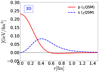
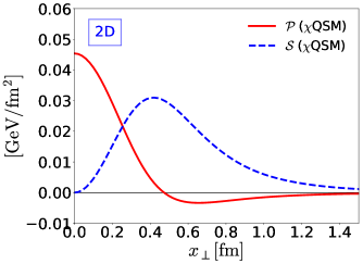
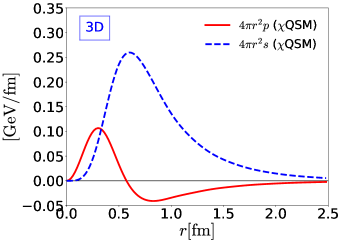
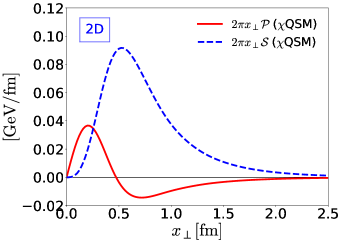
Figure 3: The upper left (right) panel presents the 3D (2D) pressure and shear-force distributions in the BF (IMF). The solid and dashed curves denote the pressure and shear-force distributions respectively. The lower left (right) panel depicts the 3D (2D) pressure and shear-force distributions weighted by $4\pi r^{2}$ $(2\pi x_{\perp})$ in the BF (IMF).

The solid and dashed curves in the upper left (right) panel of Fig. 3 show the 3D (2D) distributions for the pressure and shear force, respectively. The comparison of the 2D ones with the 3D ones provides a very important clue on the stability condition. To comply with the 3D and 2D von Laue conditions, both the 3D and 2D pressure distributions should have at least one nodal point $r_{0}$ and $(x_{\perp})_{0}$, respectively. The nodal points for the 3D and 2D pressure distributions are located at $r_{0}=0.57$ fm and $(x_{\perp})_{0}=0.47$ fm. As discussed already in Refs. Goeke:2007fp ; Kim:2020nug , the core part of $p(r)$ is governed by the contribution from the level quarks and becomes positive over the whole region of $r$, whereas the outer part is dominated by the Dirac continuum and becomes negative. This key feature of the pressure distribution explains how the nucleon acquires the stability. Interestingly, the 2D pressure distribution preserves this significant characteristic of the 3D one. The lower left (right) panel of Fig. 3 represents the 3D (2D) distributions for the pressure and shear force distributions weighted by $4\pi r^{2}$ and $2\pi x_{\perp}$, respectively, in which the key feature of the pressure distributions is amplified. It is instructive to compare the ratios of the mass, charge, angular and mechanical radii each other:

$$\langle x_{\perp}^{2}\rangle_{\mathrm{mass}}<\langle x_{\perp}^{2}\rangle_{\mathrm{mech}}<\langle x_{\perp}^{2}\rangle_{\mathrm{charge}}<\langle x_{\perp}^{2}\rangle_{J}\;\;\;(\mathrm{2D}\ \chi\mathrm{QSM})$$ (29)

$$\langle r^{2}\rangle_{\mathrm{mech}}<\langle r^{2}\rangle_{\mathrm{mass}}<\langle r^{2}\rangle_{\mathrm{charge}}<\langle r^{2}\rangle_{J}\;\;\;\;\;\;\;\;(\mathrm{3D}\ \chi\mathrm{QSM})$$ (30)

The explicit values of the radii are listed in Table 1. The size of the 3D mass distribution is larger than the 3D mechanical distribution. Interestingly, this inequality of those 2D distributions is reversed. This can be easily understood by the reason that in the case of the 2D mass distribution in the IMF is solely determined by the form factor $A(0)$ whereas the 3D mass distribution is related to the form factor $A(0)$ and $D(0)$.

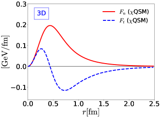
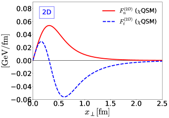
Figure 4: The solid and dashed curves in the left panel draw respectively the 3D normal and tangential force fields, i.e., $F_{n}(r),\,F_{t}(r)$) in the BF, whereas those in the right panel depict respectively their counterparts $F^{(2D)}_{n}(x_{\perp})$ and $F^{(2D)}_{t}(x_{\perp})$ in the IMF.

In the left (right) panel of Fig. 4, the solid and dashed curves depict the 3D (2D) distributions for the normal and tangential forces, respectively. Indeed, the normal force field complies with the local stability condition (20) and the tangential force satisfies the von Laue condition for the 1D subsystem (19). Due to this, both the 2D and 3D tangential forces have at least one nodal point, which means that the direction of vector fields is reversed at this point. Note that the 3D and 2D tangential forces change its direction at $r=0.44\,\mathrm{fm}$ and $x_{\perp}=0.32\,\mathrm{fm}$.

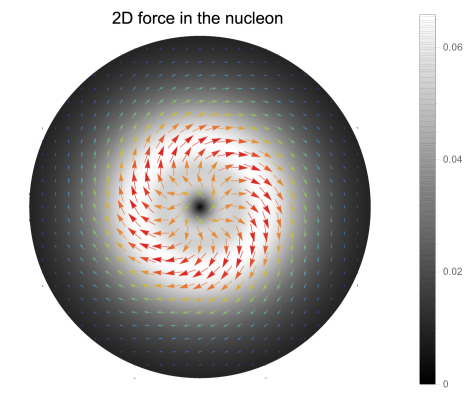
Figure 5: 2D visualization of the strong force field as a vector field inside the nucleon in the unit of $\mathrm{GeV\cdot fm^{-1}}$.

To see more clearly, the total strong force field is visualized in Fig. 5. The inner part of the strong forces is governed by the normal force, whereas the outer part is dominated by the tangential force, which ensures the nucleon to be stable. The dominance of $F_{t}$ at large distances can be obtained in the model-independent way if one uses the large $r$ behavior of the pressure and shear force distributions derived in Ref. Alharazin:2020yjv .

Table 1: Various observables of the EMT distributions for the nucleon in both the IMF and BF are listed: the energy distributions at the center $(\varepsilon(0),\,\mathcal{E}(0))$, the pressure distributions at the center $(p(0),\,\mathcal{P}(0))$, nodal points of the pressures $((x_{\perp})_{0},\,r_{0})$ and the mean square radii of the mass, angular momentum, mechanical and charge ($\langle r^{2}\rangle,\,\langle x^{2}_{\perp}\rangle$).

$\mathcal{E}(0)$ ($\mathrm{GeV/fm}^{2}$)	$\mathcal{P}(0)$ ($\mathrm{GeV/fm}^{2}$)	$(x_{\perp})_{0}$ ($\mathrm{fm}$)	$\langle x_{\perp}^{2}\rangle_{\mathrm{mass}}$($\mathrm{fm}^{2}$)	$\langle x_{\perp}^{2}\rangle_{J}$ ($\mathrm{fm}^{2}$)	$\langle x_{\perp}^{2}\rangle_{\mathrm{mech}}$ ($\mathrm{fm}^{2}$)	$\langle x_{\perp}^{2}\rangle_{\mathrm{charge}}$ ($\mathrm{fm}^{2}$)
$1.61$	$0.045$	$0.47$	$0.39$	$1.19$	$0.42$	$0.58$
$\varepsilon(0)$ ($\mathrm{GeV/fm}^{3}$)	$p(0)$ ($\mathrm{GeV/fm}^{3}$)	$r_{0}$ ($\mathrm{fm}$)	$\langle r^{2}\rangle_{\mathrm{mass}}$ ($\mathrm{fm}^{2}$)	$\langle r^{2}\rangle_{J}$ ($\mathrm{fm}^{2}$)	$\langle r^{2}\rangle_{\mathrm{mech}}$ ($\mathrm{fm}^{2}$)	$\langle r^{2}\rangle_{\mathrm{charge}}$ ($\mathrm{fm}^{2}$)
$1.69$	$0.231$	$0.57$	$0.66$	$1.49$	$0.63$	$0.86$

In Table 1, we list the numerical results for various observables such as the energy and pressure densities at the center of the nucleon both in the BF and IMF. The explicit value of the nodal points are also given. We find from the values listed in Table 1 that the magnitudes of these observables in the 2D LF are consistently smaller than those in the 3D BF.

IV Summary and conclusion

The present work aimed at investigating the equivalence between the EMT distributions in the three-dimensional Breit frame and those on the light front by the Abel transforms, based on the chiral quark-soliton model. We extended the study of Ref. Panteleeva:2021iip , considering the energy and spin distributions both in the Breit frame and on the light front. We also discussed the force fields inside a nucleon on the light front. The two-dimensional global and local stability conditions on the light front are shown to be equivalent to the three-dimensional ones and vice versa. We compared the results for the two-dimensional energy, spin, pressure, and shear-force distributions with the corresponding Abel images on the light front. The main conclusion of the present work is that while the three-dimensional distributions in the Breit frame have only the quasi-probabilistic meaning, it still provides intuitive understanding of the nucleon internal structure, since the Abel transforms of such distributions take over all essential physics from the three-dimensional cases and preserve the global and local stability conditions. In this regard, it is of great importance to investigate the Abel images for other three-dimensional densities for the nucleon and other baryons.

While the EMT distributions for the nucleon with spin 1/2 are projected onto the light-front transverse plane by the Abel transform, we have to employ the more general Radon transform to examine the two-dimensional light-front distributions for hadrons with higher spin ($S>1/2$) Kim:2020lrs ; Polyakov:2018rew ; Cosyn:2019aio ; Polyakov:2019lbq ; Panteleeva:2020ejw . For example, the $\Delta$ isobar, which has spin 3/2, will provide more complex structure on the light front. It is well known that the electric quadrupole moment of the $\Delta$ isobar measures how $\Delta$ is deformed. This indicates that its two-dimensional transverse distributions on the light front will shed light on how the $\Delta$ isobar is shaped. The corresponding investigation is under way.

- (1) D. Müller, D. Robaschik, B. Geyer, F.-M. Dittes and J. Hořejši, Fortsch. Phys. 42 (1994) 101.
- (2) X. D. Ji, Phys. Rev. Lett. 78 (1997) 610.
- (3) A. V. Radyushkin, Phys. Lett. B 380 (1996) 417.
- (4) K. Goeke, M. V. Polyakov and M. Vanderhaeghen, Prog. Part. Nucl. Phys. 47 (2001) 401.
- (5) M. Diehl, Phys. Rept. 388 (2003) 41.
- (6) A. Belitsky and A. Radyushkin, Phys. Rept. 418 (2005) 1.
- (7) I. Y. Kobzarev and L. B. Okun, Zh. Eksp. Teor. Fiz. 43 (1962) 1904.
- (8) H. Pagels, Phys. Rev. 144 (1966) 1250.
- (9) M. V. Polyakov, Phys. Lett. B 555 (2003) 57.
- (10) K. Goeke, J. Grabis, J. Ossmann, M. V. Polyakov, P. Schweitzer, A. Silva and D. Urbano, Phys. Rev. D 75 (2007) 094021.
- (11) M. V. Polyakov and P. Schweitzer, Int. J. Mod. Phys. A 33 (2018) 1830025.
- (12) D.R. Yennie, M.M. Levy, D.G. Ravenhall, Rev. Mod .Phys. 29 (1957) 144.
- (13) M. Burkardt, Phys. Rev. D 62 (2000) 071503 Erratum: [Phys. Rev. D 66 (2002) 119903].
- (14) M. Burkardt, Int. J. Mod. Phys. A 18 (2003) 173.
- (15) G. A. Miller, Phys. Rev. Lett. 99 (2007) 112001.
- (16) G. A. Miller, Ann. Rev. Nucl. Part. Sci. 60 (2010) 1.
- (17) R. L. Jaffe, Phys. Rev. D 103 (2021) 016017.
- (18) R. Hofstadter, Rev. Mod. Phys. 28 (1956) 214.
- (19) R. Hofstadter, Ann. Rev. Nucl. Part. Sci. 7 (1957) 231.
- (20) C. Lorcé, L. Mantovani and B. Pasquini, Phys. Lett. B 776 (2018) 38.
- (21) C. Lorcé, Eur. Phys. J. C 78 (2018) 785.
- (22) C. Lorcé, H. Moutarde and A. P. Trawiński, Eur. Phys. J. C 79 (2019) 89.
- (23) C. Lorcé, Phys. Rev. Lett. 125 (2020) 232002.
- (24) C. Lorcé, Eur. Phys. J. C 81 (2021) 413.
- (25) E. P. Wigner, Phys. Rev. 40 (1932) 749.
- (26) M. Hillery, R. F. O’Connell, M. O. Scully and E. P. Wigner, Phys. Rept. 106 (1984) 121.
- (27) C. E. Carlson and M. Vanderhaeghen, Phys. Rev. Lett. 100 (2008) 032004.
- (28) J. Y. Panteleeva and M. V. Polyakov, arXiv:2102.10902 [hep-ph].
- (29) N.H. Abel, J. Reine und Angew. Math. 1 (1826) 153.
- (30) F. Natterer, “The Mathematics of Computerized Tomography”, (John Wiley & Sons, New York, 2001).
- (31) M. V. Polyakov, Phys. Lett. B 659 (2008) 542.
- (32) A. M. Moiseeva and M. V. Polyakov, Nucl. Phys. B 832 (2010) 241.
- (33) J. Y. Kim, H.-Ch. Kim, M. V. Polyakov and H. D. Son, Phys. Rev. D 103 (2021) 014015.
- (34) P. Schweitzer and K. Tezgin, Phys. Lett. B 796, 47-51 (2019).
- (35) A. Freese and G. A. Miller, [arXiv:2102.01683 [hep-ph]].
- (36) I. A. Perevalova, M. V. Polyakov and P. Schweitzer, Phys. Rev. D 94 (2016) 054024.
- (37) M. V. Polyakov and P. Schweitzer, PoS SPIN2018 (2019) 066.
- (38) J. Y. Kim and B. D. Sun, Eur. Phys. J. C 81, no.1, 85 (2021).
- (39) D. Diakonov, V. Y. Petrov and P. V. Pobylitsa, Nucl. Phys. B 306 (1988) 809.
- (40) C. V. Christov, A. Blotz, H.-Ch. Kim, P. Pobylitsa, T. Watabe, T. Meissner, E. Ruiz Arriola and K. Goeke, Prog. Part. Nucl. Phys. 37 (1996) 91.
- (41) D. Diakonov, In *Peniscola 1997, Advanced school on non-perturbative quantum field physics* 1-55 [hep-ph/9802298].
- (42) D. Diakonov, arXiv:1003.2157 [hep-ph].
- (43) G. S. Yang, H.-Ch. Kim, M. V. Polyakov and M. Praszałowicz, Phys. Rev. D 94 (2016) 071502.
- (44) H.-Ch. Kim, J. Korean Phys. Soc. 73 (2018) 165.
- (45) V. D. Burkert, L. Elouadrhiri and F. X. Girod, Nature 557 (2018) 396.
- (46) H. Alharazin, D. Djukanovic, J. Gegelia and M. V. Polyakov, Phys. Rev. D 102 (2020) 076023.
- (47) W. Cosyn, S. Cotogno, A. Freese and C. Lorcé, Eur. Phys. J. C 79, no.6, 476 (2019).
- (48) M. V. Polyakov and B. D. Sun, Phys. Rev. D 100, no.3, 036003 (2019).
- (49) J. Y. Panteleeva and M. V. Polyakov, Phys. Lett. B 809, 135707 (2020).