On Explaining Random Forests with SAT

Abstract

Random Forests (RFs) are among the most widely used Machine Learning (ML) classifiers. Even though RFs are not interpretable, there are no dedicated non-heuristic approaches for computing explanations of RFs. Moreover, there is recent work on polynomial algorithms for explaining ML models, including naive Bayes classifiers. Hence, one question is whether finding explanations of RFs can be solved in polynomial time. This paper answers this question negatively, by proving that deciding whether a set of literals is a PI-explanation of an RF is $\textnormal{D}^{\textnormal{P}}$-complete. Furthermore, the paper proposes a propositional encoding for computing explanations of RFs, thus enabling finding PI-explanations with a SAT solver. This contrasts with earlier work on explaining boosted trees (BTs) and neural networks (NNs), which requires encodings based on SMT/MILP. Experimental results, obtained on a wide range of publicly available datasets, demonstrate that the proposed SAT-based approach scales to RFs of sizes common in practical applications. Perhaps more importantly, the experimental results demonstrate that, for the vast majority of examples considered, the SAT-based approach proposed in this paper significantly outperforms existing heuristic approaches.

1 Introduction

The recent successes of Machine Learning (ML), and the forecast continued growth of ML-enabled applications, including applications that impact human beings or that are even safety critical, has raised the need for identifying explanations for the predictions made by ML models. As a result, recent years witnessed the rapid growth of the field of explainable Artificial Intelligence (XAI) (see e.g. Guidotti et al. (2019); Li et al. (2018); Montavon et al. (2018); Shih et al. (2018, 2019); Ribeiro et al. (2016, 2018); Ignatiev et al. (2019); Ignatiev (2020); Audemard et al. (2020); Ignatiev et al. (2020); Ignatiev and Marques-Silva (2021); Marques-Silva et al. (2021)). Unfortunately, the most promising ML models, including neural networks or ensembles of classifiers, due to their size and intrinsic complexity, are generally accepted to be non-interpretable (or black-box), with the understanding that the predictions made by such black-box models cannot be understood by human decision makers.

A large body of work on XAI is based on heuristic approaches Ribeiro et al. (2016); Lundberg and Lee (2017); Ribeiro et al. (2018), offering no formal guarantees regarding computed explanations. In contrast, recent work focused on non-heuristic approaches which offer formal guarantees with respect to computed explanations Shih et al. (2018); Ignatiev et al. (2019); Shih et al. (2019); Ignatiev (2020); Darwiche and Hirth (2020); Audemard et al. (2020); Marques-Silva et al. (2020); Ignatiev et al. (2020); Ignatiev and Marques-Silva (2021); Marques-Silva et al. (2021).

Approaches to explainability can also be characterized as being model-agnostic or model-precise. Model-agnostic approaches do not require information about the ML model representation, thus allowing the explanation of any class of ML models. In contrast, in model-precise approaches, some representation of the concrete ML model is reasoned about, and so these are characterized by being model-specific. Whereas model-agnostic approaches are in general heuristic, model-precise approaches can either be non-heuristic Shih et al. (2018); Ignatiev et al. (2019); Shih et al. (2019); Ignatiev (2020); Darwiche and Hirth (2020); Audemard et al. (2020); Marques-Silva et al. (2020); Ignatiev et al. (2020); Ignatiev and Marques-Silva (2021); Marques-Silva et al. (2021) or heuristic Zhao et al. (2019); Petkovic et al. (2018); Mollas et al. (2020). For model-precise non-heuristic approaches different solutions have been investigated. Shih et al. (2018) propose an approach for explaining Bayesian network classifiers, which is based on compiling such classifiers into Ordered Decision Diagrams representing all prime implicants of the boolean function representing the target class predictions. These represent the so-called PI-explanations (which we revisit in Section 2). A different approach, based on abductive reasoning Ignatiev et al. (2019); Ignatiev (2020), exploits automated reasoning tools (e.g. SMT, MILP, etc.) with explanations being computed on demand. In abductive reasoning approaches, the ML model is represented as a set of constraints and, given some target instance, a prime implicant is computed, which represents a minimal set of feature-value pairs that is sufficient for the prediction. Earlier work investigated encodings of neural networks Ignatiev et al. (2019) and of boosted trees Ignatiev (2020).

This paper extends earlier work on model-precise non-heuristic explainability. Concretely, the paper proposes a novel approach for computing PI (or abductive) explanations (AXps) of Random Forest classifiers Breiman (2001); Yang et al. (2020); Zhang et al. (2019); Gao and Zhou (2020); Feng and Zhou (2018); Zhou and Feng (2017). Random Forests (RFs) represent a widely used tree ensemble ML model, where each RF ML model is composed of a number of decision trees (DTs). (The importance of RFs is further illustrated by recent proposals for implementing deep learning (DL) with RFs Zhou and Feng (2017); Zhang et al. (2019); Feng and Zhou (2018).)

In contrast with earlier work Ignatiev (2020), we show that in the case of RFs it is possible to devise a purely propositional encoding. In turn, this enables achieving very significant performance gains. Concretely, the experimental results show that our approach is able to compute explanations of realistically-sized RFs most often in a fraction of a second. The experiments also show that our approach is on average more than one order of magnitude faster than a state of the art model-agnostic heuristic approach Ribeiro et al. (2018).

Recent work on model-precise non-heuristic explainability has shown that some ML models can be explained in polynomial time Audemard et al. (2020); Marques-Silva et al. (2020). In contrast, this paper proves that it is $\textnormal{D}^{\textnormal{P}}$-complete to decide whether a set of literals is a PI-explanation (AXp) of an RF, thus making it unlikely that RFs can be explained in polynomial time.

The paper is organized as follows. Section 2 covers the preliminaries. Section 3 proves the complexity of deciding whether a set of literals is an explanation for an RF. Section 4 proposes a propositional encoding for computing one AXp of an RF. Section 5 presents the experimental results. Finally, Section 6 concludes the paper.

2 Preliminaries

ML Classification.

We consider a machine learning classification problem, defined by a set of features ${\mathcal{F}}=\{1,\ldots,m\}$, and by a set of classes ${\mathcal{K}}=\{c_{1},c_{2},\ldots,c_{K}\}$. Each feature $j\in{\mathcal{F}}$ takes values from a domain $\mathbb{D}_{i}$. (Domains may correspond to Boolean, Categorical or Continuous data.) Thus, feature space is defined as $\mathbb{F}=\mathbb{D}_{1}\times{\mathbb{D}_{2}}\times\ldots\times{\mathbb{D}_{m}}$. To refer to an arbitrary point in feature space we use the notation $\mathbf{x}=(x_{1},\ldots,x_{m})$, whereas to refer to a specific point in feature space we use the notation $\mathbf{v}=(v_{1},\ldots,v_{m})$, with $v_{i}\in{\mathbb{D}_{i}}$, $i=1,\ldots,m$. An instance (or example) denotes a pair $(\mathbf{v},c)$, where $\mathbf{v}\in\mathbb{F}$ and $c\in{\mathcal{K}}$. An ML classifier is characterized by a classification function $\tau$ that maps the feature space $\mathbb{F}$ into the set of classes ${\mathcal{K}}$, i.e. $\tau:\mathbb{F}\to{\mathcal{K}}$. To learn a classifier, a set of instances $\{(\mathbf{v}_{1},c_{1}),\ldots,(\mathbf{v}_{k},c_{k})\}$ is used as training data by a learning algorithm that returns a function with a best fit on the training data.

Decision Tree and Random Forest Classifiers.

Decision trees rank among the most widely-used techniques ML models Breiman et al. (1984); Quinlan (1993). Formally, a decision tree ${\mathcal{T}}=(V_{{\mathcal{T}}},E_{{\mathcal{T}}})$ is a directed acyclic graph, where the root node has no incoming edges, and every other node has exactly one incoming edge. The nodes of a tree are partitioned into terminal ($V_{T}$) and non-terminal ($V_{NT}$) nodes. Terminal nodes denote the leaf nodes, and have no outgoing edges (i.e. children). Non-terminal nodes denote the internal nodes, and have outgoing edges. Each terminal node $j\in{V_{T}}$ is associated with a class taken from ${\mathcal{K}}$. We define a map $\kappa:V_{T}\to{\mathcal{K}}$ to represent the class associated with each terminal node. Each non-terminal node is associated with a feature taken from a set of features ${\mathcal{F}}$. Given a feature $j\in{{\mathcal{F}}}$ associated with a non-terminal node $l$, each outgoing edge represents a literal of the form $x_{j}\bowtie S_{j}$, where either $S_{j}\in\mathbb{D}_{j}$ or $S_{j}\subseteq\mathbb{D}_{j}$ . Each path in ${\mathcal{T}}$ is associated with a consistent conjunction of literals, denoting the values assigned to the features so as to reach the terminal node in the path. We will represent the set of literals of some tree path $R_{k}$ by ${\mathcal{L}}(R_{k})$.

A well-known drawback of decision trees is overfitting with respect to the training data. In contrast, tree ensembles such as Random Forests (RFs) Breiman (2001) combine several tree-based models, which allows for improved accuracy and ability to generalize beyond the training data. More formally, an RF $\mathfrak{F}$ is a collection of decision trees (DTs) $\mathfrak{F}=\{{\mathcal{T}}_{1},{\mathcal{T}}_{2},\ldots,{\mathcal{T}}_{M}\}$. Each tree ${\mathcal{T}}_{i}\in{\mathfrak{F}}$ is trained on a subsample of the training dataset so as the trees of the RF are not correlated. The prediction function in RF works by majority vote, that is each tree votes for a class and the most voted class is picked. (In case of ties, for simplicitly we will pick the lexicographically smallest class.)

Running Example.

Let us assume a simple binary classification problem for predicting whether or not a patient has a heart disease. The class variables are: Yes and No (Yes to classify the patient as suffering from heart disease and No to classify the patient as without heart disease.) and a set of features in the following order: blocked-arteries, good-blood-circulation, chest-pain, and weight, where features 1, 2 and 3 represent Boolean variables, and feature 4 represents an ordinal variable. Let the set of trees, shown in Figure 1, be the tree ensemble of an RF classifier $\mathfrak{F}$ trained on the heart disease problem and $\tau$ its classification function. There are 3 trees in the forest and each tree has a maximum depth of 2. Assume we have an instance $\mathbf{v}=(1,0,1,70)$, namely, blocked-arteries = 1, good-blood-circulation = 0, chest-pain = 1, weight = 70. Hence, Trees 1 and 3 vote for Yes and Tree 2 votes for No. As the majority votes go for Yes, then the classifier will return Yes for $\mathbf{v}$, i.e. $\tau(\mathbf{v})=\textit{Yes}$.

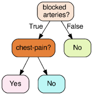
(a) Tree 1

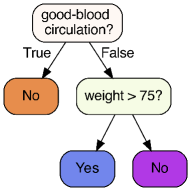
(b) Tree 2

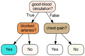
(c) Tree 3

Figure 1: Running example.

Boolean satisfiability (SAT).

The paper assumes the notation and definitions standard in SAT Biere et al. (2021), i.e. the decision problem for propositional logic, which is known to be NP-complete Cook (1971). A propositional formula $\varphi$ is defined over a finite set of Boolean variables $X=\{x_{1},x_{2},\ldots,x_{n}\}$. Formulas are most often represented in conjunctive normal form (CNF). A CNF formula is a conjunction of clauses, a clause is a disjunction of literals, and a literal is a variable ($x_{i}$) or its negation ($\neg{x_{i}}$). Whenever convenient, a formula is viewed as a set of sets of literals. A Boolean interpretation $\mu$ of a formula $\varphi$ is a total mapping of $X$ to $\{0,1\}$ ($0$ corresponds to False and $1$ corresponds to True). Interpretations can be extended to literals, clauses and formulas with the usual semantics; hence we can refer to $\mu(l)$, $\mu(\omega)$, $\mu(\varphi)$, to denote respectively the value of a literal, clause and formula given an interpretation. Given a formula $\varphi$, $\mu$ is a model of $\varphi$ if it makes $\varphi$ True, i.e. $\mu(\phi)=1$. A formula $\varphi$ is satisfiable ($\varphi\operatorname*{\nvDash}\perp$) if it admits a model, otherwise, it is unsatisfiable ($\varphi\operatorname*{\vDash}\perp$). Given two formulas $\varphi$ and $\psi$, we say that $\varphi$ entails $\psi$ (denotes $\varphi\operatorname*{\vDash}\psi$) if all models of $\varphi$ are also models of $\psi$. $\varphi$ and $\psi$ are equivalent (denoted $\varphi\equiv\psi$) if $\varphi\operatorname*{\vDash}\psi$ and $\psi\operatorname*{\vDash}\varphi$.

Abductive explanations.

The paper uses the definition of PI-explanation Shih et al. (2018) (also referred to as abductive explanation (AXp) in Ignatiev et al. (2019)) , based on prime implicants of some decision function (related with the predicted class). Let us consider a given ML model, computing a classification function $\tau$ on feature space $\mathbb{F}$, a point $\mathbf{v}\in\mathbb{F}$, with prediction $c=\tau(\mathbf{v})$, with $\mathbf{v}=(v_{1},\ldots,v_{m})$. A PI-explanation (AXp) is any minimal subset ${\mathcal{X}}\subseteq{\mathcal{F}}$ such that:

$$\forall(\mathbf{x}\in\mathbb{F}).\left[\bigwedge\nolimits_{i\in{{\mathcal{X}}}}(x_{i}=v_{i})\right]\operatorname*{\rightarrow}(\tau(\mathbf{x})=c)$$ (1)

In a similar vein, we consider contrastive explanations (CXps) Miller (2019). A formal definition of contrastive explanation is proposed in recent work Ignatiev et al. (2020).

Contrastive explanations.

Contrastive explanation can be defined as a minimal subset ${\mathcal{Y}}\subseteq{\mathcal{F}}$ that suffice to changing the prediction if features of ${\mathcal{Y}}$ are allowed to take some arbitrary value from their domain. Given $\mathbf{v}=(v_{1},\ldots,v_{m})\in\mathbb{F}$ with $\kappa(\mathbf{v})=c$, a CXp is any minimal subset ${\mathcal{Y}}\subseteq{\mathcal{F}}$ such that,

$$\exists(\mathbf{x}\in\mathbb{F}).\bigwedge\nolimits_{j\in{\mathcal{F}}\setminus{\mathcal{Y}}}(x_{j}=v_{j})\land(\kappa(\mathbf{x})\not=c)$$ (2)

Building on the results of R. Reiter in model-based diagnosis Reiter (1987), Ignatiev et al. (2020) proves a minimal hitting set (MHS) duality relation between AXps and CXps, i.e. AXps are MHSes of CXps and vice-versa.

Example 1.

Consider the binary classifier $\mathfrak{F}$ of the running example. and the instance $(\mathbf{v}=(1,0,1,70),\mathit{Yes})$. If the features good-blood-circulation and weight are allowed to take any possible value from their domain, and the values of the features blocked-arteries and chest-pain are kept to their values in $\mathbf{v}$, then the prediction is still Yes. This means that the features good-blood-circulation and weight can be deemed irrelevant for the prediction of Yes given the other feature values in $\mathbf{v}$. Moreover, by allowing either blocked-arteries or chest-pain to take any value, prediction will change to No. Hence, $\{\textit{blocked-arteries},\textit{chest-pain}\}$ is a subset-minimal set of features sufficient for predicting $\tau(\mathbf{v})=\textit{Yes}$, that is a PI-explanation (AXp). Additionally, setting the value of blocked-arteries to 0 suffices to changing the prediction of $\mathbf{v}$ (i.e. $\tau(0,0,1,70)=\textit{No}$), thus $\{\textit{blocked-arteries}\}$ is a CXp.

3 Complexity of AXps for RFs

Recent work identified classes of classifiers for which one AXp can be computed in polynomial time Audemard et al. (2020); Marques-Silva et al. (2020). These classes of classifiers include those respecting specific criteria of the knowledge compilation map Audemard et al. (2020), but also Naive Bayes and linear classifiers (resp. NBCs and LCs) Marques-Silva et al. (2020). (In the case of NBCs and LCs, enumeration of AXps was shown to be solved with polynomial delay.) One question is thus whether there might exist a polynomial time algorithm for computing one computing AXp of an RF. This section shows that this is unlikely to be the case, by proving that deciding whether a set of features represents an AXp is $\textnormal{D}^{\textnormal{P}}$-complete.

Let $\mathfrak{F}$ be an RF, with classification function $\tau$, and let $\mathbf{v}\in\mathbb{F}$, with prediction $\tau(\mathbf{v})=c\in{\mathcal{K}}$. $\tau$ is parameterized with $c$, to obtain the boolean function $\tau_{c}$, s.t. $\tau_{c}(\mathbf{x})=1$ iff $\tau(\mathbf{x})=c$. A set of literals $I_{\mathbf{v}}$ is associated with each $\mathbf{v}$. Let $\rho$ be a subset of the literals associated with $\mathbf{v}$, i.e. $\rho\subseteq{I_{\mathbf{v}}}$. Hence,

Theorem 1.

For a random forest $\mathfrak{F}$, given an instance $\mathbf{v}$ with prediction $c$, deciding whether a set of literals is an AXp is $\textnormal{D}^{\textnormal{P}}$-complete.

Proof.  Given an instance $\mathbf{v}$ and predicted class $c$, deciding whether a set of literals $\rho$ is an AXp of an RF $\mathfrak{F}$ is clearly in $\textnormal{D}^{\textnormal{P}}$. We need to prove that $\rho\operatorname*{\vDash}\tau_{c}$, which is a problem in coNP. We also need to prove that a set of literals $\rho^{\prime}$, obtained by the removal of any single literal from $\rho$ (and there can be at most $m$ of these), is such that $\rho\operatorname*{\nvDash}\tau_{c}$, a problem in NP. To prove that the problem is hard for $\textnormal{D}^{\textnormal{P}}$, we reduce the problem of computing a prime implicant of a DNF, which is known to be complete for $\textnormal{D}^{\textnormal{P}}$ Umans et al. (2006), to the problem of computing a PI-explanation of an RF $\mathfrak{F}$.
Consider a DNF $\phi=t_{1}\lor\cdots\lor{t_{n}}$, where each term $t_{i}$ is a conjunction of literals defined on a set $X=\{x_{1},\ldots,x_{m}\}$ of boolean variables. Given $\phi$, we construct an RF $\mathfrak{F}$, defined on a set ${\mathcal{F}}$ of $m$ features, where each feature $i$ is associated with an $x_{i}$ element of $X$, and where $D_{i}=\{0,1\}$. Moreover, $\mathfrak{F}$ is such that $\phi(\mathbf{x})=1$ iff $\tau_{1}(\mathbf{x})=1$. $\mathfrak{F}$ is constructed as follows.

1. Associate a decision tree (DT) ${\mathcal{T}}_{i}$ with each term $t_{i}$, such that the assignment satisfying $t_{i}$ yields class 1, and the other assignments yield class 0. Clearly, the size of the DT ${\mathcal{T}}_{i}$ is linear on the size of $t_{i}$, since each literal not taking the value specified by the term will be connected to a terminal node with prediction 0.

2. Create $(n-1)$ additional trees, each having exactly one terminal node and no non-terminal nodes. Moreover, associate class $1$ with the terminal node.

Next, we prove that $\phi(\mathbf{x})=1$ iff $\tau_{1}(\mathbf{x})=1$.

1. Let $\mathbf{x}$ be such that $\phi(\mathbf{x})=1$. Then, there is at least one term $t_{j}$, such that $t_{j}(\mathbf{x})=1$. As a result, the corresponding tree ${\mathcal{T}}_{j}$ in the RF will predict class 1. Hence, at least $n$ trees predict class 1, and at most $n-1$ trees predict class 0. As a result, the predicted class is 1, and so $\tau_{1}(\mathbf{x})=1$.

2. Let $\mathbf{x}$ be such that $\tau_{1}(\mathbf{x})=1$. This means that at least one of the trees associated with the terms $t_{i}$ must predict value 1. Let such tree be ${\mathcal{T}}_{j}$, associated with term $t_{j}$. For this tree to predict class 1, then $t_{j}(\mathbf{x})=1$, and so $\phi(\mathbf{x})=1$.

Now, let $\rho$ be a conjunction of literals defined on $X$. Then, we must have $\rho\operatorname*{\vDash}\phi$ iff $\rho\operatorname*{\vDash}\tau_{1}$. Every model of $\rho$ is also a model of $\phi$, and so it must also be a model of $\tau_{1}$. Conversely, every model of $\rho$ is also a model of $\tau_{1}$, and so it must also be a model of $\phi$. $\Box$

4 AXps for Random Forests

This section outlines the computation of PI-explanations (AXps) for RFs. We first present the algorithm’s organization. The algorithm requires a logical encoding of RFs, which are presented next.

Computing AXps.

A minimal set of features ${\mathcal{X}}\in{\mathcal{F}}$ is an AXp if (1) holds. Clearly, this condition holds iff the following formula is unsatisfiable,

$$\left[\bigwedge\nolimits_{i\in{{\mathcal{X}}}}(x_{i}=v_{i})\right]\land\mathsf{Enc}(\tau(\mathbf{x})\not=c)$$

The previous formula has two components $\langle{\mathcal{H}},{\mathcal{S}}\rangle$. ${\mathcal{H}}$ represents the set of hard clauses, encoding the representation of the ML model and also imposing a constraint on the predicted class, i.e. $\mathsf{Enc}(\tau(\mathbf{x})\not=c)$. ${\mathcal{S}}$ represents the unit (soft) clauses, each capturing a literal $(x_{i}=v_{i})$. Since the clauses in ${\mathcal{S}}$ are soft, they can be dropped (thus allowing $x_{i}$ to take any value) while searching for a minimal subset of ${\mathcal{E}}$ of ${\mathcal{S}}$, such that,

$$\left[\bigwedge\nolimits_{(x_{1}=v_{i})\in{\mathcal{E}}}(x_{i}=v_{i})\right]\land\mathsf{Enc}(\tau(\mathbf{x})\not=c)$$

is unsatisfiable. Our goal is to find a minimal set ${\mathcal{S}}$ such that the pair $\langle{\mathcal{H}},{\mathcal{S}}\rangle$ remains unsatisfiable (where ${\mathcal{S}}$ can be viewed as the background knowledge against which the clauses in ${\mathcal{S}}$ are inconsistent). This corresponds to finding a minimal unsatisfiable subset (MUS) of $\langle{\mathcal{H}},{\mathcal{S}}\rangle$, and so any off-the-shelve MUS extraction algorithm can be used for computing an AXp (as noted in earlier work Ignatiev et al. (2019)).

Clearly, adapting the descibed procedure above of computing one AXp to one that computes a CXp is straightforward. That is, the minimal set ${\mathcal{Y}}$ of ${\mathcal{S}}$ to search is, such that,

$$\left[\bigwedge\nolimits_{(x_{1}=v_{i})\in{\mathcal{S}}\setminus{\mathcal{Y}}}(x_{i}=v_{i})\right]\land\mathsf{Enc}(\tau(\mathbf{x})\not=c)$$

is satisfiable. Further, hitting set duality between AXps and CXps allows to exploit any algorithm for computing MUSes/MCSes to enumerate both kinds of explanations (AXps and CXps). (Recent work Ignatiev et al. (2020); Marques-Silva et al. (2021); Ignatiev and Marques-Silva (2021) exploits the MUS/MCS enumeration algorithm MARCO Liffiton et al. (2016) for enumerating AXps/CXps.)

We detail next how to encode an RF, while requiring some prediction not to hold. We start with a simple encoding of an RF into an SMT formula, and then we detail a purely propositional encoding, which enables the use of SAT solvers.

SMT Encoding.

Several encodings of tree ensemble models, such as Boosted Trees (BTs), have been proposed and they are essentially based on SMT/MILP (see e.g. Chen et al. (2019); Einziger et al. (2019); Ignatiev (2020), etc). Hence, it is natural to follow prior work and propose a straightforward encoding of RFs in SMT. Intuitively, the formulation of RFs into SMT formulas is as follows. We encode every single DT of an RF as a set of implication rules. That is, a DT path (classification rule) is interpreted as a rule of the form $\textit{antecedent}\operatorname*{\rightarrow}\textit{consequent}$ where the antecedent is a conjunction of predicates encoding the non-terminal nodes of the path and the consequent is a predicate representing the class associated with the terminal node of the path. Next, we aggregate the prediction (votes) of the DTs and count the prediction score for each class. This can be expressed by an arithmetic function that calculates the sum of trees predicting the same class. Lastly, a linear inequality checks which class has the largest score.

The implementation of the encoding above resulted in performance results comparable to those of BTs Ignatiev (2020). However, in the case of RFs it is possible to devise a purely propositional encoding, as detailed below.

SAT Encoding.

Our goal is to represent the structure of an RF with a propositional formula. This requires abstracting away what will be shown to be information used by the RF that is unnecessary for finding an AXp. Concretely, and as shown below, the actual values of the features used as literals in the RF need not be considered when computing one AXp. We start by detailing how to encode the nodes of the decision trees in an RF. This is done such that the actual values of the features are abstracted away. Then, we present the encoding of the RF classifier itself, including how the majority voting is represented.

To encode a terminal node of a DT, we proceed as follows. Given a set of classes ${\mathcal{K}}=\{c_{1},c_{2},\ldots,c_{K}\}$, a terminal node $t$ labeled with one class of ${\mathcal{K}}$. Then, we define for each $c_{j}\in{{\mathcal{K}}}$ a variable $l_{j}$ and represent the terminal node $t$ with its corresponding label class $c_{j}$, i.e. $\kappa(t)=c_{j}$.

Moreover, the encoding of a non-terminal node of a DT is organized as follows. Given a feature $j\in{{\mathcal{F}}}$ associated with a non-terminal node $l$, with a domain $\mathbb{D}_{j}$, each outgoing edge of $l$ is represented by a literal $l_{j}$ of the form $x_{j}\bowtie S_{j}$ s.t. $x_{j}\in{{\mathcal{F}}}$ is the variable of feature $j$, $S_{j}\bowtie\mathbb{D}_{j}$ and $\bowtie\>\in{\{=,\subseteq,\in\}}$. Hence we distinguish three cases for encoding $x_{j}\bowtie S_{j}$. For the first case, feature $j$ is binary, and so the literal $l_{j}$ is True if $x_{j}=1$ and False if $x_{j}=0$. For the second case, feature $j$ is categorical, and so we introduce a Boolean variable $z_{i}$ for each value $v_{i}\in\mathbb{D}_{j}$ s.t. $z_{i}=1$ iff $x_{j}=v_{i}$. Assume $S_{j}=\{v_{1},\ldots,v_{n}\}$, then we connect $l_{j}$ to variables $z_{i},i=1,\ldots,n$ as follows: $l_{j}\operatorname*{\leftrightarrow}(z_{1}\vee\ldots\vee z_{n})$ or $\neg l_{j}\operatorname*{\leftrightarrow}(z_{1}\vee\ldots\vee z_{n})$, depending on whether the current edge is going to left or right child-node. Finally, for the third case, feature $j$ is real-valued. Thus, $S_{j}$ is either an interval or a union of intervals. Concretely, we consider all the splitting thresholds of the feature $j$ existing in the RF and we generate (in order) all the possible intervals. Each interval $I_{i}\subseteq\mathbb{D}_{j}$ is denoted by a Boolean variable $z_{i}$. Let us assume $S_{j}=I_{1}\cup\ldots\cup I_{n}$ and $z_{1},\ldots,z_{n}$ are variables associated with $I_{1}\cup\ldots\cup I_{n}$, then we have $l_{j}\operatorname*{\leftrightarrow}(z_{1}\vee\ldots\vee z_{n})$ or $\neg l_{j}\operatorname*{\leftrightarrow}(z_{1}\vee\ldots\vee z_{n})$. Moreover, this encoding can be reduced into a more compact set of constraints (that also improves propagation in the SAT solver). Indeed, if the number of intervals is large the encoding will be as well. Hence, we propose to use auxiliary variables in the encoding. Assume $\mathbb{D}_{j}=I_{1}\cup I_{2}\cup I_{3}$, nodes $l$ and $l^{\prime}$ s.t. $\neg l_{j}\operatorname*{\leftrightarrow}z_{1}$, $\neg l_{j}\operatorname*{\leftrightarrow}(z_{1}\vee z_{2}\vee z_{3})$, $\neg l_{j}^{\prime}\operatorname*{\leftrightarrow}(z_{1}\vee z_{2})$, $l_{j}^{\prime}\operatorname*{\leftrightarrow}z_{3}$, then this can be re-written as: $\neg l_{j}\operatorname*{\leftrightarrow}z_{1}$, $l_{j}\operatorname*{\leftrightarrow}(z_{2}\vee l_{j}^{\prime})$, $\neg l_{j}^{\prime}\operatorname*{\leftrightarrow}(z_{2}\vee\neg l_{j})$, $l_{j}^{\prime}\operatorname*{\leftrightarrow}z_{3}$.

The next step is to encode the RF classifier. Given an RF $\mathfrak{F}$ formed by a set of $M$ DTs, i.e. $\mathfrak{F}=\{{\mathcal{T}}_{1},{\mathcal{T}}_{2},\ldots,{\mathcal{T}}_{M}\}$, and $\tau$ the classification function of $\mathfrak{F}$. For every DT ${\mathcal{T}}_{i}\in\mathfrak{F}$, we encode the set of paths ${\mathcal{R}}_{i}$ of ${\mathcal{T}}_{i}$ as follows:

$$\bigwedge\nolimits_{R_{k}\in{{\mathcal{R}}_{i}}}\left(\left(\bigwedge\nolimits_{l_{j}\in{\mathcal{L}}(R_{k})}l_{j}\right)\operatorname*{\rightarrow}l_{ij}\right)$$ (3)

where $l_{ij}$ is a literal associated with ${\mathcal{T}}_{i}$ in which the voted class is $c_{j}\in{{\mathcal{K}}}$.

For every DT ${\mathcal{T}}_{i}\in\mathfrak{F}$, and every path $R_{k}\in{{\mathcal{R}}_{i}}$, we enforce the condition that exactly one variable $l_{ij}$ is True in ${\mathcal{T}}_{i}$ . This can be expressed as:

$$\left(\bigvee\nolimits_{j=1}^{K}l_{ij}\right)~{}\wedge~{}\sum\nolimits_{j=1}^{K}l_{ij}\leq 1$$ (4)

Finally, for capturing the majority voting used in RFs, we need to express the constraint that the counts (of individual tree selections) for some class $c_{k}\not=c_{j}$ have to be large enough (i.e. greater than, or greater than or equal to) when compared to the counts for class $c_{j}$. We start by showing how cardinality constraints can be used for expressing such constraints. The proposed solution requires the use of $K-1$ cardinality constraints, each comparing the counts of $c_{j}$ with the counts of some other $c_{k}$. Afterwards, we show how to reduce to 2 the number of cardinality constraints used.

Let $c_{j}\in{\mathcal{K}}$ be the predicted class. The index $j$ is relevant and ranges from 1 to $K=|{\mathcal{K}}|$. Moreover, let $1\leq{k}<{j}\leq{K}$. Class $c_{k}$ is selected over class $c_{j}$ if:

$$\small\sum\nolimits_{i=1}^{M}l_{ik}>\sum\nolimits_{i=1}^{M}l_{ij}\Leftrightarrow\sum\nolimits_{i=1}^{M}l_{ik}+\sum\nolimits_{i=1}^{M}\neg{l_{ij}}\geq{M}$$ (5)

Similarly, let $1\leq{j}<{k}\leq{K}$. Class $c_{k}$ is selected over class $c_{j}$ if:

$$\small\sum\nolimits_{i=1}^{M}l_{ik}>\sum\nolimits_{i=1}^{M}l_{ij}\Leftrightarrow\sum\nolimits_{i=1}^{M}l_{ik}+\sum\nolimits_{i=1}^{M}\neg{l_{ij}}\geq{M+1}$$ (6)

(A simple observation is that these constraints can be optimized for the case $|{\mathcal{K}}|=2$.)

It is possible to reduce the number of cardinality constraints as follows. Let us represent (5) and (6), respectively, by $\mathsf{Cmp}_{\prec}(z^{\prec}_{1},\ldots,z^{\prec}_{M})$ and $\mathsf{Cmp}_{\succ}(z^{\succ}_{1},\ldots,z^{\succ}_{M})$. (Observe that the encodings of these constraints differ (due to the different RHSes).) Moreover, in (5) and (6) we replace $(z^{\prec}_{1},\ldots,z^{\prec}_{M})$ and $(z^{\succ}_{1},\ldots,z^{\succ}_{M})$ resp. by $l_{1k},\ldots,l_{Mk}$, for some $k$. The idea is that we will only use two cardinality constraints, one for (5) and one for (6).

Let $p_{k}=1$ iff $k$ is to be compared with $j$. In this case, $\mathsf{Cmp}_{\bowtie}(z^{\bowtie}_{1},\ldots,z^{\bowtie}_{M})$ (where $\bowtie$ is either $\prec$ or $\succ$) is comparing the class counts of $c_{j}$ with the class counts of some $c_{k}$. Let us use the constraint $p_{k}\operatorname*{\rightarrow}(z^{\bowtie}_{i}\leftrightarrow{l_{ik}})$, with $k\in\{1,\ldots,{K}\}\setminus\{j\}$, and $1\leq{i}\leq{M}$. This serves to allow associating the (free) variables $(z^{\bowtie}_{1},\ldots,z^{\bowtie}_{M})$ with some set of literals $(l_{1k},\ldots,l_{Mk})$. Moreover, we also let $p_{0}\operatorname*{\rightarrow}(z^{\bowtie}_{i}\leftrightarrow{1})$ and $p_{j}\operatorname*{\rightarrow}(z^{\bowtie}_{i}\leftrightarrow{1})$, i.e. we allow $p_{0}$ and $p_{j}$ to pick guaranteed winners, and such that $\neg{p_{0}}\lor\neg{p_{j}}$. Essentially, we allow for a guaranteed winner to be picked below $j$ or above $j$, but not both. Clearly, we must pick one $k$, either below or above $j$, to pick a class $c_{k}$, when comparing the counts of $c_{k}$ and $c_{j}$. We do this by picking two winners, one below $j$ and one above $j$, and such that at most one is allowed to be a guaranteed winner (either 0 or $j$):

$$\left(\sum\nolimits_{r=0}^{j-1}p_{r}=1\right)\>\land\>\left(\sum\nolimits_{r=j}^{K}p_{r}=1\right)$$

Observe that, by starting the sum at 0 and $j$, respectively, we allow the picking of one guaranteed winner in each summation, if needed be. To illustrate the described encoding above we consider again the running example.

Example 2.

Consider again the RF $\mathfrak{F}$ of the running example and the instance $\mathbf{v}=(1,0,1,70)$, giving the prediction Yes. Let us define the Boolean variables $x_{1},x_{2}$ and $x_{3}$ associated with the binary features blocked-arteries, good-blood-circulation, chest-pain, resp. and variables $w_{1}$ and $w_{2}$ representing $(\textit{weight}>75)$ and $(\textit{weight}\leq 75)$ resp. and an auxiliary variable $w$. Also, to represent the classes No and Yes, we associate variables denoting the classes for each tree: $\{l_{11},l_{12}\}$ for ${\mathcal{T}}_{1}$, $\{l_{21},l_{22}\}$ for ${\mathcal{T}}_{2}$ and $\{l_{31},l_{32}\}$ for ${\mathcal{T}}_{3}$. Hence, the corresponding set of encoding constraints is: $\{x_{1}\wedge x_{3}\operatorname*{\rightarrow}l_{12}$, $x_{1}\wedge\neg x_{3}\operatorname*{\rightarrow}l_{11}$, $\neg x_{1}\operatorname*{\rightarrow}l_{11}$, $x_{2}\operatorname*{\rightarrow}l_{21}$, $\neg x_{2}\wedge w\operatorname*{\rightarrow}l_{22}$, $\neg x_{2}\wedge\neg w\operatorname*{\rightarrow}l_{21}$, $x_{2}\wedge x_{1}\operatorname*{\rightarrow}l_{32}$, $x_{2}\wedge\neg x_{1}\operatorname*{\rightarrow}l_{31}$, $\neg x_{2}\wedge x_{3}\operatorname*{\rightarrow}l_{32}$, $\neg x_{2}\wedge\neg x_{3}\operatorname*{\rightarrow}l_{31}$, $w\operatorname*{\leftrightarrow}w_{1}$, $\neg w\operatorname*{\leftrightarrow}w_{2}$, $(l_{11}+l_{21}+l_{31})\geq 2$, $x_{1}$, $\neg x_{2}$, $x_{3}$, $w_{2}\}$. Observe that $\{x_{1},\neg x_{2},x_{3},w_{2}\}$ denotes the set of the soft constraints whereas the remaining are the hard constraints.

5 Experimental Results

Dataset	(#F    #C    #I)			RF			CNF		SAT oracle				AXp (RFxpl)				Anchor
				D	#N	%A	#var	#cl	MxS	MxU	#S	#U	Mx	m	avg	%w	avg	%w
ann-thyroid	$(21)$	3	$718$)	4	$2192$	98	$17\,854$	$29\,230$	0.12	0.15	$2$	$18$	0.36	0.05	0.13	$96$	0.32	$4$
appendicitis	$(7)$	2	$43$)	6	$1920$	90	$5181$	$10\,085$	0.02	0.02	$4$	$3$	0.05	0.01	0.03	$100$	0.48	$0$
banknote	$(4)$	2	$138$)	5	$2772$	97	$8068$	$16\,776$	0.01	0.01	$2$	$2$	0.03	0.02	0.02	$100$	0.19	$0$
biodegradation	$(41)$	2	$106$)	5	$4420$	88	$11\,007$	$23\,842$	0.31	1.05	$17$	$22$	2.27	0.04	0.29	$97$	4.07	$3$
ecoli	$(7)$	5	$66$)	5	$3860$	90	$20\,081$	$34\,335$	0.10	0.09	$4$	$2$	0.21	0.05	0.10	$98$	0.38	$2$
glass2	$(9)$	2	$66$)	6	$2966$	90	$7303$	$15\,194$	0.04	0.03	$5$	$4$	0.09	0.02	0.03	$100$	0.61	$0$
heart-c	$(13)$	2	$61$)	5	$3910$	85	$5594$	$11\,963$	0.04	0.02	$6$	$7$	0.07	0.01	0.04	$100$	0.85	$0$
ionosphere	$(34)$	2	$71$)	5	$2096$	87	$7174$	$14\,406$	0.02	0.02	$22$	$11$	0.11	0.02	0.03	$100$	12.43	$0$
iris	$(4)$	3	$60$)	6	$1446$	93	$16\,346$	$25\,603$	0.02	0.01	$2$	$2$	0.05	0.02	0.03	$100$	0.21	$0$
karhunen	$(64)$	10	$200$)	5	$6198$	91	$36\,708$	$70\,224$	1.06	1.41	$35$	$29$	14.64	0.65	2.78	$100$	28.15	$0$
letter	$(16)$	26	$398$)	8	$44\,304$	82	$28\,991$	$68\,148$	1.97	3.31	$8$	$8$	6.91	0.24	1.61	$70$	2.48	$30$
magic	$(10)$	2	$381$)	6	$9840$	84	$29\,530$	$66\,776$	0.51	1.84	$6$	$4$	2.13	0.07	0.14	$99$	0.91	$1$
mofn-3-7-10	$(10)$	2	$128$)	6	$8776$	92	$2926$	$8646$	0.00	0.01	$3$	$7$	0.02	0.01	0.01	$100$	0.29	$0$
new-thyroid	$(5)$	3	$43$)	5	$1766$	100	$17\,443$	$28\,134$	0.03	0.01	$3$	$2$	0.08	0.03	0.05	$100$	0.36	$0$
pendigits	$(16)$	10	$220$)	6	$12\,004$	95	$30\,522$	$59\,922$	2.40	1.32	$10$	$6$	4.11	0.14	0.94	$96$	3.68	$4$
phoneme	$(5)$	2	$540$)	6	$8962$	82	$21\,899$	$49\,840$	0.09	0.07	$3$	$2$	0.22	0.05	0.09	$98$	0.37	$2$
ring	$(20)$	2	$740$)	6	$6188$	89	$19\,114$	$42\,362$	0.27	0.44	$11$	$9$	1.25	0.05	0.25	$92$	7.25	$8$
segmentation	$(19)$	7	$42$)	4	$1966$	90	$21\,288$	$35\,381$	0.11	0.17	$8$	$10$	0.53	0.11	0.31	$100$	4.13	$0$
shuttle	$(9)$	7	$1160$)	3	$1460$	99	$18\,669$	$29\,478$	0.11	0.08	$2$	$7$	0.34	0.05	0.14	$99$	0.42	$1$
sonar	$(60)$	2	$42$)	5	$2614$	88	$9938$	$20\,537$	0.04	0.06	$36$	$24$	0.43	0.04	0.09	$100$	23.02	$0$
spambase	$(57)$	2	$442$)	5	$4614$	92	$13\,055$	$28\,284$	0.07	0.06	$18$	$37$	0.50	0.05	0.11	$100$	6.18	$0$
spectf	$(44)$	2	$54$)	5	$2306$	88	$6707$	$13\,449$	0.07	0.06	$20$	$24$	0.34	0.02	0.07	$100$	8.12	$0$
texture	$(40)$	11	$550$)	5	$5724$	87	$34\,293$	$64\,187$	0.79	0.63	$23$	$17$	3.24	0.19	0.93	$100$	28.13	$0$
threeOf9	$(9)$	2	$103$)	3	$920$	100	$2922$	$4710$	0.00	0.00	$1$	$8$	0.01	0.00	0.01	$100$	0.14	$0$
twonorm	$(20)$	2	$740$)	5	$6266$	94	$21\,198$	$46\,901$	0.08	0.08	$12$	$8$	0.28	0.06	0.10	$100$	5.73	$0$
vowel	$(13)$	11	$198$)	6	$10\,176$	90	$44\,523$	$88\,696$	1.66	2.11	$8$	$5$	4.52	0.15	1.15	$66$	1.67	$34$
waveform-21	$(21)$	3	$500$)	5	$6238$	84	$29\,991$	$57\,515$	0.68	0.54	$10$	$11$	2.27	0.09	0.34	$100$	5.86	$0$
waveform-40	$(40)$	3	$500$)	5	$6232$	83	$30\,438$	$58\,380$	0.50	0.86	$15$	$25$	7.07	0.11	0.88	$100$	11.93	$0$
wdbc	$(30)$	2	$114$)	4	$2028$	96	$7813$	$15\,742$	0.06	0.02	$12$	$18$	0.13	0.03	0.05	$100$	10.56	$0$
wine-recog	$(13)$	3	$72$)	3	$1188$	97	$17\,718$	$28\,421$	0.04	0.04	$5$	$8$	0.13	0.04	0.07	$100$	1.46	$0$
wpbc	$(33)$	2	$78$)	5	$2432$	76	$9078$	$18\,675$	1.00	1.53	$20$	$13$	5.33	0.03	0.65	$79$	3.91	$21$
xd6	$(9)$	2	$172$)	6	$8288$	100	$2922$	$8394$	0.00	0.00	$3$	$6$	0.02	0.01	0.01	$100$	0.57	$0$

Table 1: Performance evaluation of the RF explainability tool (RFxpl), and comparison with Anchor. The table shows results for 32 datasets, i.e. those for which test data accuracy is no less than 76%. Columns #F, #C and #I report, respectively, the number of features, classes and tested instances, in the dataset. Columns D, #N and %A show, respectively, each tree’s max. depth, total number of nodes and test accuracy of an RF classifier. Columns #var and #cl show the number of variables and clauses of a CNF formula encoding an RF classifier along with any instance to analyze. Column MxS (resp. MxU) reports the maximum runtime of a SAT call (UNSAT call, resp.) and column #S (#U, resp.) reports the average number of SAT calls (resp. UNSAT calls) performed to extract an AXp. Column avg (Mx and m, resp.) shows the average (max. and min., resp.) runtime for extracting an explanation. The percentage of won instances is given as %w.

This section assess the performance of our approach to compute PI-explanations (AXps) for RFs and also compares the results with an heuristic explaining model Anchor Ribeiro et al. (2018) The assessment is performed on a selection of 32 publicly available datasets, which originate from UCI Machine Learning Repository UCI (2020) and Penn Machine Learning Benchmarks Olson et al. (2017). Benchmarks comprise binary and multidimensional classification datasets. The number of classes in the benchmark suite varies from 2 to 26. The number of features (resp. data samples) varies from 4 to 64 (106 to 58000, resp.) with the average being 21.9 (resp. 5131.09). When training RF classifiers for the selected datasets, we used 80% of the dataset instances (20% used for test data). For assessing explanation tools, we randomly picked fractions of the dataset, depending on the dataset size. Concretely, for datasets containing, resp., less than 200, 200–999, 1000–9999 and 10000 or more, we randomly picked, resp., 40%, 20%, 10% and 2% of the instances to analyze. The number of trees in each RF is set to 100 while tree depth varies between 3 and 8. (Note that we have tested other values for the number of trees ranging from 30 to 200, and we fixed it to 100 since with 100 trees RFs achieve the best train/test accuracies.) As a result, the accuracy of the trained models varies between 76% to 100%. We use the scikit-learn Pedregosa et al. (2011) ML tool to train RF models. Note that, scikit-learn can only handle binary and ordinal features in the case of RFs. Accordingly, the experiments focus on binary and continuous data and do not include categorical features. In addition, we have overridden the implemented RF learner in sciki-learn so that it reflects the original algorithm described in Breiman (2001) . Furthermore, PySAT Ignatiev et al. (2018) is used to instrument incremental SAT oracle calls.

The experiments are conducted on a MacBook Pro with a Dual-Core Intel Core i5 2.3GHz CPU with 8GByte RAM running macOS Catalina. Table 1 summarizes the results of assessing the performance of our RF explainer tool (RFxpl) on the selected datasets. (The table’s caption also describes the meaning of each column.) As can be observed, and with three exceptions, the average running time of RFxpl is less than 1sec. per instance. In terms of the largest running times, there are a few outliers (this is to be expected since we are solving a $\textnormal{D}^{\textnormal{P}}$-hard problem), and these occur when the number of classes is large. To assess the scalability of RFxpl, we compared RFxpl with the well-known heuristic explainer Anchor Ribeiro et al. (2018). (Clearly, the exercise does not aim to compare the explanation accuracies of Anchor and RFxpl, but only to assess how scalable it is in practice to solve a $\textnormal{D}^{\textnormal{P}}$-complete explainability problem with a propositional encoding and a SAT oracle.) Over all datasets, RFxpl outperforms Anchor on more than 96% of the instances (i.e. 8438 out of 8746). In terms of average running time per instance, RFxpl outperforms Anchor by more than 1 order of magnitude, concretely the average run time of Anchor is 14.22 times larger than the average runtime of RFxpl.

6 Conclusion

This paper proposes a novel approach for explaining random forests. First, the paper shows that it is $\textnormal{D}^{\textnormal{P}}$-complete to decide whether a set of literals is a PI-explanation (AXp) for a random forest. Second, the paper proposes a purely propositional encoding for computing PI-explanations (AXps) of random forests. The experimental results allow demonstrating that the proposed approach not only scales to realistically sized random forests, but it is also significantly more efficient that a state of the art model-agnostic heuristic approach. Given the practical interest in RFs Zhou and Feng (2017), finding AXps represents a promising new application area of SAT solvers.

Two extensions of the work can be envisioned. One extension is to improve further the propositional encoding proposed in this paper, aiming at eliminating the very few cases where heuristic approaches are more efficient. Another extension is to exploit the proposed model (and any of its future improvements) to explain deep random forests Zhou and Feng (2017).

Acknowledgements.

This work is supported by the AI Interdisciplinary Institute ANITI, funded by the French program “Investing for the Future - PIA3” under Grant agreement n^o ANR-19-PI3A-0004.

References

- Asín et al. (2011) R. Asín, R. Nieuwenhuis, A. Oliveras, and E. Rodríguez-Carbonell. Cardinality networks: a theoretical and empirical study. Constraints, 16(2):195–221, 2011.
- Audemard et al. (2020) G. Audemard, F. Koriche, and P. Marquis. On tractable XAI queries based on compiled representations. In KR, pages 838–849, 2020.
- Biere et al. (2021) A. Biere, M. Heule, H. van Maaren, and T. Walsh, editors. Handbook of Satisfiability. IOS Press, 2021.
- Birnbaum and Lozinskii (2003) E. Birnbaum and E. L. Lozinskii. Consistent subsets of inconsistent systems: structure and behaviour. J. Exp. Theor. Artif. Intell., 15(1):25–46, 2003.
- Breiman et al. (1984) L. Breiman, J. H. Friedman, R. A. Olshen, and C. J. Stone. Classification and Regression Trees. Wadsworth, 1984.
- Breiman (2001) L. Breiman. Random forests. Mach. Learn., 45(1):5–32, 2001.
- Chen et al. (2019) H. Chen, H. Zhang, S. Si, Y. Li, D. S. Boning, and C. Hsieh. Robustness verification of tree-based models. In NeurIPS, pages 12317–12328, 2019.
- Cook (1971) S. A. Cook. The complexity of theorem-proving procedures. In STOC, pages 151–158, 1971.
- Darwiche and Hirth (2020) A. Darwiche and A. Hirth. On the reasons behind decisions. In ECAI, pages 712–720, 2020.
- Darwiche and Marquis (2002) A. Darwiche and P. Marquis. A knowledge compilation map. J. Artif. Intell. Res., 17:229–264, 2002.
- Einziger et al. (2019) G. Einziger, M. Goldstein, Y. Sa’ar, and I. Segall. Verifying robustness of gradient boosted models. In AAAI, pages 2446–2453, 2019.
- Feng and Zhou (2018) J. Feng and Z. Zhou. AutoEncoder by forest. In AAAI, pages 2967–2973, 2018.
- Gao and Zhou (2020) W. Gao and Z. Zhou. Towards convergence rate analysis of random forests for classification. In NeurIPS, 2020.
- Guidotti et al. (2019) R. Guidotti, A. Monreale, S. Ruggieri, F. Turini, F. Giannotti, and D. Pedreschi. A survey of methods for explaining black box models. ACM Comput. Surv., 51(5):93:1–93:42, 2019.
- Ignatiev and Marques-Silva (2021) A. Ignatiev and J. Marques-Silva. SAT-based rigorous explanations for decision lists. In SAT, 2021. In Press.
- Ignatiev et al. (2018) A. Ignatiev, A. Morgado, and J. Marques-Silva. PySAT: A Python toolkit for prototyping with SAT oracles. In SAT, pages 428–437, 2018.
- Ignatiev et al. (2019) A. Ignatiev, N. Narodytska, and J. Marques-Silva. Abduction-based explanations for machine learning models. In AAAI, pages 1511–1519, 2019.
- Ignatiev et al. (2020) A. Ignatiev, N. Narodytska, N. Asher, and J. Marques-Silva. From contrastive to abductive explanations and back again. In AI*IA, 2020. (Preliminary version available from https://arxiv.org/abs/2012.11067.).
- Ignatiev (2020) A. Ignatiev. Towards trustable explainable AI. In IJCAI, pages 5154–5158, 2020.
- Li et al. (2018) O. Li, H. Liu, C. Chen, and C. Rudin. Deep learning for case-based reasoning through prototypes: A neural network that explains its predictions. In AAAI, pages 3530–3537, 2018.
- Liffiton et al. (2016) M. H. Liffiton, A. Previti, A. Malik, and J. Marques-Silva. Fast, flexible MUS enumeration. Constraints An Int. J., 21(2):223–250, 2016.
- Lundberg and Lee (2017) S. M. Lundberg and S. Lee. A unified approach to interpreting model predictions. In NeurIPS, pages 4765–4774, 2017.
- Marques-Silva et al. (2020) J. Marques-Silva, T. Gerspacher, M. C. Cooper, A. Ignatiev, and N. Narodytska. Explaining naive bayes and other linear classifiers with polynomial time and delay. In NeurIPS, 2020.
- Marques-Silva et al. (2021) J. Marques-Silva, T. Gerspacher, M. C. Cooper, A. Ignatiev, and N. Narodytska. Explanations for monotonic classifiers. In ICML, 2021. In Press.
- Miller (2019) T. Miller. Explanation in artificial intelligence: Insights from the social sciences. Artif. Intell., 267:1–38, 2019.
- Mollas et al. (2020) I. Mollas, N. Bassiliades, I. P. Vlahavas, and G. Tsoumakas. Lionforests: local interpretation of random forests. In ECAI, volume 2659, pages 17–24, 2020.
- Montavon et al. (2018) G. Montavon, W. Samek, and K. Müller. Methods for interpreting and understanding deep neural networks. Digit. Signal Process., 73:1–15, 2018.
- Olson et al. (2017) R. S. Olson, W. La Cava, P. Orzechowski, R. J. Urbanowicz, and J. H. Moore. Pmlb: a large benchmark suite for machine learning evaluation and comparison. BioData Mining, 10(1):36, 2017.
- Papadimitriou (1994) C. H. Papadimitriou. Computational complexity. Addison-Wesley, 1994.
- Pedregosa et al. (2011) F. Pedregosa, G. Varoquaux, A. Gramfort, V. Michel, B. Thirion, O. Grisel, M. Blondel, P. Prettenhofer, R. Weiss, V. Dubourg, J. Vanderplas, A. Passos, D. Cournapeau, M. Brucher, M. Perrot, and E. Duchesnay. Scikit-learn: Machine learning in Python. Journal of Machine Learning Research, 12:2825–2830, 2011.
- Petkovic et al. (2018) D. Petkovic, R. B. Altman, M. Wong, and A. Vigil. Improving the explainability of random forest classifier - user centered approach. In PSB, pages 204–215, 2018.
- Quinlan (1993) J. R. Quinlan. C4.5: Programs for Machine Learning. Morgan Kaufmann, 1993.
- Reiter (1987) R. Reiter. A theory of diagnosis from first principles. Artif. Intell., 32(1):57–95, 1987.
- Ribeiro et al. (2016) M. T. Ribeiro, S. Singh, and C. Guestrin. ”why should I trust you?”: Explaining the predictions of any classifier. In KDD, pages 1135–1144, 2016.
- Ribeiro et al. (2018) M. T. Ribeiro, S. Singh, and C. Guestrin. Anchors: High-precision model-agnostic explanations. In AAAI, pages 1527–1535, 2018.
- Shih et al. (2018) A. Shih, A. Choi, and A. Darwiche. A symbolic approach to explaining bayesian network classifiers. In IJCAI, pages 5103–5111, 2018.
- Shih et al. (2019) A. Shih, A. Choi, and A. Darwiche. Compiling bayesian network classifiers into decision graphs. In AAAI, pages 7966–7974, 2019.
- UCI (2020) UCI Machine Learning Repository. https://archive.ics.uci.edu/ml, 2020.
- Umans et al. (2006) C. Umans, T. Villa, and A. L. Sangiovanni-Vincentelli. Complexity of two-level logic minimization. IEEE Trans. Comput. Aided Des. Integr. Circuits Syst., 25(7):1230–1246, 2006.
- Yang et al. (2020) L. Yang, X. Wu, Y. Jiang, and Z. Zhou. Multi-label learning with deep forest. In ECAI, volume 325, pages 1634–1641, 2020.
- Zhang et al. (2019) Y. Zhang, J. Zhou, W. Zheng, J. Feng, L. Li, Z. Liu, M. Li, Z. Zhang, C. Chen, X. Li, Y. A. Qi, and Z. Zhou. Distributed deep forest and its application to automatic detection of cash-out fraud. ACM Trans. Intell. Syst. Technol., 10(5):55:1–55:19, 2019.
- Zhao et al. (2019) X. Zhao, Y. Wu, D. L. Lee, and W. Cui. iforest: Interpreting random forests via visual analytics. IEEE Trans. Vis. Comput. Graph., 25(1):407–416, 2019.
- Zhou and Feng (2017) Z. Zhou and J. Feng. Deep forest: Towards an alternative to deep neural networks. In IJCAI, pages 3553–3559, 2017.