Measure Concentration on the OFDM-based Random Access Channel

Abstract

It is well known that CS can boost massive random access protocols. Usually, the protocols operate in some overloaded regime where the sparsity can be exploited. In this paper, we consider a different approach by taking an orthogonal FFT base, subdivide its image into appropriate sub-channels and let each subchannel take only a fraction of the load. To show that this approach can actually achieve the full capacity we provide i) new concentration inequalities, and ii) devise a sparsity capture effect, i.e where the sub-division can be driven such that the activity in each each sub-channel is sparse by design. We show by simulations that the system is scalable resulting in a coarsely 30-fold capacity increase.

1 Introduction

There is meanwhile an unmanageable body of literature on CS for (massive) random access in 5G-6G networks, often termed as compressive random access [1]. A comprehensive overview of competitive approaches for 5G (Rel. 16 upwards) can be found in [2]. Often unnoticed outside the mathematical literature is that the main driving principle of CS is measure concentration: Let $A\in\mathbb{C}^{m\times n}$ be a randomly subsampled FFT matrix such that $\mathbb{E}\left\|Ax\right\|^{2}=\left\|x\right\|^{2}$ for any vector non-random $x\in\mathbb{C}^{n}$, with $|\operatorname{supp}\left(x\right)|\leq k$, then [3, Lemma 12.25]:

$$\mathbb{P}\left(\left|\left\|Ax\right\|^{2}-\left\|x\right\|^{2}\right|>\left(\sqrt{\frac{k}{m}}+\epsilon\right)\left\|x\right\|^{2}\right)$$

$$\leq 2e^{-\frac{\epsilon^{2}m}{2k}\frac{1}{1+2\sqrt{k/m}+\epsilon/3}}$$ (1)

This has been widely exploited for massive random access. Taking this principle forward, in this paper we prove an extended version and show that it can be used to design powerful massive random access systems.

The very recent papers by Choi [4][5] have been brought to our attention and have revived our interest in the problem. In [4] a two-stage, grant-free approach has been presented where in stage one a classical CS-based detector detects the active $n$-dimensional pilots from a large set of size $l$ which is followed in stage two by data transmission using the pilots as spreading sequences. [5] has presented an improved version where the data slots are granted through prior feedback. The throughput is analyzed and simulation show signficant improvement over multi-channel ALOHA. However, missed detection analysis is carried out under overly optimistic assumptions such as ML detection making the results fragile (e.g. the missed detection cannot be independent of $l$ as the results in [5] suggest). Moreover no concrete pilot design (just random) and no frequency diversity is considered which is crucial for the applicability of the design.

We take a different approach here: Instead of overloading $n$ subcarriers with $l>n$ resources we use $n$-point FFT (orthogonal basis) and subdivide the available bandwidth into sub-channelss, and apply hierarchical algorithms for the detection in each of the sub-channels and slots. Then, we show that in a scalable system, i.e. with growing $n$, this approach yields provably the full capacity. The proof is based on two main ingredients. First, a new measure concentration result for a certain family of vectors with common sparsity pattern is proved. Second, we devise a sparsity capture effect, by coarsely bundling (at most) $\log(n)$ frequency resources in an $n$ resource system which are then collaboratively (CS-based) detected. With this scheme, the collision probability in each sub-channel will diminish over $n$. In the simulation section, this is validated for several setting system yielding an 30-fold increase in user capacity.

Notations. The elements of a vector/sequence $x$ are referred to as $(x)_{i}$. The vector $x_{\mathcal{A}}\in\mathbb{C}^{|\mathcal{A}|}$ (matrix $X_{\mathcal{A}}$) is the projection of elements (rows) of the vector $x\in\mathbb{C}^{n}$ (matrix $X$) onto the subspace indexed by $\mathcal{A}\subset[n]$. Depending on the context we also denote by $x_{\mathcal{A}}$ the vector that coincides with $x$ for the elements indexed by $\mathcal{A}$ and is zero otherwise.

2 System Model

Joint detection problems in massive random access, say in 5G uplink, can typically be cast as follows: We allow for a fixed maximum set of $u$ users in a system with a signal space of total dimension $n$, which can possibly be very large, e.g. $2^{14}$ [6]. The $l$-th (time domain) signature $p_{l}\in\mathbb{C}^{n}$ of the $k$-th user is randomly taken from a possibly large pool $\mathcal{P}\subset\mathbb{C}^{n}$ with $r$ ressources. The random mapping $k\hookrightarrow l$ is not one-to-one obviously, so there are collisions, and the access point ”sees” a superposed channel called effective channel of multiple users. While there is no clear way to detect such collisions right away, there is typically some mechanism to detect such collisons later in the collision resolution phase [7]. After the pilot phase the users send data over $t$ slots using the same signature

Let $h_{k}^{\prime}\in\mathbb{C}^{s}$ denote the sampled channel impulse response (CIR) of the $k$-th user, where $s\ll n$ is the length of the cyclic prefix. The $l$-th effective channel is defined through $h_{l}=\sum_{k:k\hookrightarrow l}h_{k},l=1,...,r$. Furthermore, we define the matrix $\text{circ}^{(s)}(p_{l})\in\mathbb{C}^{n\times s}$ to be the circulant matrix with $p_{l}$ in its first column and $s-1$ shifted versions in the remaining columns.

The $k_{s}>0$ non-zero complex-valued channel coefficients are independent normallly distributed with power $\mathbb{E}|(h_{k})_{l}|^{2}=\sigma_{h,l}^{2}$. While $k_{u}>0$ active users have a non-vanishing CIR, inactive users are modeled by $h_{k}^{\prime}=0$. Note that we assume from now on, if not otherwise explicitly stated, that the channel energy is equally distributed within the coefficients, which however does not affect the generality of the results. Hence, we shall set without loss of generality $\sigma_{h}^{2}=1$ so that the Signal-to-Noise Ratio ($\operatorname{SNR}$) becomes

$$\operatorname{SNR}:=\mathbb{E}|h_{0}|^{2}/\sigma^{2}=1/\sigma^{2}.$$

Note, that $\operatorname{SNR}$ does not reflect the true receive $\operatorname{SNR}$ in the system, which is $k_{s}/\sigma^{2}$.

Stacking the CIRs into a single column vector $h=[h_{1}^{T}\ h_{2}^{T}\ldots h_{r}^{T}]^{T}$, the signal received by the base station in Stage-1 is given by:

$$\text{{Stage-1: \ \ }}y_{0}=C(p)h+e_{0},$$

where $C(p)=[\operatorname{circ}^{(s)}(p_{1}),\dots,\operatorname{circ}^{(s)}(p_{r})]\in\mathbb{C}^{n\times rs}$ depends on the stacked signatures $p=[p_{1}^{T}\ p_{2}^{T}\ldots p_{r}^{T}]^{T}$ and $e_{0}\in\mathbb{C}^{n}$ is AWGN with $e_{0}\sim\mathcal{CN}(0,\sigma^{2}I_{n})$.

In Stage-2 each active user takes the same signature and applies data in the remaining $t-1$ slots. Let the data be collected in the vectors $d_{i}\in\mathbb{C}^{u},i=1,...,t-1$. For ease of exposition we assume binary or QPSK data such that $|(d_{i})_{l}|=1$. Define the matrix $D_{i}=\mathrm{diag}(d_{i})\otimes I_{s}$ so that the transmission is given by:

$$\text{{Stage-2: \ \ }}y_{i}=C(p)D_{i}h+e_{i}$$

Notably $h$ and $D_{i}h$ have the same non-zero locations, i.e. same support. To have a reference point for the load of the system we will set $r=u$ without loss of generality (except for the overloading case where $r<u$ in the numerical section). We will refer to the percentage $k_{u}/n$ as the load of the system..

A key idea in compressive random access is that the user identification and channel estimation task needs to be accomplished within a much smaller subspace, compared to the signal space, so that the remaining dimensions can be exploited. The measurements in this subspace are of the form:

$$\left(y_{i}\right)_{\mathcal{B}}=\Phi_{\mathcal{B}}y_{i}=\Phi_{\mathcal{B}}C(p)D_{i}h+\Phi_{\mathcal{B}}e_{i},$$ (2)

where we denote the restriction of some measurement matrix to a set of rows with indices in $\mathcal{B}\subset[n]$ by $\Phi_{\mathcal{B}}$. In practice, randomized (normalized) FFT measurements, $\Phi_{\mathcal{B}}=W_{\mathcal{B}},(W)_{ij}:=n^{-\frac{1}{2}}e^{-\imath 2\pi ij/n}$ for $i,j=0\dots n-1$, are typically implemented. All performance indicators of the scheme strongly depend on the size of the control window $\mathcal{B}$ and its complement $\mathcal{B}^{C}$ where $\mathcal{B}\cup\mathcal{B}^{C}=[n]$. It is desired to keep the size of the observation window $m\leq|\mathcal{B}|$ as small as possible to reduce the control overhead. The unused subcarriers in $\mathcal{B}^{C}$ can then be used to implement further parallel sub-channels for, say, improved user activity detection. In this situation we shall use $\mathcal{B}_{1}=\mathcal{B}$ and $\mathcal{B}_{2},...,\mathcal{B}_{c}\subset\mathcal{B}^{C}$ where $c:=\left\lfloor n/m\right\rfloor>1$ is some (possibly random) integer. Clearly, signature set and even the channels (due to different collisions in the sub-channels) require an additional sub-channel index, i.e. $p^{1},...,p^{c}$ and $h^{1},...,h^{c}$ so that with $y_{i}^{1},...,y_{i}^{c}$ we have:

$$y_{i}^{j}=\Phi_{\mathcal{B}}C(p^{j})D_{i}h^{j}+\Phi_{\mathcal{B}}e_{i}$$ (3)

Finally, we make the assumptions that there is some kind of load estimation and power control, which clearly effects the SNR. We incorporate this into a normalization on $h^{j}$ though for notational convenience such that:

$$\text{{Power-Control: \ \ }}\mathbb{E}\left\|h^{j}\right\|^{2}\leq 1$$

Using tailored signature design, of which the details are omitted due to lack of space, we can derive the following proxy measurement model:

$$y_{i}^{j}=A_{\mathcal{B}_{j}}D_{i}h^{j}+z_{i},$$ (4)

where $A_{\mathcal{B}_{j}}$ can be regarded as a randomized subsampled FFT which is normalized by an additional factor of $\sqrt{n/m}$. Under the assumption that the additive noise $e_{i}$ is Gaussian with variance $\sigma^{2}$, we find that $z\sim\mathcal{CN}(0,\frac{\sigma^{2}}{n}I_{m})$.

3 Detection algorithms

The detection algorithm (channel and data) shall be used in parallel on every sub-channel. For $c>1$ parallel sub-channels, $k_{u}$ splits up to (random) sub-indices $k_{u}^{1},...,k_{u}^{c}$ where $\sum_{j=1}^{c}k_{u}^{j}=k_{u}$. The possibility to reconstruct $\tilde{h}^{j}=\left(h^{j},D_{1}h^{j},...,D_{t-1}h^{j}\right)$ from only a small control window $\mathcal{B}_{j}$ relies on two structural assumptions: The vector $\tilde{h}^{j}$ containing all CIRs has at most $k_{u}^{j}\cdot k_{s}\cdot t$ non-vanishing entries in total. But the hierarchical structure of the non-vanishing entries implies that $\tilde{h}^{j}$ is $(k_{u}^{j},k_{s},t)$-sparse.

The recovery of $(k_{u}^{j},k_{u},t)$-sparse signals from linear measurements, i.e. h-CS, was studied in Ref. [8, 9] following the outline of model-based CS [10]. Therein an efficient algorithm, HiHTP/HiIHT, was proposed and a recovery guarantee based on the generalised restricted isometry property (RIP) constants was proven.

Denote the linear (correlation) detector by: $\Psi_{j}:=({A_{\mathcal{B}_{j}}})^{H}$. Our strategy is to apply hierarchical hard thresholding operator, given by:

$$L_{k_{u},k_{s},t}(x):=\operatorname{supp}\underset{\text{$(k_{u},k_{s},t)$-sparse $y$}}{\operatorname*{arg}\min}\|{x-y}\|,$$ (5)

which computes the support of the best $(k_{u},k_{s},t)$-sparse approximation, sub-channel-wise but jointly on $\Psi_{j}y_{0}^{j},..,\Psi_{j}y_{t-1}^{j}$ to get the support of $h^{j}$, and subsequently to estimate channel and data on this support denoted $(\mathcal{A}_{j}^{\ast})$ where $(\mathcal{A}_{j}^{\ast})_{k}\neq\{\ \}$ (empty set) if and only if:

$$\lVert\left(h_{k}^{j},D_{1}h_{k}^{j},...,D_{t-1}h_{k}^{j}\right)\rVert\geq\sqrt{t\xi}$$

The procedure can be improved by iterate over the residuals of the re-encoded signals as in HiHTP/HiIHT.

4 Performance analysis

4.1 Figures of merit

Missed detection, false alarm. The missed detection probability per user $P_{\text{md}}\left(\xi\right)$ is a key metric for the system. Note that by symmetry the probability of a missed detection is identical for all active users. Since the algorithm works on each sub-channel in parallel, clearly, $P_{\text{md}}\left(\xi\right)$ depends on the load. For $c=1$ the load is simply $k_{u}$. For $c>1$, since an active user can only appear once in any of the sub-channels so that, conditioning on a specific sub-channel selection, the resulting $P_{\text{md}}(\xi)$ is simply the average over the marginal load distribution in this sub-channel. Clearly, this is independent of the sub-channel selection and we could as well just fix a certain sub-channel, say $\mathcal{B}_{1}$, loaded on average with $\bar{k}_{u}:=1+(k_{u}-1)/c$. Eventually, we define the probability that some inactive user is falsely detected as active by $P_{\text{fa}}(\xi)$.

Collision probability. In order to capture the dynamic behavior with parallel $c$ sub-channels, recall that $k_{u}$ out of $u$ devices in total access the random access channel. The average number of non-collided devices $E_{\text{nc}}\left(k_{u}\right)$ is well-known [7] and given by:

$$E_{\text{nc}}\left(k_{u}\right)\geq k_{u}-k_{u}\cdot\frac{k_{u}k_{s}}{c\cdot n}$$ (6)

where the inequality is true for not too large load $k_{u}/u$. Moreover, the left-hand side is valid for any $k_{u}$, i.e. also for $k_{u}>u$, which would violate the sparsity constraint though.

Obviously, for $c=1$, there is always a fraction of at least $k_{u}/u$ devices in collision. For standard CS we have $c\simeq n/k_{u}k_{s}\log({n}/({k}_{u}k_{s}))$, it is easily seen that the collision fraction reduces to approximately $(k_{u}/n)^{2}$ devices. However, we shall see in the following analysis that this does not capture the real behavior of our system which is governed by the sparsity capture effect allowing $c=O(n/\log(n))$ and $r=n/\log^{2}(n)$.

4.2 User detection analysis

Assume (for the moment) some minimum channel energy $h_{\min}$ and no noise. Suppose the energy threshold $\xi$ is chosen as $0<\xi<h_{\min}$ and define $\epsilon=\min\left\{\xi,h_{\min}-\xi\right\}$. We denote the set of all possible index sets of cardinality $k_{s}$ and indices only in the $k$-th block by $\Omega_{k}$. The thresholding operator applied to the linear estimation $\Psi_{j}y_{0}^{j},...,\Psi_{j}y_{t-1}^{j}$ does identify the correct set of users if the following condition holds:

$$\max_{\begin{subarray}{c}k\in\left[u\right]\\ \omega\in\Omega_{k}\end{subarray}}\left|\sum_{l\in\omega}\left|\left\langle h^{j},v_{l}\right\rangle\right|^{2}-\frac{1}{t}\sum_{i\in[t]}\sum_{l\in\omega}\left|\left\langle\Psi_{j}y_{i}^{j},v_{l}\right\rangle\right|^{2}\right|\leq\epsilon.$$

We start with a new concentration result.

Theorem 1

Let $x$ be fixed with $|\operatorname{supp}\left(x\right)|\leq k_{s}k_{u}$. Consider terms of the form $\left\|AD_{0}x\right\|^{2},\left\|AD_{1}x\right\|^{2},...\left\|AD_{t-1}x\right\|^{2}$ where $D_{0}=I_{n},D_{i},i>0,$ are random unitary diagonal matrices. Then:

$$\mathbb{P}\left(\left|\frac{1}{t}\sum_{i\in[t]}\left\|AD_{i}x\right\|^{2}-\left\|x\right\|^{2}\right|>\epsilon\left\|x\right\|^{2}\right)$$

$$\leq\frac{32\log\left(2mk_{s}^{2}k_{u}^{2}\right)+1}{\epsilon^{2}tm}$$

The main difference to the standard approach (1) is that our approach yields a bound which decays with growing $t$. This is in contrast to typical CS bounds. Moreover, a closer inspection yields that it is even true for a statistical support condition of the form $\mathbb{E}_{k_{u}}|\operatorname{supp}\left(x\right)|\leq k_{s}\bar{k}_{u}$.

We will now exploit this result for the misdetection. Since the analysis is independent of user index $k$ and sub-channel $j$ we shall set $k=j=1$. For this let $F^{z}(\xi|x):=\mathbb{P}(\sum_{i}\|(h^{1}+z_{i})_{\mathcal{A}_{1}}\|^{2}\leq\xi|x)$ where $x$ is the (random) sub-channel load $k_{u}^{1}=x$, i.e. the probability that conditioned on $x$ the energy falls below some threshold $\xi$. We let the system scale with $n$ and fix a (non-random sequence) $m_{n}$ from which we get we have $c_{n}=n/m_{n}$ sub-channels.

Theorem 2

Let $\epsilon>0$. Let user 1 be in sub-channel 1 with fixed sub-channel load $x$. There are constants $C_{1},C_{2}$ independent of all parameters:

$$P_{\text{md}}\left(\xi|x\right)\leq F^{z}(\xi+\epsilon|x)$$

$$+C_{1}u\left(\frac{es}{k_{s}}\right)^{k_{s}}\frac{k_{s}^{2}\log\left(2mk_{s}^{2}x^{2}\right)+1}{\epsilon^{2}tm}+C_{2}\left(\frac{\operatorname{SNR}}{n}\right)^{-k_{s}x}$$

Let us interpret the results: First, clearly we see that $P_{\text{md}}\left(\xi|x\right)$ under every load is noise-stable. Second, assume that the sub-channel load $x$ is close to its average $O(k_{u}/c)$ which equals $O(k_{u}/c)=m$ in the fully loaded system $k_{u}=O(n)$. Since $h_{\text{min}}=O(1/x)$ we require that $\epsilon={O(1/x)}$. Hence, if we set $m=x=O(\log(n))$, $u=O(n/x^{2})$ and $t=n$ we see that $P_{\text{md}}\left(\xi|x\right)\rightarrow 0$ (fixed $k_{s}$). Hence, for the result to hold we need to show that each sub-channel load is indeed not higher than $O(\log\left(n\right))$ with high probability so that in each sub-channel the collision turns to zero.

4.3 User collision analysis

The sparsity capture effect works as follows: We can think of the baseline system as distributing $k_{u}$ users for the $n$ resources (in the frequency domain) which leads to collisions. Now suppose we bundle $y\left(x\right)$ resources together, call it the sub-channel, and possess a mechanism that can handle $x$ users with high probability (i.e., by our hierarchical CS sensing algorithm). The resulting number of sub-channels as $c\left(x\right)=n/y\left(x\right)$. Clearly, such sub-channel load is binomial-distributed. By applying the Poisson approximation (which is exact for large $n$) and the union bound, the following result shows indeed that the number of subchannels $c\left(x\right)$ grows fast enough to ensure that the effective load in the sub-channels remains sparse with overwhelming probability.

Theorem 3

(sparsity capture effect) If $y(x)\leq x$ then:

$$\mathbb{P}\left(\{x\geq k_{u}^{1}\}\right)\leq\frac{n\left(k_{u}-x\right)}{x\sqrt{2\pi x}}e^{-\left(1-\frac{k_{u}}{n}\right)^{2}x}$$

Let us again interpret the result: If the number of measurements equals $m=O(\log(n))$, then the probability that $x\geq O(((1-\frac{k_{u}}{n})^{-2}\log n))$ or more users are in some specific sub-channel turns to zero for any load $k_{u}/n<1$ as $n$ grows. Hence sub-channel load $x$ concentrates around $O(\log(n))\$ and probability of collision in each sub-channel turns to zero with $n$ as well, obviously, thus completing our analysis. We will validate now our results in the next section.

5 Evaluations and Simulations

Parallel sub-channels are created by randomly partitioning the $n$-dimensional image space into blocks of length $m$, leading to $c=n/m$ sub-channels. For each sub-channel $j=1,\ldots,c$, a vector $x^{j}\in\mathbb{C}^{n}$ is divided into $u$ blocks, each of length $s$, such that $n=us$. If a user chooses resource block $k\in[u]$, block $x_{k}$ is filled with the $k$th user’s $k_{s}$-sparse signature. We allow for $k_{u}^{j}=\bar{k}_{u}$ users per sub-channel. Each user is also encoding data into diagonal matrices $D_{i}$, $i=2,\ldots,t$ containing entries of modulus 1. Hence, at the BS data blocks $y_{i}^{j}=A_{j}D_{i}x^{j}\in\mathbb{C}^{m}$ for $j=1,\ldots,c,i=0,\ldots,t$ are received, forming the observation $y\in\mathbb{C}^{c\times m\times t}$. Here, $A_{j}$ is a matrix consisting of $m$ rows of a $n\times n$ DFT matrix, corresponding to the frequencies allocated to sub-channel $j$.

User detection is performed by one step of Hi-IHT [9]. The number $\bar{k}_{u}$ of users per sub-channel is chosen such that the probability of 2 or more users trying to access the same resource block is below a preset probability $0<p_{u}<1$, i.e. the largest $k\in\mathbb{N}$ such that

$$\prod\limits_{i=1}^{k}\left(1-\frac{i}{n}\right)\geq 1-p_{u}.$$ (7)

The left hand side of inequality (7) is the probability that each of $k$ indices out of $[u]$ selected uniformly at random are unique. Hence, on average the total number of supported users is given by $(1-p_{u})\cdot\bar{k}_{u}\cdot c\cdot(1-P_{md})$. In our simulations we considered blocks of length $s=8$ with an in-block sparsity $k_{s}=4$. Then, $\bar{k}_{u}$ was selected such that $p_{u}\geq 0.1$. We set $t=100$ and $m=2^{\lfloor\log_{2}(\bar{k}_{u}\cdot k_{s})\rfloor}$, which resulted in detection rates close to 1 in noise-free simulations. The number of supported users in this setting for $n=2^{10},\ldots,2^{13}$ can be observed in fig 1, which shows that the system also performs well under noise. With a SNR $\geq-10$dB the system performance is virtually indistinguishable from the noise free case. To give concrete numbers: Assuming 60kHz subcarrier spacing and FFT size 4096 the system reliably detects 450000 devices per second with good load, e.g. estimated 100kByte for rate $1/4$ code.

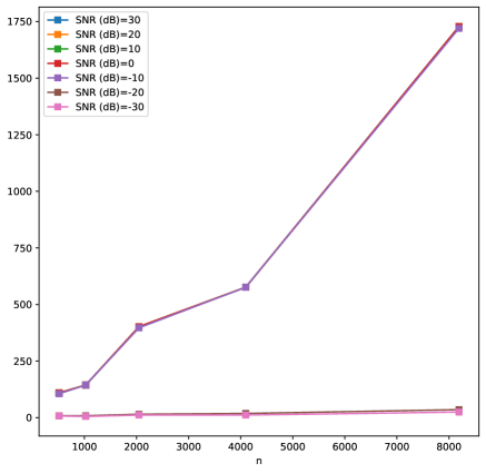
Fig. 1: Average number of supported users (100 Monte-Carlo trials)

6 Conclusion

Exploiting a new measure concentration inequality, we designed a massive random access scheme based on hierarchical compressed sensing, conducted theoretical performance analysis and demonstrated its feasibility by numerical simulations. The proposed scheme promises huge gains in terms of throughput and number of supported users.

References

- [1] G. Wunder, H. Boche, T. Strohmer, and P. Jung. Sparse Signal Processing Concepts for Efficient 5G System Design. IEEE ACCESS, December 2015.
- [2] C. Bockermann, N. Patras, G. Wunder, and et al. Towards Massive Connectivity Support for Scalable mMTC Communications in 5G networks. IEEE ACCESS, May 2018.
- [3] Simon Foucart and Holger Rauhut. A mathematical introduction to Compressed Sensing. Birkhäuser, 2013.
- [4] J. Choi. Stability and throughput of random access with cs-based mud for mtc. IEEE Transactions on Vehicular Technology, 67(3):2607–2616, 2018.
- [5] J. Choi. On throughput of compressive random access for one short message delivery in iot. IEEE Internet of Things Journal, 7(4):3499–3508, 2020.
- [6] Gerhard Wunder, Peter Jung, and Mohammed Ramadan. Compressive Random Access Using A Common Overloaded Control Channel. In IEEE Global Communications Conference (Globecom’14) – Workshop on 5G & Beyond, San Diego, USA, December 2015.
- [7] M. I. Hossain, A. Azari, and J. Zander. Dera: Augmented random access for cellular networks with dense h2h-mtc mixed traffic. In 2016 IEEE Globecom Workshops (GC Wkshps), pages 1–7, Dec 2016.
- [8] I. Roth, M. Kliesch, A. Flinth, G. Wunder, and J. Eisert. Reliable recovery of hierarchically sparse signals for Gaussian and Kronecker product measurements. IEEE Transactions on Signal Processing, 68:4002–4016, 2020.
- [9] Gerhard Wunder, Stelios Stefanatos, Axel Flinth, Ingo Roth, and Giuseppe Caire. Low-overhead hierarchically-sparse channel estimation for multiuser wideband massive mimo. IEEE Transactions on Wireless Communications, 18(4):2186–2199, 2019.
- [10] R. G. Baraniuk, V. Cevher, M. F. Duarte, and C. Hegde. Model-based compressive sensing. IEEE Trans. Inf. Th., 56(4):1982–2001, April 2010.