Quantum metrology with one auxiliary particle in a correlated bath
and its quantum simulation

Abstract

In realistic metrology, entangled probes are more sensitive to noise, especially for a correlated environment. The precision of parameter estimation with entangled probes is even lower than that of the unentangled ones in a correlated environment. In this paper, we propose a measurement scheme with only one auxiliary qubit, which can selectively offset the impact of environmental noise under this situation. We analyse the estimation precision of our scheme and find out that it approaches the Heisenberg limit when prepared in a proper auxiliary state. We further discuss employing auxiliary states to improve the precision of measurement in other environment models such as a partially-correlated environment. In order to verify our scheme, we apply a recently-developed quantum algorithm to simulate the quantum dynamics of our proposal and show that it outperform the other proposals with less resources.

I introduction

Quantum metrology employs quantum entanglement and coherence to achieve an ultra-high precision for the estimation of an unknown parameter (Giovannetti et al., 2011; Degen et al., 2017). It has become an indispensable element of satellite navigation, aerospace measurement and control, mobile phone and computer chip processing. This opens a broad range of valuable applications of quantum mechanics, in addition to quantum information processing (Nielsen and Chuang, 2000), photosynthetic exciton energy transfer (Lambert et al., 2013; Ai et al., 2013a), avian magnetoreception (Cai et al., 2012; Yang et al., 2012; Lambert et al., 2013; Cai and Plenio, 2013) and quantum metamaterial (Oktel and Müstecaplıoğlu, 2004; Thommen and Mandel, 2006; Kästel et al., 2007; Zhao et al., 2020). As a result of the central-limit theorem, the estimated precision of an unknown quantity critically depends on the number of resources available for the measurement. One of the primary goals of quantum metrology is to enhance the precision of resolution with limited resources. An enhanced resolution can be achieved if quantum entanglement is used to correlate the probes before making them interact with the system to be measured (Braunstein, 1992; Giovannetti et al., 2004). Taking advantage of $n$ entangled quantum probes, one can attain the Heisenberg limit (HL) which scales as $n^{-1}$, being the ultimate limit in precision set by quantum mechanics. And this result has been demonstrated experimentally (Leibfried et al., 2004; Roos et al., 2006). On the contrary, when using unentangled probes, one can only reach the standard quantum limit (SQL) which scales as $n^{-1/2}$. Obviously, the use of entanglement can significantly enhance the precision when $n$ is large.

In realistic scenario for experiments, quantum probes are inevitably affected by noise. The achievable precision decreases due to the decoherence. As known to all, the quantum dynamics of open quantum systems are usually classified into Markovian and non-Markovian Breuer et al. (2016); de Vega and Alonso (2017); Li et al. (2018); Breuer et al. (2009); Liu et al. (2011); Rivas et al. (2010). When the system-bath couplings are relatively large, or the number of degrees of freedom in the environment is not sufficiently large, e.g. natural photosynthetic complexes and NV centers in diamond, the open quantum systems are subject to non-Markovian quantum dynamics (Lambert et al., 2013; Childress et al., 2006). Using entangled probes in a non-Markovian quantum dynamics allows for a higher measurement precision than that in a Markovian quantum dynamics, which scales as $n^{-3/4}$ (Chin et al., 2012). On the other hand, when particles interact with a correlated environment, e.g. nuclear spins in a molecule, the decoherence rate per particle will increase linearly with the number of particles, i.e., superdecoherence (Kattemölle and van Wezel, 2020). In this regime, utilizing entangled probes will no longer outperform unentangled ones no matter the open quantum dynamics is Markovian or non-Markovian.

In order to overcome decoherence in an uncorrelated bath, logical states are introduced to establish decoherence-free subspace (Dorner, 2012; Yousefjani et al., 2017; Song et al., 2016). However, since $\mathit{N}$ logical qubits require $n=2N$ physical qubits, it doubles the number of valuable resources used per experiment. In order to effectively reduce the usage of resources, here we propose a measurement scheme with only one auxiliary qubit in a correlated bath. Using such a well-designed auxiliary particle in quantum metrology can selectively offset the impact of noise in a correlated environment. Comparing with previous proposals, we show that although we use less resources, we can still approach the HL when preparing proper auxiliary states.

On the other hand, although the theoretical scheme utilizing entanglement in a non-Markovian environment is appealing, it might be difficult to experimentally verify it since it critically requires the homogeneity of the qubits. For example, for NV centers in diamond, different spins manifest different Zeeman energies and decoherence rates in the same environment due to the inhomogeneous gyromagnetic ratios. Recently, based on the bath-engineering technique (Soare et al., 2014a, b) and the gradient ascent pulse engineering (GRAPE) algorithm (Khaneja et al., 2005; Li et al., 2017a), we theoretically proposed and experimentally demonstrated that the open quantum dynamics with an arbitrary Hamiltonian and spectral density can be exactly and efficiently simulated Wang et al. (2018); Zhang et al. (2021). Thus, based on this algorithm, we show how to verify that our scheme can make the estimation precision achieve the HL in a quantum simulation experiment (Buluta and Nori, 2009; Georgescu et al., 2014).

This paper is organized as follows: Our measurement scheme and its quantum dynamics for quantum metrology in a correlated bath are introduced in the next section. Specifically, we offer an example of magnetic-field sensing utilizing our measurement scheme. Then, in Sec. III, we apply a recently-developed quantum algorithm to simulate our measurement scheme with an auxiliary qubit and show that it can approach the HL. In Appendix, we give a brief description for the open quantum dynamics of $n$ qubits in a correlated bath and an uncorrelated bath, respectively.

II Model and Dynamics

II.1 Quantum Metrology under Superdecoherence

In quantum metrology, using entangled probes can obtain an increase in precision when assuming a fully-coherent evolution, while in realistic scenario, there is always decoherence caused by environmental noise. The optimal precision with entangled probes under decoherence was first analyzed in Markovian environment (Huelga et al., 1997), and further discussed in non-Markovian environment (Chin et al., 2012). The best resolution in the estimation was obtained with a given number of particles $n$ and a total duration of experiment $T$, i.e., $nT/t$ being the actual number of experiment. The entangled probes are prepared in an $n$-qubit GHZ state $(|0\rangle^{\otimes N}+|1\rangle^{\otimes N})/\sqrt{2}$, and then evolve freely for a duration $t$. In the ideal case, we have $(|0\rangle^{\otimes N}+\exp(-in\phi t)|1\rangle^{\otimes N})/\sqrt{2}$, where $\phi$ is the parameter to be estimated. However, in the presence of dephasing noise, the final state becomes $\{|0\rangle^{\otimes N}+\exp[-in\phi t-\Gamma_{n}(t)]|1\rangle^{\otimes N}\}/\sqrt{2}$, with $\Gamma_{n}\left(t\right)=\int_{0}^{t}d\tau\gamma_{n}(\tau)$, and $\gamma_{n}(t)$ being the dephasing rate of $n$ qubits. After a $\pi/2$ pulse, the probability of finding these probes in the initial state reads

$$P=\frac{1}{2}\left[1+\cos(n\phi t)e^{-\Gamma_{n}(t)}\right].$$ (1)

The uncertainty of the measurement can be calculated as

$$\delta\phi^{2}=\frac{1}{\left(nT/t\right)F\left(\phi\right)},$$ (2)

where the Fisher information (Breuer and Petruccione, 2002; Liu et al., 2017) is

$$F(\phi)\equiv\frac{1}{P(1-P)}\left(\frac{\partial P}{\partial\phi}\right)^{2}=\frac{t^{2}\sin^{2}(\phi t)e^{-2\Gamma_{n}(t)}}{1-\cos^{2}(\phi t)e^{-2\Gamma_{n}(t)}}.$$ (3)

When the entangled probes are in uncorrelated environment, we can obtain $\Gamma_{n}(t)=n\int_{0}^{t}d\tau\gamma(\tau)=n\Gamma(t)$, where $\gamma(t)$ and $\Gamma(t)$ are respectively the dephasing rate and decoherence factor for a single qubit. Thus, the uncertainty is explicitly written as (Huelga et al., 1997; Chin et al., 2012)

$$\delta\phi^{2}=\frac{1-\cos^{2}\left(\phi t\right)e^{-2n\Gamma\left(t\right)}}{nTt\sin^{2}\left(\phi t\right)e^{-2n\Gamma\left(t\right)}}.$$ (4)

In order to attain the best precision, it is necessary to optimize this expression of uncertainty against the duration of each single measurement $t$. The best interrogation time satisfies $\phi t_{e}=k\pi/2$ with odd $k$ and $2nt\frac{d\Gamma(t)}{dt}\mid_{t=t_{e}}=1$ (Chin et al., 2012), and thus yields

$$\delta\phi^{2}\mid_{e}=\frac{1}{n^{2}Tt_{e}}e^{2n\Gamma\left(t_{e}\right)},$$ (5)

where the subscript $e$ indicates that the entangled probes are used.

When the entangled probes are in a correlated environment, the superdecoherence of the probes will modify the probability as

$$P=\frac{1}{2}\left[1+\cos\left(n\phi t\right)e^{-n^{2}\Gamma\left(t\right)}\right].$$ (6)

The uncertainty of parameter $\phi$ reads

$$\delta\phi^{2}|_{e}=\frac{1-\cos^{2}\left(n\phi t\right)e^{-2n^{2}\Gamma\left(t\right)}}{nTt\sin^{2}\left(n\phi t\right)e^{-2n^{2}\Gamma\left(t\right)}}.$$ (7)

By minimizing $\delta\phi^{2}|_{e}$, i.e., requiring that $\phi t_{e}=k\pi/2$ with odd $k$ and $2n^{2}t\frac{d\Gamma\left(t\right)}{dt}\mid_{t=t_{e}}=1$, we have

$$\delta\phi^{2}|_{e}=\frac{1}{n^{2}Tt_{e}}e^{2n^{2}\Gamma\left(t_{e}\right)}.$$ (8)

When utilizing unentangled probes, the uncertainty of parameter is $\delta\phi^{2}\mid_{u}=\frac{1}{nTt_{u}}\exp[2\Gamma(t_{e})]$, and the best interrogation time is given by $\phi t_{u}=k\pi/2$ with odd $k$ and $2t\frac{d\Gamma(t)}{dt}\mid_{t=t_{u}}=1$ (Chin et al., 2012). Following Ref. (Chin et al., 2012), we define

$$r=\frac{\delta\phi|_{u}}{\delta\phi|_{e}},$$ (9)

where $\left|\delta\phi\right|_{e}$ and $\left|\delta\phi\right|_{u}$ are the standard deviation of the estimated parameter $\phi$ when using entangled and unentangled probes, respectively. Here, $r$ characterizes the improved precision of measurement for using entangled probes instead of unentangled ones. For entangled probes in an uncorrelated environment, we obtain $r^{2}=n(t_{e}/t_{u})\exp[2\Gamma(t_{u})-2n\Gamma(t_{e})]$, while for entangled probes in a correlated environment, we have $r^{2}=n(t_{e}/t_{u})\exp[2\Gamma(t_{u})-2n^{2}\Gamma(t_{e})]$. Obviously, $r$ changes along with the dependence of function $\Gamma(t)$ on time (Chin et al., 2012), i.e., the dynamics of decoherence. For example, $\Gamma(t)\propto t$ corresponds to the Markovian dephasing dynamics. When $\Gamma(t)$ has a quadratic behavior, i.e., $\Gamma(t)\propto t^{2}$, it is the non-Markovian dephasing dynamics, which is actually the quantum Zeno dynamics Yousefjani et al. (2017); Ai et al. (2010, 2013b); Harrington et al. (2017). Hereafter, we just follow the terminology in Ref. (Chin et al., 2012). In Tab. 1, we analyze the relative resolution of the parameter $r$ in different situations, i.e., Markovian vs non-Markovian dynamics and correlated vs uncorrelated environment. We can learn from Tab. 1 that using entangled probes can not improve the precision in the presence of superdecoherence because $r\leq 1$ for $n\geq 2$.

Table 1: The relative parameter resolution $r$ varies with different dephasing dynamics

	uncorrelated environment	correlated environment
Markovian	$r=1$	$r=n^{-1/2}$
non-Markovian	$r=n^{1/2}$	$r=1$

II.2 Quantum Metrology Using an Auxiliary Particle

As shown in the pervious section, on account of superdecoherence, the best precision with entangled probes will no longer be superior to that with unentangled ones. Previous works (Dorner, 2012; Yousefjani et al., 2017) introduced logical states which are decoherence-free to improve the precision at the cost of doubled resources used per experiment. In this section, we present a measurement scheme with auxiliary states, only one auxiliary qubit being used per experiment. When we prepare a properly-designed auxiliary qubit, the precision of parameter estimation can approach the HL.

As illustrated in Fig. 1, we initially prepare an $(N+1)$-qubit entangled state with $N$ being the number of working qubits, i.e.,

$$|\Psi(0)\rangle=\frac{1}{\sqrt{2}}\left(|1\rangle_{a}|0\rangle^{\otimes N}+|0\rangle_{a}|1\rangle^{\otimes N}\right),$$ (10)

where the subscript $a$ indicates the auxiliary qubit.

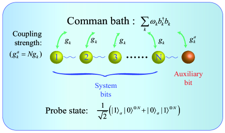
Figure 1: Schematic for $N$-qubits and 1 auxiliary qubit in a correlated bath. An $(N+1)$-qubit entangled system, initially at $|\Psi(0)\rangle=(|1\rangle_{a}|0\rangle^{\otimes N}+|0\rangle_{a}|1\rangle^{\otimes N})/\sqrt{2}$, interacts with a correlated bath. The coupling constants between the qubits and the $k$th mode of the bath satisfy $g_{k}^{a}=Ng_{k}$.

The total system is governed by the Hamiltonian $H=H_{\textrm{S}}+H_{\textrm{B}}+H_{\textrm{int}}$, $H_{\textrm{S}}$ and $H_{\textrm{B}}$ being the Hamiltonian of probe and bath, $H_{\textrm{int}}$ being the interaction Hamiltonian

$$H = \frac{1}{2}\Omega_{0}\sum_{i=1}^{N}\sigma_{z}^{(i)}+\frac{1}{2}\omega_{a}\sigma_{z}^{a}+\sum_{k}\omega_{k}b_{k}^{\dagger}b_{k}$$ (11)

$$+\sum_{k}\sum_{i=1}^{N}(g_{k}^{(i)}\sigma_{z}^{(i)}+g_{k}^{a}\sigma_{z}^{a})(b_{k}^{\dagger}+b_{k}),$$

where $\omega_{a}$ is the frequency of the auxiliary qubit, we assume identical frequency $\Omega_{0}$ for the $N$ working qubits, $\sigma_{z}^{(i)}$ and $\sigma_{z}^{a}$ are the Pauli operators of the working and auxiliary qubits, respectively, $g_{k}$ ($g_{k}^{a}$) denotes the coupling constant between the working (auxiliary) qubit and the $k$th mode of the environment, $b_{k}^{\dagger}$ is the creation operator of the harmonic oscillator with frequency $\omega_{k}$.

According to Eq. (A), the quantum dynamics of the reduced density matrix of the total system including the working and auxiliary qubits is described by the quantum master equation

$$\dot{\rho} = i[\rho,H_{\textrm{S}}+H_{\textrm{LS}}]$$ (12)

$$+\frac{1}{2}[\sum_{i,j=1}^{N}C_{ij}(0,t)(\sigma_{z}^{(j)}\rho\sigma_{z}^{(i)}-\frac{1}{2}\{\sigma_{z}^{(i)}\sigma_{z}^{(j)},\rho\})$$

$$+\sum_{i=1}^{N}C_{ia}(0,t)(\sigma_{z}^{a}\rho\sigma_{z}^{(i)}-\frac{1}{2}\{\sigma_{z}^{(i)}\sigma_{z}^{a},\rho\})$$

$$+\sum_{i=1}^{N}C_{ai}(0,t)(\sigma_{z}^{(i)}\rho\sigma_{z}^{a}-\frac{1}{2}\{\sigma_{z}^{a}\sigma_{z}^{(i)},\rho\})$$

$$+C_{aa}(0,t)(\sigma_{z}^{a}\rho\sigma_{z}^{a}-\rho)],$$

where the time correlation functions are

$$C_{AB}(\omega,t)=2\sum_{k}g_{k}^{A}g_{k}^{B}\left[2\overline{n}(\omega_{k},T)+1\right]\frac{\sin\omega_{k}t}{\omega_{k}}|_{\omega_{k}=\omega}$$ (13)

for $A,B=i,j,a$ with $\overline{n}(\omega_{k},T)$ being the Bose-Einstein distribution at temperature $T$, $\{A,\rho\}=A\rho+\rho A$ is the anti-commutator,

$$H_{\textrm{LS}} = \sum_{i,j=1}^{N}F_{ij}(0,t)\sigma_{z}^{(i)}\sigma_{z}^{(j)}+\sum_{i=1}^{N}F_{ia}(0,t)\sigma_{z}^{(i)}\sigma_{z}^{a}$$ (14)

$$+\sum_{i=1}^{N}F_{ai}(0,t)\sigma_{z}^{a}\sigma_{z}^{(i)}+F_{aa}(0,t)\mathbb{I},$$

is the Hamiltonian with the Lamb shift

$$F_{AB}(\omega,t)=\sum_{k}g_{k}^{A}g_{k}^{B}\frac{\cos\omega_{k}t-1}{\omega_{k}}|_{\omega_{k}=\omega}$$ (15)

for $A,B=i,j,a$, $\mathbb{I}$ is the identity operator.

II.2.1 Correlated Environment

Suppose entangled probes are physically close, i.e., $g_{k}^{(j)}=g_{k}$ for $j=1,2,\cdots N$. They may suffer from superdecoherence with the time correlation function $C_{ij}(0,t)=\gamma(t)$ for $i,j=1,2,\cdots N$. As illustrated in Fig. 1, in our measurement scheme, we prepare a proper auxiliary qubit, whose coupling constant with the $k$th mode in the bath reads $g_{k}^{a}=Ng_{k}$. Thus, we have $C_{ia}(0,t)=C_{ai}(0,t)=N\gamma(t)$, and $C_{aa}=N^{2}\gamma(t)$. Equation (12) is rewritten as

$$\dot{\rho} = i[\rho,H_{\textrm{S}}+H_{\textrm{LS}}]$$ (16)

$$+\frac{1}{2}[\sum_{i,j=1}^{N}\gamma(t)(\sigma_{z}^{(j)}\rho\sigma_{z}^{(i)}-\frac{1}{2}\{\sigma_{z}^{i}\sigma_{z}^{(j)},\rho\})$$

$$+N\sum_{i=1}^{N}\gamma(t)(\sigma_{z}^{a}\rho\sigma_{z}^{(i)}-\frac{1}{2}\{\sigma_{z}^{(i)}\sigma_{z}^{a},\rho\})$$

$$+N\sum_{i=1}^{N}\gamma(t)(\sigma_{z}^{(i)}\rho\sigma_{z}^{a}-\frac{1}{2}\{\sigma_{z}^{a}\sigma_{z}^{(i)},\rho\})$$

$$+N^{2}\gamma(t)(\sigma_{z}^{a}\rho\sigma_{z}^{a}-\rho)].$$

For simplicity, we denote $|1\rangle\equiv|0_{a}\rangle|1\rangle^{\otimes N}$ and $|2\rangle\equiv|1_{a}\rangle|0\rangle^{\otimes N}$. The diagonal terms of the density matrix are constant in time, while the off-diagonal term is given by

$$\rho_{12}(t)=e^{-i\left(N\Omega_{0}-\omega_{a}\right)t}\rho_{12}(0).$$ (17)

As in the conventional quantum metrology scheme, after a free evolution for a time interval $t$ and a $\pi/2$ pulse, the probability of finding the probes in the initial state reads

$$P=\frac{1}{2}[1+\cos(N\Omega_{0}-\omega_{a})t].$$ (18)

We investigate Eq. (18) for different decoherence dynamics in Fig. 2. According to Eq. (8), the entangled probes have a higher precision when experiencing a longer evolution time $t_{e}$. Since the best interrogation time for the correlated bath is much shorter than that for the uncorrelated bath, the precision for the former is much worse. However, in our scheme, the HL can be recovered because the effects of the noises on the working qubits have been effectively canceled due to the auxiliary qubit. We further compare the case in non-Markovian dynamics with the one in Markovian dynamics. The best interrogation times are longer for the former, which is consistent with the prediction in Ref. Chin et al. (2012).

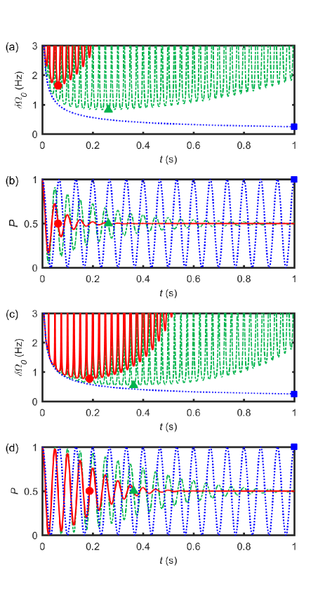
Figure 2: The uncertainty of the measurement $\delta\Omega_{0}$ for (a) a Markovian dephasing dynamics with $\Gamma(t)=\alpha t$, (c) a non-Markovian dynamics with $\Gamma(t)=\beta t^{2}$. Equation (18) for (b) a Markovian dephasing dynamics, (d) a non-Markovian dynamics. The dashed green line indicates the uncorrelated decoherence. The solid red line indicates the superdecoherence in correlated environment. And the dotted blue line indicates our scheme. The green triangle, red circle and blue square show the best interrogation time for uncorrelated decoherence, superdecoherence and our scheme, respectively. We use the following parameters, $n=4$, $\Omega_{0}=2\pi\times 5$ Hz, $\alpha=1$ s^-1, $\beta=1$ s^-2, $T=1$ s.

According to Eq. (8), the best resolution in the estimation satisfies $(N\Omega_{0}-\omega_{a})t_{e}=k\pi/2$ with odd $k$. The uncertainty in our scheme reads

$$\delta\omega_{0}^{2}\mid_{e}=\frac{1}{N^{2}Tt_{e}}=\frac{1}{\left(n-1\right)^{2}Tt_{e}}\propto\frac{1}{\left(n-1\right)^{2}},$$ (19)

where $n=N+1$. $N$ is smaller than $n$ due to the auxiliary qubit.

For unentangled probes, each probe needs a properly-designed auxiliary qubit to cancel the effects of the noises on it. The uncertainty of the measurement is

$$\delta\omega_{0}^{2}\mid_{u}=\frac{1}{N^{\prime}Tt_{u}}=\frac{2}{nTt_{u}}\propto\frac{1}{n},$$ (20)

where the best interrogation time $t_{u}$ is given by $(\Omega_{0}-\omega_{a})t_{u}=k\pi/2$ with odd $k$. In this case, $n=2N^{\prime}$ and thus only half of the qubits play the role as the working qubits.

Based on the quantum dynamics shown in Fig. 2, we compare the uncertainty of measurement with and without auxiliary qubits in the presence of supercoherence. In Fig. 3, we consider two cases, i.e., the noise is fully Markovian with $\Gamma(t)\propto t$ or non-Markovian dynamics with $\Gamma(t)\propto t^{2}$. When the noise is of non-Markovian dynamics, $r$ remains unity for different $n$’s. It implies that the precision of measurement can not be improved by using the entangled probes. When the noise is Markovian, $r$ approaches zero as $n$ increases, which suggests that using the entangled probes may even worsen the precision in the presence of superdecoherence. However, if one auxiliary qubit is employed to cancel the effects of noise, the precision in our scheme can approach the HL.

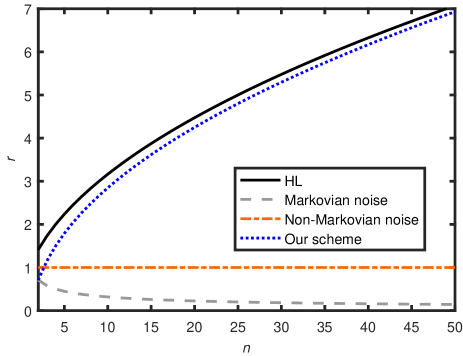
Figure 3: The relative ratio $r=\delta\phi|_{u}/\delta\phi|_{e}$ of the frequency resolutions of the entangled and unentangled probes when suffering from supercoherence. The black solid line represents the noise-free HL. When there are no auxiliary qubits, the gray dashed line shows the case of Markovian noise, and the red dash-dotted line shows the case of non-Markovian dynamics. And the blue dotted line shows our scheme with only one auxiliary qubit.

II.2.2 Uncorrelated Environment

When all probes are placed in an uncorrelated environment, e.g. spatially separated, the correlation function becomes $C_{ij}(0)=\gamma(t)\delta_{ij}$. And the quantum master Eq. (12) is simplified as

$$\dot{\rho} = i[\rho,H_{\textrm{S}}+H_{\textrm{LS}}]+\frac{1}{2}[\sum_{i}\gamma(t)(\sigma_{z}^{(i)}\rho\sigma_{z}^{(i)}-\rho)$$ (21)

$$+C_{aa}(0,t)(\sigma_{z}^{a}\rho\sigma_{z}^{a}-\rho)].$$

Let $K=g_{k}^{a}/g_{k}$. Consequently, we have $C_{aa}(0,t)=K^{2}\gamma(t)$. The off-diagonal element of the density matrix follows the evolution

$$\rho_{12}(t)=\rho_{12}(0)e^{i(N\Omega_{0}-\omega_{a})t}e^{-(N+K^{2})\int\gamma(t^{\prime})dt^{\prime}}.$$ (22)

Since $N+K^{2}>N$, using auxiliary qubits can not reduce but increase the dephasing of probes. As a consequence, our measurement scheme can not improve the precision of measurement in the case of uncorrelated environment.

II.2.3 Partially-Correlated Environment

In this subsection, we consider a partially-correlated environment. Assume that all qubits, including $N$ working qubits and one auxiliary qubit, are spatially arranged in a linear array, as shown in Fig. 1. Following Ref. (Jeske and Cole, 2013), the real-valued homogeneous correlation functions $C_{ij}(0,t)$, $C_{ia}(0,t)$ and $C_{ai}(0,t)$ read respectively

$$C_{ij}(0,t) = e^{-x|i-j|}\gamma(t),$$ (23)

$$C_{ia}(0,t) = C_{ai}(0,t)=Ke^{-x(N+1-i)}\gamma(t),$$ (24)

where $x=d/\xi$ with $d$ being the spatial distance between two adjacent qubits, $\xi$ is the environmental correlation length (Jeske and Cole, 2013). For an uncorrelated bath, we have $\xi=0$ and $C_{ij}=\delta_{ij}\gamma(t)$, while $\xi=\infty$ and $C_{ij}=\gamma(t)$ for any $i$ and $j$ in a fully-correlated bath. Generally, a finite but non-vanishing $\xi$ corresponds to a partially-correlated bath. The off-diagonal term of the density matrix is given by

$$\rho_{12}(t)=\rho_{12}(0)e^{i(N\Omega_{0}-\omega_{a})t}e^{-A(N,x)\int\gamma(t^{\prime})dt^{\prime}}.$$ (25)

where the factor

$$A(N,x) = (K-a)^{2}+b-a^{2},$$ (26)

$$a = \sum_{i=1}^{n}\exp[-x(N+1-i)],$$ (27)

$$b = \sum_{i,j=1}^{n}\exp(-x|i-j|).$$ (28)

Here, $A(N,a)\gamma(t)$ represents the total dephasing rate of the working and auxiliary qubits. In order to improve the precision of measurement, we can always choose a proper $K$ to minimize the factor $A(N,x)$. Therefore, employing auxiliary qubits can also improve the precision of a measurement for the entangled probes in a partially-correlated environment.

II.3 Example for Magnetic-Field Sensing

As known to all, the direction and magnitude of the geomagnetic field are closely related to the position on the earth. Thus, various schemes have been put forward to measure the magnetic field in order to utilize geomagnetic for navigation, e.g., radical pair mechanism Lambert et al. (2013) for avian navigation and the decoherence behaviors of the NV center in diamond Zhao et al. (2012); Li et al. (2017b); Jarmola et al. (2012); Yang et al. (2020); Head-Marsden et al. (2021). In this section, as an example, we show how to utilize our measurement scheme with one auxiliary qubit in magnetic-field sensing. The initial state of the entangled probes with $N$ working qubits and one auxiliary qubit is prepared in $|\Psi(0)\rangle=(|1\rangle_{a}|0\rangle^{\otimes N}+|0\rangle_{a}|1\rangle^{\otimes N})/\sqrt{2}$, where $|0\rangle$ and $|1\rangle$ refer to the parallel and antiparallel spin states with respect to the magnetic field, respectively. Then, let the probe be exposed to a magnetic field $B$. After a time interval $t$, it evolves into

$$\rho(t)\!\! = \!\!\frac{1}{2}[|1\rangle_{a}\langle 1|_{a}(|0\rangle\langle 0|)^{\otimes N}+|0\rangle_{a}\langle 0|_{a}(|1\rangle\langle 1|)^{\otimes N}$$ (29)

$$\!\!+e^{i(N\gamma_{0}B-\gamma_{a}B)t}e^{-\Gamma(t)}|1\rangle_{a}\langle 0|_{a}(|0\rangle\langle 1|)^{\otimes N}$$

$$\!\!+e^{-i(N\gamma_{0}B-\gamma_{a}B)t}e^{-\Gamma(t)}|0\rangle_{a}\langle 1|_{a}(|1\rangle\langle 0|)^{\otimes N}],$$

where $\gamma_{0}$ ($\gamma_{a}$) is the gyromagnetic ratio of the working (auxiliary) qubit. By choosing an appropriate auxiliary qubit which satisfies $g_{k}^{a}=Ng_{k}$, we have $\Gamma(t)=0$. The reduced density matrix of the working qubits at time $t$ is given by

$$\rho(t) = \frac{1}{2}[|1\rangle_{a}\langle 1|_{a}(|0\rangle\langle 0|)^{\otimes N}+|0\rangle_{a}\langle 0|_{a}(|1\rangle\langle 1|)^{\otimes N}$$ (30)

$$+e^{i(N\gamma_{0}B-\gamma_{a}B)t}|1\rangle_{a}\langle 0|_{a}(|0\rangle\langle 1|)^{\otimes N}$$

$$+e^{-i(N\gamma_{0}B-\gamma_{a}B)t}|0\rangle_{a}\langle 1|_{a}(|1\rangle\langle 0|)^{\otimes N}].$$

After a $pi/2$ pulse, the probability of finding the probes in their initial state reads $P=[1+\cos(N\gamma_{0}Bt-\gamma_{a}Bt)]/2$. Here, the Fisher information is given by

$$F(B)=\frac{(N\gamma_{0}-\gamma_{a})^{2}t^{2}\sin^{2}(N\gamma_{0}Bt-\gamma_{a}Bt)}{1-\cos^{2}(N\gamma_{0}Bt-\gamma_{a}Bt)}.$$ (31)

Since the best interrogation time for the entangled probes is determined by $(N\gamma_{0}B-\gamma_{a}B)t_{e}=k\pi/2$ with odd $k$, we calculate the uncertainty in the estimated value of $B$ as

$$\delta B^{2}|_{e}=\frac{1}{\left(N\gamma_{0}-\gamma_{a}\right)^{2}Tt}.$$ (32)

When $N$ is large enough, the precision of measurement will approach the HL.

III Quantum Simulation of Quantum Metrology

In the NMR platform, we can use bath-engineering technique and GRAPE algorithm to simulate the quantum dynamics under superdecoherence. By this quantum simulation, we can further prove that our measurement scheme with one auxiliary qubit can approach the HL, even in the case of superdecoherence. Utilizing the bath-engineering technique, we apply a time-dependent magnetic field to the total system including the working and auxiliary qubits. The total system is governed by the Hamiltonian (Wang et al., 2018; Zhang et al., 2021)

$$H=\frac{1}{2}\Omega_{0}\sum_{i=1}^{N}\sigma_{z}^{(i)}+\frac{1}{2}\omega_{a}\sigma_{z}^{a}+\beta_{1}(t)\sum_{i=1}^{N}\sigma_{z}^{(i)}+\beta_{2}(t)\sigma_{z}^{a},$$ (33)

with

$$\beta_{1}(t) = b_{1}\sum_{j=1}^{J}\omega_{j}F(j)\cos(\omega_{j}t+\psi_{1j}),$$ (34)

$$\beta_{2}(t) = b_{2}\sum_{j=1}^{J}\omega_{j}F(j)\cos(\omega_{j}t+\psi_{2j}),$$ (35)

where $b_{1}$ and $b_{2}$ are the noise amplitudes perceived by the working and auxiliary qubits, respectively. $\omega_{0}$ ($\omega_{J}=J\omega_{0}$) is the base (cutoff) frequency with $\omega_{j}=j\omega_{0}$. $F(j)$ is the function which determines the type of noise, and $\psi_{ij}$ ($i=1,2$) is a random number. All the parameters above can be manipulated manually. Here, we apply identical time-dependent magnetic fields to all of the working qubits to simulate the superdecoherence. We further assume $b_{2}=nb_{1}$ and $\psi_{1j}=\psi_{2j}$ to cancel the effects of the noise by the auxiliary qubit.

We divide the Hamiltonian (33) into two parts, i.e., the control Hamiltonian $H_{c}=(\Omega_{0}\sum_{i=1}^{N}\sigma_{z}^{(i)}+\omega_{a}\sigma_{z}^{a})/2$, and the noise Hamiltonian $H_{0}(t)=\beta_{1}(t)\sum_{i=1}^{N}\sigma_{z}^{(i)}+\beta_{2}(t)\sigma_{z}^{a}$. In the Schrödinger picture, the propagator of this dynamics is given by

$$U(t) = U_{c}(t)\tilde{U}(t)$$ (36)

where

$$U_{c}(t) = e^{-\frac{i}{2}(\Omega_{0}t\sum_{i}\sigma_{z}^{(i)}+\omega_{a}t\sigma_{z}^{a})},$$

$$\tilde{U}(t) = e^{-i\int_{0}^{t}d\tau\beta_{1}(\tau)\sum_{i}\sigma_{z}^{(i)}}e^{-i\int_{0}^{t}d\tau\beta_{2}(\tau)\sigma_{z}^{a}}.$$ (37)

The initial state of the total system is $|\Psi(0)\rangle=[|1\rangle_{a}|0\rangle^{\otimes N}+|0\rangle_{a}|1\rangle^{\otimes N}]/\sqrt{2}$. Let it evolve for a time interval $t$ under the Hamiltonian (33). Thus, we have

$$|\psi(t)\rangle\!\! = \!\!U(t)|\psi(0)\rangle$$ (38)

$$= \!\!\frac{1}{\sqrt{2}}(e^{-i\phi(t)}|1\rangle_{a}|0\rangle^{\otimes N}+e^{i\phi(t)}|0\rangle_{a}|1\rangle^{\otimes N}),$$

with

$$\phi(t) = \phi_{A}(t)+\phi_{B}(t),$$

$$\phi_{A}(t) = \frac{1}{2}(N\Omega_{0}-\omega_{a})t,$$

$$\phi_{B}(t) = \frac{1}{2}[N\int_{0}^{t}d\tau\beta_{1}(\tau)-\int_{0}^{t}d\tau\beta_{2}(\tau)].$$ (39)

In order to mimic the effect of decoherence, we prepare a large number of ensemble which evolve under different Hamiltonians characterized by a set of the random numbers $\{\psi_{1j},\psi_{2j}\}$. Finally, the probability of finding the probes in the initial state is over the ensemble as

$$P_{0}(t)\!\!=\!\!\frac{1}{2}[1+\cos 2\phi_{A}\langle\cos 2\phi_{B}\rangle-\sin 2\phi_{A}\langle\sin 2\phi_{B}\rangle].$$ (40)

If we further assume a Gaussian noise, then we have $\langle\phi_{B}^{2m-1}(t)\rangle=0$ for any positive integer $m$ (Wang et al., 2018), and thus yields

$$P_{0}(t)=\frac{1}{2}[1+\cos 2\phi_{A}(t)e^{-2\chi(t)}],$$ (41)

where

$$\chi(t)\!\! = \!\!\langle\phi_{B}^{2}(t)\rangle=\frac{4}{2\pi}\smallint_{-\infty}^{+\infty}\frac{d\omega}{\omega^{2}}S(\omega)\sin^{2}\frac{\omega t}{2},$$

$$S(\omega)\!\! = \!\!\frac{1}{4}[N^{2}S_{11}(\omega)-NS_{12}(\omega)-NS_{21}(\omega)+S_{22}(\omega)].$$

Here, $S_{ij}(\omega)=\smallint_{-\infty}^{+\infty}dt\langle\beta_{i}(0)\beta_{j}(t)\rangle\exp(i\omega t)$ $(i,j=1,2)$ is the Fourier transform of the two-time correlation function $\langle\beta_{i}(t_{1})\beta_{j}(t_{2})\rangle$, which depends on the time interval $t_{2}-t_{1}$. And $S(\omega)$ is the total power spectral density of the noise, which describes the energy distribution of the stochastic signal in the frequency domain (Wang et al., 2018).

We utilize the relation that $b_{2}=Nb_{1}$ and $\psi_{1j}=\psi_{2j}$ to obtain the two-time correlation functions as

$$\langle\beta_{1}(t+\tau)\beta_{1}(t)\rangle\!\! = \!\!\frac{b_{1}^{2}\omega_{0}^{2}}{2}\sum_{j=1}^{J}j^{2}F(j)^{2}\cos(\omega_{j}\tau),$$

$$\langle\beta_{1}(t+\tau)\beta_{2}(t)\rangle\!\! = \!\!\langle\beta_{2}(t+\tau)\beta_{1}(t)\rangle$$

$$= \!\!\frac{Nb_{1}^{2}\omega_{0}^{2}}{4}\sum_{j=1}^{J}j^{2}F(j)^{2}\cos(\omega_{j}\tau),$$

$$\langle\beta_{2}(t+\tau)\beta_{2}(t)\rangle\!\! = \!\!\frac{N^{2}b_{1}^{2}\omega_{0}^{2}}{2}\sum_{j=1}^{J}j^{2}F(j)^{2}\cos(\omega_{j}\tau).$$

Thus, the power spectral densities are respectively given by

$$S_{11}(\omega) = \frac{\pi b_{1}^{2}\omega_{0}^{2}}{2}\sum_{j=1}^{J}j^{2}F(j)^{2}[\delta(\omega-\omega_{j})+\delta(\omega+\omega_{j})],$$

$$S_{12}(\omega) = S_{21}(\omega)$$

$$= \frac{N\pi b_{1}^{2}\omega_{0}^{2}}{2}\sum_{j=1}^{J}j^{2}F(j)^{2}[\delta(\omega-\omega_{j})+\delta(\omega+\omega_{j})],$$

$$S_{22}(\omega)\!\! = \!\!\frac{N^{2}\pi b_{1}^{2}\omega_{0}^{2}}{2}\sum_{j=1}^{J}j^{2}F(j)^{2}[\delta(\omega-\omega_{j})\!+\!\delta(\omega+\omega_{j})].$$

Obviously, the total power spectral density reads

$$S\left(\omega\right)=N^{2}S_{11}\left(\omega\right)-NS_{12}\left(\omega\right)-NS_{21}\left(\omega\right)+S_{22}\left(\omega\right)=0,$$

and the decoherence function also vanishes, i.e.,

$$\chi(t)=\frac{4}{2\pi}\smallint_{-\infty}^{+\infty}\frac{d\omega}{\omega^{2}}S\left(\omega\right)\sin^{2}\frac{\omega t}{2}=0.$$

We calculate the uncertainty of the measurement by the Fisher information as

$$\delta\Omega_{0}^{2}=\frac{1}{\left(T/t\right)F\left(\phi\right)}=\frac{1-\cos^{2}\left[\left(N\omega_{0}-\omega_{a}\right)t\right]}{N^{2}Tt\sin^{2}\left[\left(N\omega_{0}-\omega_{a}\right)t\right]}.$$ (42)

By similar derivation to Eq. (19), we have $\delta\Omega_{0}^{2}\mid_{e}\propto\left(n-1\right)^{-2}$. We find the scaling law for our scheme can approach the HL when $N$ is large enough, even in the case of superdecoherence.

We apply the quantum simulation algorithm to simulate our scheme as shown in Fig. 4. We use the same types of lines as Fig. 2 to represent the probability. Here, the number of random realizations in ensemble we used in this simulation is $2\times 10^{3}$. The time steps between the dots are 5 ms. Without loss of generality, we assume the model of white noise, i.e., $F(j)=1/j$ Soare et al. (2014b). The base and cutoff frequencies for the Markovian noise are $\omega_{0}=0.2$ Hz and $\omega_{c}=140$ Hz, respectively, while for the non-Markovian noise, we use the following parameters $\omega_{0}=10^{-3}$ Hz and $\omega_{c}=0.18$ Hz. We can learn from Fig. 4 that the results of stochastic Hamiltonian simulation are in quite-good agreement with the results of the Bloch-Redfield equation. The blue square dots represent our scheme, which implies that employing one auxiliary qubit can cancel the effects of noise. As a result, the precision in our scheme can approach the HL. In order to explore the underlying physical mechanism explicitly, we also plot the corresponding decoherence factor $\Gamma(t)$ in Fig. 5. For the Markovian noise, the coherence decays with a constant rate, and thus using entangled probes will not improve the precision of the estimation. For the non-Markovian noise, since the coherence decays quadratically with time, the use of entangled probe can offer a better estimation, but the precision is still lower than the HL. However, for a correlated bath, because all qubits suffer from the collective noise, by properly arranging the auxiliary qubit the noises on the working qubits can be effectively canceled and thus the noise-free measurement can be performed.

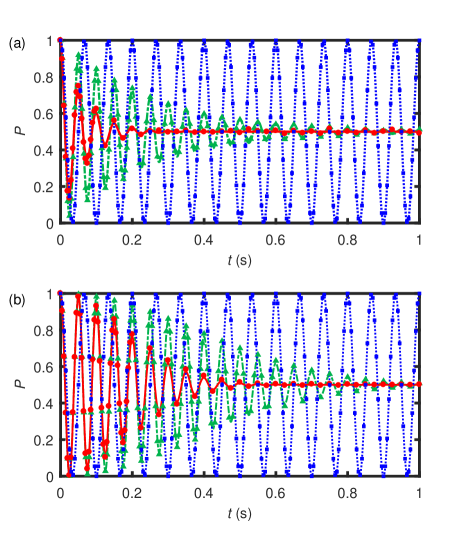
Figure 4: Quantum simulation of population dynamics in Fig. 2. The dashed green line, the solid red line and the dotted blue line are the same as Fig. 2, while the green triangles, the red circle and the blue squares are obtained by the quantum simulation approach Wang et al. (2018); Zhang et al. (2021) for the uncorrelated decoherence, the superdecoherence and our scheme, respectively.

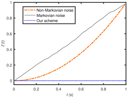
Figure 5: The simulated decoherence factor $\Gamma(t)$ for different schemes: the gray solid line for Markovian environment, the red dash-dotted line for non-Markovian environment, and the blue dotted line for our scheme.

IV Conclusion

In this paper, we propose a quantum metrology scheme with auxiliary states. The auxiliary states are properly designed and can selectively offset the impact of environmental noise. On account of superdecoherence, we analyze the optimal precision with and without auxiliary qubits. We find out that when the auxiliary qubits are not employed, the precision can not be improved by using the entangled probes no matter whether the noise is Markovian or non-Markovian. However, utilizing an auxiliary qubit can make the precision approach the HL in our scheme. We further discuss the cases of uncorrelated and partially-correlated environment, and find out that employing auxiliary qubits can improve the precision of measurement in the partially-correlated environment but it fails in the uncorrelated environment. As an example, we show how to utilize our scheme with one auxiliary qubit in magnetic-field sensing. Finally, we use the bath-engineering technique and GRAPE to simulate the quantum dynamics and demonstrate that assisted by an auxiliary qubit our scheme can approach the HL in the case of superdecoherence.

We thank valuable discussions with M.-J. Tao. This work is supported by the National Natural Science Foundation of China under Grant Nos. 11674033, 11474026, 11505007, and Beijing Natural Science Foundation under Grant No. 1202017.

*

Appendix A Dynamics of n-qubit Decoherence

The quantum dynamics of open system is described by the well-known spin-boson model (Leggett et al., 1987). Since the time scale of dephasing is generally much smaller than that of longitudinal relaxation, we consider the pure-dephasing dynamics for simplicity. The spin-boson Hamiltonian of $n$ qubits coupled to a common bath can be written as (Breuer et al., 2016; Jeske and Cole, 2013; Piilo et al., 2008; Ai et al., 2014)

$$H=\frac{1}{2}\omega_{0}\sum_{i=1}^{n}\sigma_{z}^{(i)}+\sum_{k}\omega_{k}b_{k}^{\dagger}b_{k}+\sum_{i=1}^{n}\sigma_{z}^{(i)}\sum_{k}g_{k}^{(i)}(b_{k}^{\dagger}+b_{k}).$$ (43)

Assuming that $\hbar=1$, the system Hamiltonian is $H_{\textrm{S}}=\omega_{0}\sum_{i=1}^{n}\sigma_{z}^{(i)}/2$, and the bath Hamiltonian is $H_{\textrm{B}}=\sum_{k}\omega_{k}b_{k}^{\dagger}b_{k}$, and the interaction Hamiltonian is $H_{\textrm{I}}=\sum_{i=1}^{n}\sigma_{z}^{(i)}\sum_{k}g_{k}^{(i)}(b_{k}^{\dagger}+b_{k})$, where $\omega_{0}$ is the energy separation between the ground and excited states, $b_{k}^{\dagger}$ ($b_{k}$) is the creation (annihilation) bath operator, $g_{k}$ is the coupling constant between the qubit and $k$th mode of bath, which is assumed to be real for simplicity.

The interaction Hamiltonian is the product of the system operators and the bath operators, i.e., $H_{\textrm{I}}=\sum_{i=1}^{n}s_{i}B_{i}$ with $s_{i}=\sigma_{z}^{(i)}$ and $B_{i}=\sum_{k}g_{k}^{(i)}(b_{k}^{\dagger}+b_{k})$. We decompose the system operators $s_{i}$ into several parts in the eigenspace $\{|\epsilon\rangle_{i}\}$ as $s_{i}=\sum_{\omega}s_{i}(\omega)|\epsilon\rangle_{i}\langle\epsilon^{\prime}|$ with $s_{i}(\omega)=\sum_{\epsilon^{\prime}-\epsilon=\omega}\langle\epsilon|s_{i}|\epsilon^{\prime}\rangle_{i}$. The summation in $s_{i}(\omega)$ is extended over all energy eigenvalues $\epsilon$ and $\epsilon^{\prime}$ of $H_{S}$ with a fixed energy difference of $\omega$ (Jeske and Cole, 2013; Breuer and Petruccione, 2002). Because $s_{i}=\sigma_{z}^{(i)}$, we have $s_{i}(\omega_{0})=s_{i}(-\omega_{0})=0$ and $s_{i}(0)=\mp 1$ for $|0\rangle_{i}$ and $|1\rangle_{i}$, respectively. Introducing these eigenoperator decompositions, the Bloch-Redfield equations can be rewritten as

$$\dot{\rho}=i[\rho,H_{\textrm{S}}]+\sum_{i,j=1}^{n}D_{ij}(0,t)(\sigma_{z}^{(j)}\rho\sigma_{z}^{(i)}-\frac{1}{2}\{\sigma_{z}^{(i)}\sigma_{z}^{(j)},\rho\}),$$ (44)

where $D_{ij}(\omega,t)=\intop_{0}^{t}d\tau\exp(i\omega\tau)\langle\widetilde{B}_{i}(\tau)\widetilde{B}_{j}(0)\rangle$ are the spectral functions, which define both temporal and spatial correlations of the pure-dephasing noise environment (Jeske et al., 2015). $\widetilde{B}_{i}(\tau)=g_{k}^{(i)}[b_{k}^{\dagger}\exp(i\omega_{k}\tau)+b_{k}\exp(-i\omega_{k}\tau)]$ are the operators of environment in the interaction picture, and $\langle\widetilde{B}_{i}(\tau)\widetilde{B}_{j}(0)\rangle$ are the correlation functions, i.e.,

$$\langle\widetilde{B}_{i}(\tau)\widetilde{B}_{j}(0)\rangle=\sum_{k}g_{k}^{(i)}g_{k}^{(j)}[2\overline{n}(\omega_{k},T)\cos\omega_{k}\tau+e^{-i\omega_{k}\tau}].$$

Thus, the spectral functions are explicitly given as

$$D_{ij}(\omega,t) = \sum_{k}g_{k}^{(i)}g_{k}^{(j)}[2\overline{n}(\omega_{k},T)\frac{\sin\omega_{k}t}{\omega_{k}}$$ (46)

$$+\frac{1-e^{-i\omega_{k}t}}{i\omega_{k}}]|_{\omega_{k}=\omega},$$

where $\overline{n}(\omega_{k},T)=\langle b_{k}^{\dagger}b_{k}\rangle$ denotes the average occupation number of mode $k$ at temperature $T$. The real part of $D_{ij}(0,t)$ causes dephasing while its imaginary part corresponds to Lamb shift (Jeske and Cole, 2013). Let $D_{ij}(0,t)=\frac{1}{2}C_{ij}(0,t)+iF_{ij}(0,t)$, and $H_{\textrm{LS}}=\sum_{i,j=1}^{n}F_{ij}(0,t)\sigma_{z}^{(i)}\sigma_{z}^{(j)}$ is the Lamb-shift Hamiltonian. Thus, Eq. (44) is rewritten as

$$\dot{\rho} = i[\rho,H_{\textrm{S}}+H_{\textrm{LS}}]$$

$$+\frac{1}{2}\sum_{i,j=1}^{n}C_{ij}(0,t)(\sigma_{z}^{(j)}\rho\sigma_{z}^{(i)}-\frac{1}{2}\{\sigma_{z}^{(i)}\sigma_{z}^{(j)},\rho\}).$$

For $n=1$, since the total Hamiltonian is $H=\omega_{0}\sigma_{z}/2+\sum_{k}\omega_{k}b_{k}^{\dagger}b_{k}+\sigma_{z}\sum_{k}g_{k}(b_{k}^{\dagger}+b_{k})$, Eq. (A) is simplified as

$$\dot{\rho}=i[\rho,\frac{1}{2}\omega_{0}\sigma_{z}]+C(0,t)(\sigma_{z}\rho\sigma_{z}-\rho),$$ (48)

where the single-qubit dephasing rate is given by $\gamma(t)=C(0,t)$.

However, the $n$-qubit dephasing rate varies with the environmental model. For simplicity, we assume that $g_{k}^{(i)}=g_{k}^{(j)}=g_{k}$. When $n$ qubits are in an uncorrelated environment, e.g. the distance between the qubits are far beyond the correlation length of the environment (Jeske and Cole, 2013), we can neglect all spatial correlations of the bath, i.e., $C_{ij}(0,t)=\gamma(t)\delta_{ij}$. Hence $\gamma_{n}(t)=\sum_{i,j=1}^{n}C_{i,j}(0,t)=n\gamma(t)$. In contrast, when $n$ qubits are in a correlated bath, i.e., the correlation length of the environment is much bigger than the qubits’ spatial separation, the $n$-qubit dephasing rate is $n^{2}$ times that of single qubit, i.e., $\gamma_{n}(t)=n^{2}\gamma(t)$, resulting from $C_{ij}(0,t)=\gamma(t)$ for all $i$ and $j$. This phenomenon is called superdecoherence, mainly due to collective entanglement between qubits and environment (Palma et al., 1996).

References

- Giovannetti et al. (2011) V. Giovannetti, S. Lloyd, and L. Maccone, Advances in quantum metrology, Nat. Photon. 5, 222 (2011).
- Degen et al. (2017) C. L. Degen, F. Reinhard, and P. Cappellaro, Quantum sensing, Rev. Mod. Phys. 89, 035002 (2017).
- Nielsen and Chuang (2000) M. A. Nielsen and I. L. Chuang, Quantum Computation and Quantum Information (Cambridge University Press, 2000).
- Lambert et al. (2013) N. Lambert, Y. N. Chen, Y. C. Cheng, C. M. Li, G. Y. Chen, and F. Nori, Quantum biology, Nat. Phys. 9, 10 (2013).
- Ai et al. (2013a) Q. Ai, T. C. Yen, B. Y. Jin, and Y. C. Cheng, Clustered geometries exploiting quantum coherence effects for efficient energy transfer in light harvesting, J. Phys. Chem. Lett. 4, 2577 (2013a).
- Cai et al. (2012) C. Y. Cai, Q. Ai, H. T. Quan, and C. P. Sun, Sensitive chemical compass assisted by quantum criticality, Phys. Rev. A 85, 022315 (2012).
- Yang et al. (2012) L. P. Yang, Q. Ai, and C. P. Sun, Generalized Holstein model for spin-dependent electron-transfer reactions, Phys. Rev. A 85, 032707 (2012).
- Cai and Plenio (2013) J. M. Cai and M. B. Plenio, Chemical compass model for avian magnetoreception as a quantum coherent device, Phys. Rev. Lett. 111, 230503 (2013).
- Oktel and Müstecaplıoğlu (2004) M. Ö. Oktel and Ö. E. Müstecaplıoğlu, Electromagnetically induced left-handedness in a dense gas of three-level atoms, Phys. Rev. A 70, 053806 (2004).
- Thommen and Mandel (2006) Q. Thommen and P. Mandel, Electromagnetically induced left handedness in optically excited four-Level atomic media, Phys. Rev. Lett. 96, 053601 (2006).
- Kästel et al. (2007) J. Kästel, M. Fleischhauer, S. F. Yelin, and R. L. Walsworth, Tunable negative refraction without absorption via electromagnetically induced chirality, Phys. Rev. Lett. 99, 073602 (2007).
- Zhao et al. (2020) J. X. Zhao, J. J. Cheng, Y. Q. Chu, Y. X. Wang, F. G. Deng, and Q. Ai, Hyperbolic metamaterial using chiral molecules, Sci. China-Phys. Mech. Astron. 63, 260311 (2020).
- Braunstein (1992) S. L. Braunstein, Quantum limits on precision measurements of phase, Phys. Rev. Lett. 69, 3598 (1992).
- Giovannetti et al. (2004) V. Giovannetti, S. Lloyd, and L. Maccone, Quantum-enhanced measurements: Beating the standard quantum limit, Science 306, 5700 (2004).
- Leibfried et al. (2004) D. Leibfried, M. D. Barrett, T. Schaetz, J. Britton, J. Chiaverini, W. M. Itano, J. D. Jost, C. Langer, and D. J. Wineland, Toward Heisenberg-limited spectroscopy with multiparticle entangled states, Science 304, 5676 (2004).
- Roos et al. (2006) C. Roos, M. Chwalla, K. Kim, M. Riebe, and R. Blatt, Designer atoms’ for quantum metrology, Nature(London) 443, 316 (2006).
- Breuer et al. (2016) H.-P. Breuer, E.-M. Laine, J. Piilo, and B. Vacchini, Colloquium: Non-Markovian dynamics in open quantum systems, Rev. Mod. Phys. 88, 021002 (2016).
- de Vega and Alonso (2017) I. de Vega and D. Alonso, Dynamics of non-Markovian open quantum systems, Rev. Mod. Phys. 89, 015001 (2017).
- Li et al. (2018) L. Li, M. J. W. Hall, and H. M. Wiseman, Concepts of quantum non-Markovianity: A hierarchy, Phys. Rep. 759, 1 (2018).
- Breuer et al. (2009) H.-P. Breuer, E.-M. Laine, and J. Piilo, Degree of non-Markovian behavior of quantum processes in open systems, Phys. Rev. Lett. 103, 210401 (2009).
- Liu et al. (2011) B.-H. Liu, L. Li, Y.-F. Huang, C.-F. Li, G.-C. Guo, E.-M. Laine, H.-P. Breuer, and J. Piilo, Experimental control of the transition from Markovian to non-Markovian dynamics of open quantum systems, Nat. Phys. 7, 931 (2011).
- Rivas et al. (2010) A. Rivas, S. F. Huelga, and M. B. Plenio, Entanglement and non-Markovianity of quantum evolutions, Phys. Rev. Lett. 105, 050403 (2010).
- Childress et al. (2006) L. Childress, M. V. G. Dutt, J. M. Taylor, A. S. Zibrov, F. Jelezko, J. Wrachtrup, P. R. Hemmer, and M. D. Lukin, Coherent dynamics of coupled electron and nuclear spin qubits in diamond, Science 314, 281 (2006).
- Chin et al. (2012) A. W. Chin, S. F. Huelga, and M. B. Plenio, Quantum metrology in non-Markovian environments, Phys. Rev. Lett. 109, 233601 (2012).
- Kattemölle and van Wezel (2020) J. Kattemölle and J. van Wezel, Conditions for superdecoherence, Quantum 4, 265 (2020).
- Dorner (2012) U. Dorner, Quantum frequency estimation with trapped ions and atoms, New J. Phys. 14, 043011 (2012).
- Yousefjani et al. (2017) R. Yousefjani, S. Salimi, and A. S. Khorashad, Enhancement of frequency estimation by spatially correlated environments, Ann. Phys. (N.Y.) 381, 80 (2017).
- Song et al. (2016) X.-K. Song, H. Zhang, Q. Ai, J. Qiu, and F.-G. Deng, Shortcuts to adiabatic holonomic quantum computation in decoherence-free subspace with transitionless quantum driving algorithm, New J. Phys. 18, 023001 (2016).
- Soare et al. (2014a) A. Soare, H. Ball, D. Hayes, J. Sastrawan, M. C. Jarratt, J. J. McLoughlin, X. Zhen, T. J. Green, and M. J. Biercuk, Experimental noise filtering by quantum control, Nat. Phys. 10, 825 (2014a).
- Soare et al. (2014b) A. Soare, H. Ball, D. Hayes, X. Zhen, M. C. Jarratt, J. Sastrawan, H. Uys, and M. J. Biercuk, Experimental bath engineering for quantitative studies of quantum control, Phys. Rev. A 89, 042329 (2014b).
- Khaneja et al. (2005) N. Khaneja, T. Reiss, C. Kehlet, and T. SchulteHerbrüggen, Optimal control of coupled spin dynamics: design of NMR pulse sequences by gradient ascent algorithms, J. Magn. Reson. 172, 296 (2005).
- Li et al. (2017a) J. Li, X. D. Yang, X. H. Peng, and C. P. Sun, Hybrid quantum-classical approach to quantum optimal control, Phy. Rev. Lett. 118, 150503 (2017a).
- Wang et al. (2018) B.-X. Wang, M.-J. Tao, Q. Ai, T. Xin, N. Lambert, D. Ruan, Y.-C. Cheng, F. Nori, F.-G. Deng, and G.-L. Long, Efficient quantum simulation of photosynthetic light harvesting, npj Quantum Inf. 4, 52 (2018).
- Zhang et al. (2021) N.-N. Zhang, M.-J. Tao, W.-T. He, X.-Y. Chen, X.-Y. Kong, F.-G. Deng, N. Lambert, and Q. Ai, Efficient quantum simulation of open quantum dynamics at various Hamiltonians and spectral densities, Front. Phys. 16, 51501 (2021).
- Buluta and Nori (2009) I. Buluta and F. Nori, Quantum simulators, Science 326, 108 (2009).
- Georgescu et al. (2014) I. M. Georgescu, S. Ashhab, and F. Nori, Quantum simulation, Rev. Mod. Phys. 86, 153 (2014).
- Huelga et al. (1997) S. F. Huelga, C. Macchiavello, T. Pellizzari, and A. K. Ekert, Improvement of frequency standards with quantum entanglement, Phys. Rev. Lett. 79, 3865 (1997).
- Breuer and Petruccione (2002) H. P. Breuer and F. Petruccione, The Theory of Open Quantum Systems (Oxford University Presss, 2002).
- Liu et al. (2017) P. Liu, P. Wang, W. Yang, G. R. Jin, and C. P. Sun, Fisher information of a squeezed-state interferometer with a finite photon-number resolution, Phys. Rev. A 95, 023824 (2017).
- Ai et al. (2010) Q. Ai, Y. Li, H. Zheng, and C. P. Sun, Quantum anti-Zeno effect without rotating wave approximation, Phys. Rev. A 81, 042116 (2010).
- Ai et al. (2013b) Q. Ai, D. Xu, S. Yi, A. G. Kofman, C. P. Sun, and F. Nori, Quantum anti-Zeno effect without wave function reduction, Sci. Rep. 3, 1752 (2013b).
- Harrington et al. (2017) P. M. Harrington, J. T. Monroe, and K. W. Murch, Quantum Zeno effects from measurement controlled qubit-bath interactions, Phys. Rev. Lett. 118, 240401 (2017).
- Jeske and Cole (2013) J. Jeske and J. H. Cole, Derivation of Markovian master equations for spatially correlated decoherence, Phys. Rev. A 87, 052138 (2013).
- Zhao et al. (2012) N. Zhao, S.-W. Ho, and R.-B. Liu, Decoherence and dynamical decoupling control of nitrogen vacancy center electron spins in nuclear spin baths, Phys. Rev. B 85, 115303 (2012).
- Li et al. (2017b) L.-S. Li, H.-H. Li, L.-L. Zhou, Z.-S. Yang, and Q. Ai, Measurement of weak static magnetic field with nitrogen-vacancy color center, Acta Phys. Sin. 66, 230601 (2017b).
- Jarmola et al. (2012) A. Jarmola, V. M. Acosta, K. Jensen, S. Chemerisov, and D. Budker, Temperature- and Magnetic-Field-Dependent Longitudinal Spin Relaxation in Nitrogen-Vacancy Ensembles in Diamond, Phys. Rev. Lett. 108, 197601 (2012).
- Yang et al. (2020) Z.-S. Yang, Y.-X. Wang, M.-J. Tao, W. Yang, M. Zhang, Q. Ai, and F.-G. Deng, Longitudinal relaxation of a nitrogen-vacancy center in a spin bath by generalized cluster-correlation expansion method, Annals of Physics 413, 168063 (2020).
- Head-Marsden et al. (2021) K. Head-Marsden, J. Flick, C. J. Ciccarino, and P. Narang, Quantum Information and Algorithms for Correlated Quantum Matter, Chemical Reviews 121, 3061 (2021).
- Leggett et al. (1987) A. J. Leggett, S. Chakravarty, A. T. Dorsey, M. P. A. Fisher, A. Garg, and W. Zwerger, Dynamics of the dissipative two-state system, Rev. Mod. Phys. 59, 1 (1987).
- Piilo et al. (2008) J. Piilo, S. Maniscalco, K. Härköenen, and K.-A. Suominen, Non-Markovian quantum jumps, Phys. Rev. Lett. 100, 180402 (2008).
- Ai et al. (2014) Q. Ai, Y. J. Fan, B. Y. Jin, and Y. C. Cheng, An efficient quantum jump method for coherent energy transfer dynamics in photosynthetic systems under the influence of laser fields, New J. Phys 16, 053033 (2014).
- Jeske et al. (2015) J. Jeske, D. J. Ing, M. B. Plenio, S. F. Huelga, and J. H. Cole, Bloch-Redfield equations for modeling light-harvesting complexes, J. Chem. Phys. 142, 064104 (2015).
- Palma et al. (1996) G. M. Palma, K.-A. Suominen, and A. Ekert, Quantum computers and dissipation, Proc. R. Soc. Lond. A. 452, 567 (1996).