]gplatero@icmm.csic.es
Tunable zero modes and quantum interferences in flat-band topological insulators
Abstract
We investigate the interplay between Aharonov-Bohm (AB) caging and topological protection in a family of quasi-one-dimensional topological insulators, which we term CSSH ladders. Hybrids of the Creutz ladder and the SSH chain, they present a regime with completely flat bands, and a rich topological phase diagram, with several kinds of protected zero modes. These are reminiscent of the Creutz ladder edge states in some cases, and of the SSH chain edge states in others. Furthermore, their high degree of tunability, and the fact that they remain topologically protected even in small systems in the rungless case, due to AB caging, make them suitable for quantum information purposes. One of the ladders can belong to the BDI, AIII and D symmetry classes depending on its parameters, the latter being unusual in a non-superconducting model. Two of the models can also harbor topological end modes which do not follow the usual bulk-boundary correspondence, and are instead related to a Chern number. Finally, we propose some experimental setups to implement the CSSH ladders with current technology, focusing on the photonic lattice case.
1 Introduction
Topological materials have a gapped bulk, which can be insulating or superconducting, and a metallic surface spectrum. For one-dimensional (1D) materials, this implies the existence of topological zero modes, robust end states pinned at zero energy and protected by symmetries of the Hamiltonian. Depending on these symmetries, topological materials can be classified into ten topological phases, five of which can show topological phases in 1D [1].
The robustness of their topological end modes can serve as a way to prevent errors in quantum information protocols. For instance, the well-known SSH chain end modes can be used as a way to implement a robust quantum state transfer protocol [2, 3, 4, 5, 6], or a quantum memory resistant to off-diagonal disorder [5]. Ladder models are quasi-1D lattice models that consist of two chains of sites coupled by tunneling amplitudes or interactions. By tuning the different parameters in ladder models, several BDI [7, 8, 9, 10], AIII [11, 12, 10, 13, 14] and CII [15, 16] topological insulators (TIs) have been found. The best-known topological ladder model is probably the Creutz ladder [17], a BDI topological insulator that also shows flat bands in a certain regime, where particles experience a self-localization phenomenon termed “Aharonov-Bohm (AB) caging” due to a magnetic flux. This effect has previously been studied in other 1D and 2D lattices, like the rhombus chain [18, 19, 20, 21] and the and lattices [22, 23], and has been observed experimentally in several setups [24, 25, 26, 27, 28, 29].
Flat-band models have attracted a great deal of research in recent years, in part because of the discovery of magic-angle twisted bilayer graphene [30]. The Creutz ladder and other quasi-1D flat-band models like the rhombus chain can serve as toy models to explore the interplay of localization dynamics with interactions or topology [20, 7, 31, 32, 33, 21]. Other studied variants of the Creutz ladder include additional Peierls phases or on-site energies [34, 12, 13, 11], Floquet driving [35, 36], spin- particles [37, 35, 16] or superconductivity [38, 32].
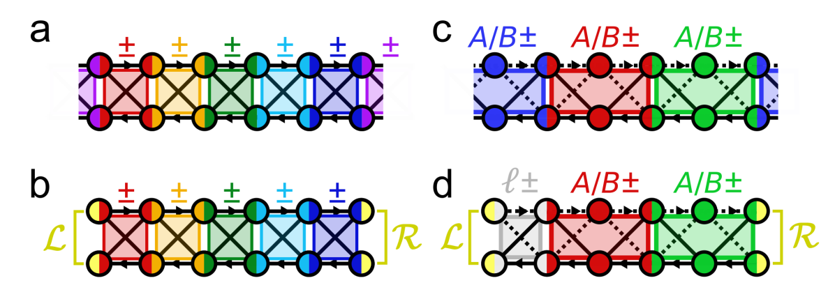
In this work, we propose and investigate a family of quasi-1D topological insulators related to the Creutz ladder and the SSH chain, which we term Creutz-Su-Schrieffer-Heeger (CSSH) ladders [see Figs. 1 and 2]. They present a regime where all four bands are flat due to AB caging. This phenomenon also localizes the edge states in one or two sites whenever the vertical links of the ladders vanish. This prevents the overlap of the left and right states, and allows them to be degenerate at zero energy even in small systems. This unusual interplay between quantum interference and topology, inherited from the Creutz ladder, enhances the topological protection of the states, which is preserved even in the one-plaquette limit of the ladders. A remarkable result of our work is that, in the CSSH ladders, the wavefunction of these end states can be tuned, using the parameters of the model, to take the form of almost any state in the Bloch sphere spanned by the two end sites. This can be used to prepare the Creutz ladder end states starting from a particle in a single site, or to control a particle in a topologically protected way even in small systems, something that can be useful for quantum information purposes.
Interestingly, one of the models, the hourglass CSSH ladder, can harbor topological zero modes reminiscent of both the Creutz ladder and the SSH chain end states. Another one of them, the delta CSSH ladder, has topological phases in the BDI, AIII and D classes, such that these three classes can be explored by changing the parameters of the system, without closing the gap or losing the protection of the states. This is something remarkable, because models in the D class in 1D are usually topological superconductors [39, 40]. In the rhomboid and delta CSSH ladders, we also report the existence non-protected topological end modes which do not follow the usual bulk-boundary correspondence. They can instead be related to a Chern number, even though they appear in a quasi-1D model. These modes are very similar to those found in the trimer chain [41]. The mentioned features make the CSSH ladders versatile and exotic models, which can also be realized experimentally in several bosonic and fermionic platforms with current technology.
In Section 2, we present the Hamiltonian of the CSSH ladders. Then, in section 3, we review the topology of the SSH chain and the Creutz ladder, including an original full description of the symmetries of the latter. In Section 4, we discuss the topological phase diagrams of the models, their spectra, symmetries and zero modes. In Section 5 we propose some experimental implementations of the models, focusing on the photonic lattice case. Finally, in Section 6, we present our conclusions.
2 The CSSH ladder models
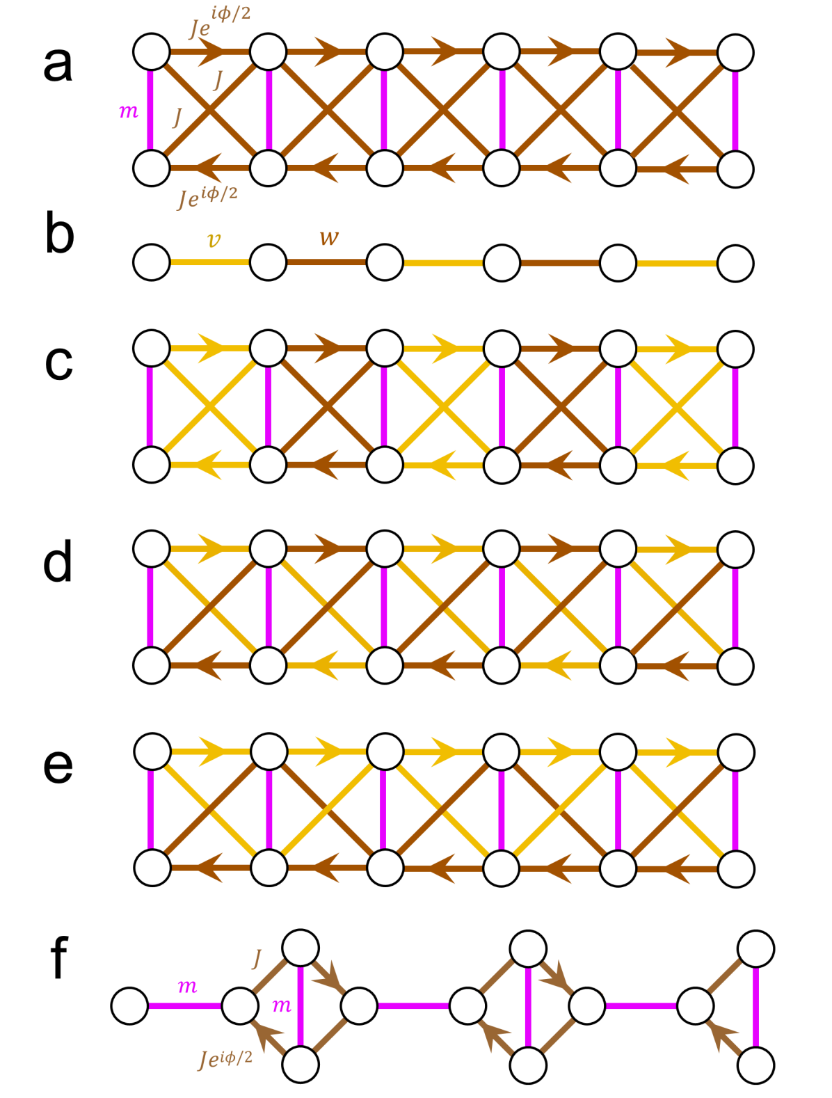
The Creutz ladder [17, 11, 33], a quasi-1D topological insulator, is formed by two chains of sites, connected by vertical, horizontal, and diagonal links [see Fig. 2 (a)]. A magnetic field is applied in the perpendicular direction. On the other hand, the Su-Schrieffer-Heeger (SSH) chain [42, 43], the simplest 1D TI, consists of a chain of sites connected by alternate hopping amplitudes [see Fig. 2 (b)]. Both systems are chiral TIs for some values of their parameters (see Section 3).
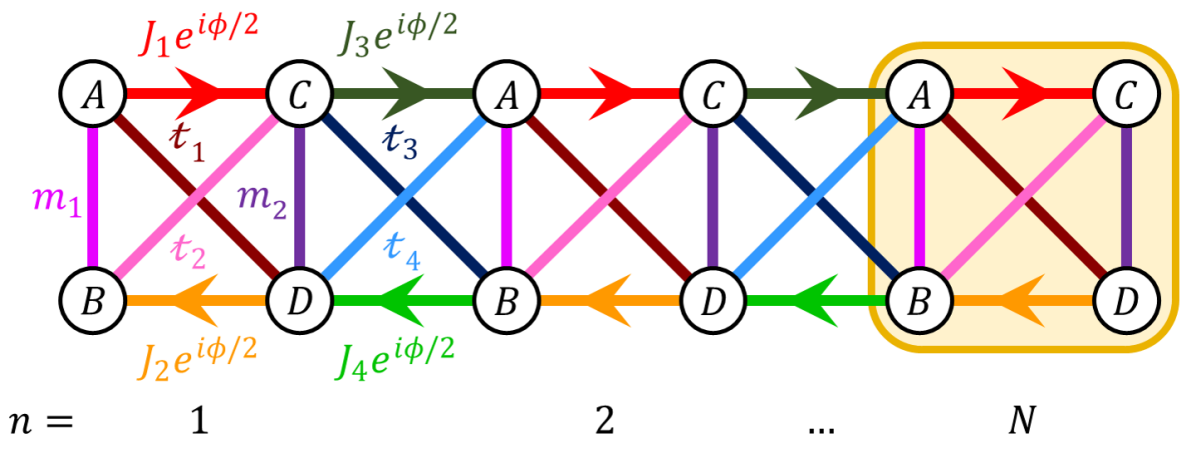
In this work, we consider a family of models closely related to the Creutz ladder, which will also include the alternating hopping amplitudes of the SSH model. Therefore, we will refer to them as CSSH ladders. To label each site, we will use the unit cell number and the internal coordinate , as indicated in Fig. 1. We will also use the nomenclature , , , . The general Hamiltonian for these models is (see Fig. 1):
| (1) |
where and are the floor and ceiling functions, and for . The operator destroys (creates) a particle in site . Our work is applicable to both bosons and spinless (or spin-polarized) fermions. The upper limits of the sums have been chosen to take into account the possibility of a finite system with an odd length , in which the last unit cell is not complete. When not explicitly noted otherwise, we will assume that is even, and then , the total number of unit cells. We consider the same phase shift in every horizontal link, implementing a magnetic flux of through each square plaquette, where is the charge of the particle.
We will also fix the vertical hopping amplitudes as equal, . This leaves 10 degrees of freedom, . Under periodic boundary conditions, this Hamiltonian can be rewritten as , where the first operator acts on the spatial coordinate (that is, the unit cell number ), while the matrix acts on the internal degree of freedom . The quasimomentum takes values along the first Brillouin zone. The bulk Hamiltonian has the form:
| (2) |
and will allow us to probe the topology of the systems in Section 4.
Out of all possible systems, we analyze particular cases in which the horizontal and diagonal hoppings, and , take two different values, and , in the spirit of the SSH model. In addition, we will focus our attention on cases where all energy bands are non-dispersive due to AB caging when and . The CSSH models will have, in general, 4 different bands, given that their unit cell consists of 4 sites. In addition to the Creutz ladder [Fig. 2 (a)], where , three different kinds of CSSH ladders that exhibit this behavior are:
-
•
The hourglass () CSSH ladder, with , [Fig. 2 (c)].
-
•
The rhomboid () CSSH ladder, with , [Fig. 2 (d)].
-
•
The delta () CSSH ladder, with , [Fig. 2 (e)].
The name for each kind of ladder comes from the shape formed by the links of the same value. We will parametrize and in the following way:
| (3) |
with . Thus, the Hamiltonian for any of the CSSH ladders is completely determined by the hopping amplitudes and , the angle and the magnetic flux phase . Unless specified otherwise111Some properties of the models, like the winding number or the chirality of the zero modes, are periodic in with period , not . This is related to the fact that the smallest closed loop in the model is a triangle with a flux of . However, most features explored in this work have a period of ., all values of are to be taken modulo . From this point on, we set and we consider , which sets the energy scale of the system but has no other effect in the dynamics. As we will see below, the CSSH ladders inherit some features from the Creutz ladder, and some others from the SSH chain.
These three models have not been previously studied in the literature, although they bear some relation to other quasi-1D insulators. The -CSSH ladder, when either or are zero, reduces to the orthogonal dimer chain [Fig. 2 (f)], a topological model that is usually studied as a chain of interacting spins [44, 45, 46, 47, 48, 49, 50, 51, 52]. The -CSSH ladder model connects the topological phases of the orthogonal dimer chain and of the -flux Creutz ladder in an adiabatic way, without losing the topological protection of the edge states at any point222In this regard, this model is similar to the - lattice, a non-topological 2D model with a flat band and two different tunneling amplitudes, which interpolates between the honeycomb lattice and the lattice [116, 117, 118]..
The spin- SSH chain with spin-orbit interaction [53, 54, 55, 56] is similar to the hourglass CSSH ladder in a certain regime, except for the distribution of magnetic fluxes. The hourglass-CSSH ladder with , in its trivial phase, also has the same geometry as certain compounds with XCl, Br [57]; and has been analyzed as a chain of interacting spins [58, 57]. Other models similar to the CSSH ladders, but with some missing tunneling amplitudes, have been studied, like the SSH ladder [59, 60, 9, 61, 62], the SSH bowtie ladder [10, 63] or the chequerboard chain [64]. A thorough exploration of other topological ladders can be found in [10].
3 Topology in simple models
The three main symmetries that are usually considered in the context of topology are particle-hole (PH) symmetry () and time-reversal (TR) symmetry (), which are both antiunitary, and chiral or sublattice symmetry (), which is unitary. They satisfy:
| (4) | |||
| (5) | |||
| (6) |
Their presence and type define the well-known symmetry classes in the periodic table of topological insulators [1, 65, 66], some of which can have topological phases, depending on their spatial dimension. The five topological classes in 1D can be consulted in Table 1.
In this paper, we follow the approach of considering the requirements (4-6) as the defining property of the three symmetries, which is a useful point of view for the analysis of topological insulators and has been used extensively in the literature [39, 67, 11, 16, 68, 69]. However, it is important to note that the particle-hole symmetries we discuss do not have the same implications as in a topological superconductor. Specifically, it does not imply the presence of Majorana end modes in the topological phases. The unit cells in the models we discuss are composed of more than one particle mode, and so their end modes are never formed by half a fermionic mode [70, 39, 67, 71].
| Class | A | AIII | AI | BDI | D | DIII | AII | CII | C | CI |
| 1D T. Inv. | | | | | |
In this section, we will review the relevant symmetries of the SSH chain and Creutz ladder, including the hidden symmetries in the Creutz ladder, essential for the protection of the edge states. Then, we will describe the symmetries and topology of the three CSSH ladder models proposed in this work. All the cases we consider are represented in Table 2, in which the symmetry classes and invariants of the different models are detailed.
3.1 The SSH chain
The SSH chain [73] [Fig. 2 (b)] is a 1D chain with two sites per unit cell, and , with a intracell tunneling amplitude of , and an intercell amplitude of , in which particles move around. Its Hamiltonian is:
| (7) |
where destroys (creates) a particle in unit cell number and sublattice .
This Hamiltonian has particle-hole (), time-reversal () and chiral () symmetries, where is complex conjugation. The matrices act on the internal degree of freedom, the subindex refers to the SSH chain, and the superindex indicates the matrices are . The model belongs to class BDI [42, 1], and so it can be characterized by its Zak phase (for a more detailed discussion, please refer to Appendix A). The Zak phase of a given band is given by333As detailed in Appendix A, there are two slightly different quantities that have been called “Zak phase” in the literature. We follow the convention in [42], which is tied to the choice of the so-called Basis I for tight-binding models [99].:
| (8) |
where is the -th eigenstate of the bulk Hamiltonian of the system [74].
The internal states of the SSH chain and have positive and negative chirality, respectively, corresponding to the two sublattices. The bulk states have equal support on both sublattices, while the topological edge states, when present, only have support on one of them. This is a general phenomenon in chiral-symmetric topological phases. The SSH chain is topological whenever , giving rise to one chiral zero mode in each end of the chain, protected by the chiral and PH symmetries [75].
3.2 The Creutz ladder
3.2.1
The Creutz ladder Hamiltonian can be obtained from equation (1) setting . Its unit cell is formed by the upper and lower sites, and , of each rung. The system is metallic when or . When , the system belongs to class BDI, with the symmetries , and [38, 34, 68], where the subindex refers to the Creutz ladder. This TR symmetry, as well as several others that we describe below, is non-conventional, but it behaves exactly like a usual TR symmetry for topological considerations, so we will consider it as such. For a more detailed discussion, see Appendix B.
The topology of the model can be characterized by the Zak phase, which is if and vanishes otherwise; except if , where it is not defined because the system is metallic. These lines at constant in the phase diagram separate distinct topological phases, which can be distinguished by the chirality of their edge states or the sign of their winding number, [8, 12]. One protected chiral edge state appears in each end of the ladder when the system is topological.
The chiral basis is now, in the basis, , corresponding to the chirality of the left/right edge state. The edge states are protected by both the chiral and PH symmetries.
A unitary transformation [34] maps the ladder to the SSH chain, with and , as the topological phase transitions (TPTs) of each model suggest. For instance, this means that the rungless case (), when AB caging completely localizes the topological edge states of the Creutz ladder in the first and last rungs, corresponds to the fully dimerized limit () in the SSH chain, where the edge states are localized at the first and last sites. This has important consequences, as we discuss below. The mapping also relates the chiral bases of the models. This illustrates a key difference between them: the two chiral states in the SSH chain coincide with its sites, while those in the Creutz ladder do not. While one of the chiral states (and, thus, one of the end states, if they are present) can be easily eliminated in the SSH chain due to open boundary conditions, this is impossible in the Creutz ladder. Thus, the topology of the Creutz ladder does not depend on the choice of unit cell, unlike that of the SSH chain.
| SSH | BDI: [] | ||
|---|---|---|---|
| Creutz | |||
| Trivial | AI: NT [] | BDI: [] | |
| Trivial | BDIa: [ ] | BDI: [] | |
| -CSSH | |||
| AIb: NT [: ] | AI: NT [] | BDI: [] | |
| BDI: [: ] | BDI: [] | BDI: [: ] | |
| -CSSH | |||
| Trivial | AI: NT [] | BDI: [] | |
| Trivial | BDI: [, ,] | BDI: [: ] | |
| -CSSH | |||
| Trivial | A: NT [none] | D: [] | |
| Trivial | AIII: [] | BDI: [] | |
3.2.2
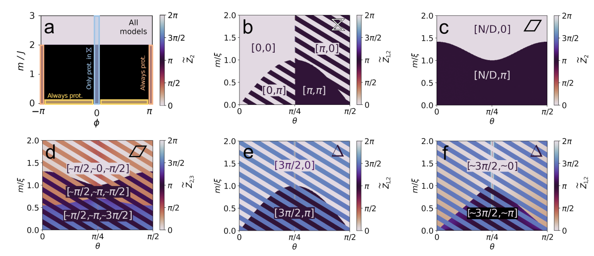
For other values of the magnetic flux, the TR symmetry holds but the PH and chiral symmetries break down. The edge states are only protected in the rungless case. When , the two edge states drift away from zero energy, given that the model belongs to class AI, with no protecting symmetries (see Table 2). The Zak phase is still quantized due to inversion symmetry [42], which also causes the end states to be degenerate in the thermodynamic limit. Thus, in this regime, the system is a topological crystalline insulator [8, 76]. However, in it, the end states are not topologically protected against any kind of disorder, given that any disorder will break inversion symmetry. The topological phase diagram of the Creutz ladder as a function of and is depicted in Fig. 3 (a), as well as the regions where topological protection will be found in the CSSH ladders: whenever or , like in the Creutz ladder, and, in the hourglass case, also when .
When , the topological protection can only be explained due to the presence of so-called “hidden symmetries”. These are symmetries that satisfy one of the conditions (4-6), but they act in a non-trivial way on the spatial degree of freedom, so they cannot be reduced to their effect on the inner space Hamiltonian [77]. They can determine the topology of the system, exactly like their conventional counterparts [78, 79, 80, 81, 82, 83, 84].
The topological protection when can be explained due to the presence of the hidden chiral symmetry , which reflects the fact that the lattice is bipartite, and the hidden PH symmetry . The subindex indicates this symmetry is analogous to the chiral symmetry in the SSH chain, while denotes that the operator is related to and . In the spatial basis of the full Hilbert space, they are represented by the operators:
| (9) | |||
| (10) |
where is the diagonal or block-diagonal matrix formed by the elements . In general, we will mark operators acting on the whole Hamiltonian with a tilde, and those that act on the inner space Hamiltonian with no tilde. These operators cannot be factorized to separate their effect on the inner and spatial subspaces, as is customary. These hidden symmetries place the rungless Creutz ladder in the BDI class (see Table 2). The operators and are related to the hidden symmetries and mentioned in Ref. [80] by the inversion symmetry of the ladder.
3.2.3 AB caging and topological protection
We want to bring attention to an important detail at this point, which is often overlooked. In most topological materials, if the system has a small size, the energies of the protected end modes have a finite (albeit small) value, due to their overlap. In the systems we study, these energies are at least one order of magnitude smaller than the gap, and so do not break the bulk-boundary correspondence. However, the zero modes in the rungless Creutz ladder are completely localized to the two end sites of the ladder, and this causes their overlap to vanish. This localization has the same nature as AB caging, as it is caused by destructive interference of the wavefunction due to the magnetic flux and connectivity of the ladder. Thus, the end modes are pinned at zero energy for any length of the ladder , including the one plaquette limit, . This interplay between AB localization and topology protects the zero modes even better than topology alone can, and allows the detection and use of protected states in systems with only a few sites. This also happens in the three CSSH ladders, where the edge states present a larger variety than in the Creutz case444The end states in the completely dimerized SSH chain also have zero energy for any length of the chain, as a trivial consequence of disconnecting the end sites from the rest of the chain. In the -flux Creutz and CSSH ladders, this phenomenon occurs while the end sites are connected to the rest of the system..
3.2.4
When , the Hamiltonian has a unitary commuting symmetry , that makes it decouple into two topologically trivial subspaces: a dispersive band spanned by , and a flat band at energy , spanned by . When , the states that form each subspace switch their roles, and the value of their energies is reversed (for instance, the flat band is located at ).
4 Topology of the CSSH ladders
We will now analyze the three CSSH models. They have topological phases with protected zero modes if (-flux regime) or (rungless regime). Additional constraints must be satisfied for each model to be topological, something we explore below using their topological phase diagrams (Fig. 3). The coexistence of the symmetries from the -flux and rungless regimes causes the case to be block-diagonalizable in the -CSSH and -CSSH ladders, revealing a trivial and a topological subspace. The -CSSH ladder is also topological in the case, while the other two models are not. In the chiral models, two different nontrivial phases appear with edge modes of opposite chirality and winding number, in the same way than in the Creutz ladder [8, 12]. These phases are separated by two topological phase transitions at . For more details on the relevant topological invariants, please refer to Appendix A.
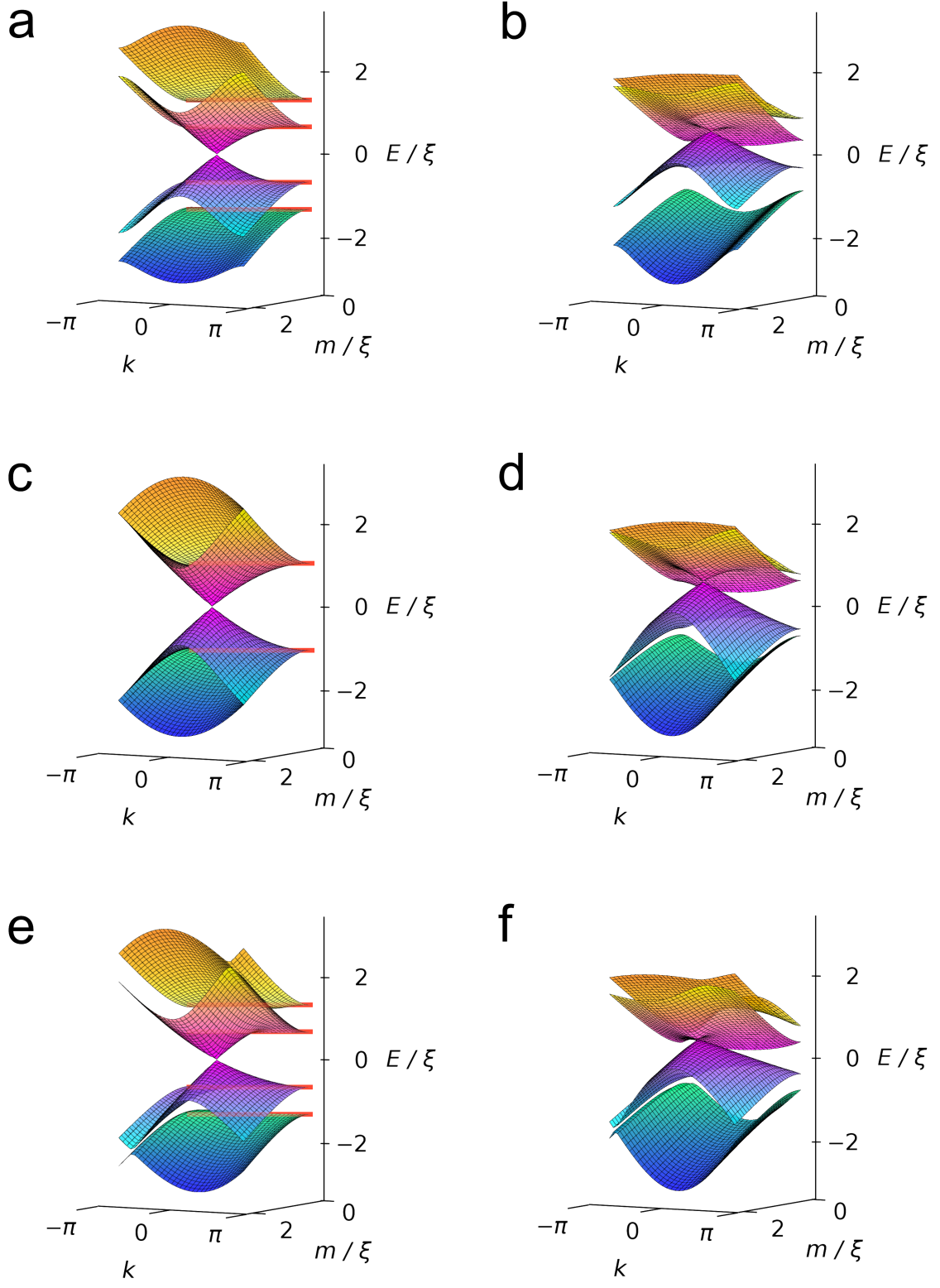
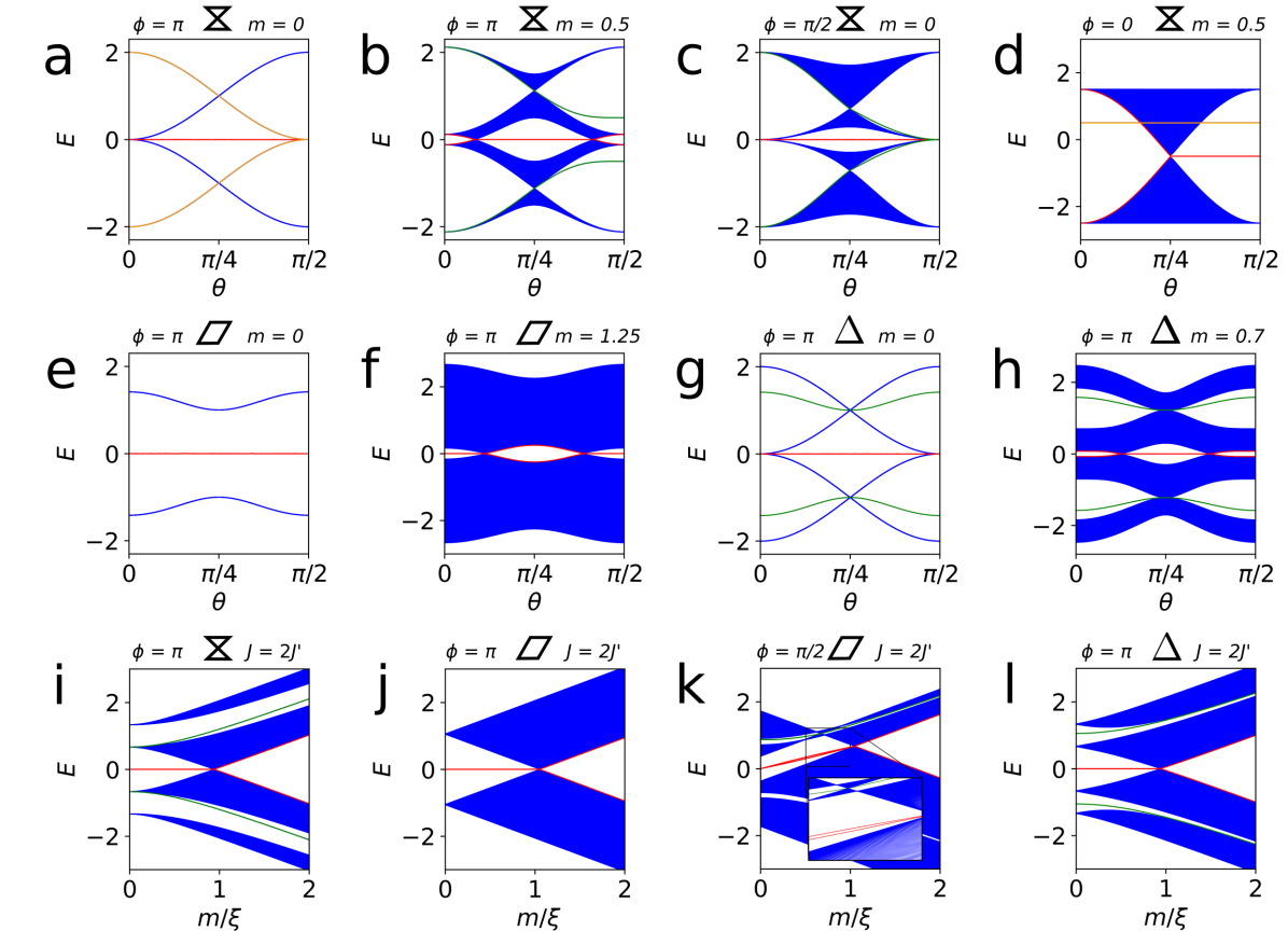
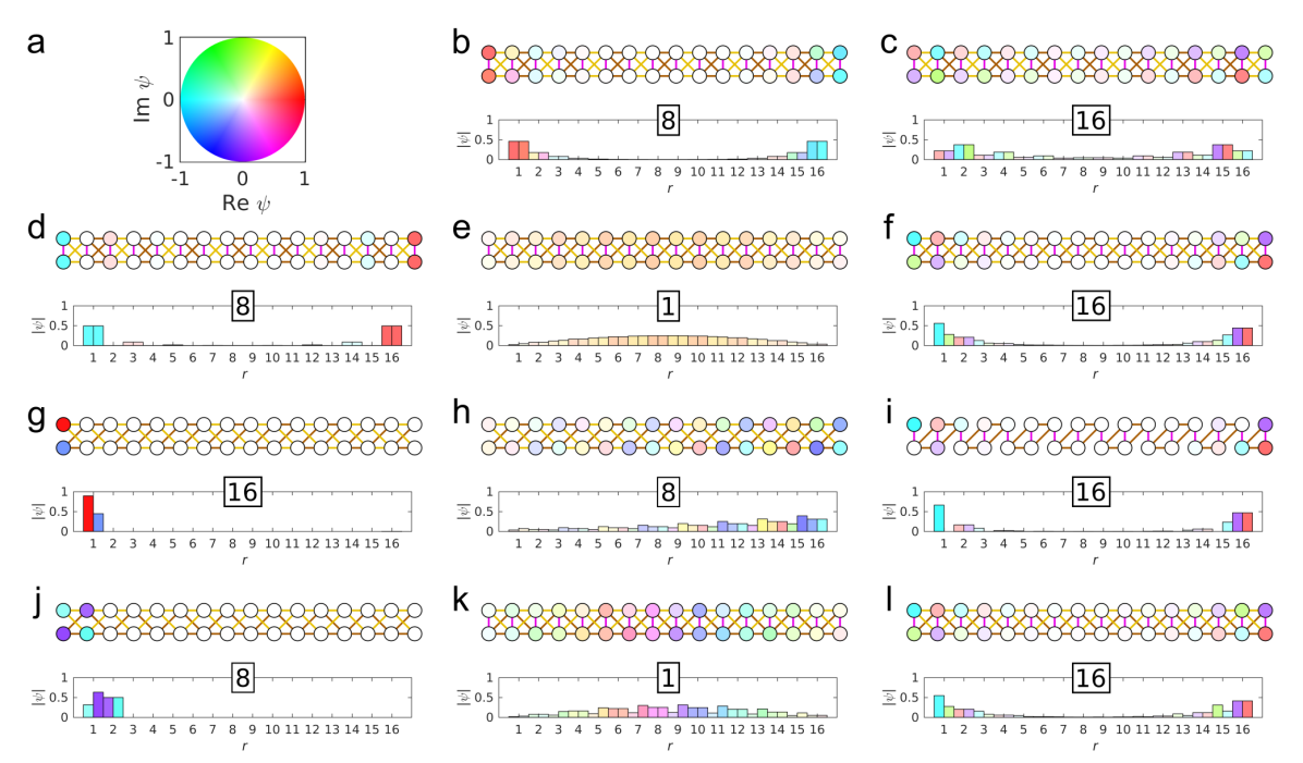
The different topological classes, symmetries and invariants of the SSH, Creutz and CSSH systems for every combination of parameters can be found in Table 2. The detailed list with the analytical expression of all symmetry operators is reserved for Appendix B, although the most relevant ones will be mentioned in the text. The bulk bands for the different models, depicted in Fig. 4, reflect the presence of these symmetries. The spectra for the finite ladders, with different types of topological end modes, is also studied below (Fig. 5). Finally, the spatial distribution of some energy eigenstates of different 32-site ladders are represented in Fig. 6. Each of the aforementioned figures is referenced below, in the context of the different models. In all cases, the energy scale has been fixed by setting .
4.1 The hourglass CSSH ladder
4.1.1
In this case, the -CSSH ladder [see Fig. 2 (c)] belongs to class BDI, with symmetries , and , which are equivalent to the Creutz ladder symmetries in the same regime, and have dimension 4 (the superindex was omitted in all matrices for clarity). This is reflected on the symmetric form of its spectrum [see Fig. 4 (a)].
In the rungless -flux case, the system has four flat bands and a commuting unitary symmetry . This kind of symmetry allows us to block-diagonalize the Hamiltonian, and study the topology of the different subspaces independently. In this case, the system can be mapped into two independent, fully dimerized SSH chains, a trivial and a topological one, with amplitudes , and , . They correspond, respectively, to the flat bands with energies and [see Fig. 5 (a)]. The -CSSH ladder end modes correspond to the edge states of the topological chain. When is switched on, it couples the two chains and the symmetry breaks.
In the case, the full four-band system must be considered. The topological invariant related to the boundary states that appear in a particular gap in the system can be obtained as the sum of the Zak phases of all the bands below it [85], . In a topological symmetry class, the number of topological edge states per end in that gap will be [86, 85, 87, 88]. When quantized, the topological invariants associated with the first and third gaps of all CSSH ladders have the same value, , so to identify different phases we will use .
The topological phase diagram for this regime is depicted in Fig. 3 (b). The first invariant, , behaves like the one in the SSH chain, being topological when . The second one, , is topological when . When , this condition is reduced to the one in the Creutz ladder. The states in the second (or central) gap are protected by the chiral and PH symmetries in the topological phase [see Fig. 5 (i)]. Those in the first and third gaps only appear when , and thus satisfy the bulk-boundary correspondence. However, they are not pinned in the middle of their gaps, as can be seen in Fig. 5 (b). This is because the symmetries of the system can only protect states in the middle gap, given that they only guarantee a symmetric spectrum about zero energy. This is further explained in Appendix E. They do guarantee, however, that the states in the first gap have the opposite energy to those in the third gap. These states can be described as topological, but not protected. If , the system has six topological edge states, two of which are protected at zero energy. In Fig. 6 (b,c), the edge states in the first and second gap of the system are shown.
4.1.2
For these values of the magnetic field, the TR symmetry still holds, but the other two break down, in a similar situation to that of the Creutz ladder. This can be appreciated in Fig. 4 (b). If , the model is a topological crystalline insulator in class AI. Its states are not topologically protected against disorder, but they are still degenerate in a long enough ladder due to spatial inversion.
When , the same chiral and PH symmetries as in the Creutz ladder appear. However, they are not hidden anymore, because the unit cell of the system is larger now. Their operators on the bulk Hamiltonian are and . As noted earlier, the subindex indicates this symmetry is analogous to the chiral symmetry in the SSH chain. In this regime, only when , and always holds. Like in the case, only the states in the middle gap are protected [see Fig. 5 (c)]. Their exact form is described in Appendix C. The Zak phases take the same values as in the -flux regime [Fig. 3 (b)].
4.1.3
If the magnetic field is turned off in the -CSSH ladder, the topology inherited from the Creutz ladder disappears, but not the one generated by the staggered, SSH-like amplitudes. In this case, the bulk Hamiltonian has a unitary commuting symmetry, , that generates two independent subspaces, exactly like in the Creutz case. One of them is a topologically trivial doubly degenerate flat band at energy , spanned by the internal states and . This subspace can be turned into two non-degenerate flat bands if the vertical hopping amplitudes are set to different values in (1).
The other subspace is now analogous to an SSH chain with amplitudes , which will be topological if , in contrast to the Creutz case, where the system is metallic at . Its spectrum is pictured in Fig. 5 (d). The vertical amplitude behaves like a homogeneous chemical potential, shifting the SSH chain spectrum downwards, but having no other effect in the topology. The topological chiral end states are analogous to those in the SSH chain, with the left (right) state only supported on the odd (even) sites, as can be seen in Fig. 6 (d) for the , system.
4.2 The rhomboid CSSH ladder
4.2.1
When , the -CSSH ladder [see Fig. 2 (d)] is in class BDI, with the symmetries
| (11) | |||
| (12) | |||
| (13) |
where
| (14) | |||
| (15) |
The angles and are related by the expression:
| (16) |
The first and third gaps are closed at , forming two Dirac cones [see Fig. 4 (c)], and this renders and not meaningful, as only the middle gap exists. The ground state of the system lies at , something apparent in Fig. 6 (e) for , . The relevant phase diagram is shown in Fig. 3 (c). The system is topological when . When that condition is met, the gap has zero modes, protected by the chiral and PH symmetries. Their form for , is depicted in Fig. 6 (f), and they can be seen in its spectra as a function of , in Fig. 5 (f), and as a function of , in Fig. 5 (j).
The chiral symmetry of the system , which protects the end modes along with , depends on . It interpolates between a Creutz-like chiral symmetry, at , and its counterpart in the orthogonal dimer chain, at . This provides a degree of freedom to choose the system in which the protecting symmetries will be less broken in a particular implementation. The Creutz ladder chiral symmetry can withstand a broader range of on-site disorder configurations without breaking than that in the orthogonal dimer chain (see Appendix B for a more detailed discussion). On the other hand, the orthogonal dimer chain is a simpler model, and can therefore have less sources of disorder than the Creutz ladder, so it might be preferable for some applications.
As can be seen in Fig. 3 (c), when or vanish, the system can still be topological, unlike the other models. The resulting lattice is the orthogonal dimer chain, depicted in Fig. 2 (f). It is topological when and (assuming ). As mentioned above, this model is usually studied in the context of interacting spins [45, 47, 48, 50, 52]. The -CSSH ladder connects the topological phases of the Creutz ladder (obtained when ) and the orthogonal dimer chain (), two previously unrelated models. The superposition of both topological edge states in the orthogonal dimer chain with is shown in Fig. 6 (i).
Furthermore, when and (for any value of ), the system has a unitary commuting symmetry that creates two subspaces that can be mapped to two fully dimerized SSH chains, with amplitudes . They are topological and trivial, respectively. The complex amplitudes, corresponding to a magnetic potential in the direction of the chain, do not affect the topology, and only modify the form of the PH and TR operators of the SSH chain. The topological subspace has two protected zero modes. The upper and lower bands of the two SSH chains are degenerate, with energies . However, given that their states never mix, there is no need to resort to the non-abelian topological invariant [67]. The spectrum of the system is pictured in Fig. 5 (e).
4.2.2
The system is still TR-symmetric for these values of [see Fig. 4 (d)], but the form of the TR operator is now more complicated (see equation (43) in Appendix B). When , the chiral symmetry pins the edge states in the middle gap exactly at zero energy. The left zero mode is depicted in Fig. 6 (g) for , . A PH symmetry, (see Appendix B), is also present there. Therefore, the case belongs to the BDI class, while the system belongs to class AI, which is not topological.
To understand the topological phase diagram, we need to keep in mind that the Zak phase is only guaranteed to be quantized if the system with periodic boundary conditions is symmetric under a spatial inversion operation that leaves the point at the center of the unit cell invariant [84]. The -CSSH ladder is symmetric under a specific spatial inversion symmetry, in which the inversion center is located between the and sites (see Appendix B for a matrix representation).
In this regime, the invariants associated with the first and third gaps are no longer equal. In fact, one of them has a topological phase transition between non-quantized values, while the other one does not. Only presents a phase transition if , and only presents one otherwise. This can be seen in Fig. 3 (d). Non-protected end states appear in the first and third gaps, and they do not follow the usual bulk-boundary correspondence. One of these end states is pictured in Fig. 6 (h). The topological phase transitions are related to gap closings in the spectrum that do not change the number of end states [see the insert in 5 (k)], but do change the end (left or right) in which they appear. We discuss these states in depth in Section 4.4.
In the -CSSH ladder, the Zak phase is quantized whenever the system belongs to a topological class, except for and in the case. There, is equal to , indicating the presence of topological zero modes. Additionally, the second gap end states in a ladder with an even number of rungs are not related by spatial inversion, and so they are not degenerate, even in a large system. This occurs because the open system loses its global inversion symmetry, and its effects can be seen in the corresponding spectrum as a function of in Fig. 5 (k).
4.2.3 Edge state tunability
To show an application of the high tunability of the protected edge states, let us consider the left topological zero mode of the rungless -CSSH ladder [see Fig. 6 (g)]:
| (17) |
The dependence on and of the zero modes provides a topologically protected method to control a particle located in the two end sites, by changing the parameters of the system.
We can establish any state in the Bloch sphere, with controlling the weight of each site and controlling their relative phase. To obtain a given state with , the following parameters must be chosen:
| (18) | |||
| (19) |
such that , . In the cases of (), the system becomes topologically trivial. The states defined by expression (17), however, are still eigenvalues of the model, and become part of a flat band instead of being topological zero modes.
In particular, the system can be initiated with the particle in eigenstate in the model with and , and then turning on adiabatically until the condition is reached. In particular, this allows us to prepare the topological end modes of the Creutz ladder, by choosing . As long as the chiral symmetry of the system, , is not broken, this protocol is topologically protected against disorder, even in small systems. The left state in the -CSSH ladder can also be used, with the same results. For more information, refer to Appendix C, where we discuss the caged zero modes of all models.
4.2.4
In this regime, the system is topologically trivial. When , a doubly degenerate flat band appears at , and one dispersive band is located at each side of it, touching it if . When is turned on, a flat band remains at , spanned by , and the other three are dispersive.
4.3 The delta CSSH ladder
4.3.1
When , this -flux model, in contrast with all the previous ones, does not have TR and chiral symmetries inherited from the Creutz ladder, and only has its PH symmetry, . This is related to the fact that one of the legs is formed by strong links, and the other one by weak ones [see Fig. 2 (e)]. Given that the TR symmetry in Creutz-related ladders swaps the two legs, this imbalance breaks TR symmetry. The effects of this symmetry breaking can be easily seen in its spectrum [Fig. 4 (e)], which is symmetric about the origin , but not in or in . The first and third gaps are narrowest at opposite values of , and not in as in the other ladders.
Therefore, the -CSSH ladder with and belongs to the D class. Other instances of 1D or quasi-1D topological D-class materials are typically superconducting systems. Its topology is characterized by a invariant, which in the 1D D class coincides with the Zak phase555Its value for the middle gap can also be calculated using the Pfaffian of the Hamiltonian. This has been confirmed numerically to coincide with in the -CSSH ladder. [39, 89]. As depicted in Fig. 3 (e), takes a constant value of , except in the Creutz limit , where it becomes undefined. On the other hand, indicates that protected zero modes will appear if . These states are represented in Fig. 6 (k,l) for and . They are only protected by PH symmetry, as there is no chiral symmetry in the system.
Additionally, non-protected edge states located in the left end of the ladder appear in the first and third gaps. They can be seen in the spectrum in Fig. 5 (g,h,l). One state of this kind in the flat band case is depicted in Fig. 6 (j). Interestingly, these states do not follow the usual bulk-boundary correspondence, and can be related instead to a Chern number. We discuss these states in detail in subsection 4.4, and in Appendix D.
As usual, when and , the bands flatten and the chiral and TR symmetries and appear (see Appendix B). The model is BDI and topological (). The end states of the system are now totally localized to two sites due to AB caging.
4.3.2
In the case, the model has no relevant symmetries [see Fig. 4 (f)] and belongs to class A, not topologically protected in 1D. The second gap end modes are not degenerate even in the even-runged, large chain case, because the boundaries of the system break spatial inversion. In this case, , so we only represent in the phase diagram [Fig. 3 (f)].
When , the chiral symmetry puts the system in class AIII and makes the system topological, with and , and hosts a pair of protected zero modes in the middle gap (see Appendix C). Like their -CSSH counterparts, these states are localized in only two sites, and they can be tuned in the same way as them. Non-protected states of the same nature as in the -flux can also appear, see the next subsection for details. There are other known ways to achieve AIII TIs with the geometry of the Creutz ladder: to include an energy imbalance between the legs [11], or additional complex hopping amplitudes in the diagonal or vertical tunneling amplitudes [10, 12, 13]. As we have seen, by changing its parameters, the -CSSH ladder can belong to three of the five topological classes in 1D (see Table 1). The end modes remain protected when changing from one class to another.
The Zak phase is not always quantized in the -CSSH ladder because, like the -CSSH case, it is only invariant under a specific kind of generalized inversion symmetry. This transformation only flips the longitudinal coordinate of the ladder (see Appendix B). The value of is quantized when the system belongs to a topological symmetry class, but not , as we discuss in Section 4.4.
4.3.3
The system is topologically trivial. Like in the other models, a doubly degenerate flat band appears in in the rungless regime. The other two bands are dispersive and touch the flat band for all values of , making the system metallic. Like in the -CSSH case, when is switched on, a non-degenerate flat band spanned by lies at , while the rest of the bands become dispersive.
4.4 Non-protected states and Chern numbers
In the rhomboid and delta CSSH ladders, a single edge state can be found in the first or in the third gaps, and they often appear in both at the same time. These states, when present, are both localized at the same side of the ladder, not one at each side. They can be found at the left or right ends in the -CSSH ladder, and only at the left end in the -CSSH ladder. These states are not protected, as they are not located in the central gap (see Appendix E for details), and they do not follow the usual bulk-boundary correspondence, as they appear even though takes intermediate values between and [see Fig. 3 (d,e,f)]. However, they have a topological nature, given that they appear due to a topological obstruction that can be understood by exploring the Wannier functions of the model. For a detailed analysis, please refer to Appendix D.
Interestingly, this kind of edge states have been recently reported in a recent paper [41] in trimer chain models with no inversion symmetry. In said work, it is argued that these edge states, even though they exist in a 1D model, are related to the 2D Chern number associated to the model changing along a closed path in its space of parameters. This is associated with the topological pumping that would happen if the model was physically changed in time following the chosen path [41, 90].
In the CSSH ladders, an analogous invariant can be found, if we consider an appropriate extension of the models. In the -CSSH ladder, the relevant path along parameter space can be chosen as [see Fig. 7 (a)]:
| (20) |
where , , is the parameter along the path, are the diagonal hopping amplitudes in Hamiltonian (1). The rest of the hopping amplitudes are constant along the path. For the -CSSH ladder, the value of and must be interchanged.
For , the system is a - or -CSSH ladder as defined in Section 2. In the opposite point of the path, , the system is the result of reflecting said ladder along the horizontal axis, and thus the value of its Zak phase will be the opposite. This system will have non-protected end modes on the opposite side to the non-reflected version. As an example, the different models visited along the path in the delta case are depicted in Fig. 7 (b).
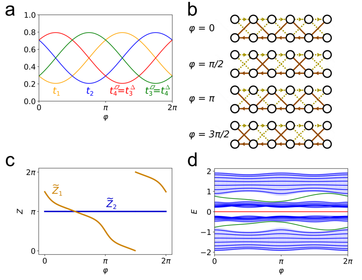
For the -CSSH ladders, the PH symmetry must be broken at some points to avoid band degeneracies along the path, and so in that case we also consider a changing , for instance:
| (21) |
Thus, , and the degeneracies that otherwise appear at are avoided. In the rhomboid case, the first and third gaps of the -flux systems close, so the invariant loses meaning there.
As the system changes along the path, the Zak phase of the first band starts increasing or decreasing, and eventually wraps around and returns to its initial value. This winding of the Zak phase indicates that the lowest band has a nontrivial Chern number as it changes along the path. In the -CSSH ladder, when . We can see this for in Fig. 7 (c), where . The second gap has an invariant of , which predicts no edge states of this kind there (the states in this gap are related to the usual Zak phase instead). Equivalently, the value of along the path does not wrap around, and instead remains constant [see Fig. 7 (c)]. The value of is nontrivial, indicating the possible existence of an edge state in the third gap.
It is important to note that invariant is associated with the whole path, not just the particular system we are interested in. For this reason, the bulk-boundary correspondence is only guaranteed to be satisfied when considering the entire path, not at a single point in it. The value of the Chern number cannot predict if the end states in the CSSH ladders will appear in the gaps or not, it only indicates that a single state can appear in each gap. Its sign also has a physical meaning: it indicates the direction of pumping of the end modes if the system is changed along the path. The Zak phase itself, however, is not without meaning. A value of around () indicates the edge states in the first gap will appear in the right (left) end of the ladder, due to its relation to the Wannier centers, as explained in Appendix D.
The situation is completely analogous to the trimer chain case [41]. In Fig. 7 (d), the spectrum with periodic (light blue background) and open boundary conditions (lines) for the -CSSH ladder in subfigure (c) is represented along the path, for . We can appreciate the non-protected end states, in green, moving around in their gaps, as dictated by their Chern number. The protected end states in the central gap, in red, stay constant at zero energy, as their Zak phase of dictates.
In the -CSSH ladder, and are also nontrivial, while . As discussed in Section 4.2.1, one of the two outer gaps undergoes a topological phase transition as increases [see Fig. 3 (d)], across which the Zak phase jumps discretely but the number of end states remains constant. The end of the ladder in which the end state is located changes accordingly, from the right to the left end. This is accompanied by a change in the Chern number associated with that gap. If , if , where no phase transition is present in the first gap. For other values of , changes from to as increases and transverses its critical value. All signs are reversed if . The behavior of is completely analogous, but the phase transitions are now only present if , and all signs are reversed.
4.5 CSSH ladders with an odd number of rungs
The discussion above assumes systems with an even number of rungs, that is, an integer number of unit cells. We now briefly discuss now the case when the number of rungs is odd. This means half a unit cell is left unpaired, either in the left or the right end of the ladder. If this choice of boundaries broke the protecting symmetries, the central gap edge states would not be protected anymore. However, all the chiral symmetries of the systems are preserved under this choice of boundaries, implying that, when present, the edge states in the middle gap will be chiral and protected. In the cases where the topology is protected by or , the states appear in the half unit cell when expected, and in the - and -CSSH ladders they take an analogous form to their counterparts on the other end, something that is not true in the even-runged ladders. This is a consequence of the presence of a global inversion symmetry, which will make the left and right states degenerate in the thermodynamic limit, even in the , case.
In the cases where the topology is protected by , the SSH-like chiral operator, topological states appear in the half unit cell when the Zak phase is trivial, and no states appear when it is topological. This is a well-known phenomenon in the SSH chain [91, 43, 3], and can be easily understood in terms of the lattice geometry. In the D-class topological -CSSH, the states are protected by the PH symmetry , which is not broken either in odd-runged ladders, and zero modes appear in the half unit cells. For a discussion of the states in even and odd-runged ladders, see Appendix C.
Finally, the non-protected states in the first and third gaps of the - and -CSSH ladders can also appear or disappear in the same way as SSH-type zero modes. Depending on the choice of boundaries, both left and right non-protected modes can be found in both ladders at the same time.
5 Experimental implementations
Our work considers the single-particle case only, and so it is applicable for both bosonic and fermionic particles. As mentioned above, the Creutz ladder has been implemented in a cold atom system using orbital-momentum coupling [92, 93] and can be simulated in a specific regime [27] in a rhombus chain photonic lattice [27, 28, 29]. Recently, a Creutz ladder plaquette was also implemented in a superconducting system [94]. Some other theoretical proposals have been made to implement the Creutz ladder in cold atom systems, either by using two hyperfine states as the legs of the ladder [11] or two zigzag chains [12]. A system of helical coupled-resonator waveguides [95] also produces the Creutz ladder as an effective model. By changing the tunneling amplitudes in the appropriate way, something particularly tunable in the mentioned systems, these setups can be employed to implement the CSSH ladders, under certain constraints. The easiest model to implement is probably the -CSSH ladder, given that the staggering of its amplitudes follows a simple SSH-like pattern.
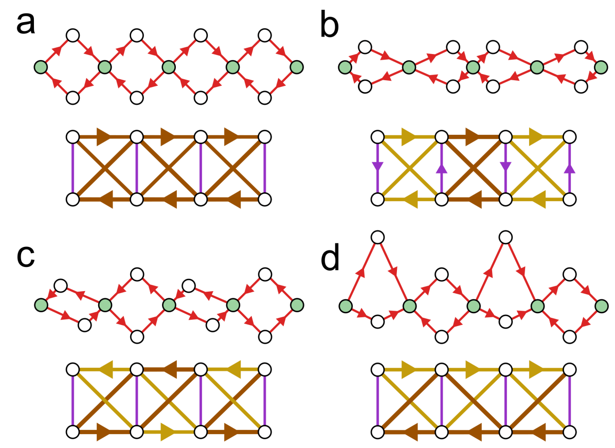
Modified rhombus chains with a large chemical potential in its central sites can be used to implement the three CSSH models, following the Creutz ladder implementation presented in [27]. Their geometries are represented in Fig. 8. The -flux case can be obtained directly, but the and degrees of freedom are not independent, and that restricts the regimes that can be obtained. For a detailed explanation and the relevant effective Hamiltonians, refer to Appendix F. This general scheme can be used to implement the CSSH ladders in a photonic lattice or other systems, like ultracold atoms or superconducting circuits.
In particular, the tunneling amplitudes in cold atom implementations [12, 11, 92, 93] are related to the intensity of the lasers that induce the Raman-assisted transitions. This provides an easy way to independently tune each amplitude and obtain any of the CSSH ladders. In some proposals, like for instance [12], the and parameters can be tuned independently, and this would allow for the implementation of the D class TI or the rungless topological phase with any .
Four-site versions () of all CSSH models can be implemented in the superconducting system in [94], by changing the appropriate tunneling amplitudes. It is worth noting that, in this limit, the -CSSH ladder reduces to a Creutz-style plaquette (which, in turn, can be rearranged as a square plaquette with a magnetic flux of ), and the and -CSSH ladders become identical to each other. These systems, although small, still have states at exactly zero energy, which are protected by the same symmetries as those in the longer models.
The complex hopping amplitudes, which constitute one of the main difficulties in implementing these models, a periodic on-site energy driving in a waveguide lattice [27], and it appears naturally as a result of the two-photon transition in the cold atom implementation [93], and of the pump that couples the modes in the superconducting scheme [94].
Additionally, given that the fermionic Creutz model is equivalent to a spin- particle hopping in a chain of sites in a specific gauge field [80, 11, 96], different fermionic implementations could also be considered for both the Creutz and the CSSH ladders, including fermionic cold atoms, semiconducting quantum dots or trapped ions, provided that the appropriate gauge field and different tunneling amplitudes and spin-orbit couplings can be established.
6 Conclusions
In this work, we propose and analyze a family of quasi-1D topological insulators, the CSSH ladders, with rich topological phase diagrams and flat-band regimes due to Aharonov-Bohm caging. Each of the models has some peculiar properties. The hourglass CSSH ladder can exhibit Creutz-like and SSH-like topological zero modes. The latter arise in the absence of a magnetic field, in contrast with the Creutz ladder case, where the model is trivial. The rhomboid CSSH ladder has a tunable chiral symmetry, which can be used to predict which will be the best quasi-1D model to use in each experimental setup to increase the protection against disorder. And, finally, the -flux delta CSSH ladder is a quasi-1D topological material in the D class with no superconducting term, something rather unusual. By changing its parameters, this topological phase can be adiabatically connected with a BDI (,) and an AIII phase (,), without losing the protection of the edge states. This can be of interest to explore the differences between 1D topological symmetry classes in a simple model.
The wide variety of topological states presented here are also tunable by changing the , or parameters, which provides a high degree of control. They also have the robustness implicit to topological protection, which is still present in small, experimentally accessible systems in the rungless case. For these reasons, they are highly suitable to be used in the fields of quantum information and computation. For instance, they could be used in a quantum memory, as part of a symmetry-protected qubit architecture, or as a means of transferring particles or states between the two ends of the ladder in a robust way. Additionally, the topological end modes in the rungless CSSH ladders are pinned at exactly zero energy, even for ladders only a few sites long, thanks to AB localization. This feature is inherited from the Creutz ladder, and makes a wide variety of topologically protected zero modes experimentally available, even in small systems. An interesting follow-up to this research would be to explore the potential of these topological zero modes in different quantum information tasks, and compare them to other topological systems. Other intriguing topic is the study of the non-protected states in the rhomboid and delta CSSH ladder, which do not follow the bulk-boundary correspondence and are instead related to a Chern number. Previously reported on the trimer chain, they are reminiscent of topological states in quasicrystals. Their generalization to higher dimensions may be a promising topic for future research. Finally, the applications of the wide variety of topological pumps that are possible in these models, some of them present in the Creutz ladder [12] and others in the trimer chain [90], also constitute an interesting subject to explore further.
Finally, we propose a setup to implement the CSSH ladders in a photonic lattice system as an effective low-energy model in three modified rhombus chains. The large number of flat-band systems recently implemented in this kind of environment show that these lattices can be realized with the current technology. Given that our study applies to both bosons and fermions, the CSSH ladders can be realized in many other platforms, such as cold atoms, semiconducting quantum dots or superconducting circuits.
Acknowledgements
We would like to thank Álvaro Gómez-León and Luca Leonforte for fruitful discussions. C. E. Creffield was supported by Spain’s MINECO through Grant No. FIS2017-84368-P. G. Platero and J. Zurita were supported by Spain’s MINECO through Grants No. MAT2017- 86717-P and PID2020-117787GB-I00 and by CSIC Research Platform PTI-001. J. Zurita recognizes the FPU program FPU19/03575.
Appendix A Topological invariants
To probe the topology of the CSSH ladders, we have used the Zak phase, calculated numerically using bulk Hamiltonian (2). In this Appendix, we specify some additional details about this calculation, which are not often discussed in the literature.
In the strong topological insulator phases of the models (that is, when or ), they belong to the symmetry classes BDI, AIII and D, which can harbour topological phases in 1D. The topological invariant in classes BDI and AIII is the winding number , of type . In class D, the invariant, , is related to the Pfaffian of the bulk Hamiltonian, of type .
However, these topological invariants satisfy the following relations to the Zak phase [12, 10, 39, 89]:
| (22) | |||
| (23) |
provided spatial inversion symmetry is present and the center of the unit cell is chosen as the origin of coordinates.
Even in the cases where inversion symmetry is not present, the Zak phase is still a good topological invariant for protected zero modes, as we explain in the main text, and can also give us information about the non-conventional end states, related to a Chern number instead, that appear in the - and -CSSH ladders (see subsection 4.4 and Appendix D).
In the CSSH ladders, two distinct nontrivial phases appear, with , corresponding to and respectively, taken . These two phases cannot be distinguished with the Zak phase alone. They can be characterized by the chirality of their edge states [8, 12], just like their counterparts in the Creutz ladder, to which they can be connected adiabatically. Apart from this detail, our work focuses between the difference between trivial and nontrivial phases, to which the Zak phase is sensitive.
To calculate the Zak phase numerically, we have used the following formula, which can be obtained from its definition (8) by discretizing momentum space and using the Taylor formula for the logarithm [97, 98]:
| (24) |
where is the -th eigenstate of the bulk Hamiltonian of the system. This expression will be valid as long as the step in momentum space is small enough. It is independent of the gauge chosen for the eigenvectors , something necessary for numerical calculations.
In the convention we use for the bulk Hamiltonian, which is sometimes called Basis I in the literature [99, 100], the Zak phase calculated using (24) does not depend on the positions of the orbitals inside the unit cell, given that the unit cell number is treated as the spatial coordinate, and as an internal degree of freedom. Another convention exists, Basis II, in which these positions would be taken into account in the bulk Hamiltonian, because the spatial coordinate is made to depend on both and . The version of the Zak phase obtained in this basis carries more information than in Basis I, because it depends on the position of the orbitals. For example, the Wannier centers calculated with it will be sensitive to the distribution of the wavefunctions inside each unit cell, while the Zak phase in Basis I will not. These distinctions have been noted in recent works, and some authors maintain that the name “Zak phase” should be reserved for the quantity that contains information about the positions of the orbitals [100, 101]. However, we keep the terminology for its Basis I counterpart, in agreement with many works in the literature [102, 103, 8, 104, 105, 72, 106, 107, 108] and the reference text by Asbóth et al. [42]. When calculating the Zak phase in Basis II or in the continuum, an additional non-homogeneous phase factor has to be included in the last ket of the closed loop in expression (24) [98].
Even though the Zak phases in Bases I and II are two distinct quantities, both are equally valid to study the topology of 1D materials. Basis I seems to be used more often in the literature, probably because its calculations are more straight-forward [42, 102, 103, 8, 104, 105, 72, 106, 107, 108]. Works on the experimental detection of the Zak phase have used both Basis I [107] and Basis II [109].
Finally, we want to note an important point. The Zak phase, in both bases, depends on the choice of the origin of coordinates. This happens because that choice is related to a gauge transformation on the Bloch states [98, 110]. In particular, the Bloch states at can have, in general, different phases. The expression we use, equation (24), corresponds to the Zak phase calculated using a periodic gauge for the cell-periodic Bloch states, where both states are equal. In Basis I, the choice of coordinates (where is the lattice constant, taken to be 1 in the main text), which we use, provides this type of gauge, and also allows us to use expressions (22) and (23).
Appendix B Full list of symmetries
The full list of symmetries defined in the text is detailed below. The conventional, untilded symmetries act on , and are written in the standard internal basis. As usual, they act on the spatial coordinate by leaving it unchanged, if unitary, or with a complex conjugation, if antiunitary. The hidden symmetries are represented by tilded operators, which act on the full Hilbert space and are expressed in the standard basis.
The symmetries of the SSH chain Hamiltonian (7), expressed in the basis, are , and , where the superindex is a reminder of the dimension of the matrices and is complex conjugation.
The hourglass and rhomboid CSSH ladders satisfy a chiral symmetry of this type:
| (25) |
in the basis , where is the identity matrix. The Creutz ladder satisfies the related hidden symmetry:
| (26) |
in the basis .
The Creutz ladder Hamiltonian with satisfies the symmetries , and , written in the basis .
The symmetry flips the upper and lower legs of the ladder, something unexpected in the bosonic case [34]. It is, however, a more natural TR transformation if we consider the two legs of the ladder as the up and down components of a spin- particle, something we can do if we take to be fermionic operators. This approach has been explored in [38, 34, 80, 96, 111]. However, a fermionic TR symmetry usually squares to , not as is the case, so it is still non-conventional in that regard. In any case, behaves like a regular TR symmetry in all cases as far as topology is concerned, so we keep the usual nomenclature for its operator and the associated symmetry classes. The same can be said about many of the transformations below, which have a non-conventional form but fulfill their role as chiral, PH or TR symmetries.
We say then that the -flux Creutz ladder belongs to the BDI class [7, 38, 11, 16, 68]. Other authors do not consider the mentioned TR and PH symmetries, and thus classify the system as a member of the AIII class, with only chiral symmetry [8, 112]. Given that the chiral symmetry is enough to protect the topological states, both classifications are valid.
Even though and have the same matrix expression, they have different generalizations in the CSSH ladders due to the different degrees of freedom in which they act. The analogues of the mentioned symmetries in the CSSH ladders are (see Section 4):
| (27) | |||
| (28) | |||
| (29) |
There are also some composite symmetries, formed by the composition of an SSH-type and a Creutz-type symmetry (hence the subindex):
| (30) | |||
| (31) |
expressed in the internal CSSH ladder basis.
The Creutz ladder satisfies the following hidden composite PH symmetry:
| (32) |
in the basis .
Some symmetries of the -flux rhomboid CSSH ladder have a unique form:
| (33) | |||
| (34) |
where
| (35) | |||
| (36) |
and with . These symmetries reduce to and when , because the model becomes a Creutz ladder. On the other hand, when , which corresponds to and respectively, we obtain the orthogonal dimer chain, with the following symmetries:
| (37) | |||
| (38) |
in addition to the PH symmetry , present for all -CSSH ladders with .
The chiral and PH symmetries protect the zero modes in these models, as long as they are not broken. These symmetries are usually broken by on-site energy disorder. In the Creutz limit, however, the chiral symmetry can withstand any on-site energy configuration, as long as the energies in the upper leg of the ladder have the opposite value as those in the lower leg. This will also make it more robust against general on-site energy disorder, given that some of the disordered configurations will randomly approach this case. The chiral symmetry in the orthogonal dimer chain, however, only resists symmetric on-site energies in the sites.
We now show this analytically. We can quantify the degree of symmetry breaking in an open system with on-site energies in the odd rungs, , with the following quantities:
| (39) | |||
| (40) |
where is the Frobenius norm, and the Hamiltonian , as well as the tilded operators, acts on the full real space. The results, in the Creutz and orthogonal dimer chain limits, are, respectively,
| (41) | |||
| (42) |
while for all values of . Thus, for any value of the energies, while is zero as long as .
The TR symmetry for the -CSSH ladder with a general value of has a more complicated form:
| (43) |
with
| (44) | |||
| (45) |
which does not depend on , only on (as mentioned in the text, and ). Equation (33) is actually a special case of this operator, with . When , the system also has the chiral symmetry and a PH symmetry represented by:
| (46) |
The SSH chain with complex amplitudes that appears in one of the subspaces of the rungless -flux -CSSH ladder has the symmetries , and .
The unitary commuting symmetries that allow us to reduce the Hilbert space into two subspaces are:
| (47) | |||
| (48) | |||
| (49) |
present in the -CSSH ladder with , in the -CSSH ladder with and , and in the -CSSH ladder with and , respectively.
In the and -CSSH cases, the Hamitonian acquires a TR symmetry, , and when it also has the PH and chiral symmetries and (defined above). These are the four-site counterparts of the SSH symmetries. However, these systems are topologically trivial. A doubly degenerate flat band appears at zero energy when , and two dispersive bands are located over and under it, touching it if in the -CSSH ladder, and for all values of in the ladder. When is turned on, one flat band remains at , and the other three bands are dispersive. Non-protected states appear in the lower gap in the rhomboid ladder.
Finally, the inversion symmetry of the SSH, Creutz and -CSSH ladder with periodic boundary conditions can be expressed as
| (50) |
where is the total number of sites in the system and is the antidiagonal matrix with elements .
In the and -CSSH ladders with periodic boundary conditions, the inversion symmetry can be represented by the operators:
| (53) | |||
| (56) |
respectively, where and .
Appendix C Form of the caged topological edge states
In all CSSH ladders, the topological edge states are completely localized in the two sites of the end rungs of the model when and . This localization has the same nature as the AB caging of the -flux case, but for other values of it does not affect the bulk states. As discussed in the main text, the protected modes will be pinned at exactly zero energy for any , making topological protection meaningful in systems with as few as 4 sites. The analytical form of the zero modes for the ladders with an even number of rungs are:
| (57) | |||
| (58) | |||
| (59) |
When the number of rungs is odd, we find half a unit cell in one end of the system. The edge states in that end, which we mark with a prime, are still protected, but their form changes to one analogous to the state in the other side, but with the opposite chirality. Their form is:
| (60) | |||
| (61) | |||
| (62) | |||
| (63) |
We can see the states in the hourglass CSSH ladder do not change with respect to the even-runged case.
Finally, the only non-protected edge states that can experience AB caging are those in the -CSSH ladder, and only for and . This is because the other models do not have any non-protected states for that parameter choice (see Fig. 5). One of them is represented in Fig. 6 (j). They have the form:
| (64) |
Appendix D Non-protected end states and Wannier functions
In 1D topological insulators, the Zak phase acts like a topological invariant, which can also distinguish between the even and odd phases of a -type phase (inside each group, different phases can be identified by their winding number). At the same time, it is related with the 1D electric polarization. As shown by Zak in its original paper [74], the Zak phase of a band is related to its Wannier center , by the relation . This point is calculated as the center of mass in the spatial coordinate of the Wannier functions of the band.
A Zak phase of zero is associated with a Wannier function which is centered in its unit cell. This corresponds to the trivial insulating phase. If the Zak phase takes a value of , the Wannier function has shifted half a unit cell, and it is now spread between at least two contiguous unit cells. This is directly related with the appearance of topological end modes: if open boundary conditions are enforced, the two Wannier functions at the ends will each be missing half of their support states, and so they will form states outside the bands [105]. This is the situation in the SSH chain, the Creutz ladder, the -CSSH ladder and for some parameters in the -CSSH ladder. It is most easily seen in the flat band limit of the ladders, where an eigenbasis of Wannier functions can be chosen, which only have support over a small number of sites (i.e., they are compact). Each Wannier function spans four sites in these models, in a similar way to the Creutz ladder case [7, 113]. The hourglass CSSH ladder bulk eigenstates are:
with the cell coordinate. The intracell (intercell) states () form flat bands at (). The rhomboid CSSH ladder bulk states are:
with . The positive energy inter- and intracell states are degenerate, with energy . The degenerate negative energy states have energy .
The intercell Wannier functions are centered on the boundary between unit cells, and so they are responsible for the topological Zak phase and the appearance of end modes. We demonstrate this in a schematic way in Fig. 9 (a). In the Creutz and -CSSH ladders, the bulk-boundary correspondence always holds, and the number of end states in a gap is predicted by the sum of the Zak phases of the bands below.
This is not the case for the - and -CSSH ladders. An example can be seen in the flat band -CSSH ladder. Its compact Wannier function eigenbasis is:
with . The flat bands spanned by the two former states have , and those spanned by the two latter, .
These Wannier states span five sites each (located on three rungs), and are always centered on the odd rungs of the ladder, as we depict in Fig. 9 (c). Their centers are located at a position of in each unit cell (with a lattice constant of between equivalent sites). Given that there [see Fig. 3 (e)], the first-band Wannier center position coincides with , as expected. In the bulk, all states are accounted for, each or site participates in two of the Wannier states, and each or site is part of four of them. When the system is opened (without breaking any unit cells), a single end mode appears on the right side, in the same way than in the other ladders. However, in the left end, a total of 3 modes are left unpaired, which reorganize into a protected end state in the middle gap and two unprotected topological states , with support on the four first sites, in the first and third gaps [see Fig. 9 (d)]. Away from the flat band point, the Wannier functions are no longer energy eigenstates, but they can still cause the appearance of the end states can still appear. An analogous situation occurrs in the -CSSH ladder, although not in its flat band limit, so the analysis of its Wannier functions would be more involved.
By referring to the -CSSH flat band case again, we can conclude that the topological states do not only appear because the compact Wannier functions are off-center, but also because they cannot fit inside one unit cell, and this phenomenon cannot be captured by the usual Zak phase. This situation is reminiscent to the results of a very recent work [114], in which the authors propose a 3D topological material in which the topology is also not captured by the standard tenfold classification. The reason for this is that the maximally localized Wannier functions of the system cannot fit into a single primitive unit cell, and this causes the apparition of topological surface states. We believe the trimer chain and the delta CSSH ladder might be, in this sense, 1D analogues of this phenomenon, termed by the authors “multicellular topology”, although further research is needed.
Appendix E Edge state protection
The topological edge states in the second gap of the CSSH ladders, when present, are protected by the chiral and PH symmetries (or only by the PH symmetry, in the D class -CSSH ladder). These symmetries force the spectrum to be symmetric around zero, and will typically relate two linear combinations of the left and right states. These linear combinations will be energy eigenstates, and then they will typically have small, finite energies around zero, as long as hybridization of the left and right modes is allowed. However, if hybridization is inhibited, whether because the system is large enough or due to another mechanism (like AB caging), the left and right edge modes will also be energy eigenstates. The protecting symmetries will then force their energy to be exactly at zero. This is the sign of topological protection in a 1D system.
In Fig. 10, the effect of hopping disorder in the terms of the CSSH Hamiltonian (1) is studied. The disorder is modeled as:
| (65) |
where is the level of disorder, is the value of the amplitude in a clean system, and is a uniformly drawn random number between and , chosen individually for each term in the Hamiltonian and for each value of . The level of disorder ranges from zero to (with ) to better appreciate its effects, but it must be noted that the level of disorder expected in a real experimental setup would be much smaller, on the order of [2, 3, 6].
In Fig. 10 (a) and (e), protected zero modes in the - and -CSSH ladders are represented. Their energy is fixed at exactly zero, even in the presence of intense disorder, because disorder in the hopping amplitudes of the system does not break the protecting symmetries.
If both the chiral and the PH symmetries are absent, or if we consider edge states that are not located in the gap around zero energy, then the situation changes. The absence of each of these conditions must be studied separately.
If both protecting symmetries are absent, then the system belongs to a symmetry class which cannot harbor topological phases in 1D, according to the tenfold classification. However, the presence of crystalline symmetries can expand and modify this classification, allowing for the presence of degenerate topological end modes. The system is then a topological crystalline insulator. As described in the text, this is the case in the Creutz and -CSSH ladders with and : the central topological end modes of the spectrum are degenerate due to inversion symmetry, at an energy value different than zero. However, inversion symmetry will be broken by any physically relevant disorder present in the system, and so we refrain from categorizing these states as “protected” in this sense. States of this kind are depicted in Fig. 10 (c). Their energy stays close to its value in a clean system, but it starts drifting up and down as the disorder strength increases.
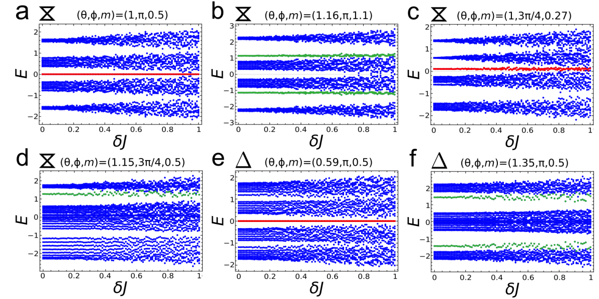
The second kind of non-protected topological states are those in the first and third gaps of the system. The protecting symmetries can only cause their energies to have opposite values, not to be fixed at a given value. For this reason, they are not prevented from drifting into the bulk bands when a high level of disorder is present.
In Fig. 10 (b), the response of non-protected states in the first and third gaps of the -CSSH ladder spectrum can be seen for different values of . As disorder increases, their energies start fluctuating around their value in the clean system. This also happens in the topological crystalline insulator case, Fig. 10 (d), and for the left edge modes in the -CSSH ladder which do not follow the usual bulk-boundary correspondence, Fig. 10 (f). In these two last cases, the fluctuations are more pronounced than in Fig. 10 (b), probably due to the absence of PH and chiral symmetries in (d), and the different nature of the states in (f). In all the analyzed models, except in the topological crystalline insulator phase, the spectrum is still symmetric around zero energy, because the PH and chiral symmetries are not broken. This means that when the state in the first gap drift upwards, the one in the third gap will drift downwards, and vice versa.
Appendix F Rhombus chain implementation
We consider a generalized rhombus chain Hamiltonian with a 6-site unit cell (see Fig. 8). We label the upper states and , the lower states are and , and the middle states are and :
| (66) |
where and . The phases implement a magnetic flux of through each rhombus of the chain, and can be generated using Floquet driving [27].
If we consider the regime where , the Hilbert space of the system will decouple into a low-energy subspace, with zero occupation in the middle sites, and a high-energy subspace. As indicated in [27], the low-energy subspace has the geometry of a Creutz ladder. Hence, changing the tunneling amplitudes in certain ways will let us obtain the different CSSH ladders. In particular, all topological flat band ladders and the SSH-like topological zero modes of the -CSSH ladder can be implemented in a straight-forward way. This can allow experimentalists to explore the various topological zero modes of Section 4 and Appendix C, and the flat-band dynamics of the models. The hopping amplitudes can be tuned by simply changing the distance between waveguides.
The low-energy effective Hamiltonian, obtained using a Schrieffer-Wolff transformation [115], is:
| (67) |
where and is the CSSH Hamiltonian of equation (1), with the following parameters:
In the most general case, the vertical amplitudes are not real.
The hourglass CSSH ladder can be obtained by choosing the parameters:
which generates the amplitudes:
with an additional on-site energy of on all sites. This model is represented in Fig. 8 (b), with long (short) links to represent weak (strong) tunneling amplitudes. If , and the flat-band -CSSH ladder is obtained. If , and the ladder has SSH-like topological zero modes if . For other values of , the vertical links have the same magnitude and opposite phase. They are always non-zero, so the rungless, non- flux topological case cannot be obtained in this way.
The rhomboid CSSH ladder Hamiltonian is obtained from (67) if we choose:
with the parameters:
This lattice is depicted in Fig. 8 (c). In the -flux case, , and we can choose to keep all on-site energies equal and obtain the topological flat-band -CSSH ladder. For other values of , might be chosen to get , and then the on-site energies could be compensated using the appropriate chemical potentials on the rhombus chain sites. Like in the hourglass case, the rungless non--flux case cannot be achieved in this way.
In this model, the energies cannot be made equal by fixing , so they must be compensated using on-site potentials. If , then and the topological flat-band case is obtained. Like in the other cases, the regime is not a strong topological phase, because is finite there. The -flux case with , which belongs to the D class, cannot be obtained directly using this method. To implement it, an additional tunneling amplitude of value could be established between the top and bottom sites of each rhombi, to create the vertical links of the ladder. This makes the lattice similar to the cold atom proposal in [12], and both of them could be used to implement the rungless topological regime for any value of , and also the -flux with case. In the -CSSH ladder, the latter corresponds to the D-class TI.
References
- Altland and Zirnbauer [1997] A. Altland and M. R. Zirnbauer, Nonstandard symmetry classes in mesoscopic normal-superconducting hybrid structures, Physical Review B 55, 1142 (1997).
- Lang and Büchler [2017] N. Lang and H. P. Büchler, Topological networks for quantum communication between distant qubits, npj Quantum Information 3, 47 (2017).
- Mei et al. [2018] F. Mei, G. Chen, L. Tian, S. L. Zhu, and S. Jia, Robust quantum state transfer via topological edge states in superconducting qubit chains, Physical Review A 98, 012331 (2018).
- Qi et al. [2020] L. Qi, G. L. Wang, S. Liu, S. Zhang, and H. F. Wang, Engineering the topological state transfer and topological beam splitter in an even-sized Su-Schrieffer-Heeger chain, Physical Review A 102, 022404 (2020).
- Estarellas et al. [2017] M. P. Estarellas, I. D’Amico, and T. P. Spiller, Topologically protected localised states in spin chains, Scientific Reports 7, 42904 (2017).
- Boross et al. [2019] P. Boross, J. K. Asbóth, G. Széchenyi, L. Oroszlány, and A. Pályi, Poor man’s topological quantum gate based on the Su-Schrieffer-Heeger model, Physical Review B 100, 045414 (2019).
- Tovmasyan et al. [2013] M. Tovmasyan, E. P. Van Nieuwenburg, and S. D. Huber, Geometry-induced pair condensation, Physical Review B 88, 220510(R) (2013).
- Li and Chen [2015a] L. Li and S. Chen, Characterization of topological phase transitions via topological properties of transition points, Physical Review B 92, 085118 (2015a).
- Padavić et al. [2018] K. Padavić, S. S. Hegde, W. DeGottardi, and S. Vishveshwara, Topological phases, edge modes, and the Hofstadter butterfly in coupled Su-Schrieffer-Heeger systems, Physical Review B 98, 024205 (2018).
- Velasco and Paredes [2019] C. G. Velasco and B. Paredes, Classification of topological ladder models (2019), arXiv:1907.11460 .
- Piga et al. [2017] A. Piga, M. Lewenstein, S.-J. Ran, J. Jünemann, A. Bermúdez, and M. Rizzi, Exploring Interacting Topological Insulators with Ultracold Atoms: The Synthetic Creutz-Hubbard Model, Physical Review X 7, 031057 (2017).
- Sun and Lim [2017] N. Sun and L.-K. K. Lim, Quantum charge pumps with topological phases in a Creutz ladder, Physical Review B 96, 035139 (2017).
- Kuno [2020] Y. Kuno, Extended flat band, entanglement, and topological properties in a Creutz ladder, Physical Review B 101, 184112 (2020).
- van Dalum et al. [2021] G. A. R. van Dalum, C. Ortix, and L. Fritz, Magnetic impurities along the edge of a quantum spin Hall insulator: Realizing a one-dimensional AIII insulator, Physical Review B 103, 075115 (2021).
- Liu and Hersam [2019] X. Liu and M. C. Hersam, 2D materials for quantum information science, Nature Reviews Materials 4, 669-684 (2019).
- Gholizadeh et al. [2018] S. Gholizadeh, M. Yahyavi, and B. Hetényi, Extended Creutz ladder with spin-orbit coupling: A one-dimensional analog of the Kane-Mele model, Epl 122, 27001 (2018).
- Creutz [1999] M. Creutz, End States, Ladder Compounds, and Domain-Wall Fermions, Physical Review Letters 83, 2636-2639 (1999).
- Vidal et al. [2000] J. Vidal, B. Douçot, R. Mosseri, and P. Butaud, Interaction induced delocalization for two particles in a periodic potential, Phys. Rev. Lett. 85, 3906 (2000).
- Douçot and Vidal [2002] B. Douçot and J. Vidal, Pairing of Cooper pairs in a fully frustrated Josephson-junction chain, Phys. Rev. Lett. 88, 227005 (2002).
- Creffield and Platero [2010] C. E. Creffield and G. Platero, Coherent control of interacting particles using dynamical and Aharonov-Bohm phases, Physical Review Letters 105, 086804 (2010).
- Pelegrí et al. [2019] G. Pelegrí, A. M. Marques, R. G. Dias, A. J. Daley, J. Mompart, and V. Ahufinger, Topological edge states and Aharanov-Bohm caging with ultracold atoms carrying orbital angular momentum, Phys. Rev. A 99, 023613 (2019).
- Vidal et al. [1998] J. Vidal, R. Mosseri, and B. Douçot, Aharonov-Bohm cages in two-dimensional structures, Phys. Rev. Lett. 81, 5888 (1998).
- Vidal et al. [2001] J. Vidal, P. Butaud, B. Douçot, and R. Mosseri, Disorder and interactions in Aharonov-Bohm cages, Phys. Rev. B 64, 155306 (2001).
- Abilio et al. [1999] C. C. Abilio, P. Butaud, T. Fournier, B. Pannetier, J. Vidal, S. Tedesco, and B. Dalzotto, Magnetic field induced localization in a two-dimensional superconducting wire network, Physical Review Letters 83, 5102-5105 (1999).
- Naud et al. [2001] C. Naud, G. Faini, and D. Mailly, Aharonov-Bohm cages in 2D normal metal networks, Physical Review Letters 86, 5104-5107 (2001).
- Shinohara et al. [2002] K. Shinohara, T. Aoki, and A. Morinaga, Scalar Aharonov-Bohm effect for ultracold atoms, Physical Review A 66, 042106 (2002).
- Mukherjee et al. [2018] S. Mukherjee, M. Di Liberto, P. Öhberg, R. R. Thomson, and N. Goldman, Experimental Observation of Aharonov-Bohm Cages in Photonic Lattices, Physical Review Letters 121, 075502 (2018).
- Kremer et al. [2020] M. Kremer, I. Petrides, E. Meyer, M. Heinrich, O. Zilberberg, and A. Szameit, A square-root topological insulator with non-quantized indices realized with photonic Aharonov-Bohm cages, Nature Communications 11, 907 (2020).
- Jörg et al. [2020] C. Jörg, G. Queraltó, M. Kremer, G. Pelegrí, J. Schulz, A. Szameit, G. von Freymann, J. Mompart, and V. Ahufinger, Artificial gauge field switching using orbital angular momentum modes in optical waveguides, Light: Science & Applications 9, 150 (2020).
- Cao et al. [2018] Y. Cao, V. Fatemi, S. Fang, K. Watanabe, T. Taniguchi, E. Kaxiras, and P. Jarillo-Herrero, Unconventional superconductivity in magic-angle graphene superlattices, Nature 556, 43-50 (2018).
- Takayoshi et al. [2013] S. Takayoshi, H. Katsura, N. Watanabe, and H. Aoki, Phase diagram and pair Tomonaga-Luttinger liquid in a Bose-Hubbard model with flat bands, Physical Review A 88, 063613 (2013).
- Mondaini et al. [2018] R. Mondaini, G. G. Batrouni, and B. Grémaud, Pairing and superconductivity in the flat band: Creutz lattice, Physical Review B 98, 155142 (2018).
- Zurita et al. [2019] J. Zurita, C. E. Creffield, and G. Platero, Topology and interactions in the photonic Creutz and Creutz-Hubbard ladders, Advanced Quantum Technologies 3, 1900105 (2019).
- Hügel and Paredes [2014] D. Hügel and B. Paredes, Chiral ladders and the edges of quantum Hall insulators, Physical Review A 89, 023619 (2014).
- Zhou and Du [2019] L. Zhou and Q. Du, Floquet topological phases with fourfold-degenerate edge modes in a driven spin-1/2 Creutz ladder, Physical Review A 101, 033607 (2019).
- Molignini [2020] P. Molignini, Edge mode manipulation through commensurate multifrequency driving, Physical Review B 102, 235143 (2020).
- Liu et al. [2019] Z. X. Liu, Z. H. Li, and A. M. Wang, Fractional charged edge states in ladder topological insulators, Journal of Physics Condensed Matter 31, 125402 (2019).
- Sticlet et al. [2014] D. Sticlet, L. Seabra, F. Pollmann, and J. Cayssol, From fractionally charged solitons to Majorana bound states in a one-dimensional interacting model, Physical Review B 89, 115430 (2014).
- Budich and Ardonne [2013] J. C. Budich and E. Ardonne, Equivalent topological invariants for one-dimensional Majorana wires in symmetry class , Phys. Rev. B 88, 075419 (2013).
- Lin et al. [2017] Y. Lin, W. Hao, M. Wang, J. Qian, and H. Guo, Topological superconductors from one-dimensional periodically modulated Majorana chains, Scientific Reports 7, 9210 (2017).
- Martinez Alvarez and Coutinho-Filho [2019] V. M. Martinez Alvarez and M. D. Coutinho-Filho, Edge states in trimer lattices, Phys. Rev. A 99, 013833 (2019).
- Asbóth et al. [2015] J. K. Asbóth, L. Oroszlány, and A. Pályi, A Short Course on Topological Insulators (Springer, 2015).
- Bello et al. [2016] M. Bello, C. E. Creffield, and G. Platero, Long-range doublon transfer in a dimer chain induced by topology and ac fields, Scientific Reports 6, 22562 (2016).
- Ivanov and Richter [1997] N. Ivanov and J. Richter, Competition between plaquette and dimer phases in Heisenberg chains, Physics Letters A 232, 308-312 (1997).
- Richter et al. [1998] J. Richter, N. B. Ivanov, and J. Schulenburg, The antiferromagnetic spin-1/2 chain with competing dimers and plaquettes: Numerical versus exact results, Journal of Physics Condensed Matter 10, 3635-3649 (1998).
- Čanová et al. [2004] L. Čanová, J. Strečka, and M. Jaščur, Exact results of the Ising-Heisenberg model on the diamond chain with spin-1/2, Czechoslovak Journal of Physics 54, 579-582 (2004).
- Paulinelli et al. [2013] H. G. Paulinelli, S. M. De Souza, and O. Rojas, Thermal entanglement in an orthogonal dimer-plaquette chain with alternating Ising-Heisenberg coupling, Journal of Physics Condensed Matter 25, 306003 (2013).
- Verkholyak and Strečka [2013] T. Verkholyak and J. Strečka, Exact solution for a quantum spin-12 Ising-Heisenberg orthogonal-dimer chain with Heisenberg intradimer and Ising interdimer interactions, Physical Review B 88, 134419 (2013).
- Leykam et al. [2018] D. Leykam, A. Andreanov, and S. Flach, Artificial flat band systems: From lattice models to experiments, Advances in Physics: X 3, 1473052 (2018).
- Nandy [2019] A. Nandy, Analytical study of quasi-one dimensional flat band networks and slow light analogue, Acta Physica Polonica A 136, 164-173 (2019).
- Rojas et al. [2019] O. Rojas, J. Strečka, M. L. Lyra, and S. M. De Souza, Universality and quasicritical exponents of one-dimensional models displaying a quasitransition at finite temperatures, Physical Review E 99, 042117 (2019).
- Gálisová et al. [2021] L. Gálisová, J. Strečka, T. Verkholyak, and S. Havadej, Magnetization plateaus and bipartite entanglement of an exactly solved spin-1/2 Ising-Heisenberg orthogonal-dimer chain, Physica E: Low-Dimensional Systems and Nanostructures 125, 114089 (2021).
- Yan and Wan [2014] Z. Yan and S. Wan, Topological phases, topological flat bands, and topological excitations in a one-dimensional dimerized lattice with spin-orbit coupling, EPL 107, 47007 (2014).
- Han et al. [2014] S. Han, H. Jiang, X. Li, and S. Xie, Spontaneous spin polarization in organic thiophene oligomers, Organic Electronics 15, 240-244 (2014).
- Jiang et al. [2015] H. Jiang, C. Zhang, X. Hu, G. Hu, and S. Xie, Spin polarization of polaron in quasi-one dimensional organic system, Modern Physics Letters B 29, 1450266 (2015).
- Bahari and Hosseini [2020] M. Bahari and M. V. Hosseini, Topological properties of a generalized spin–orbit-coupled Su–Schrieffer–Heeger model, Physica E: Low-Dimensional Systems and Nanostructures 119, 113973 (2020).
- Volkova and Marinin [2017] L. M. Volkova and D. V. Marinin, Frustrated Antiferromagnetic Spin Chains of Edge-Sharing Tetrahedra in Volcanic Minerals K3Cu3(Fe0.82Al0.18)O2(SO4)4 and K4Cu4O2(SO4)4MeCl, Journal of Superconductivity and Novel Magnetism 30, 959-971 (2017).
- Brenig and Becker [2001] W. Brenig and K. W. Becker, Magnetism of a tetrahedral cluster spin chain, Physical Review B 64, 214413 (2001).
- Ootomo and Ono [2000] F. Ootomo and Y. Ono, Acoustic polaron in a ladder-type electron-lattice system, Journal of the Physical Society of Japan 69, 3320-3327 (2000).
- Zhang and Zhou [2017] S. L. Zhang and Q. Zhou, Two-leg Su-Schrieffer-Heeger chain with glide reflection symmetry, Physical Review A 95, 061601 (2017).
- Nersesyan [2020] A. A. Nersesyan, Phase diagram of an interacting staggered Su-Schrieffer-Heeger two-chain ladder close to a quantum critical point, Physical Review B 102, 045108 (2020).
- Jangjan and Hosseini [2020] M. Jangjan and M. V. Hosseini, Floquet engineering of topological metal states and hybridization of edge states with bulk states in dimerized two-leg ladders, Scientific Reports 10, 14256 (2020).
- Ryu et al. [2020] J.-W. Ryu, S. Woo, N. Myoung, and H. C. Park, Topological edge states in bowtie ladders with different cutting edges (2020), arXiv:2012.00270 .
- Drescher and Mielke [2017] M. Drescher and A. Mielke, Hard-core bosons in flat band systems above the critical density, European Physical Journal B 90, 217 (2017).
- Schnyder et al. [2008] A. P. Schnyder, S. Ryu, A. Furusaki, and A. W. W. Ludwig, Classification of topological insulators and superconductors in three spatial dimensions, Phys. Rev. B 78, 195125 (2008).
- Kitaev [2009] A. Kitaev, Periodic table for topological insulators and superconductors, AIP Conference Proceedings 1134, 22-30 (2009).
- Stanescu [2016] T. D. Stanescu, Introduction to Topological Quantum Matter and Quantum Computation (CRC Press, 2016).
- Alaeian et al. [2019] H. Alaeian, C. W. S. Chang, M. V. Moghaddam, C. M. Wilson, E. Solano, and E. Rico, Creating lattice gauge potentials in circuit QED: The bosonic Creutz ladder, Physical Review A 99, 053834 (2019).
- Leonforte et al. [2021] L. Leonforte, A. Carollo, and F. Ciccarello, Vacancy-like Dressed States in Topological Waveguide QED, Phys. Rev. Lett. 126, 063601 (2021).
- Jackiw [2012] R. Jackiw, Fractional and Majorana fermions: the physics of zero-energy modes, Physica Scripta T146, 014005 (2012).
- Herviou [2017] M. L. Herviou, Topological Phases and Majorana Fermions, Ph.D. thesis, Université Paris-Saclay (2017).
- Pérez-González et al. [2019a] B. Pérez-González, M. Bello, Á. Gómez-León, and G. Platero, Interplay between long-range hopping and disorder in topological systems, Physical Review B 99, 035146 (2019a).
- Su et al. [1979] W. P. Su, J. R. Schrieffer, and A. J. Heeger, Solitons in Polyacetylene, Phys. Rev. Lett. 42, 1698 (1979).
- Zak [1989] J. Zak, Berry’s phase for energy bands in solids, Phys. Rev. Lett. 62, 2747 (1989).
- Ryu and Hatsugai [2002] S. Ryu and Y. Hatsugai, Topological Origin of Zero-Energy Edge States in Particle-Hole Symmetric Systems, Physical Review Letters 89, 077002 (2002).
- Lau and Ortix [2018] A. Lau and C. Ortix, Novel topological insulators from crystalline symmetries, European Physical Journal: Special Topics 227, 1309 (2018).
- Cariglia [2014] M. Cariglia, Hidden symmetries of dynamics in classical and quantum physics, Reviews of Modern Physics 86, 1283-1336 (2014).
- Hou [2013] J. M. Hou, Hidden-Symmetry-Protected Topological Semimetals on a Square Lattice, Physical Review Letters 111, 130403 (2013).
- Fukui et al. [2013] T. Fukui, K. I. Imura, and Y. Hatsugai, Symmetry protected weak topological phases in a superlattice, Journal of the Physical Society of Japan 82, 073708 (2013).
- Li and Chen [2015b] L. Li and S. Chen, Hidden-symmetry-protected topological phases on a one-dimensional lattice, EPL 109, 40006 (2015b).
- Hou and Chen [2016] J. M. Hou and W. Chen, Hidden-symmetry-protected quantum pseudo-spin Hall effect in optical lattices, Physical Review A 93, 063626 (2016).
- Hou and Chen [2017] J. M. Hou and W. Chen, Hidden symmetry-protected Z2 topological insulator in a cubic lattice, Physical Review B 96, 235108 (2017).
- Xiao and An [2018] J. Xiao and J. An, Boundary states in the chiral symmetric systems with a spatial symmetry, Journal of Physics Condensed Matter 30, 055002 (2018).
- Marques and Dias [2019] A. M. Marques and R. G. Dias, One-dimensional topological insulators with noncentered inversion symmetry axis, Physical Review B 100, 041104 (2019).
- Wang et al. [2018] L. Wang, W. Cai, M. Bie, X. Zhang, and J. Xu, Zak phase and topological plasmonic Tamm states in one-dimensional plasmonic crystals, Optics Express 26, 28963 (2018).
- Wang et al. [2019] H.-X. Wang, G.-Y. Guo, and J.-H. Jiang, Band topology in classical waves: Wilson-loop approach to topological numbers and fragile topology, New Journal of Physics 21, 093029 (2019).
- Zhu et al. [2018] W. Zhu, Y.-q. Ding, J. Ren, Y. Sun, Y. Li, H. Jiang, and H. Chen, Zak phase and band inversion in dimerized one-dimensional locally resonant metamaterials, Phys. Rev. B 97, 195307 (2018).
- Deng et al. [2013] S. Deng, G. Ortiz, and L. Viola, Multiband -wave topological superconductors: Role of dimensionality and magnetic field response, Phys. Rev. B 87, 205414 (2013).
- Li et al. [2016] L. Li, C. Yang, and S. Chen, Topological invariants for phase transition points of one-dimensional Z2 topological systems, European Physical Journal B 89, 195 (2016).
- Ke et al. [2016] Y. Ke, X. Qin, F. Mei, H. Zhong, Y. S. Kivshar, and C. Lee, Topological phase transitions and Thouless pumping of light in photonic waveguide arrays, Laser & Photonics Reviews 10, 995 (2016).
- Ganeshan et al. [2013] S. Ganeshan, K. Sun, and S. Das Sarma, Topological zero-energy modes in gapless commensurate Aubry-André- Harper models, Physical Review Letters 110, 180403 (2013).
- Kang et al. [2018] J. H. Kang, J. H. Han, and Y. Shin, Realization of a Cross-Linked Chiral Ladder with Neutral Fermions in a 1D Optical Lattice by Orbital-Momentum Coupling, Physical Review Letters 121, 150403 (2018).
- Hyoun Kang et al. [2020] J. Hyoun Kang, J. Ho Han, and Y. Shin, Creutz ladder in a resonantly shaken 1D optical lattice, New Journal of Physics 22, 013023 (2020).
- Hung et al. [2021] J. S. C. Hung, J. H. Busnaina, C. W. S. Chang, A. M. Vadiraj, I. Nsanzineza, E. Solano, H. Alaeian, E. Rico, and C. M. Wilson, Quantum Simulation of the Bosonic Creutz Ladder with a Parametric Cavity, Phys. Rev. Lett. 127, 100503 (2021).
- Han et al. [2020] J. Han, A. A. Sukhorukov, and D. Leykam, Disorder-protected quantum state transmission through helical coupled-resonator waveguides, Photonics Research 8, 10, B15-B24 (2020).
- Barbarino et al. [2019] S. Barbarino, D. Rossini, M. Rizzi, R. Fazio, G. E. Santoro, and M. Dalmonte, Topological Devil’s staircase in atomic two-leg ladders, New Journal of Physics 21, 043048 (2019).
- Resta [1998] R. Resta, Quantum-Mechanical Position Operator in Extended Systems, Physical Review Letters 80, 1800 (1998).
- Vanderbilt [2018] D. Vanderbilt, Berry phase in electronic structure theory (Cambridge University Press, 2018).
- Bena and Montambaux [2009] C. Bena and G. Montambaux, Remarks on the tight-binding model of graphene, New Journal of Physics 11, 095003 (2009).
- Cayssol and Fuchs [2021] J. Cayssol and J. N. Fuchs, Topological and geometrical aspects of band theory, Journal of Physics: Materials 4, 034007 (2021).
- Fuchs and Piéchon [2021] J. N. Fuchs and F. Piéchon, Electric polarization of one-dimensional inversion-symmetric two-band insulators (2021), arXiv:2106.03595 .
- Delplace et al. [2011] P. Delplace, D. Ullmo, and G. Montambaux, Zak phase and the existence of edge states in graphene, Physical Review B 84, 195452 (2011).
- Longhi [2018] S. Longhi, Probing one-dimensional topological phases in waveguide lattices with broken chiral symmetry, Optics Letters 43, 4639 (2018).
- Bello et al. [2019] M. Bello, G. Platero, J. I. Cirac, and A. González-Tudela, Unconventional quantum optics in topological waveguide QED, Science Advances 5, eaaw0297 (2019).
- Aihara et al. [2020] Y. Aihara, M. Hirayama, and S. Murakami, Anomalous dielectric response in insulators with the Zak phase, Phys. Rev. Research 2, 033224 (2020).
- Pérez-González et al. [2019b] B. Pérez-González, M. Bello, G. Platero, and Á. Gómez-León, Simulation of 1D Topological Phases in Driven Quantum Dot Arrays, Physical Review Letters 123, 126401 (2019b).
- Jiao et al. [2021] Z.-Q. Jiao, S. Longhi, X.-W. Wang, J. Gao, W.-H. Zhou, Y. Wang, Y.-X. Fu, L. Wang, R.-J. Ren, L.-F. Qiao, and X.-M. Jin, Experimentally Detecting Quantized Zak Phases without Chiral Symmetry in Photonic Lattices, Physical Review Letters 127, 147401 (2021).
- Cooper et al. [2019] N. R. Cooper, J. Dalibard, and I. B. Spielman, Topological bands for ultracold atoms, Reviews of Modern Physics 91, 015005 (2019).
- Atala et al. [2013] M. Atala, M. Aidelsburger, J. Barreiro, D. Abanin, T. Kitagawa, E. Demler, and I. Bloch, Direct measurement of the Zak phase in topological Bloch bands, Nature Physics , 795 (2013).
- Marzari and Vanderbilt [1997] N. Marzari and D. Vanderbilt, Maximally localized generalized Wannier functions for composite energy bands, Physical Review B 56, 12847 (1997).
- Creffield [2020] C. E. Creffield, Controlling spin without magnetic fields: The Bloch-Rashba rotator, Phys. Rev. B 102, 085436 (2020).
- Jafari et al. [2019] R. Jafari, H. Johannesson, A. Langari, and M. A. Martin-Delgado, Quench dynamics and zero-energy modes: the case of the Creutz model, Physical Review B 99, 054302 (2019).
- Tovmasyan et al. [2018] M. Tovmasyan, S. Peotta, L. Liang, P. Törmä, and S. D. Huber, Preformed pairs in flat Bloch bands, Phys. Rev. B 98, 134513 (2018).
- Nelson et al. [2021] A. Nelson, T. Neupert, T. c. v. Bzdušek, and A. Alexandradinata, Multicellularity of Delicate Topological Insulators, Phys. Rev. Lett. 126, 216404 (2021).
- Hofmann and Potthoff [2012] F. Hofmann and M. Potthoff, Doublon dynamics in the extended Fermi-Hubbard model, Physical Review B 85, 205127 (2012).
- Raoux et al. [2014] A. Raoux, M. Morigi, J.-N. Fuchs, F. Piéchon, and G. Montambaux, From Dia- to Paramagnetic Orbital Susceptibility of Massless Fermions, Phys. Rev. Lett. 112, 026402 (2014).
- Illes and Nicol [2016] E. Illes and E. J. Nicol, Magnetic properties of the model: Magneto-optical conductivity and the Hofstadter butterfly, Physical Review B 94, 125435 (2016).
- Illes and Nicol [2017] E. Illes and E. J. Nicol, Klein tunneling in the model, Physical Review B 95, 235432 (2017).
