Predictive control barrier functions: Enhanced safety mechanisms for learning-based control

Abstract

While learning-based control techniques often outperform classical controller designs, safety requirements limit the acceptance of such methods in many applications. Recent developments address this issue through so-called predictive safety filters, which assess if a proposed learning-based control input can lead to constraint violations and modifies it if necessary to ensure safety for all future time steps. The theoretical guarantees of such predictive safety filters rely on the model assumptions and minor deviations can lead to failure of the filter putting the system at risk. This paper introduces an auxiliary soft-constrained predictive control problem that is always feasible at each time step and asymptotically stabilizes the feasible set of the original predictive safety filter problem, thereby providing a recovery mechanism in safety-critical situations. This is achieved by a simple constraint tightening in combination with a terminal control barrier function. By extending discrete-time control barrier function theory, we establish that the proposed auxiliary problem provides a ‘predictive’ control barrier function. The resulting algorithm is demonstrated using numerical examples.

Constrained control, NL predictive control, Intelligent systems, Safety

Appendix A INTRODUCTION

The increasing availability of computational resources opens new perspectives for control engineering, and in particular enables learning-based control, which has shown the potential of solving complex high-level tasks. Demonstrations include, e.g., human-machine interactions, where solely a ‘black-box’ reward signal describes the desired system behavior. As such a general problem formulation is not addressed by classical controller specifications in terms of stability w.r.t. pre-specified setpoints or reference trajectories, there is a renewed interest in the development of universal mechanisms to ensure safety of the resulting closed-loop system.

Using a modular approach to control system safety and performance as proposed in [1], various methods have recently been developed, such as, e.g., control barrier functions [2] and reachability analysis based safety frameworks [3] to ensure safety in the form of constraint satisfaction, independent of a specific control task. These methods typically consist of a safety controller that renders a safe subset of the system constraints invariant. These two components allow to enhance an arbitrary performance controller with safety guarantees as follows: As long as the system state evolution under the performance controller is contained in the safe invariant set, the safety mechanism passively monitors proposed control signals. However, as soon as the system state would leave the safe set, the safety mechanism actively overrules the performance controller and leverages the safety controller to render the safe set invariant. As the computation of the required safe set and safety controller is very difficult in general, the resulting control performance is often limited due to conservative approximations or the required design computations are restricted to small-scale systems up to 3-4 state dimensions due to the curse of dimensionality.

To overcome this limitation, recent concepts extend potentially conservative safe sets and safety controllers during closed-loop operation by a just-in-time computation of safe backup plans from the current system state, which are required to terminate in a potentially conservative safe set. These methods are also known as active set reachability [4], SHERPA [5], model predictive safety certification (MPSC) [6], predictive safety filters (PSF) [7], and predictive shielding [8]. While some of them are based on MPC techniques [9, 6, 7, 8], other approaches, e.g. [4], extend a conservative safe set online through an explicit safety controller. As shown in [10], these approaches can significantly reduce conservativeness and thereby increase acceptance of such safety mechanisms.

Despite promising theoretical and experimental results, the major drawback of such just-in-time safety computations are unexpected external disturbances or constraint violating initial conditions, which cannot always be anticipated at the controller design stage. In such cases, even for minor errors in design assumptions, the corresponding online problem can become infeasible, failing to provide a safe input, when it would be most crucial to recover the system from constraint violations.

A.1 Contributions

This paper proposes a predictive barrier function approach to recover infeasible predictive controllers in an asymptotically stable fashion through a soft constraint recovery mechanism. In particular, we consider recovery of predictive safety filter problems [9, 6, 7], which are commonly used in combination with learning-based control techniques to ensure safety and which are lacking intrinsic stability properties compared to, e.g., classical MPC [11]. Different from a simple softening of the state constraints ‘out-of-the-box’ [12], we propose a softened predictive safety filter problem, denoted predictive barrier function problem, which renders the feasible set of the predictive safety filter Lyapunov stable, thereby enabling a reliable recovery of the safety guarantees from unexpected disturbances or unsafe initial conditions.

The primary mechanism of the predictive barrier function is to employ a control barrier function on the last predicted state with a corresponding terminal safe set. Through a generalization of existing discrete-time control barrier function theory, we formally establish that the value function of the predictive barrier function problem itself qualifies as a control barrier function, thereby enlarging the region of attraction of a potentially conservative terminal control barrier function. As a result, we obtain Lyapunov stability properties with respect to the feasible safe set of the original predictive safety filter problem.

The novel relation between predictive safety filters and control barrier functions additionally allows for combining recent results from control barrier function literature, such as safe reinforcement learning with convergence guarantees [13], together with significantly less restrictive predictive safety filters. Furthermore, since the optimal value function of the predictive barrier function problem represents a continuous measure of safety, it can efficiently be approximated using, e.g., artificial neural networks. This allows for a practical implementation for highly nonlinear dynamical systems, where the corresponding online problem to evaluate the predictive barrier function is challenging to solve in real-time.

We provide a design procedure to synthesize the proposed method and demonstrate the ability to recover infeasible predictive safety filters using numerical simulations, i.e., a basic linear 2D example and a nonlinear vehicle example.

A.2 Related work

While online predictive safety mechanisms that assume a perfect system knowledge [4, 10] can quickly become infeasible, robust and stochastic formulations [5, 9, 6, 7, 8] provide safety through recursive feasibility of the problem despite external disturbances. Nevertheless, the underlying assumption of these techniques is a feasible initial condition as well as an accurate uncertainty description of the disturbance, which can be difficult to ensure and can cause controller failure if not satisfied. We overcome this limitation by proposing a concept for state constraint relaxation that provides a feasible problem to compute stabilizing inputs, even for cases, in which robust or stochastic formulations would become infeasible.

Infeasibility issues of online predictive control problems have also been investigated in the model predictive control (MPC) literature, e.g. [12, 14], the results are, however, limited to linear systems with polytopic state constraints. Furthermore, stability properties of the closed-loop system are typically given with respect to a steady-state rather than the original feasible set of the hard constrained model predictive control problem, which can lead to a longer duration of constraint violation in closed-loop in favor of stability with respect to the origin. Related to these techniques, the notion of input-to-state stability in MPC [15] can provide similar recovery properties from disturbances or infeasible initial conditions, which are, however, also generally coupled to a stability analysis with respect to the origin and rely on a positive definite cost function in the MPC problem together with additional assumptions in the nonlinear case.

An alternative MPC-related technique to provide feasibility of online MPC problems is based on so-called any-time MPC algorithms [16, 17] that use a relaxation at the optimization algorithm level, to ensure similar stability properties as presented in [14]. This approach is also tied to a positive definite stage cost function, linear dynamics and polytopic constraints, as well as a particular optimization approach for solving the MPC problem. By ensuring feasibility through a modified formulation of the predictive control problem, the presented approach allows for leveraging recent developments in the active field of fast real-time optimization techniques [18, 19] without relying on a specific optimization algorithm.

Combining MPC control design with control Lyapunov or control barrier functions has also been proposed in [20, 21, 22], where the idea is to impose an explicit barrier function constraint on each predicted system state, which provides guarantees in terms of constraint satisfaction. While there also exists a soft-constrained formulation using control Lyapunov functions [23], the main limitation of these approaches is that each predicted state must be contained in the domain of the control barrier/control Lyapunov function. As the design of these functions is a challenging task for general systems, their region of attraction is often restricted to small subsets around linearization points and can significantly limit the set of states for which the resulting MPC provides theoretical guarantees. In contrast, we impose softened state constraints along the planning horizon and only combine the last predicted state with a control barrier function, which allows for a simple design procedure with an increased feasible set.

A.3 Notation and common definitions

The distance between a vector $x\in\mathbb{R}^{n}$ and a set $\mathcal{A}\subseteq\mathbb{R}^{n}$ is defined as $|x|_{\mathcal{A}}\coloneqq\inf_{y\in\mathcal{A}}||x-y||$. By $\mathbbm{1}_{n}$ we denote the vector of ones with length $n\in\mathbb{N}^{+}$ and $\max(x,y)$ with $x,y\in\mathbb{R}^{n}$ equals the element-wise maximum value. The set of symmetric positive definite matrices of size $n\times n$ is denoted by $S^{n}_{++}$.

Definition A.1.

A set $\mathcal{A}\subseteq\mathbb{R}$ is said to be positively invariant for the autonomous system $x(k+1)=g(x(k))$ if for every $x(0)\in\mathcal{A}$ it holds for all $k\in\mathbb{N}$ that $x(k)\in\mathcal{A}$.

Appendix B Preliminaries

Figure 1: The concept of a model predictive safety filter: Using the current state $x(k)$, a task-specific performance controller provides an input $u_{p}(x(k))$, which is processed by the predictive safety filter (5) and then applied to the real system (1).

Figure 2: Inner workings of the predictive safety filter (5): Based on the current state $x(k)$, the predicted state sequence terminates in the terminal safe set $\SS_{f}$ (green set) after 5 planning steps. The feasible set of the safety filter problem $\mathbb{X}^{\mathrm{PSF}}$ (6), i.e. the set of states from which $\SS_{f}$ can be reached within $5$ time steps, is illustrated in blue and is a subset of the state constraint set $\mathbb{X}$ (black lines). For system states $x(\bar{k}_{1})$ and $x(\bar{k}_{2})$ outside the feasible set $\mathbb{X}^{\mathrm{PSF}}$, the safety filter cannot provide a safe input. We address this limitation in this work by introducing a softened reformulation that stabilizes the feasible set $\mathbb{X}^{\mathrm{PSF}}$ with enlarged region of attraction $\mathcal{D}_{\mathrm{PB}}$ in Section C.

We consider discrete-time control systems of the form

$$x(k+1)=f(x(k),u(k)),~{}k\in\mathbb{N},$$ (1)

with continuous dynamics $f:\mathbb{R}^{n}\times\mathbb{R}^{m}\rightarrow\mathbb{R}^{n}$ and initial condition $x(0)=x_{0}$ with $x_{0}\in\mathbb{R}^{n}$. The system is subject to hard physical input constraints of the form

$$u(k)\in\mathbb{U}\subset\mathbb{R}^{m},$$ (2)

with compact $\mathbb{U}$, and is required to satisfy safety constraints in the form of state constraints given by

$$x(k)\in\mathbb{X}\coloneqq\{x\in\mathbb{R}^{n}:c(x)\leq 0\}\subset\mathbb{R}^{n},$$ (3)

for all time steps $k\in\mathbb{N}$ where $c:\mathbb{R}^{n}\rightarrow\mathbb{R}^{n_{x}}$ is a continuous function. While the input constraints (2) can be generic compact subsets of $\mathbb{R}^{m}$, the state constraints (3) need to be represented as a set of nonlinear inequalities, which include, e.g., box, ellipsoidal, or polytopic constraints as relevant special cases. Relevant learning-based control applications or complex tasks via RL, for which a sufficiently accurate model (1) is available include inverse optimal control, imitation learning, or interactions with humans [24, Section 4]. In the following, we briefly review the predictive safety filter formulation as shown in Figure 1 and introduce a soft-constrained extension.

B.1 Predictive Safety Filter

The overall goal is to provide a modular approach to safety of task-specific performance controllers

$$u_{p}:\mathbb{R}^{n}\rightarrow\mathbb{R}^{m}$$ (4)

as originally proposed in [1], see Figure 1. Potentially unsafe inputs $u_{p}(x(k))$ are processed in real-time by a safety filter that decides based on the current system state if the input is safe to apply or if it needs to be modified. To implement the desired safety filter, we make use of an MPC-based concept called predictive safety filter as introduced in [9]. In particular, our goal is to extend the MPC-based mechanism from [9] to not only keep the system safe but to also recover the safety filter from constraint violations, which can result from unexpected external disturbances or infeasible initial conditions. To this end, we first recap the nominal formulation of a predictive safety filter as introduced in [24, Section 5] in the following, which we will then equip with a recovery mechanism in Section C.

A basic model predictive safety filter, realizing the safety filter block in Figure 1, is given by

$$\min_{u_{i|k}}~{}~{} \lVert{u_{p}(x(k))-u_{0|k}}\rVert$$ (5a)

s.t. $$\text{for all }i=0,..,N-1:$$

$$x_{0|k}=x(k),$$ (5b)

$$x_{i+1|k}=f(x_{i|k},u_{i|k}),$$ (5c)

$$u_{i|k}\in\mathbb{U},$$ (5d)

$$x_{i|k}\in\mathbb{X},$$ (5e)

$$x_{N|k}\in\SS_{f},$$ (5f)

where the resulting input applied to the system is given by $u(k)=u^{*}_{0|k}$. We use the subscript $i|k$ to emphasize predictive quantities, where, e.g., $x_{i|k}$ is the $i$-step-ahead prediction of the state, initialized at $x_{0|k}=x$ at time step $k$. Optimal states and inputs will be denoted by an asterisk, e.g. $u^{*}_{i|k}$ or $x^{*}_{i|k}$. The objective (5a) is to achieve minimal deviation between the first element of the predicted input sequence, $u^{*}_{0|k}$, and the currently requested performance input, $u_{p}(x(k))$, while satisfying state (5e) and input constraints (5d) for predicted time steps. By solving (5) at every time step, we obtain the desired filtering property as follows. If for a specific state $x(k)$ and proposed performance input $u_{p}(x(k))$ the objective (5a) is zero subject to all relevant system constraints for all future time steps, then the performance controller is safe and will directly be applied since $u^{*}_{0|k}=u_{p}(x(k))$. However, if the objective is greater than zero, the performance control input $u_{p}(x(k))$ at the current time step cannot be verified as safe and the safety filter mechanism overwrites the performance controller, i.e. $u^{*}_{0|k}\neq u_{p}(x(k))$. The PSF problem makes use of a terminal constraint on the last predicted state (5f), see Figure 2 (green set), which is typically assumed to be positive invariant for system (1) (Definition A.1) under a local safety control law satisfying state and input constraints. This technique from MPC literature ensures that initial feasibility of (5) at state $x(k)$ with corresponding optimal input sequence $u^{*}_{i|k}$ implies feasibility of (5) for future time steps in a recursive fashion. This can be shown easily through constructing a feasible candidate solution for time step $k+1$, which is given by $\bar{u}_{i|k+1}=\{u^{*}_{1|k},u^{*}_{2|k},..,u^{*}_{N|k},\tilde{u}_{f}\}$, where $\tilde{u}_{f}$ is selected such that $\bar{x}_{N|k+1}=f(x^{*}_{N|k},\tilde{u}_{f})\in\SS_{f}$ holds, which is possible due to the invariance property of $\SS_{f}$ [11, 25].

Recursive feasibility of (5) directly implies constraint satisfaction for all future time steps together with the fact that the feasible set

$$\mathbb{X}^{\mathrm{PSF}}\coloneqq\{x\in\mathbb{R}^{n}~{}|~{}\eqref{eq:opt_PSF}\text{ is feasible}\},$$ (6)

as illustrated in Figure 2 (blue set), is rendered forward invariant under $u(k)=u^{*}_{0|k}$ and realizes an implicitly defined safe set.

While there exist extensions of (5) that can deal with external disturbances in a robust [7] or stochastic manner [6], these methods rely on specific assumptions on the disturbance in the form of a known magnitude or probability distribution. These techniques therefore still suffer from infeasibility issues in case of unmodeled external disturbances $d(k)\in\mathbb{R}^{n}$ such that $f(x(k),u(k))+d(k)\notin\mathbb{X}^{\mathrm{PSF}}$ or even $f(x(k),u(k))+d(k)\notin\mathbb{X}$. These situations commonly arise in practice with severe consequences, as no sensible input can be generated from an infeasible PSF problem (5) to ensure system safety, as illustrated with states $x(\bar{k}_{1})$ and $x(\bar{k}_{2})$ in Figure 2. The goal in the following is to render the feasible set of the safety filter (6) in such situations asymptotically stable through a soft-constrained recovery mechanism.

B.2 Simplistic soft constrained predictive safety filter

Figure 3: Predictive safety filter with a simplistic soft constrained recovery mechanism: Based on the current state $x(k)$, the performance controller (4) provides a desired control input $u_{p}(x(k))$. At the same time, slack values $\xi_{i|k}^{*}$ are computed by either solving the simple feasibility problem (8) according to Section B.1 or by evaluating the predictive barrier function (9) as described in Section C, both ensuring existence of a feasible solution to the softened predictive safety filter problem (7) for all $x(k)\in\mathbb{R}^{n}$.

In practical implementations of the predictive safety filter, a softening of the state constraints as proposed, e.g., in [26, 12] for MPC, can guarantee feasibility of the online optimization problem (5) despite unexpected disturbances. In this section, we first recap a simplistic ‘separation of objectives’ approach and discuss its limitations, which motivates the predictive control barrier function presented in Section C. The simplistic soft constrained PSF problem is given by

$$\min_{u_{i|k}}~{}~{} \lVert{u_{p}(x(k))-u_{0|k}}\rVert$$ (7a)

s.t. $$\text{for all }i=0,..,N-1:$$

$$\eqref{eq:opt_PSF_init}-\eqref{eq:opt_PSF_input_cons},$$ (7b)

$$x_{i|k}\in\mathbb{X}(\xi_{i}^{*}),$$ (7c)

$$x_{N|k}\in\SS_{f}(\xi_{N}^{*}).$$ (7d)

Thereby, (7c), (7d) are soft constraints of the form $\mathbb{X}(\xi_{i|k}^{*})=\{x\in\mathbb{R}^{n}|c(x)\leq\xi_{i|k}^{*}\}$ with pre-computed slacks according to

$$\xi_{i|k}^{*}=\operatorname*{argmin}_{\xi_{i|k},u_{i|k}}~{}~{} ~{}\sum_{i=0}^{N}\|\xi_{i}\|$$ (8a)

s.t. $$\text{for all }i=0,..,N-1:$$ (8b)

$$\eqref{eq:opt_PSF_init}-\eqref{eq:opt_PSF_input_cons}$$ (8c)

$$x_{i|k}\in\mathbb{X}(\xi_{i}),~{}~{}0\leq\xi_{i},$$ (8d)

$$x_{N|k}\in\SS_{f}(\xi_{N}),~{}~{}0\leq\xi_{N},$$ (8e)

as depicted in Figure 3. This ensures feasibility of (7) for any input sequence, even if $x_{i|k}\notin\mathbb{X}$, in which case the violation is penalized in the objective for determining the slack values (8a). By construction, this two-step approach provides the same optimal solution as (5) for all $x\in\mathbb{X}^{\mathrm{PSF}}$ and preserves feasibility otherwise.

Remark B.1.

Although the additional feasibility problem (8) introduces a second optimization stage at each sampling time, it is important to note that it can be solved in parallel with the performance controller as it only depends on the current system state. Additionally, (8) provides a feasible warm start of (7), that can be leveraged by many optimization algorithms.

While (7) and (8) ensure feasibility, it is unclear if the resulting control input drives the state $x(k)$ back into $\mathbb{X}^{\mathrm{PSF}}$ at some future point in time from $x(0)\notin\mathbb{X}^{\mathrm{PSF}}$. In the following, we address this issue by introducing a modified formulation of the feasibility problem (8), called predictive barrier function problem, that ensures feasibility of the soft constrained predictive safety filter problem (7) and is guaranteed to recover feasibility of (5).

Appendix C Predictive control barrier functions

The proposed predictive control barrier function problem reads

$$h_{\mathrm{PB}}(x)\coloneqq\min_{u_{i|k},\xi_{i|k}}~{}~{} \alpha_{f}\xi_{N|k}+\sum_{i=0}^{N-1}\lVert{\xi_{i|k}}\rVert$$ (9a)

s.t. $$\text{for all }i=0,..,N-1:$$

$$x_{0|k}=x,$$ (9b)

$$x_{i+1|k}=f(x_{i|k},u_{i|k}),$$ (9c)

$$x_{i|k}\in\mathbb{X}_{i}(\xi_{i|k}),~{}0\leq\xi_{i|k},$$ (9d)

$$u_{i|k}\in\mathbb{U},$$ (9e)

$$h_{f}(x_{N|k})\leq\xi_{N|k},~{}0\leq\xi_{N|k},$$ (9f)

which implements a modified (tightened) state constraint (9d) as detailed in Section C.1 and a more specific terminal constraint (9f) as formalized in Section C.2 compared to (8). Problem (9) thereby provides a Lyapunov-like value function $h_{\mathrm{PB}}(x)\geq 0$, which ensures asymptotic stability of the set of states

$$\SS_{\mathrm{PB}}=\{x\in\mathbb{R}^{n}:h_{\mathrm{PB}}(x)=0\},$$ (10)

for which we can find an optimal solution to (9) without state constraint violations along the prediction. To this end, we guarantee a decrease of $h_{\mathrm{PB}}(x)$ for all $x\notin\SS_{\mathrm{PB}}$ between two consecutive time-steps under application of $u(k)=u^{*}_{0|k}$.

The decrease is achieved via two components. An iterative tightening of the state constraints along predictions in (9d), which is detailed in Section C.1, ensures a reduction of the slacks $\sum_{i=0}^{N-1}\lVert{\xi^{*}_{i|k}}\rVert$ from one time step to the next if $\xi^{*}_{i|k}\neq 0$ for some $i=1,..,N-1$. A decrease of the term $\alpha_{f}\xi^{*}_{N|k}$ in (9a) is obtained by introducing a terminal set of the form $\SS_{f}\coloneqq\{x\in\mathbb{R}^{n}|h_{f}(x)\leq 0\}$ and requiring $\SS_{f}$ to be a safe set corresponding to a so-called control barrier function $h_{f}(x)$ as it will be introduced in Section C.2.

These modifications will allow us in Section C.3 to establish that the proposed scheme as summarized in Algorithm 1 renders $\SS_{\mathrm{PB}}$ in (10) asymptotically stable. Note that due to the constraint tightening in (9d), the set $\SS_{\mathrm{PB}}$ is a subset of the nominal feasible set of the PSF problem (6), i.e. $\SS_{\mathrm{PB}}\subset\mathbb{X}^{\mathrm{PSF}}$. Establishing asymptotic stability of $\SS_{\mathrm{PB}}$ therefore implies the desired recovery from constraint violations.

Algorithm 1 Predictive safety filter with recovery mechanism

1:  for $k=0,1,2..$ do

2:     Measure system state $x(k)$

3:     Evaluate desired performance input $u_{p}(k)$ and determine slack values $\{\xi^{*}_{i|k}\}$ by solving (9) in parallel

4:     Solve

$$\{u^{*}_{i|k}\}\in\operatorname*{argmin}_{u_{i|k}}~{}~{} \lVert{u_{p}(x(k))-u_{0|k}}\rVert$$

s.t. $$\text{for all }i=0,..,N-1:$$

$$\eqref{eq:opt_PSF_init}-\eqref{eq:opt_PSF_input_cons},$$

$$x_{i|k}\in\mathbb{X}_{i}(\xi^{*}_{i|k}),$$

$$h_{f}(x_{N|k})\leq\xi^{*}_{N|k}.$$

5:     Apply $u(k)\leftarrow u^{*}_{0|k}$ to system (1)

6:  end for

C.1 Tightened soft constraints

While the simple state and terminal constraint softening from Section B.2 ensures feasibility, e.g., if $\xi^{*}_{0|k}=0$, $\xi^{*}_{j|k}\neq 0$, and $\xi^{*}_{N|k}=0$ for some $j>0$, it is not clear, whether the total amount of slack $\sum_{i=0}^{N}\|\xi_{i|k}^{*}\|$ will be reduced at the next time step $k+1$ using the scheme as depicted in Figure 3. More precisely, the construction of a feasible candidate at time $k+1$ using a common shifting operation of the optimal solution at time $k$ would only keep the amount of total slack constant.  This is due to the fact that the resulting stage cost function, given by $\|\xi_{i|k}^{*}(x(k))\|=\|\max(0,c(x_{i|k}^{*}(x(k))))\|$, is not positive definite in $x(k)$ w.r.t. the desired target set $\SS_{\mathrm{PB}}$ (6) and therefore prohibits application of existing MPC stability theory [11].

To guarantee an overall decrease of $\sum_{i=0}^{N}\|\xi_{i|k}\|$ towards zero in this case, we perform a simple state constraint tightening along the prediction horizon. This tightening is required to render the constraints more restrictive with each prediction step. Given a successfully solved instance of (9), this allows to construct a candidate solution to (9) at the next time-step, with a reduced slack sequence according to the tightening increments between two prediction steps.

The iterative tightening (9d) of the state constraints (3) along the planning horizon $i=0,1,..,N-1$ is defined as

$$\mathbb{X}_{i}\coloneqq\{x\in\mathbb{R}^{n}:c_{j}(x)\leq-\Delta_{i}~{}\forall j\}$$ (11)

for a strictly increasing sequence $\Delta_{i}$ with $\Delta_{0}=0$. The overall corresponding soft constraints are defined as

$$\mathbb{X}_{i}(\xi)\coloneqq\{x\in\mathbb{R}^{n}:c(x)\leq-\Delta_{i}\mathbbm{1}+\xi\}$$ (12)

with $\xi\geq 0$ according to (9d).

While the resulting stage cost in (9a) with $\xi_{i|k}^{*}=\max(0,c(x_{i|k}^{*})+\Delta_{i})$ is still not positive definite w.r.t. the set (6), we can construct a modified feasible candidate slack sequence $\bar{\xi}_{i|k+1}=\xi_{i+1|k}+(\Delta_{i}-\Delta_{i+1})\mathbbm{1}$ at time $k+1$ due to the tightening (12), which ensures a monotonic decrease of $\sum_{i=0}^{N}\|\bar{\xi}_{i|k+1}\|$ even in the case that $\xi_{N|k}=0$ as discussed earlier in this section. This will play a central role in Section C.3 to establish asymptotic stability of the feasible set $\SS_{\mathrm{PB}}$ (6). Mechanisms to ensure a decrease even if we cannot reach the terminal safe set $\SS_{f}$ within the prediction horizon, i.e. $\bar{\xi}_{N|k+1}>0$, will be discussed next.

C.2 Terminal control barrier function

To ensure a decrease towards $\sum_{i=0}^{N}\|\xi_{i|k}\|=0$ in cases where $\xi_{N|k}\neq 0$, we design the terminal constraint by selecting $h_{f}$ to be a so-called control barrier function with a corresponding terminal safe set $\SS_{f}$.

Definition C.1.

Function $h:\mathcal{D}\rightarrow\mathbb{R}$ is called a discrete-time control barrier function with a corresponding safe set $\SS\coloneqq\{x\in\mathbb{R}^{n}:h(x)\leq 0\}\subset\mathcal{D}$, if $\SS$ and $\mathcal{D}$ are non-empty and compact, $h(x)$ is continuous on $\mathcal{D}$, and if there exists a continuous function $\Delta h:\mathcal{D}\rightarrow\mathbb{R}$ with $\Delta h(x)>0$ for all $x\in\mathcal{D}\setminus\SS$ such that

$$\forall x\in\mathcal{D}\setminus\SS: \inf_{u\in\mathbb{U}}h(f(x,u))-h(x)\leq-\Delta h(x)\text{ and}$$ (13a)

$$\forall x\in\SS: \inf_{u\in\mathbb{U}}h(f(x,u))\leq 0.$$ (13b)

The set of safe control inputs at $x\in\mathcal{D}$ w.r.t. $h$ is given by

$$K_{\mathrm{CBF}}(x)\coloneqq\begin{cases}K_{\mathrm{CBF}}^{1}(x),~{}x\in\mathcal{D}\setminus\SS,\\ K_{\mathrm{CBF}}^{2}(x),~{}x\in\SS\end{cases}$$ (14)

with $K_{\mathrm{CBF}}^{1}(x)\coloneqq\{u\in\mathbb{U}:h(f(x,u))-h(x)\leq-\Delta h(x)\}$ and $K_{\mathrm{CBF}}^{2}(x)\coloneqq\{u\in\mathbb{U}:h(f(x,u))\leq 0\}$. $\lhd$

Assumption 1.

The function $h_{f}:\mathcal{D}_{f}\rightarrow\mathbb{R}$ in (9f) is a control barrier function according to Definition C.1 with corresponding safe set denoted by $\SS_{f}$.

Remark C.2.

While Definition C.1 is inspired by common control barrier function concepts [2, 27] (see, e.g., [2, Remark 3] for alternative formulations), we do not require an exponential decrease in (13a), i.e. $-\Delta h(x)=-\gamma(h(x))$ for some extended $\mathcal{K}_{\infty}$ function $\gamma$. Instead, we only require the existence of a continuous function $\Delta h(x)$, bounding the decrease between two consecutive time steps.  Available discrete-time control barrier function design techniques can therefore be applied to satisfy Assumption 1. In addition, we present a principled design procedure in Section D for linear and nonlinear systems with polytopic constraints using model predictive control related techniques.

From Assumption 1, we can directly conclude that in case $x^{*}_{N|k}\notin\SS_{f}$ there exists a candidate input and slack $\bar{u}_{N-1|k+1}$ and $\bar{\xi}_{N|k+1}$ that yield a negative cost difference $\alpha(\bar{\xi}_{N|k+1}-\xi^{*}_{N|k})\leq-\Delta h_{f}(x^{*}_{N|k})<0$, which can be scaled through the parameter $\alpha>0$ in (9a). Together with the constraint tightening from Section C.1, this will allow us to establish the desired asymptotic stability properties in the following.

C.3 Theoretical analysis

In this section, we formally show asymptotic stability of the feasible safe set of states $S_{\mathrm{PB}}$ in (10) under application of Algorithm 1. To this end, we first recap Lyapunov stability of invariant sets similar to [11, Appendix B.2].

In a second step, we establish an intermediate result, implying that the smaller terminal safe set $\SS_{f}\subset\SS_{\mathrm{PB}}$ according to Assumption 1 can be rendered asymptotically stable within an enlarged terminal domain $\mathcal{D}_{f}$, $\SS_{f}\subset\mathcal{D}_{f}$ by applying safe terminal control inputs $u(k)\in K_{\mathrm{CBF},f}(x)$. This is done by relating the control barrier function $h_{f}(x)$ to the Lyapunov stability results from the first step.

We then combine these results together with the constraint tightening mechanism from Section C.1 in a third step to prove that the predictive barrier function $h_{\mathrm{PB}}(x)$ in (9) is a control barrier function according to Definition C.1 with desired safe set $\SS_{\mathrm{PB}}$, which will be rendered asymptotically stable under application of Algorithm 1. To this end, we define a corresponding domain $\mathcal{D}_{\mathrm{PB}}\supset\SS_{\mathrm{PB}}$, for which we establish local continuity of $h_{\mathrm{PB}}(x)$ as well as the decrease (13) between consecutive time steps. Figure 4 visualizes the relations between the different sets.

C.3.1 Lyapunov stability with respect to invariant sets

Consider the autonomous closed-loop system (1)

$$x(k+1)=f(x(k),\kappa(x(k)))=:g(x(k)),~{}k\in\mathbb{N},$$ (15)

under application of some control law $\kappa(x)$, subject to input and state constraints (2) and (3), and with initial condition $x(0)=x_{0}$. We formalize stability of an invariant set with respect to the system (15) as follows.

Definition C.1.

Let $\SS$ and $\mathcal{D}$ be non-empty, compact, and positively invariant sets for system (15) such that $\SS\subset\mathcal{D}$. The set $\SS$ is called an asymptotically stable set for system (15) in $\mathcal{D}$, if for all $x(0)\in\mathcal{D}$ the following conditions hold:

$$\forall\epsilon>0~{}\exists\delta>0:~{} |x(0)|_{\SS}<\delta\Rightarrow\forall k>0:|x(k)|_{\SS}<\epsilon,$$ (16a)

$$\exists\bar{\delta}:~{} |x(0)|_{\SS}<\bar{\delta}\Rightarrow\lim_{k\rightarrow\infty}x(k)\in\SS.$$ (16b)

$\lhd$

As shown in Appendix F.1, we can extend existing continuous-time Lyapunov stability proofs with respect to equilibrium points to show the more general case in Definition C.1. This allows us in the next step to show asymptotic stability of safe sets according to Definition C.1 under safe control inputs by constructing a Lyapunov function from the corresponding control barrier function. While there are similar results in model predictive control theory available [11, Theorem B.13], it is important to note that the corresponding assumptions typically rely on a positive defininte stage cost function with respect to $\SS$, which is not present in our case.  

C.3.2 Asymptotic stability of the safe terminal set

Theorem C.2.

Let $\mathcal{D}\subset\mathbb{R}^{n}$ be a non-empty and compact set. Consider a control barrier function $h:\mathcal{D}\rightarrow\mathbb{R}$ with $\SS=\{x\in\mathbb{R}^{n}:h(x)\leq 0\}\subset\mathcal{D}$ according to Definition C.1. If $\mathcal{D}$ is a forward invariant set for system (1) under $u(k)=\kappa(x(k))$ for all $\kappa:\mathcal{D}\rightarrow\mathbb{U}$ with $\kappa(x)\in K_{\mathrm{CBF}}(x)$, then it holds that

1. $\SS$ is a forward invariant set,

2. $\SS$ is asymptotically stable in $\mathcal{D}$.

Proof.

The proof can be found in Appendix F.2 and is based on establishing a relation between control barrier functions according to Definition C.1 and Lyapunov stability results with respect to sets as presented in Appendix F.1. ∎

Note that the set $\mathcal{D}$ is sometimes also referred to as region of attraction. While Theorem C.2 together with Assumption 1 implies invariance of the terminal set $\SS_{f}$ under application of Algorithm 1, it additionally provides asymptotic stability for a superset $\mathcal{D}_{f}\supset\SS_{f}$, which accounts for the case that $\SS_{f}$ cannot be reached within $N$-time steps, i.e. if we encounter non-zero terminal slack $\xi_{N|k}^{*}>0$, see Figure 4.

C.3.3 The function $h_{\mathrm{PB}}(x)$ is a control barrier function

The combination of Theorem C.2 with the modified soft constraints from Sections C.1 and C.2 finally allows us to establish that the optimal value function $h_{\mathrm{PB}}(x)$ in (9) is a control barrier function with corresponding safe set given by

$$\SS_{\mathrm{PB}}\coloneqq\{x\in\mathbb{R}^{n}|h_{\mathrm{PB}}(x)=0\}.$$ (17)

While problem (9) is feasible for all $x\in\mathbb{R}^{n}$, it is important to note that the decrease between consecutive time steps must be bounded by a continuous function according to Definition C.1. Continuity of the dynamics (1) and constraints (3) can be used to establish a continuous bound on the decrease of $\sum_{i=0}^{N-1}\lVert{\xi^{*}_{i|k}}\rVert$ as discussed in Section C.1. To guarantee a decrease of the term $\alpha_{f}\xi^{*}_{N|k}$ as discussed in Section C.2, we need to ensure that $x^{*}_{N|k}\in\mathcal{D}_{f}$ due to (9f). We therefore define the domain $\mathcal{D}_{\mathrm{PB}}$, of $h_{\mathrm{PB}}(x)$, using level set concepts from MPC theory [11, Chapter 2.6] as

$$\mathcal{D}_{\mathrm{PB}}\coloneqq\{x\in\mathbb{R}^{n}|h_{\mathrm{PB}}(x)\leq\alpha_{f}\gamma_{f}\}.$$ (18)

with $\gamma_{f}>0$ such that for all $x\in\mathbb{R}^{n}$ with $h_{f}(x)\leq\gamma_{f}$ it holds $x\in\mathcal{D}_{f}$. The relations of the domains $\mathcal{D}_{f}$ and $\mathcal{D}_{\mathrm{PB}}$ are illustrated in Figure 4.

Remark C.3.

The level $\gamma_{f}$ can be computed for general domains $\mathcal{D}_{f}$ by starting with $\gamma_{f}=\max_{x\in\mathcal{D}_{f}}h_{f}(x)$ and iteratively shrinking $\gamma_{f}$ until $\{x|h_{f}(x)\leq\gamma_{f},x\notin\mathcal{D}_{f}\}$ is an empty set, which can be verified using constrained optimization techniques.  In Section D we provide a specific procedure to obtain the terminal ingredients $h_{f}$, $\SS_{f}$, and $\mathcal{D}_{f}$.

Large values of the terminal weight $\alpha_{f}>0$ in the domain $\mathcal{D}_{\mathrm{PB}}$ (18) of $h_{\mathrm{PB}}$ support large amounts of state constraint violations that we are able to recover. More precisely, if we can find a predicted trajectory with terminal cost $h_{f}(x_{N|k})\leq\alpha_{f}\gamma_{f}$, then the magnitude of admissible cumulative state constraint violations $\sum_{i=0}^{N-1}\|\xi_{i|k}\|\leq\alpha_{f}\gamma_{f}-h_{f}(x_{N|k})$, is proportional to $\alpha_{f}$. From this we can also conclude that the domain (18) is guaranteed to be larger or equal compared to the domain $\mathcal{D}_{f}$ of the terminal control barrier function, see Figure 4.  While we formalize in the following the main result that a lower bound on $\alpha_{f}$ ensures that $h_{\mathrm{PB}}$ is a control barrier function according to Definition C.1, the previous discussion suggests selecting even larger values for $\alpha_{f}$ up to numerical limitations for solving (9).

Figure 4: Overview of the different sets: The set $\mathbb{X}$ represents the state constraints according to (3) and $\mathbb{X}^{PSF}$ represents the safe set of the hard constrained predictive safety filter problem (6) with terminal safe set $\SS_{f}$ as described in the preliminaries, Section B.1. Due to the softening of the state constraints in the predictive control barrier problem (9), we obtain an enlarged region of attraction $\mathcal{D}_{PB}$ according to (18), from which we can recover infeasible states. Due to the constraint tightening in (9d), the target set $\SS_{PB}$ for recovery is only a subset of the original hard constrained feasible set $\mathbb{X}^{PSF}$. Finally, the set $\mathcal{D}_{f}$ corresponds to the region of attraction of the terminal safe set $\SS_{f}$, used as terminal constraint in (9f).

Theorem C.4.

Consider the predictive control barrier function $h_{\mathrm{PB}}$ as defined in (9) and assume that $\mathbb{U}$ and $\mathbb{X}_{0}(\xi)$ as defined in (12) are compact for all $0\leq\xi<\infty$. If Assumption 1 holds with $\SS_{f}\subset\mathbb{X}_{N-1}(0)$ and $h_{f}$ continuous on $\mathbb{R}^{n}$, then the minimum (9) exists and for $\alpha_{f}<\infty$ large enough  it follows that $h_{\mathrm{PB}}$ is a control barrier function according to Definition C.1 with domain $\mathcal{D}_{\mathrm{PB}}$ and safe set $\SS_{\mathrm{PB}}$.

Proof.

The existence of the minimum (9) is shown in Lemma F.1 in Appendix F.3. The remaining proof is structured in three different parts according to the properties required by Definition C.1 as follows: In the first part, we first establish positive definiteness of $h_{\mathrm{PB}}(x)$ around $\SS_{\mathrm{PB}}$ in $\mathcal{D}_{\mathrm{PB}}$. The second part establishes local continuity of $h_{\mathrm{PB}}(x)$ in $\mathcal{D}_{\mathrm{PB}}$ and compactness of $\SS_{\mathrm{PB}}$ and $\mathcal{D}_{\mathrm{PB}}$.  In the last part we use a feasible solution at the current time step to construct a sub-optimal candidate solution to (9) at the next time step, for which we derive a sufficiently large bound on $\alpha_{f}$ that implies  forward invariance of $\SS_{\mathrm{PB}}$ and $\mathcal{D}_{\mathrm{PB}}$ and the existence of a continuous decrease $\Delta h_{\mathrm{PB}}(x)$ between two time-steps. In the following, we denote the optimal sequence $u^{*}_{i|k}$, $x^{*}_{i|k}$, and $\xi^{*}_{i|k}$ for $x_{0|k}=x$ as $u^{*}_{i}(x)$, $x^{*}_{i}(x)$, and $\xi^{*}_{i}(x)$. We sometimes only refer to $u^{*}_{i}(x)$ as $x^{*}_{i}(x)$ and $\xi^{*}_{i}(x)$ can be defined correspondingly.

Positive definiteness of $h_{\mathrm{PB}}$ around $\SS_{\mathrm{PB}}$ in $\mathcal{D}_{\mathrm{PB}}$

By definition of $\SS_{\mathrm{PB}}$ it follows directly that $h_{\mathrm{PB}}(x)=0$ for all $x\in\SS_{\mathrm{PB}}$. If $x\notin\SS_{\mathrm{PB}}$ then there must exist a $\xi^{*}_{i}(x)$ for some $0\leq i\leq N$ such that $\|\xi^{*}_{i}(x)\|>0$ and therefore by definition of the cost (9a) it follows that $h_{\mathrm{PB}}(x)>0$ for all $x\in\mathcal{D}_{\mathrm{PB}}\setminus\SS_{\mathrm{PB}}$.

Continuity of $h_{\mathrm{PB}}$ for all $x\in\mathcal{D}_{\mathrm{PB}}$ (18) and compactness of $\mathcal{D}_{\mathrm{PB}}$ and $\SS_{\mathrm{PB}}$

We show that for every $\epsilon>0$ there exists a $\delta>0$ such that for any $x,\bar{x}\in\mathcal{D}_{\mathrm{PB}}$ the condition $\left\lVert{x-\bar{x}}\right\rVert<\delta$ implies that $|h_{\mathrm{PB}}(x)-h_{\mathrm{PB}}(\bar{x})|<\epsilon$. As an intermediate step towards showing continuity, we derive a suboptimal solution to (9) at state $\bar{x}$ based on an optimal input sequence $u^{*}_{i}(x)$ at state $x$. Therefore, define the constant input sequence $\bar{u}_{i}(\bar{x})\coloneqq u^{*}_{i}(x)$ for a given $x$ and define the corresponding state predictions $\bar{x}_{i}(\bar{x})$ based on an initial state $\bar{x}_{0}=\bar{x}$ according to the dynamics (1) with corresponding slacks $\bar{\xi}_{i}(\bar{x})\coloneqq\max(0,c(\bar{x}_{i}(\bar{x}))+\Delta_{i}\mathbbm{1})$ and $\bar{\xi}_{N}(\bar{x})=\max(0,h_{f}(\bar{x}_{N}(\bar{x})))$, satisfying (9b)-(9f) for $\bar{x}_{0}=\bar{x}$ by construction. Notice that this candidate solution will be contained in a compact set for all $\bar{x}\in\mathcal{D}_{\mathrm{PB}}$ and $\{\bar{u}_{i}\}_{i=0}^{N-1}\in\mathbb{U}^{N-1}$ due to Lemma F.3, which implies uniform continuity of the dynamics $f$ and all constraint functions $c_{j}$, and $h_{f}$ in the following analysis according to the Heine-Cantor theorem [28, Theorem 4.19].

Since compositions of uniformly continuous functions yield a uniformly continuous function we have that any predicted state $\bar{x}_{i}(\bar{x})=f(f(..f(f(\bar{x},\bar{u}_{0}(x)),\bar{u}_{1}(x))...),\bar{u}_{N-1}(x))$ is uniformly continuous in the initial condition $\bar{x}$. Next, we note that the objective (9a) corresponding to the constructed sub-optimal solution denoted by $\bar{h}_{\mathrm{PB}}(\bar{x})$ is uniformly continuous in $\bar{x}$ due to uniform continuity of $c_{j}$, $f$, $h_{f}$, and the fact that the maximum and sum of uniformly continuous functions are uniformly continuous. Since the optimal solution is smaller or equal than the candidate solution, it holds that for every $\epsilon>0$ there exists a uniform $\delta>0$ such that $||x-\bar{x}||<\delta$ implies $h_{\mathrm{PB}}(\bar{x})-h_{\mathrm{PB}}(x)\leq\bar{h}_{\mathrm{PB}}(\bar{x})-h_{\mathrm{PB}}(x)<\epsilon$. Due to uniform continuity, it also follows for $||\tilde{x}-\tilde{\bar{x}}||<\delta$ with optimal solution $u^{*}_{i}(\tilde{x})$ at $\tilde{x}\coloneqq\bar{x}$ and corresponding suboptimal solution at $\tilde{\bar{x}}\coloneqq x$ that $h_{\mathrm{PB}}(\tilde{\bar{x}})-h_{\mathrm{PB}}(\tilde{x})<\epsilon$, which shows continuity of (9) in $x\in\mathcal{D}_{\mathrm{PB}}$.

To show compactness of $\mathcal{D}_{\mathrm{PB}}$ and $\SS_{\mathrm{PB}}$, we notice that Lemma F.2 implies boundedness of these sets. Since $h_{\mathrm{PB}}(x)$ is non-negative and continuous on $\mathcal{D}_{\mathrm{PB}}$ and since $\SS_{\mathrm{PB}}\subseteq\mathcal{D}_{\mathrm{PB}}$, we can further conclude that the sets $\mathcal{D}_{\mathrm{PB}}$ and $\SS_{\mathrm{PB}}$ are closed, since they are defined as pre-images of the closed sets $[0,\alpha_{f}\gamma_{f}]$ and $\{0\}$ with respect to the mapping $h_{\mathrm{PB}}(x)$, implying compactness.

Forward invariance of $\mathcal{D}_{\mathrm{PB}}$ and $\SS_{\mathrm{PB}}$ and decrease $\Delta h_{\mathrm{PB}}$ around $\SS_{\mathrm{PB}}$ in $\mathcal{D}_{\mathrm{PB}}$

We show (13) by constructing a potentially sub-optimal $\hat{u}(x)$ for every $x\in\mathcal{D}_{\mathrm{PB}}$ that implies the existence of a locally positive definite function $\Delta h_{\mathrm{PB}}(x)$ around $\SS_{f}$ in $\mathcal{D}_{\mathrm{PB}}$. Note that for every $x\in\mathcal{D}_{\mathrm{PB}}$ there exists an optimal solution $u^{*}_{i}(x)$ $i=0,..,N-1$ to (9) with corresponding state sequence $x^{*}_{i}(x)$ and slack sequence $\xi_{i}^{*}(x)$. In the remainder of the proof we will establish that $\hat{u}(x)=u^{*}_{0}(x)$ yields the desired implications. As a first step, consider (13b). For all $x\in\SS_{\mathrm{PB}}$ it follows from (9a) that $x^{*}_{N|k}\in\SS_{f}$ and we construct

$$u^{+}_{i}(x)\in\begin{cases}\{u^{*}_{i+1}(x)\},~{}i=0,..,N-2,\\ K_{\mathrm{CBF},f}(x^{*}_{N}(x)),~{}i=N-1,\end{cases}$$

$$x^{+}_{i}(x)=\begin{cases}x^{*}_{i+1}(x),~{}i=0,..,N-1,\\ f(x^{*}_{N}(x),u^{+}_{N-1}(x)),i=N,\text{ and}\end{cases}$$

$$\xi^{+}_{i}(x)=0\cdot\mathbbm{1}~{}~{}\forall i=0,..,N.$$

In the following we show feasibility of $u_{i}^{+},x_{i}^{+}$, and $\xi_{i}^{+}$ with respect to (9) at state $f(x,\hat{u}(x))=x^{*}_{1}(x)=x_{0}^{+}(x)$:

1. $u_{N-1}^{+}(x)\in\mathbb{U}$ since $u_{N-1}^{+}(x)\in K_{\mathrm{CBF},f}(x^{*}_{N}(x))$ with $h_{f}(x^{*}_{N}(x))\leq 0$ and $u_{i}^{+}(x)\in\mathbb{U}$ for all $i=0,..,N-2$ since $u^{*}_{i+1}(x)$ is part of a feasible solution.

2. $\max(c(x^{+}_{i}(x)))=\max(c(x^{*}_{i+1}(x)))\leq-\Delta_{i+1}\mathbbm{1}$ for all $i=0,..,N-2$ by construction of $x^{+}_{i}$ and since $\Delta_{i+1}>\Delta_{i}$ it follows $\max(c(x^{+}_{i}(x)))\leq-\Delta_{i}\mathbbm{1}$ and therefore $x^{+}_{i}(x)\in\mathbb{X}_{i}(0)$ for all $i=0,..,N-2$.

3. $h_{f}(x_{N-1}^{+})\leq 0$ implies $x_{N-1}^{+}\in\SS_{f}\subseteq\mathbb{X}_{N-1}(0)$ by Assumption 1 through Theorem C.2, 1).

4. $h_{f}(x_{N-1}^{+})\leq 0$ and $u^{+}_{N-1}\in K_{\mathrm{CBF},f}(x^{+}_{N-1})$ implies $x_{N}^{+}\in\SS_{f}$ and therefore $\xi_{N}^{+}=\max(0,h_{f}(x_{N}^{+}))=0$.

We have constructed a feasible solution with optimal value 0 for the 1-step prediction, proving (13b) and forward invariance of $\SS_{\mathrm{PB}}$ under $u(k)=u^{*}_{0|k}$. In the second step we show (13a), i.e. we consider the case $x\in\mathcal{D}_{\mathrm{PB}}\setminus\SS_{\mathrm{PB}}$, implying by (9a) and the definition of $\gamma$ that $x^{*}_{N|k}\in\mathcal{D}_{f}$.  Let $x_{i}^{+}(x)$ and $u_{i}^{+}(x)$ be defined as above, where we omit the dependency on $x$ in the following. In addition, let

$$\xi^{+}_{i}=\begin{cases}\max(0,\xi^{*}_{i+1}+(\Delta_{i}-\Delta_{i+1})\mathbbm{1}),~{}i=0,..,N-2,\\ \max(0,c(x^{+}_{N-1})),~{}~{}i=N-1,\\ \max(0,h_{f}(x^{+}_{N})),~{}~{}i=N.\end{cases}$$

Note that feasibility of $\xi_{N-1}^{+}$ and $\xi_{N}^{+}$ w.r.t. (9) is given by definition. For $i=0,..,N-2$ we have

$$\max(0,c(x^{+}_{i}))+\Delta_{i+1}\mathbbm{1} \leq\xi_{i+1}^{*}$$

$$\Leftrightarrow\max(0,c(x^{+}_{i}))+\Delta_{i}\mathbbm{1} \leq\xi_{i+1}^{*}-\Delta_{i+1}\mathbbm{1}+\Delta_{i}\mathbbm{1}$$

$$\Rightarrow\max(0,c(x^{+}_{i}))+\Delta_{i}\mathbbm{1} \leq\underbrace{\max(0,\xi_{i+1}^{*}-\Delta_{i+1}\mathbbm{1}+\Delta_{i}\mathbbm{1})}_{=\xi_{i}^{+}}$$

ensuring feasibility of $\xi^{+}_{i}$ as well. After establishing feasibility of the candidate sequence, we use $\xi^{+}_{i}$ to bound the cost decrease

$$\Delta h_{\mathrm{PB}}(x)\coloneqq h_{\mathrm{PB}}(x_{0}^{+})-h_{\mathrm{PB}}(x)$$

$$\leq\underbrace{\alpha_{f}\left(\xi^{+}_{N}-\xi^{*}_{N}\right)+\|\xi^{+}_{N-1}\|}_{=:H_{1}}$$

$$\quad\underbrace{-\|\xi^{*}_{0}\|+\sum_{i=0}^{N-2}\|\xi^{+}_{i}\|-\|\xi^{*}_{i+1}\|}_{=:H_{2}}$$

by first noting that $H_{2}\leq 0$ follows directly by construction since $\Delta_{i}<\Delta_{i+1}$. For $H_{1}$ we distinguish three possible cases:

1. $x^{+}_{N-1}=x^{*}_{N}\notin\mathbb{X}_{N-1}(0)$, implying $x^{+}_{N-1}\notin\SS_{f}$. Let $\hat{c}=\max_{x\in\mathcal{D}_{f}}\|\max(0,c(x))\|$ be the maximum attainable norm of positive values of the constraint functions (3) in the terminal domain that is finite due to continuity of the constraints $c$ and boundedness of $\mathcal{D}_{f}$. In this case we have $\xi^{+}_{N}=\max(0,h_{f}(x^{+}_{N}))$ and $\xi^{*}_{N}=h_{f}(x^{*}_{N})$ and therefore

   $$\alpha_{f}\left(\xi^{+}_{N}-\xi^{*}_{N}\right)+\|\xi^{+}_{N-1}\|\leq-\alpha_{f}\Delta\xi_{f}(x^{*}_{N})+\hat{c}$$

   with the continuous (compare with (32)) decrease defined as

   $$\Delta\xi_{f}(x^{*}_{N})=\max(0,\min(\Delta h_{f}(x^{*}_{N}),\max(0,h_{f}(x^{*}_{N})))).$$ (19)

   with the continuous terminal decrease bound $\Delta h_{f}(x)$ from Assumption 1. Since $\mathcal{D}_{f}$ and $\mathbb{X}_{N-1}(0)$ are compact sets it follows for $x^{*}_{N}\notin\mathbb{X}_{N-1}(0)$ and $x^{*}_{N}\in\mathcal{D}_{f}$ that the smallest possible value $\Delta\xi_{f}(x^{*}_{N})$ is lower bounded by $\min_{x\in\mathcal{D}_{f}\setminus\mathrm{int}(\mathbb{X}_{N-1}(0))}\Delta\xi_{f}(x)=\epsilon_{f}$. Due to $\SS_{f}\subset\mathbb{X}_{N-1}(0)$, $x^{*}_{N}\notin\mathbb{X}_{N-1}(0)\Rightarrow x^{*}_{N}\notin\SS_{f}$, and since (19) is larger than zero for $x\notin\SS_{f}$, it holds that $\epsilon_{f}>0$. This implies for all $x^{*}_{N}\notin\mathbb{X}_{N-1}(0)$ that $\Delta\xi_{f}(x^{*}_{N})>\epsilon_{f}$ holds. Selecting $\alpha_{f}\geq\hat{c}\epsilon_{f}^{-1}$ therefore implies that the term $H_{1}$ is strictly less than zero in this case.

2. $x^{+}_{N-1}=x^{*}_{N}\in\mathbb{X}_{N-1}(0)$ and $x^{+}_{N-1}\notin\SS_{f}$. In this case it follows directly that $\xi_{N-1}^{+}=0$ and $\alpha_{f}\left(\xi^{+}_{N}-\xi^{*}_{N}\right)\leq-\alpha_{f}\Delta\xi_{f}(x^{*}_{N})$ and therefore $H_{1}<0$.

3. $x^{+}_{N-1}=x^{*}_{N}\in\mathbb{X}_{N-1}(0)$ and $x^{+}_{N-1}\in\SS_{f}$. In this case we have $H_{1}=0$. However, note that $x\in\mathcal{D}_{\mathrm{PB}}\setminus\SS_{\mathrm{PB}}$ implies that there must exist a $j$, $0\leq j\leq N-1$ such that $\|\xi_{j}^{*}\|>0$ and by definition of $\xi^{+}_{i}$ that $\|\xi_{j-1}^{+}\|-\|\xi_{j}^{*}\|<0$ for $1\leq j\leq N-1$ since $\Delta_{i+1}>\Delta_{i}$ and therefore $H_{2}<0$.

We have therefore shown that for any possible state or terminal constraint softening given $x^{+}_{N-1}=x_{N}^{*}$, either $H_{1}<0$ or $H_{2}<0$ holds if $x\in\mathcal{D}_{\mathrm{PB}}\setminus\SS_{\mathrm{PB}}$. Furthermore, similar as done in the first part of the proof, it can be shown that all introduced bounds on $\Delta h_{\mathrm{PB}}$ are continuous due to continuity of the dynamics $f$ and $\Delta h_{f}$, implying that there exists a continuous maximum $\Delta h_{\mathrm{PB}}$ over these cases as required by Definition C.1 (13a). From the definition of $\mathcal{D}_{\mathrm{PB}}$ in (18), the upper bound $\Delta h_{PB}$ implies forward invariance of $\mathcal{D}_{\mathrm{PB}}$ under $u(k)=u^{*}_{0|k}$. Together with continuity of $h_{\mathrm{PB}}$ from the first part of the proof, we conclude that $h_{\mathrm{PB}}$ is a control barrier function according to Definition C.1. ∎ The proof of Theorem C.4 not only establishes that $h_{\mathrm{PB}}(x)$ is a control barrier function according to Definition C.1 but also shows that any input computed according to Algorithm 1, line 4 will be safe, i.e. that it satisfies $u^{*}_{0|k}(x(k))\in K_{\mathrm{CBF}}(x(k))$, as defined in (14). This is ensured through the existence of a sub-optimal slack sequence, implying the required decrease $\Delta h_{\mathrm{PB}}(x(k))$ between consecutive time steps for any input sequence $u^{*}_{i|k}(x(k))$ satisfying the constraints $\mathbb{X}_{i}(\xi_{i}^{*}(x(k)))$ with $\xi^{*}(x(k))$ resulting from (9). In the case of infeasible initial conditions, e.g. during system startup or due to large disturbances, Algorithm 1 ensures that potential constraint relaxations $\xi_{i}>0$ are stabilized and asymptotically converge to zero if no additional disturbances occur. As a result, a tightened version of the feasible set of the safety filter $\SS_{\mathrm{PB}}$ (10) is stabilized and Algorithm 1 thereby recovers the system from constraint violations if $x(0)\in\mathcal{D}_{\mathrm{PB}}$. We illustrate this effect for numerical examples in Section E.

The proposed recovery mechanism for a PSF offers a number of additional benefits. The predictive control barrier function can be used as a safety metric when combining safety filters with potentially unsafe learning-based controllers $u_{p}(k)$ through $h_{\mathrm{PB}}(f(x(k),u_{p}(k)))$, see, e.g., [29], to accelerate the overall learning performance. Note that existing predictive safety filter schemes such as [9] only allow to penalize safety ensuring interventions $\|u_{s}(k)-u_{p}(k)\|$ at each time step, which is typically non-continuous w.r.t. the state $x(k)$ and the learning input $u_{p}(k)$ and typically does not relate to the actual ‘danger’ that $u_{p}(k)$ might induce in terms of state constraint violations in the future.

In addition, continuity of $h_{\mathrm{PB}}(x)$ enables the computation of explicit approximations $\hat{h}_{\mathrm{PB}}(x)$ of $h_{\mathrm{PB}}(x)$ within $\mathcal{D}_{\mathrm{PB}}$ using, e.g., deep learning techniques, which can significantly reduce the online computational burden by replacing Algorithm 1 line 3,4 with $u_{0|k}\in\operatorname*{argmin}_{u\in\mathbb{R}^{n}}\lVert{u_{p}(x(k))-u}\rVert\text{ s.t. }\hat{h}_{\mathrm{PB}}(f(x(k),u))-\hat{h}_{\mathrm{PB}}(x(k))\leq-\Delta\hat{h}(x(k))$, where $\Delta\hat{h}(x(k))=0$ for $\hat{h}_{\mathrm{PB}}(x(k))=0$ and $\Delta\hat{h}(x(k))<0$ otherwise.

Remark C.5.

Note that the proposed concept in Algorithm 1 together with the advantages from Theorem C.4 can also be used to enhance nominal model predictive controllers by replacing the objective in the predictive safety filter problem $\lVert{u_{p}(x(k))-u_{0|k}}\rVert$ with an appropriate sum of stage-cost functions, e.g. $\sum_{i=0}^{N-1}\ell(x_{i|k},u_{i|k})$.

Appendix D Terminal control barrier function design

In this section, we provide a principled design procedure for a terminal control barrier function according to Assumption 1. To this end, we assume that the dynamics (1) are twice continuously differentiable and that there exists a steady-state at the origin $0=f(0,0)$ with $0\in\mathrm{int}(\mathbb{X})$ and $0\in\mathrm{int}(\mathbb{U})$, which allows to locally approximate (1) using $x(k+1)=Ax(k+1)+Bu(k)+r(x(k),u(k))$ with linearized dynamics $A\coloneqq(\partial/\partial x)f(x,u)|_{(0,0)}$, $B\coloneqq(\partial/\partial u)f(x,u)|_{(0,0)}$, and higher-order error terms $r(x(k),u(k))=f(x,u)-Ax-Bu$. We additionally assume that the state and input constraints are convex polytopes of the form $\mathbb{X}=\{x\in\mathbb{R}^{n}|A_{x}x\leq b_{x}\}$, $A_{x}\in\mathbb{R}^{n_{x}\times n}$, $b_{x}\in\mathbb{R}^{n_{x}}$ and $\mathbb{U}=\{u\in\mathbb{R}^{m}|A_{u}u\leq b_{u}\}$, $A_{u}\in\mathbb{R}^{n_{u}\times n}$, $b_{u}\in\mathbb{R}^{n_{u}}$ and that a corresponding constraint tightening according to the definition (12) has been selected, e.g. using $\Delta_{i}=i\cdot(1/N)c_{\Delta}$ for some design parameter $c_{\Delta}\in(0,1)$.

Following similar design steps as presented, e.g., in [25, 11], we restrict our attention to a quadratic terminal control barrier function of the form $h_{f}(x)=x^{\top}Px-\gamma_{x}$, $P\in S^{n}_{++}$, $\gamma_{x}>0$, with safe set $\SS_{f}=\{x\in\mathbb{R}^{n}|h_{f}(x)\leq 0\}$, domain $\mathcal{D}_{f}=\{x\in\mathbb{R}^{n}|h_{f}(x)\leq\gamma_{f}\}$, and quadratic decrease $-\Delta h_{f}(x)=-\mu_{x}x^{\top}x-\mu_{u}u^{\top}u$ to satisfy Definition C.1 in the case $r(x,u)=0$, which we adjust to the nonlinear case $r(x,u)\neq 0$ afterwards. To this end, we explicitly parametrize a linear control law of the form $u=Kx$, with $K\in\mathbb{R}^{m\times n}$, enabling application of convex optimization techniques for designing $P$ with the goal of obtaining a possibly large domain $\mathcal{D}_{f}$ and safe set $\SS_{f}$. Thereby, specific values for $\mu_{x}>0$ and $\mu_{u}>0$ can be selected to trade off a compensation of the linearization error $r(x,u)$ against the resulting aggressiveness of the state feedback controller. This results in the following design:

Step 1

Select $\mu_{x},\mu_{u}>0$, define $P=E^{-1}$, $K=YE^{-1}$ (see, e.g., [30]) and solve

$$\min_{\begin{subarray}{c}E\in S^{n}_{++},\\ {Y\in\mathbb{R}^{m\times n}}\end{subarray}}\quad -\mathrm{logdet}(E)$$ (20a)

s.t. $$E\succeq 0,$$ (20b)

$$\begin{bmatrix}E&EA^{\top}+Y^{\top}B^{\top}&EI_{n}\mu_{x}&Y^{\top}I_{m}\mu_{u}\\ *&E&0&0\\ *&*&I_{n}&0\\ *&*&*&I_{m}\end{bmatrix}\succeq 0$$ (20c)

$$\begin{bmatrix}b_{u,j}^{2}&A_{u,j}Y\\ *&E\end{bmatrix}\succeq 0,~{}~{}\forall j=1,..,n_{u}$$ (20d)

with $*$ defining transposed elements. The objective (20a) maximizes the volume of the domain $\mathcal{D}_{f}$ and the safe set $\SS_{f}$, (20c) enforces the desired decrease $-\Delta h_{f}$, and (20d) ensures input constraint satisfaction under $u=Kx$ for all $x\in\mathcal{D}_{f}$ with $\gamma_{f}=1-\gamma_{x}$. The terminal safe set $\SS_{f}$ is obtained through the support values of the state constraint half-spaces as $\gamma_{x}=\min(1-c,\min_{j}~{}(b_{x,j}-\Delta_{N-1})^{2}(A_{x,j}P^{-1}A_{x,j}^{\top})^{-1})$ for some small $c>0$ to ensure $\SS_{f}\subset\mathcal{D}_{f}\subseteq\mathbb{X}$ and constraint tightening $\Delta_{N-1}$. The resulting control barrier function $h_{f}(x)=x^{\top}Px-\gamma_{x}$ therefore satisfies the required properties according to Definition C.1 for the linearized system, i.e. for the case $r(x,u)=0$ by construction.

Step 2

As shown in [11, Section 2.5.5], feasibility of (20) guarantees that there exist valid, non-empty sub-domains of $\mathcal{D}_{f}$ and $\SS_{f}$ for the nonlinear system (1). These sub-domains can be found by solving a verification problem for a specific choice of $\gamma_{f}$ and $\gamma_{x}$, which can be iteratively reduced, if necessary. Invariance of $\SS_{f}$ can be verified via

$$0\geq\max_{x\in\mathbb{R}^{n}}\quad h_{f}(f(x,Kx))$$ (21a)

s.t. $$h_{f}(x)\leq 0$$ (21b)

using nonlinear programming. If this condition does not hold, decrease $\gamma_{x}$ and repeat Step 2.

Step 3

To determine $\mathcal{D}_{f}$, initialize $\gamma_{f}=1-\gamma_{x}$ and verify

$$0>\max_{x\in\mathbb{R}^{n}}\quad h_{f}(f(x,Kx))-h_{f}(x)$$ (22a)

s.t. $$0<h_{f}(x)\leq\gamma_{f}.$$ (22b)

If (22a) does not hold then decrease $\gamma_{f}\in[\gamma_{x},1]$ and repeat Step 2.

Note that Step 1 and Step 2 require a global solution of the potentially non-convex optimization problems (21) and (22). In non-convex cases, a practical strategy is to randomly select different warm-starts for the underlying optimization algorithm to obtain a local optimum, which reflects the global optimum with high probability, see, e.g., [31]. The resulting function $h_{f}$ allows for setting up the predictive barrier function problem (9) with terminal penalty scaling factor $\alpha_{f}=\hat{c}\epsilon_{f}^{-1}$, $\hat{c}=\max_{x\in\mathcal{D}_{f}}\|\max(0,c(x))\|$, $\epsilon_{f}=\min_{x\in\mathcal{D}_{f}\setminus\mathrm{int}(\mathbb{X}_{N-1}(0))}\Delta\xi_{f}(x)$ according to the proof of Theorem C.4, (19). If $\mathcal{D}_{f}\setminus\mathrm{int}(\mathbb{X}_{N-1}(0))\neq\emptyset$, then the first term $H_{1}$ in the proof of Theorem C.4 vanishes, and we can select an arbitrary $\alpha_{f}>0$, possibly large as discussed in the paragraph before Theorem C.4.

Appendix E Numerical examples

In this section, we first illustrate the proposed predictive barrier function approach using a small-scale linear system, where we recover a stabilizing linear controller from initial state constraint violations. In addition, we consider a nonlinear vehicle model, controlled by an MPC, which encounters unusual large disturbances leading to infeasibility, which will be recovered through the proposed method. For set computations we use YALMIP [32] and the MPT toolbox [33] and for implementation of the predictive control barrier and model predictive control problem, we used the Casadi [34] framework for automatic differentiation together with the nonlinear optimization solver IPOPT [35].

E.1 Illustrative unstable linear example

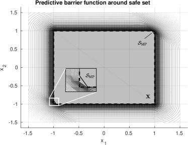
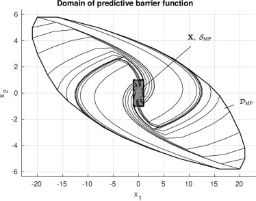
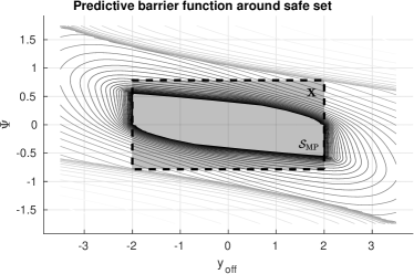
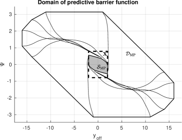
Figure 5: Illustrative example E.1 (top row) and the nonlinear vehicle example according to Section E.2 by projecting onto the states $y_{\mathrm{off}}$ and $\Phi$ (bottom row). Left column: Shown is the state space $\mathbb{X}$ together with predictive safe set $\SS_{\mathrm{PB}}$ as defined in Theorem C.4. Gray contour lines depict level sets of the predictive barrier function $h_{\mathrm{PB}}(x)$ around the safe set $\SS_{\mathrm{PB}}$. Right column: The outer set $\mathcal{D}_{\mathrm{PB}}$ represents the domain of $h_{\mathrm{PB}}(x)$ as defined in (18) with simulated closed-loop recovery trajectories towards the safe set $\SS_{\mathrm{PB}}\subseteq\mathbb{X}$ under application of $u(k)=u^{*}_{0|k}(x(k))$.

Consider the unstable linear system [14]

$$x(k+1)=\begin{bmatrix}1.05&1\\ 0&1\end{bmatrix}x(k)+\begin{bmatrix}1\\ 0.5\end{bmatrix}u(k),$$ (23)

which is subject to state and control constraints $\|x\|_{\infty}\leq 1$ and $\|u\|_{\infty}\leq 1$. We are given a simple stabilizing performance controller of the form $u(k)=K_{p}x(k)$ with $K_{p}=[-0.5592,-0.9445]$ and address recovery of the system from initial state constraint violations $x\notin\mathbb{X}$, which can additionally cause infeasible control inputs $u=K_{p}x\notin\mathbb{U}$.

The constraint tightening is selected as $\Delta_{i}=i\cdot 0.005$ along prediction time steps $i=0,..,19$. To design the corresponding terminal control barrier function according to Assumption 1 and Theorem C.4, we apply the procedure described in Section C.2 with $\mu_{x}=\mu_{u}=0.01$ to obtain $P=\left[\begin{smallmatrix}0.007&0.015\\ 0.015&0.086\end{smallmatrix}\right]$, $K=-[0.062,~{}0.288]$ with corresponding level sets $\gamma_{f}=1$ and $\gamma_{x}=0.0035$. The resulting terminal control barrier function is therefore given by $h_{f}=\max(0,x^{\top}Px-\gamma_{x})$ with domain $\mathcal{D}_{f}=\{x\in\mathbb{R}^{n}:x^{\top}Px\leq 1\}$. The predictive control barrier function problem (9) is implemented using a planning horizon $N=20$ with terminal weight $\alpha_{f}=1000$, satisfying the bound in the proof of Theorem C.4, yielding the domain $\mathcal{D}_{\mathrm{PB}}=\{x\in\mathbb{R}^{n}:h_{\mathrm{PB}}(x)<1000\}$ according to (18).

In Figure 5 (top left), we show the state constraints together with the resulting predictive safe set $\SS_{\mathrm{PB}}=\{x\in\mathbb{R}^{n}:h_{\mathrm{PB}}(x)=0\}$ according to Theorem C.4, i.e. the zero level set of the predictive barrier function $h_{\mathrm{PB}}(x)$ (9) together with logarithmically scaled contour lines of $h_{\mathrm{PB}}(x)$ around $\SS_{\mathrm{PB}}$. Despite the constraint tightening, the safe set $\SS_{\mathrm{PB}}$ covers almost the entire state space, providing a possibly small amount of interference with respect to the linear control law inside the state constraints $\mathbb{X}$.

We demonstrate recovery from infeasible initial conditions in Figure 5 (top right), where we display the enlarged domain $\mathcal{D}_{\mathrm{PB}}$ of $h_{\mathrm{PB}}(x)$ as defined in (18) together with the safe set of the predictive control barrier function $\SS_{\mathrm{PB}}$ and closed-loop system trajectories under application of $u(k)=u^{*}_{0|k}(x(k))$, starting at the boundary of $\mathcal{D}_{\mathrm{PB}}$. As guaranteed by Theorem C.4, all trajectories converge to $\SS_{\mathrm{PB}}$.

While the presented predictive control barrier function method has some fundamental differences compared with the soft constrained approach presented in [14] that is limited to linear systems and provides stability with respect to the origin only, the resulting enlarged region of attraction $\mathcal{D}_{\mathrm{PB}}$ has a similar shape.

E.2 Nonlinear example: Kinematic car model

In this example, the goal is to recover an unsafe state of a kinematic vehicle model from large initial deviations with respect to lateral safety constraints. For the car simulation we consider the dynamics

$$\dot{y}_{\mathrm{off}} =(v_{s}+v)\sin(\Psi)$$ (24)

$$\dot{\Psi} =((v_{s}+v)/L)\tan(\delta)$$ (25)

$$\dot{\delta} =u_{1}$$ (26)

$$\dot{v} =u_{2},$$ (27)

where $y_{\mathrm{off}}$ and $\Psi$ define the offset and relative angle with respect to a centerline, $\delta$ the steering angle, $v$ the relative longitudinal vehicle speed with respect to a target velocity $v_{s}=5~{}\mathrm{[m/s]}$, $u_{1}$ the applied steering rate, and $u_{2}$ the applied acceleration. The physical input limitations are given by $|u_{1}|\leq 1.4$ and $-5\leq u_{2}\leq 2$ as well as $|\delta|\leq 0.35$. The desired safety constraints are defined as $|y_{\mathrm{off}}|\leq 2$, $|\Psi|\leq\pi/4$, and $-4\leq v\leq 5$. Similar to the linear example, we consider recovery of an infeasible initial condition $x\notin\mathbb{X}$.

For the design of the required terminal barrier function $h_{f}$ according to Assumption 1 and Theorem C.4, we proceed as described in Section D by first discretizing the system using Euler forward and a sampling interval of $0.05$ [s]. We select the constraint tightening $\Delta_{i}=i\cdot 0.004$ and linearize around the origin to compute for $\mu_{x}=\mu_{u}=0.1$ the matrix

$$P=\begin{bmatrix}0.30&1.07&0.39&0.00\\ 1.07&5.72&2.54&0.00\\ 0.39&2.54&1.69&0.00\\ 0.00&0.00&0.00&0.20\end{bmatrix},$$

with corresponding controller gain $K=-\left[\begin{smallmatrix}0.28&2.45&1.77&0.00\\ 0.00&0.00&0.00&0.90\end{smallmatrix}\right]$. Application of Step 2 and Step 3 in Section D yield $\gamma_{f}=0.13$ and $\gamma_{x}=0.0108$. The corresponding the terminal control barrier function is given by $h_{f}(x)=x^{\top}Px-\gamma_{x}$ with terminal weight $\alpha_{f}=10^{5}$, satisfying the bound in the proof of Theorem C.4.

In Figure 5 (bottom left), we plot the state constraints together with the resulting predictive safe set $\SS_{\mathrm{PB}}$ with planning horizon $N=50$ for the states $\Psi$ and $y_{\mathrm{off}}$ by setting $v=\delta=0$ together with logarithmically scaled contour lines of $h_{\mathrm{PB}}(x)$ around $\SS_{\mathrm{PB}}$. The safe set $\SS_{\mathrm{PB}}$ touches the lateral constraints only for car headings that do not point away from the center line as expected.

In Figure 5 (bottom right) we display the resulting domain of the predictive control barrier function $h_{\mathrm{PB}}(x)$ as defined in (18), from which we can recover infeasible initial conditions and provide sample closed-loop simulations from the extreme points of $\mathcal{D}_{\mathrm{PB}}$, which all converge to $\SS_{\mathrm{PB}}$ as desired.

Appendix F Conclusion

This paper has addressed the problem of infeasibility of predictive safety filters resulting, e.g., from infeasible initial system conditions or large disturbances. Since a simple softening of the state constraints does not necessarily imply recovery from constraint violations, we proposed a recovery mechanism with an auxiliary feasibility problem using an iterative constraint tightening along the planning horizon together with a terminal safe set, which is required to be a level set of a corresponding discrete-time control barrier function. Asymptotic stability of the feasible set of the original predictive safety filter problem under the proposed algorithm is shown using ideas from control barrier function theory. A principled design procedure for the required components was provided together with numerical examples to demonstrate recovery from constraint violations.

F.1 Lyapunov stability with respect to sets

Consider the discrete-time autonomous system of the form (15) with dynamics $g:\mathbb{R}^{n}\rightarrow\mathbb{R}^{n}$ and initial condition $x(0)=x_{0}$ with $x_{0}\in\mathbb{R}^{n}$. Our goal in this section is to show Lyapunov stability results in terms of a safe set $\SS\subset\mathbb{R}$, e.g. given by (6), which is positively invariant. Following standard stability arguments, the result will be established via a Lyapunov function.

Definition F.1.

Let $\SS,\mathcal{D}\subset\mathbb{R}^{n}$ be non-empty and compact sets with $\SS\subset\mathcal{D}$ and consider a continuous function $V:\mathcal{D}\rightarrow\mathbb{R}$. We call $V(x)$ a locally positive definite (l.p.d.) function around $\SS$ in $\mathcal{D}$ if it holds that

$$\forall x\in\SS:~{}V(x) =0\text{ and}$$ (28a)

$$\forall x\in\mathcal{D}\setminus\SS:~{}V(x) >0.$$ (28b)

$\lhd$

Definition F.2.

Let $\SS,\mathcal{D}\subset\mathbb{R}^{n}$ be non-empty and compact sets with $\SS\subset\mathcal{D}$ and consider a l.p.d. function $V:\mathcal{D}\rightarrow\mathbb{R}$ around $\SS$ in $\mathcal{D}$. If there exists a continuous l.p.d. function $\Delta V(x)$ around $\SS$ in $\mathcal{D}$ such that for all $x\in\mathcal{D}$ the difference inequality

$$V(g(x))-V(x)\leq-\Delta V(x)$$ (29)

holds with respect to system (15), then $V$ is called a Lyapunov function for system (15) with respect to $\SS$ in $\mathcal{D}$. $\lhd$

Using a similar analysis structure as in the case of Lypunov stability analysis with respect to equilibrium points, we can extend existing results to also hold with respect to invariant sets without relying on the existence of lower and upper bounding class $\mathcal{K}$ functions on the Lyapunov function. While these are commonly used in MPC literature, see, e.g., in [11, Appendix B.2], establishing existence of the required class $\mathcal{K}$ functions for (9) would be difficult due to the lack of a positive definite stage cost function with respect to the implicit target set of states $\SS_{\mathrm{PB}}$ as considered in Theorem C.4.

Theorem F.3.

Consider system (15). Let $\SS$ and $\mathcal{D}$ be non-empty and compact sets with $\SS\subset\mathcal{D}$ that are positively invariant for system (15). If there exists a Lyapunov function with respect to $\SS$ in $\mathcal{D}$ for system (15), then $\SS$ is an asymptotically stable set for system (15) in $\mathcal{D}$.

Proof.

The following proof showing (16) is based on [36, Theorem 4.1] with adjustments to account for a discrete-time setting as well as stability w.r.t. a set rather than an equilibrium point. Property (16a): We first consider the case $\epsilon>0$ such that for all $x\in\mathbb{R}^{n}$ with $|x|_{\SS}\geq\epsilon$ it follows $x\notin\mathcal{D}$. Due to forward invariance of $\mathcal{D}$, this case fulfills (16a) by definition for any $x(0)\in\mathcal{D}$.

In the remaining case, i.e. $\epsilon>0$ such that there exists an $x\in\mathbb{R}^{n}$ with $|x|_{\SS}\leq\epsilon$ for which it holds $x\in\mathcal{D}$, we construct a $\delta>0$ in the following such that $|x(0)|_{\SS}<\delta\Rightarrow|x(k)|_{\SS}<\epsilon$ holds for all $k\in\mathbb{N}$. Define

$$V^{-}\coloneqq\min_{|x|_{\SS}\geq\epsilon,~{}x\in\mathcal{D}}V(x),$$ (30)

the existence of which can be verified as follows: From $|x|_{\SS}$ being continuous we have that the pre-image $\{x~{}|~{}|x|_{\SS}\geq\epsilon\}$ is closed, which yields an overall compact subset constraint on $x$ in (30) when intersecting the closed pre-image with the compact set $\mathcal{D}$. Since $V(x)$ is continuous it follows from the extreme value theorem that the minimum $V^{-}$ in (30) exists and since $V(x)$ is l.p.d. around $\SS$ in $\mathcal{D}$ with $\SS\subset\mathcal{D}$ (Definition F.1) it follows that $V^{-}>0$.

Due to continuity of $V$, we can select a $\delta>0$ such that $\left\lVert{x-\bar{x}}\right\rVert<\delta\Rightarrow|V(x)-V(\bar{x})|<V^{-}$ implying for all $\bar{x}\in\mathcal{D}$ such that $|\bar{x}|_{\SS}<\delta$ that $V(\bar{x})<V^{-}$.

For an initial condition $|x(0)|_{\SS}<\delta$ and $x(0)\in\mathcal{D}$ we therefore have from $V(x(0))<V^{-}$ together with the fact that $V(x(k))$ is non-increasing for $k\in\mathbb{N}$ (Definition F.2) and positive invariance of $\mathcal{D}$ and $\SS$ that $V(x(k))<V^{-}$ holds for all $k\in\mathbb{N}$.

Assume there exists a time step $\bar{k}\in\mathbb{N}$ such that $|x(\bar{k})|_{\SS}\geq\epsilon$. By construction of $V^{-}$ it follows $V(x(\bar{k}))\geq V^{-}$, which is a contradiction to the statement $V(x(k))<V^{-}$ above and therefore proves property (16a).

Property (16b): Compared to the first part of this proof, convergence can be shown along the lines of the proof of [36, Theorem 4.1]. Let $x(0)\in\mathcal{D}$. As established above, the sequence $V(x(k))$ is non-increasing for $k>0$ and $V$ is continuous on the bounded set $\mathcal{D}$, implying that it will converge, i.e. $\lim_{k\rightarrow\infty}V(x(k))=\alpha$ with $\alpha\geq 0$.

For a proof by contradiction, select an $\alpha>0$ such that there exists a $x\in\mathcal{D}$ implying $V(x)=\alpha$ and define $\mathcal{A}\coloneqq\{x\in\mathcal{D}:V(x)\leq\alpha\}$. Due to continuity of $V$, we can select a $\beta>0$ such that $|x|_{\SS}<\beta$ implies $V(x)<\alpha$. It follows that the set $\mathcal{B}\coloneqq\{x\in\mathcal{D}:|x|_{\SS}<\beta\}$ with $\beta>0$ satisfies $\mathcal{B}\subset\mathcal{A}$.

Since $V(x(k))$ is monotonically decreasing to $\alpha$ by assumption (Definition F.2) it holds that $V(x(k))\geq\alpha$ for all $k>0$, and therefore we have $x(k)\notin\mathcal{B}$ for all $k>0$. By excluding the possibility of $x(k)\in\mathcal{B}$ for $\alpha>0$, we can locally define the smallest decrease

$$-\gamma=\max_{x\in\mathcal{D},|x|_{\SS}\geq\beta}-\Delta V(x)$$ (31)

with $\Delta V$ according to (29), which is strictly less than zero by assumption (Definition F.2). Furthermore, $\gamma$ is bounded since $\Delta V$ is continuous and $\mathcal{D}$ is compact. Note that (31) always has a feasible suboptimal solution given by $-\Delta V(x(0))$. Forward invariance of $\mathcal{D}$ allows us to use the worst-case decrease from above to obtain

$$V(x(k)) =V(x(k-1))+V(x(k))-V(x(k-1))$$

$$=V(x(0))+\sum_{i=0}^{k-1}V(x(i+1))-V(x(i))$$

$$\leq V(x(0))-\sum_{i=0}^{k-1}\Delta V(x(i))$$

$$\leq V(x(0))-(k-1)\gamma.$$

Since $\gamma>0$ there exists a finite $\bar{k}$ such that $V(x(0))-(\bar{k}-1)\gamma<0$ and therefore $V(x(\bar{k}))<0$, yielding a contradiction for any $x(0)\in\mathcal{D}$. We can therefore select $\bar{\delta}=\max_{x\in\mathcal{D}}|x|_{\SS}$ with $\bar{\delta}>0$ and $\bar{\delta}<\infty$ since $\SS\subset\mathcal{D}$ and $\mathcal{D}$ is compact, proving the desired result. ∎

F.2 Proof of Theorem C.2 (Control barrier functions)

We prove this result by showing invariance of $\SS$ (Property 1) first, followed by asymptotic stability of $\SS$ (Property 2).

Proof.

Property 1: From Definition C.1, (14) it directly follows for any $x(0)\in\SS$ with $u(k)=\kappa(x(k))\in K_{\mathrm{CBF}}^{2}(x)$ that $h(x(k))\leq 0$ implies $h(x(k+1))\leq 0$ and therefore by induction we have that $x(0)\in\SS$ implies $x(k)\in\SS$ for all $k>0$, which proves the desired property.

Property 2: Define $V:\mathcal{D}\rightarrow\mathbb{R}$ as $V(x)=\max(0,h(x))$, which is continuous due to continuity of $h$ and l.p.d. around $\SS$ in $\mathcal{D}$ according to Definition F.1 by construction of $\SS$. In the following, we show that for any control law $\kappa$ with $\kappa(x)\in K_{\mathrm{CBF}}(x)$ according to Definition C.1, it follows that $V$ is a Lyapunov function for the closed-loop system (1) under $u(k)=\kappa(x(k))$ with respect to $\SS$ in $\mathcal{D}$. The corresponding decrease can be bounded through

$$\Delta V(x)=\max(0,\min(\Delta h(x),V(x))).$$ (32)

Since max/min operations preserve continuity properties, it follows that $\Delta V(x)$ is continuous. Furthermore, (32) is positive definite w.r.t. $\SS$ in $\mathcal{D}$ since $x\in\SS$ implies

$$\max(0,\underbrace{\min(\underbrace{\Delta h(x)}_{\in\mathbb{R}},\underbrace{V(x)}_{=0})}_{\leq 0})=0$$

and $x\in\mathcal{D}\setminus\SS$ implies

$$\max(0,\underbrace{\min(\underbrace{\Delta h(x)}_{>0},\underbrace{V(x)}_{>0})}_{>0})>0.$$

Lastly, it remains to verify that the required decrease condition, i.e., Property 2 holds. To this end, we distinguish the following three cases, which are possible due to invariance of $\SS$ and $\mathcal{D}$:

1. $x(k)\in\SS\land x(k+1)\in\SS$:

   $$\underbrace{V(x(k+1))}_{=0}-\underbrace{V(x(k))}_{=0}$$

   $$\leq-\max(0,\underbrace{\min(\underbrace{\Delta h(x(k))}_{\in\mathbb{R}},\underbrace{V(x(k))}_{=0})}_{\leq 0})=0.$$

2. $x(k)\in\mathcal{D}\setminus\SS\land x(k+1)\in\mathcal{D}\setminus\SS$: Notice that due to $h(x(k+1))>0$ we have $h(x(k+1))-h(x(k))\leq-\Delta h(x(k))\Rightarrow h(x(k))\geq\Delta h(x(k))$ in this case, implying

   $$\underbrace{V(x(k+1))}_{=h(x(k+1))}-\underbrace{V(x(k))}_{=h(x(k))}$$

   $$\leq-\max(0,\underbrace{\min(\underbrace{\Delta h(x(k))}_{>0},\underbrace{h(x(k))}_{\geq\Delta h(x(k))})}_{=\Delta h(x(k))>0})=-\Delta h(x(k)).$$

3. $x(k)\in\mathcal{D}\setminus\SS\land x(k+1)\in\SS$: Notice that due to $h(x(k+1))\leq 0$ it follows $\Delta h(x(k))\geq h(x(k))=V(x(k))$ in this case and we have

   $$\underbrace{V(x(k+1))}_{=0}-V(x(k))$$

   $$\leq-\max(0,\underbrace{\min(\underbrace{\Delta h(x(k))}_{>0},\underbrace{V(x(k))}_{\leq\Delta h(x(k))})}_{=V(x(k))>0})\leq-\underbrace{V(x(k))}_{>0}.$$

Since all the cases above are guaranteed to be true and satisfy Property 2, the desired statement follows directly from Theorem F.3. ∎

F.3 Technical lemmas for the proof of Theorem C.4

Lemma F.1.

If the conditions in Theorem C.4 hold, then the minimum (9) exists for all $x\in\mathbb{R}^{n}$.

Proof.

The constrained optimization problem (9) can equally be written in the condensed form

$$\inf_{u_{i}\in\mathbb{U}}~{} \alpha_{f}\max(0,h_{f}(f(..f(f(x,u_{0}),u_{1}),..)))$$

$$+\sum_{i=0}^{N-1}\left\lVert{\max(0,c(f(..f(f(x,u_{0}),u_{1}),..))+\Delta_{i}\mathbbm{1},0)}\right\rVert,$$

with $x_{1|k}=f(x,u_{0|k})$, $x_{2|k}=f(f(x,u_{0|k}),u_{1|k})$, .., $\xi_{i|k}=\max(0,c(x_{i|k}))$ for all $i=0,..,N-1$, and $\xi_{N|k}=\max(0,h_{f}(x_{N|k}))$. Since compositions, sums, and the maximum of continuous functions yield continuous functions and $h_{f}$, $c$, and $f$ are assumed to be continuous on $\mathbb{R}^{n}$, it follows that the objective is continuous on $\mathbb{R}^{n}$. In addition, the input space $\mathbb{U}$ is assumed to be compact, allowing us to apply the Weierstrass Extreme Value Theorem [11, Proposition A.7], which implies that the minimum exists for all $x\in\mathbb{R}^{n}$ and therefore the proof is complete. ∎

Lemma F.2.

If the conditions in Theorem C.4 hold, then it follows that $\mathcal{D}_{\rho}=\{x\in\mathbb{R}^{n}|h_{\mathrm{PB}}(x)\leq\rho\}\subseteq\mathbb{X}_{0}(\mathbbm{1}\rho)$ with $\rho>0$ and $\mathbb{X}_{0}(\mathbbm{1}\rho)$ according to (12).

Proof.

For any $x\in\mathcal{D}_{\rho}$ it follows that the objective function (9a) implies that $\lVert{\xi_{0|k}^{*}}\rVert\leq\rho$ and it must therefore hold that $x=x_{0|k}\in\mathbb{X}_{0}(\mathbbm{1}\rho)$, which proves the desired statement. ∎

Lemma F.3.

Let the conditions in Theorem C.4 hold and consider a state $x\in\mathcal{D}_{\rho}$ with $\mathcal{D}_{\rho}=\{x\in\mathbb{R}^{n}|h_{\mathrm{PB}}(x)\leq\rho\}$, $\rho\geq 0$ and input sequence $\{u_{i|k}\}_{i=0}^{N-1}\in\mathbb{U}^{N-1}$. Define a corresponding state sequence $x_{0|k}\coloneqq x$ and $x_{i+1|k}\coloneqq f(x_{i|k},u_{i|k})$ for $i=0,..,N-1$ and slack sequence $\xi_{i|k}\coloneqq\max(0,c(x_{i|k})+\Delta_{i}\mathbbm{1})$ for $i=0,..,N-1$, $\xi_{N|k}\coloneqq\max(0,h_{f}(x_{N|k}))$. For every $\rho\geq 0$, there exists a compact set $\mathbb{Z}_{\rho}$ such that for all $x\in\mathcal{D}_{\rho}$ and $\{u_{i|k}\}_{i=0}^{N-1}\in\mathbb{U}^{N-1}$ it holds that $(\{x_{i|k}\}_{i=0}^{N},\{\xi_{i|k}\}_{i=0}^{N}\})\in\mathbb{Z}_{\rho}$.

Proof.

From Lemma F.2, we know that $x\in\mathcal{D}_{\rho}$ will be contained in the compact set $\mathbb{X}_{0}(\mathbbm{1}\rho)$. Since the dynamics are continuous and the input space is compact, it follows that the prediction mapping of the outer bounding initial set $\mathbb{X}_{0}(\mathbbm{1}\rho)$ that contains the states $\{x_{i|k}\}_{i=0}^{N}$ will be compact. By noting that a feasible slack sequence for any state sequence $\{x_{i|k}\}_{i=0}^{N}$ is given by the continuous mapping $\xi_{i|k}=\max(0,c(x_{i|k}))$ and $\xi_{N|k}=\max(0,c(x_{N|k}))$, it follows that a valid set of slack sequences corresponding to the compact set of possible states sequences will be compact and therefore the proof is complete. ∎

[]Kim P. Wabersich received a BSc. and MSc. degree in engineering cybernetics from the University of Stuttgart in Germany in 2015 and 2017, respectively. He completed his doctoral studies at ETH Zurich in 2021 and is currently a postdoctoral researcher with the Institute for Dynamic Systems and Control (IDSC) at ETH Zurich. During his studies, he was a research assistant at the Machine Learning and Robotics Lab (University of Stuttgart) and the Daimler Autonomous Driving Research Center (Böblingen, Germany and Sunnyvale, CA, USA). His research interests include learning-based model predictive control and safe model-based reinforcement learning. []Melanie N. Zeilinger is an Assistant Professor at ETH Zurich, Switzerland. She received the Diploma degree in engineering cybernetics from the University of Stuttgart, Germany, in 2006, and the Ph.D. degree with honors in electrical engineering from ETH Zurich, Switzerland, in 2011. From 2011 to 2012 she was a Postdoctoral Fellow with the Ecole Polytechnique Federale de Lausanne (EPFL), Switzerland. She was a Marie Curie Fellow and Postdoctoral Researcher with the Max Planck Institute for Intelligent Systems, Tübingen, Germany until 2015 and with the Department of Electrical Engineering and Computer Sciences at the University of California at Berkeley, CA, USA, from 2012 to 2014. From 2018 to 2019 she was a professor at the University of Freiburg, Germany. Her current research interests include safe learning-based control, as well as distributed control and optimization, with applications to robotics and human-in-the-loop control.

References

- [1] D. Seto, B. Krogh, L. Sha, and A. Chutinan, “The simplex architecture for safe on-line control system upgrades,” in Proceedings of the American Control Conference, vol. 6. IEEE, 1998, pp. 3504–3508.
- [2] A. D. Ames, S. Coogan, M. Egerstedt, G. Notomista, K. Sreenath, and P. Tabuada, “Control barrier functions: Theory and applications,” 2019 18th European Control Conference, ECC 2019, pp. 3420–3431, 2019.
- [3] M. Chen and C. J. Tomlin, “Hamilton–Jacobi Reachability: Some Recent Theoretical Advances and Applications in Unmanned Airspace Management,” Annual Review of Control, Robotics, and Autonomous Systems, vol. 1, no. 1, pp. 333–358, 2018.
- [4] T. Gurriet, M. Mote, A. D. Ames, and E. Feron, “An Online Approach to Active Set Invariance,” in Proceedings of the IEEE Conference on Decision and Control, vol. 2018-Decem, 2019, pp. 3592–3599.
- [5] T. Mannucci, E. J. Van Kampen, C. De Visser, and Q. Chu, “Safe Exploration Algorithms for Reinforcement Learning Controllers,” IEEE Transactions on Neural Networks and Learning Systems, vol. 29, no. 4, pp. 1069–1081, 2018.
- [6] K. P. Wabersich, L. Hewing, A. Carron, and M. N. Zeilinger, “Probabilistic model predictive safety certification for learning-based control,” IEEE Transactions on Automatic Control, pp. 1–1, 2021.
- [7] K. P. Wabersich and M. N. Zeilinger, “A predictive safety filter for learning-based control of constrained nonlinear dynamical systems,” Automatica, vol. 129, p. 109597, 2021. [Online]. Available: https://www.sciencedirect.com/science/article/pii/S0005109821001175
- [8] S. Li and O. Bastani, “Robust model predictive shielding for safe reinforcement learning with stochastic dynamics,” in 2020 IEEE International Conference on Robotics and Automation (ICRA). IEEE, 2020, pp. 7166–7172.
- [9] K. P. Wabersich and M. N. Zeilinger, “Linear model predictive safety certification for learning-based control,” in 2018 IEEE Conference on Decision and Control (CDC). IEEE, 2018, pp. 7130–7135.
- [10] T. Gurriet, M. Mote, A. Singletary, P. Nilsson, E. Feron, and A. D. Ames, “A Scalable Safety Critical Control Framework for Nonlinear Systems,” IEEE Access, pp. 1–1, 2020.
- [11] J. B. Rawlings, D. Q. Mayne, and M. M. Diehl, Model Predictive Control: Theory, Computation, and Design, 2nd ed. Nob Hill Publishing, 2017.
- [12] E. C. Kerrigan and J. M. Maciejowski, “Soft Constraints And Exact Penalty Functions In Model Predictive Control,” in Control 2000 Conference. Citeseer, 2000.
- [13] Z. Marvi and B. Kiumarsi, “Safe reinforcement learning: A control barrier function optimization approach,” International Journal of Robust and Nonlinear Control, no. May, pp. 1–18, 2020.
- [14] M. N. Zeilinger, M. Morari, and C. N. Jones, “Soft Constrained Model Predictive Control With Robust Stability Guarantees,” IEEE Transactions on Automatic Control, vol. 59, no. 5, pp. 1190–1202, 2014.
- [15] D. Limon, T. Alamo, D. Raimondo, D. M. De La Peña, J. Bravo, A. Ferramosca, and E. Camacho, “Input-to-state stability: a unifying framework for robust model predictive control,” in Nonlinear model predictive control. Springer, 2009, pp. 1–26.
- [16] A. G. Wills and W. P. Heath, “Barrier function based model predictive control,” Automatica, vol. 40, no. 8, pp. 1415–1422, 2004.
- [17] C. Feller and C. Ebenbauer, “A stabilizing iteration scheme for model predictive control based on relaxed barrier functions,” Automatica, vol. 80, pp. 328–339, 2017. [Online]. Available: http://dx.doi.org/10.1016/j.automatica.2017.02.001
- [18] A. Domahidi, A. U. Zgraggen, M. N. Zeilinger, M. Morari, and C. N. Jones, “Efficient interior point methods for multistage problems arising in receding horizon control,” in 51st IEEE Conference on Decision and Control (CDC), Dec 2012, pp. 668–674.
- [19] R. Verschueren, G. Frison, D. Kouzoupis, N. van Duijkeren, A. Zanelli, B. Novoselnik, J. Frey, T. Albin, R. Quirynen, and M. Diehl, “Acados: a Modular Open-Source Framework for Fast Embedded Optimal Control,” 2019. [Online]. Available: http://arxiv.org/abs/1910.13753
- [20] Z. Marvi and B. Kiumarsi, “Safety Planning Using Control Barrier Function: A Model Predictive Control Scheme,” in 2019 IEEE 2nd Connected and Automated Vehicles Symposium (CAVS), 2019, pp. 1–5.
- [21] Z. Wu, F. Albalawi, Z. Zhang, J. Zhang, H. Durand, and P. D. Christofides, “Control Lyapunov-Barrier Function-Based Model Predictive Control of Nonlinear Systems,” in 2018 Annual American Control Conference (ACC), 2018, pp. 5920–5926.
- [22] J. Zeng, B. Zhang, and K. Sreenath, “Safety-critical model predictive control with discrete-time control barrier function,” arXiv, 2020.
- [23] R. Grandia, A. J. Taylor, A. Singletary, M. Hutter, and A. D. Ames, “Nonlinear model predictive control of robotic systems with control lyapunov functions,” in Proceedings of Robotics: Science and Systems XVI. Robotics: Science and Systems Foundation, 2020.
- [24] L. Hewing, K. P. Wabersich, M. Menner, and M. N. Zeilinger, “Learning-Based Model Predictive Control: Toward Safe Learning in Control,” Annual Review of Control, Robotics, and Autonomous Systems, vol. 3, no. 1, pp. annurev–control–090 419–075 625, May 2020.
- [25] H. Chen and F. Allgöwer, “A quasi-infinite horizon nonlinear model predictive control scheme with guaranteed stability,” Automatica, vol. 34, no. 10, pp. 1205 – 1217, 1998.
- [26] G. Di Pillo and L. Grippo, “Exact penalty functions in constrained optimization,” SIAM Journal on Control and Optimization, vol. 27, no. 6, pp. 1333–1360, 1989.
- [27] M. Ohnishi, L. Wang, G. Notomista, and M. Egerstedt, “Barrier-Certified Adaptive Reinforcement Learning With Applications to Brushbot Navigation,” IEEE Transactions on Robotics, vol. 35, no. 5, pp. 1186–1205, 2019.
- [28] W. Rudin et al., Principles of mathematical analysis. McGraw-hill New York, 1964, vol. 3.
- [29] J. F. Fisac, A. K. Akametalu, M. N. Zeilinger, S. Kaynama, J. Gillula, and C. J. Tomlin, “A General Safety Framework for Learning-Based Control in Uncertain Robotic Systems,” IEEE Transactions on Automatic Control, vol. 64, no. 7, pp. 2737–2752, 2019.
- [30] S. Boyd, L. El Ghaoui, E. Feron, and V. Balakrishnan, Linear Matrix Inequalities in System and Control Theory. SIAM, 1994.
- [31] C. G. E. Boender and H. E. Romeijn, Stochastic Methods. Boston, MA: Springer US, 1995, pp. 829–869. [Online]. Available: https://doi.org/10.1007/978-1-4615-2025-2_15
- [32] J. Löfberg, “Yalmip : A toolbox for modeling and optimization in matlab,” in In Proceedings of the CACSD Conference, Taipei, Taiwan, 2004.
- [33] M. Herceg, M. Kvasnica, C. Jones, and M. Morari, “Multi-Parametric Toolbox 3.0,” in Proc. of the European Control Conference, Zürich, Switzerland, July 17–19 2013, pp. 502–510, http://control.ee.ethz.ch/ mpt.
- [34] J. A. E. Andersson, J. Gillis, G. Horn, J. B. Rawlings, and M. Diehl, “CasADi – A software framework for nonlinear optimization and optimal control,” Mathematical Programming Computation, 2018.
- [35] L. T. Biegler and V. M. Zavala, “Large-scale nonlinear programming using ipopt: An integrating framework for enterprise-wide dynamic optimization,” Computers & Chemical Engineering, vol. 33, no. 3, pp. 575–582, 2009.
- [36] H. K. Khalil and G. J. W., Nonlinear Systems, 2001, vol. 3.