Rational Dynamic Price Model for Demand Response Programs in Modern Distribution Systems

Abstract

Demand response (DR) refers to change in electricity consumption pattern of customers during on-peak hours in lieu of financial gains to reduce stress on distribution systems. Existing dynamic price models have not provided adequate success to price-based demand response (PBDR) programs. It happened as these models have raised typical socio-economic problems pertaining to cross-subsidy, free-riders, social inequity, assured profit of utilities, financial gains and comfort of customers, etc.This paper presents a new dynamic price model for PBDR in distribution systems which aims to overcome some of the above mentioned problems of the existing price models. The main aim of the developed price model is to overcome the problems of cross-subsidy and free-riders of the existing price models for widespread acceptance, deployment and efficient utilization of PBDR programs in contemporary distribution systems. Proposed price model generates demand-linked price signal that imposes different price signals to different customers during on-peak hours and remains static otherwise. This makes proposed model a class apart from other existing models. The novelty of the proposed model lies in the fact that the financial benefits and penalties pertaining to DR are self-adjusted among customers while preserving social equity and profit of the utility. Such an ideology has not been yet addressed in the literature. Detailed investigation of application results on a standard test bench reveals that the proposed model equally cares regarding the interests of both customers and utility. For economic assessment, a comparison of the proposed price model with the existing pricing models is also performed.

Nomenclature

l]p35pt p200pt $P^{\text{MCP}}(t)$	Market clearing price at $t$th state.
$D(i,j,t)$	Demand of jth customer of $i$th category during $t$th state.
$N_{s}$	Total number of customers in a particular category.
$k_{p}(i)$	Profit factor of utility for $i$th category of customers.
$P(i,j,t)$	Unit price of $j$th customer of $i$th category during the state $t$.
$\alpha(i,t)$	Constant of demand proportionality at $t$th state.
$N_{\text{cat}}$	Total number of customer categories.
$N_{\text{on}}$	Total number of on-peak hours.
$N_{\text{off}}$	Total number of off-peak hours.
$T_{\text{on-peak}}$	Duration of on-peak hours.
$T_{\text{off-peak}}$	Duration of off-peak hours.
$t$	Duration of $t$th state.
$i$	Type of customer category.
$j$	Type of customer in a particular category.
$T$	Set of system states.
$\Omega_{\text{on}}$	Set of on-peak hours.
$\Omega_{\text{off}}$	Set of off-peak hours.
$\Omega_{\text{cat}}$	Set of customer categories.
$\Omega_{s}$	Set of customers in a particular category.

I Introduction

The electricity markets around the globe are undergoing fast transformation. In the emerging electricity markets, the dynamic pricing has assumed significant importance. The conventional electricity markets generally offer two types of pricing structures namely, fixed-rate pricing or flat pricing and block-rate pricing. In fixed price structure, the electricity price remains same irrespective of the energy consumption whereas in block-rate pricing structure the per unit rate of electricity changes with the energy consumption slabs. However, the cost of electricity generation is neither fixed nor changes with slabs. The cost of electricity during peak demand hours are much higher than that of during off-peak hours. And so under the conventional pricing structure, the traditional market takes into account the spot pricing risk into the cost-to-serve customers, thereby making them to pay a premium to hedge against financial losses [1, 2]. Moreover, cross-subsidy occurs as the cost-causers are not contributing proportionately towards the generation cost, as a result social equity hampers. The generation-cost and consumption-cost gap is dynamic in nature. This leads to emergence of demand response (DR) coupled dynamic pricing in the electricity-market design. The demand response is the change of electricity consumption pattern of the consumers in response to dynamic pricing. The DR may provide several techno-economic and social benefits by changing the consumption pattern of end users in lieu of financial incentives. The annual report of the U.S. DoE and Federal Energy Regulatory Commission (FERC) on demand response (DR) describes in depth the benefits of DR in electricity markets, and carries out a systematic analysis for DR implementation [3, 4, 5, 6]. The effective implementation of DR and larger participation of end customer in DR may play a bigger role in deferring capital investments in generation expansion, to enhance system efficiency and security, to create fairness in retail pricing, to increase electricity market efficiency, protect market players from spot price volatility risks, provide potential environmental benefits, etc.[7, 8, 9, 10, 3, 4, 5, 6].

In literature several price-based DR (PBDR) programs have been reported [11, 12, 13, 14]. In the price-based DR, different types of dynamic pricing models are used some of these may include real time pricing (RTP), time of use (TOU) pricing, critical peak pricing (CPP) and peak time rebate (PTR) [11, 12, 13, 14]. In RTP, the price signal changes in accordance with the whole sale electricity price, usually recieved a day ahead. The TOU offers two or three-level pricing signals during the day thus provide more flexibility to consumers than RTP. The CPP is same as that of the TOU, but it offers very high price signals during certain critical hours/days. The PTR is also similar to CPP, but it provides cash rebate for demand reduction unlike peak time pricing for consumption. The CPP and the PTR price signals have limited operation time as they are employed for only critical situations of short durations. The RTP offers complex pricing structure but has proven to be most efficient and capable to bring many benefits to customers and utilities in the form of reduced bills and peak load reduction [15, 16, 17]. However, it requires advanced ICT [13] and exposes low consumption consumers to spot pricing risk [1], besides more responsiveness of the customers. The TOU is characterized by simplified energy pricing structure thus encourages permanent load shifting without using advanced ICT [18]. The TOU also provide efficient risk management, enhanced market efficiency, reduced billing, improved integration of DERs [19, 20, 21, 22, 23, 24, 25, 26, 27, 18]. Moreover, financial incentives offered under TOU pricing signal can act as a feasible alternative to RTP signal [13]. A trade-off between risk and reward in dynamic pricing signals from the customers’ perspective is presented in Ref. [28, 18]. The authors illustrated that more the dynamic nature of a pricing signal less will be the risk aversion and more will be the economic efficiency, and vice-versa. Among all dynamic pricing signals, TOU provides compromising results across the spectrum of risk-reward trade-off, therefore, is accepted by majority of the customers. However, TOU pricing is not free from free-riders and cross-subsidy. In Ref. [29], a demand response exchange scheme is employed for the elimination of free-rider problem. Another congenital issue with dynamic pricing is the rebound effect [30, 31, 32, 33] that may occur under highly fluctuating price signals in which customers dramatically delay consumption pattern to maximize financial gains and/or to avoid a peak, but cause a new peak while trying to satisfy the delayed demand after the DR event ends. The pronounced rebound effect may even defeat the purpose of the PBDR program. There are several other key issues in PBDR such as social equity [1], ineffective pricing models [1, 34, 35], regulatory/market coordination [36, 7], customer behavior [11], customer fears of price volatility [37], etc. which may overcast the successful implementation of PBDRs.

The existing PBDR programs have not gained much popularity perhaps due to non-active participation of high-consumption customers in DR programs (DRPs) due to their financial flexibility. These high consumption non-participating consumers, enjoying the benefits offered by the active participation of low-income customers, are referred to as free-riders [38, 29, 39]. These free-riders may cause substantial distortions of a market [40]. Usually, the most prominent free-riders are responsible for cross-subsidy thus hampers social equity and causes unjustified allocation of benefits to other customers. The success of PBDR programs depends upon many factors such as the risk aversion of utilities, better understanding, social equity, fair and transparent allocation of DR benefits to customers, etc. A PBDR program therefore should overcome typical limitations of existing DRPs, viz. free-rider problem, cross-subsidy and rebound effect, while preserving the benefits of customers and social equity and should also offset risk aversion of utilities.

This paper proposes a novel demand contribution based dynamic price model for the successful implementation of PBDR in modern distribution systems which aims to overcome the shortcomings of existing pricing models. The proposed price model generates a demand-linked price signal (DLPS) during on-peak hours of the day. The DLPS provides dynamic price signal in proportion to customer’s share in peak demand. Proposed price model is unique as it imposes different price signals to different customers during on-peak hours and remains static otherwise. DLPS varies with both time and customers. The proposed modeling intends to be free from cross-subsidy and free-rider problems, mitigate rebound effect, and fairly allocate DR benefits with social equity while preserving the profit of the utilities. Proposed price model is thoroughly implemented and analyzed on a benchmark 33-bus test distribution system and the application results obtained are presented and compared.

II Motivations and the Proposed Pricing Model

In the existing PBDR programs, the free-riders avail undue DR benefits and may introduce cross-subsidy by not reducing their demand during on-peak hours, thus severely affects due DR benefits to other customers. The problem worsens in the presence of big free-riders. The root cause of this problem is that the existing dynamic price signals are linked, in some way, with the total demand of the distribution system rather than individual demand. Although the price-based DR is intended to change individual’s demand. The billing of customers has a reflection of both individual’s demand and dynamic price signal generated on account of total demand. There is no discrimination on the basis of participation of individual consumers in DR. The inconsistency exists between the price signal and DR benefits. Due to this inconsistency the DR benefits are not judiciously allocated among customers. Although the customers participating pro-actively in DR are responsible for the reduced price signal. The benefits pass on to all consumers irrespective of their participation level in DR. This ultimately results in cross-subsidy and free-rider problems. Therefore, the price-signal should also take into account the individual demand of the customers for effective implementation of PBDR.

Usually, customers prefer TOU on account of its simplicity and less price responsiveness, whereas the utilities prefer RTP owing to risk aversion. This is because the customers can focus on a dynamic price signal, at the most, for few hours while considering their loss of comfort, habits or the mindset. The spot pricing volatility is the main reason behind the preferential choice of RTP by utilities, but it requires almost round-the-clock attention of customers. However, only few hours (on-peak hours) are of significant importance for utilities from techno-economic aspects. Therefore, a dynamic price signal that capture the static nature of pricing during off-peak hours and provides dynamic price signals in proportion to customer’s share in peak demand may be a better alternative to intact benefits of both customers and utility. A graphical representaion of the proposed pricing structure for $N_{s}$ customers along with existing pricing signals is shown in Fig. 1.

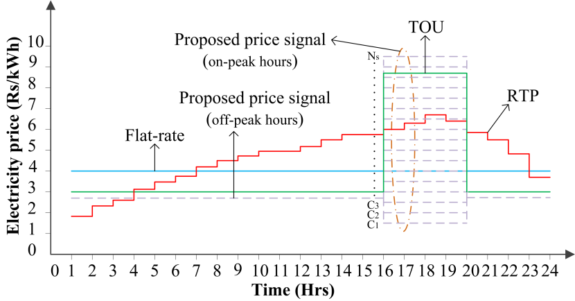
Figure 1: Graphical representation of the proposed pricing structure.

III Mathematical Modeling of the Proposed Pricing Structure

The mathematical modeling of the proposed dynamic pricing structure is based upon economic balance equation (EBE). EBE equalizes total purchase cost of electricity and the revenue generated for each system state considering demand of individual customer and market clearing price (MCP) while ensuring assured profit of the utility from the purchase and sale of electricity. In this paper, a separate EBE is suggested for each category of customers, and is exclusively modeled for on-peak and off-peak hours. For a particular category, proposed price modeling generates different dynamic price signals to different customers only during the on-peak hours.

III-A Dynamic Price Signal for On-Peak Hours

The EBE for the $j$th customer of $i$th category for the state $t$ can be expressed as

The left and right hand side of the equation (1) denotes the purchase cost of electricity, including assured profit, and the corresponding revenue generated from electricity sale for the state $t$ respectively. $k_{p}(i)$ is the profit factor pre-established by the utility for $i$th category of customers and is included in order to ensure profit of the utility. The profit factor may be set different for different categories of customers considering social equity.

For proportional contributory demand, the dynamic price signal can be defined as

$$P(i,j,t)=\alpha(i,t)\frac{D(i,j,t)}{\sum\limits_{j=1}^{{{N}_{s}}}{D(i,j,t)}};\forall i\in{{\Omega}_{\text{cat}}},j\in{\Omega_{s}},t\in{{\Omega}_{\text{on}}}$$ (2)

where, $\alpha(i,t)$ is a constant for demand proportionality that holds during the state $t$ for each customer belonging to $i$th category. Substituting (2) into (1) yields

Using (3) and (2), we get

Equation (4) shows that the dynamic price signal proposed for the $j$th customer of $i$th category during the state $t$ considers profit factor, customer’s demand, demand contribution factor and MCP. Similarly, the price of other category of customers can also be determined. The dynamic price signal defined by (4) provides economic balance for the customers of $i$th category at $t$th state as below:

Equation (5) can be extended for all categories of customers for state $t$ and for the interval $T_{\text{on-peak}}$ by the following equations, respectively.

III-A1 Sensitivity Analysis

Using (4), let

A real distribution system has large number of customers in each category, say residential, industrial, and commercial, etc. or some other consumption-based categories. The equation (8) then can be safely approximated as

A comparison of (3) with (10) yields

$$\alpha(i,t)=\zeta(i,j,t)\sum\limits_{j=1}^{{{N}_{s}}}{D(i,j,t)};\forall i\in{{\Omega}_{\text{cat}}},j\in{\Omega_{s}},t\in{\Omega}_{\text{on}}$$ (11)

Using (11) and (2), it can be shown that

$$\frac{\partial D(i,j,t)}{D(i,j,t)}=\frac{\partial P(i,j,t)}{P(i,j,t)};\forall i\in{{\Omega}_{\text{cat}}},j\in{\Omega_{s}},t\in{\Omega}_{\text{on}}$$ (12)

Equation (12) reveals that the proposed price model imposes the same percentage change in the price signal as that of the percentage change in customer’s demand, and that too with the same sign.

III-B Price Signal for Off-Peak Hours

The EBE for the off-peak period ($T_{\text{off-peak}}$) is defined as

The cost of electricity purchase, including assured profit, and revenue from its sale during the off-peak period are respectively shown in the left and right part of (13). In the off-peak period, the unit price is kept same for all the customers belonging to given category. The unit price to all $i$th category customers during the state $t$ is given by

Proposed model delivers price signals given by (4) and (14) which are based upon independent balancing of EBEs defined by (1) and (13), respectively. Therefore, ensures profit of utility over the day and also addresses social equity by taking suitable values of $k_{p}(i)$ for different categories of customers. The simulation results achieved while employing the proposed price model for on-peak hours for a single state $t$ are discussed in the coming section.

IV Simulation Results

In this section, the proposed pricing model is investigated on 12.66 kV, 33-bus benchmark test distribution system [41]. For this system, the nominal active and reactive load demands are 3.715 MW and 2.30 MVar, respectively. The power losses and minimum node voltage at nominal loading are 202.67 kW and 0.9131p.u. respectively.

IV-A Case Study Data and Validation of the Proposed Pricing Model

A sample day is considered to be composed of 24 states each of the duration 1 Hr. The period from 18:00 Hrs to 23:00 Hrs is assumed to be peak demand period and the remaining period is taken as off-peak hours, as in [42]. The system buses are arbitrarily divided into three categories, viz. residential (N2–N15), commercial (N16–N22, N30–N33) and industrial (N23–N29) as suggested in [43]. A total 177 customers are assumed which are divided as 23 industrial (I1–I23), 106 residential (R1–R106) and 48 commercial (C1–C48) customers. The detail of the customers’ loading is given in Appendix Appendix. It is also assumed that all customers are participating in DRP. The load demand and MCP profiles considered for the sample day are taken from [42] and shown in Fig. 2. The profit factor $k_{p}$ for a particular customer’s category is decided by the utility keeping in view its assured profit. The profit factor for industrial, residential and commercial customers in the present study are assumed as 1.01, 1.03 and 1.02, respectively. In other words, a profit of 1%, 3% and 2% are expected on the sale of energy to industrial, residential and commercial customers respectively.

TABLE I: Results of the proposed dynamic price signal for base case

Customer No.	LD	UP	Customer No.	LD	UP	Customer No.	LD	UP
I1	40	3.22	I9	30	2.41	I17	30	2.41
I2	50	4.02	I10	42	3.38	I18	60	4.82
I3	46	3.70	I11	54	4.34	I19	25	2.01
I4	54	4.34	I12	62	4.99	I20	35	2.81
I5	65	5.23	I13	68	5.47	I21	40	3.22
I6	75	6.03	I14	74	5.95	I22	38	3.06
I7	88	7.07	I15	90	7.24	I23	42	3.38
I8	92	7.40	I16	30	2.41	LD: load demand; UP: unit price

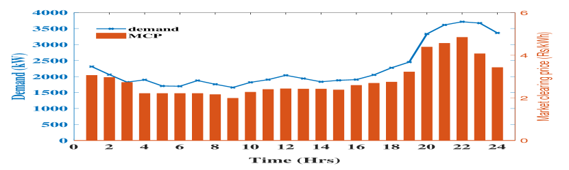
Figure 2: Load demand and MCP considered for the sample day.

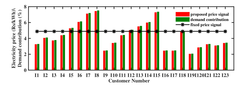
Figure 3: Comparing fixed price and proposed dynamic price considering demand contribution of customers for the given state.

The proposed pricing model is now applied to determine the unit price of all customers for a given state. The analysis is carried for all the system states considering all customers. However, for the ease of analysis the investigation results of industrial customers for the state 22:00 Hr. are presented. The MCP of this state is Rs 4.85. With 1% profit the fixed unit selling price is Rs 4.89. Table I shows the load demand (LD) and unit price (UP) of all the 23 industrial customers, i.e. I1–I23. For this LD, the UP offered to different customers using the proposed dynamic price signal is presented in the table. It can be observed that the UP varies from Rs 2.01 to Rs 7.40, against the fixed price of Rs 4.89. Using MCP and UP the purchase cost of energy and revenue earned by utility are found to be Rs. 5960.12 and Rs. 6019.73, respectively. The profit of the utility is thus Rs 59.60, which is 1% of the purchase cost. If the UP is uniformly kept at Rs 4.89 i.e. fixed price signal generated by MCP for all the customers, the revenue received is found to be Rs. 6019.73 again. This validates that the profit of the utility from the purchase and sale of energy remains unaltered using fixed price or proposed dynamic price signal.

The UP under fixed and proposed dynamic price signals is compared in Fig. 3. It can be observed that the UP using proposed price signal is higher to fixed price only for fewer customers (I5–I8, I12–I15) having demand more than the approximate mean demand of 60 kW. The figure also shows the demand contribution (DC) of all customers. It can be observed that the proposed price signal for each customer is almost proportional to demand contribution of the customer in the peak demand. Therefore, customers with relatively low demand are getting benefited in comparison to flat pricing system. However, the remaining relatively high demand customers have to pay more as per their increased contribution towards peak demand. This shows that the proposed method mitigates the problem of cross-subsidy. Further, from Fig. 4 and Fig. 5, it can be observed that the UP of individual customers belonging to residential and commercial category, respectively, is also changing proportionally on the basis of their contribution in the peak demand.

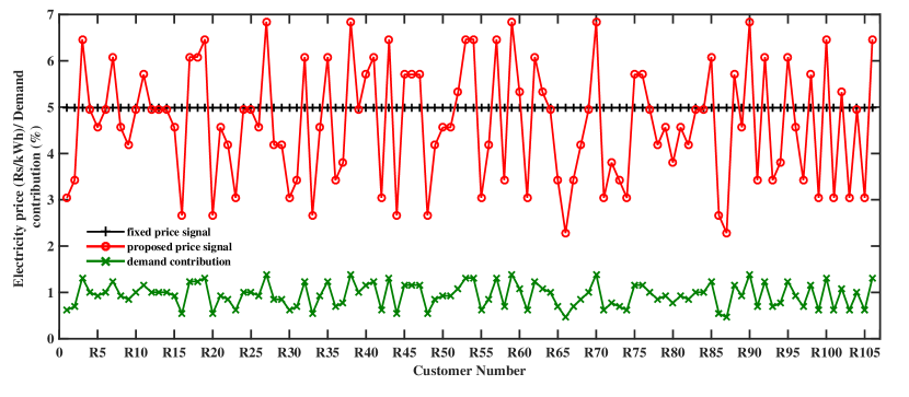
Figure 4: Comparing fixed price and proposed dynamic price considering demand contribution of residential customers for the given state.

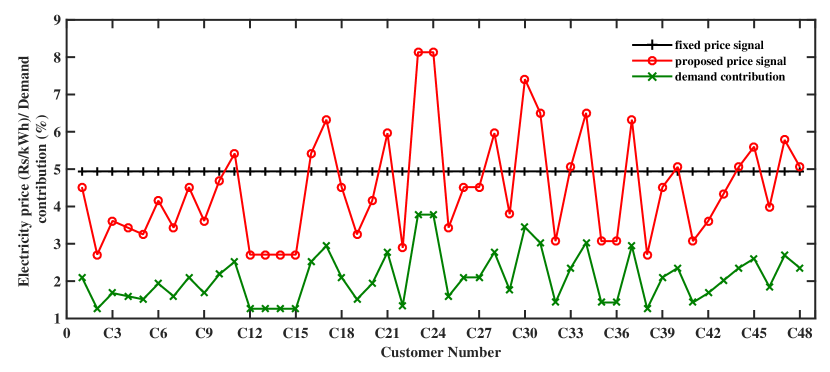
Figure 5: Comparing fixed price and proposed dynamic price considering demand contribution of commercial customers for the given state.

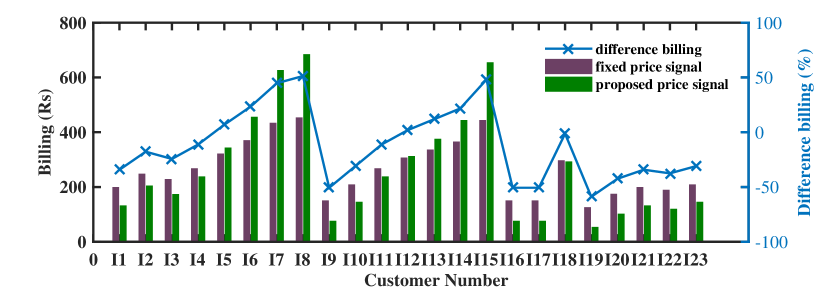
Figure 6: Comparison of billing with fixed price and proposed dynamic price signals for the given state.

The hourly billings of customers with fixed and proposed price signals are compared in Fig. 6. The hourly billing refers to the billing during the given state and will be simply considered as billing throughout the sections IV-A & IV-B. The figure shows that by employing the proposed price signal, the billing depends upon the deviation of demand of customer from the mean demand of the group. The billing is more if the demand is above the mean demand and will be less if it is below the mean demand, and will remain same if the demand is equal to the mean demand. Higher the deviation from the mean demand, more is the variation in billing. The figure shows that low demand customers can have as much as $60\%$ reduced billing whereas high demand customers may have up to $52\%$ increased billing as compared to fixed price signal. The analysis shows that the customers get benefited in billing using proposed dynamic price signal only if their contributions in peak demand are below mean demand of the group, and vice-versa. Thus the proposed pricing system can abolish cross-subsidy without affecting profit of the utility from the sale and purchase of energy. This may greatly relieve the utilities as they do not need to bother about the rebates in billing on the basis of their participation in DRP.

IV-B Detailed Scenario-based Investigation of the Proposed Pricing Model

In order to further validate the robustness of the proposed pricing system, following scenarios are hypothetically considered assuming that the demand of some of the customers would change.

1. Scenario–1 (S1): Demand of two customers is increased by $10\%$

2. Scenario–2 (S2): Demand of two customers is decreased by $10\%$

3. Scenario–3 (S3): Demand of one customer is increased by $10\%$and that of another is decreased by $10\%$

4. Scenario–4 (S4): Non–uniform increase or decrease in demand ($-10\%$ to $+10\%$)

The customer number I8 and I19 have maximum and minimum demand respectively. In order to investigate the effect of proposed pricing model on maximum demand and minimum demand customers, the demand of these customers is only changed in scenarios S1 to S3. The application results of the proposed pricing for scenarios, S1–S3, are summarized in Table II. In the table, the change in load demand ($\Delta$LD) from base value, corresponding change in unit price ($\Delta$UP), change in demand contribution ($\Delta$DC) and change in billing ($\Delta$B) for all the customers are presented. In scenario S1, the customers I8 and I19 have increased their demand by 10%, assuming that the demand of remaining customers remains unchanged. In other words, customers 18 and I19 are not willing to participate in DR. Therefore, these non-willing participants (customers) may be treated as free-riders. The table shows that there is an increase in UP of free-riders by 8.29% with consequent increase in billing by 19.11%. This shows that the free-rider problem can be eliminated using the proposed method as they are suitably penalized in the proposed pricing model. The table also shows evenly reduction in billing of the remaining customers by 1.56%. This marginal reduction may be justified as these customers restrain themselves from increasing their demands.

TABLE II: Results obtained for Scenarios S1, S2 and S3

	S1			S2			S3
	I8	I19	RC	I8	I19	RC	I8	I19	RC
$\triangle$LD (%)	+10	+10	0	-10	-10	0	-10	+10	0
$\triangle$UP (%)	+8.29	+8.29	-1.56	-8.75	-8.75	+1.39	-8.69	+11.60	+1.46
$\triangle$B (%)	+19.11	+19.11	-1.56	-17.88	-17.88	+1.39	-17.82	+22.76	+1.46
$\triangle$DC (%)	+8.96	+8.96	-0.94	-9.13	-9.13	+0.96	-9.51	+10.60	+0.55
PC (Rs)	6016.82			5903.43			5927.66
R (Rs)	6076.99			5962.47			5986.94
P (%)	1.00			1.00			1.00
$\triangle$LD: change in load demand; $\triangle$UP: change in unit price; $\triangle$B: change in billing; RC: remaining customers; PC: purchase cost; R: revenue; P: profit

In scenario S2, the customers I8 and I19 are assumed to decrease their demand by 10%. This shows their pro-active participation in DR. From the table, it may be observed that the UP of these customers has decreased by 9.0%. In this case, the remaining customers become free-riders as they are not actively contributing in DR. Consequently, it may be observed that the UP of these free-riders is increased by 1.39%.

In Scenario S3, the customer I8 decreases demand by 10% and customer I19 increases demand by 10%. This means customer I8 is actively participating in DR whereas customer I19 is a free-rider in existing pricing model who has increased its demand. From the table, it may be observed that the UP of I8 has decreased by 8.69% and that of I19 has increased by 11.60%. The UP of remaining customers has marginally increased due to their indifference towards DRP. This shows that in the proposed pricing model there remains no free-rider.

It can be observed that the penalty imposed in billing to I19 is about 23% in Scenario S3 and the rebate is about 18% in Scenario S2. It happened as $\Delta$DC of I19 is decreased by about 9% in S2, but is increased by about 11% in S3. The table also shows that the profit of the utility remains intact at 1% for all the scenarios (S1–S3). However, the revenue of the utility affects marginally. It happened because the proposed methodology ensures profit of utility as a fixed percentage of purchase cost of energy which depends upon total demand.

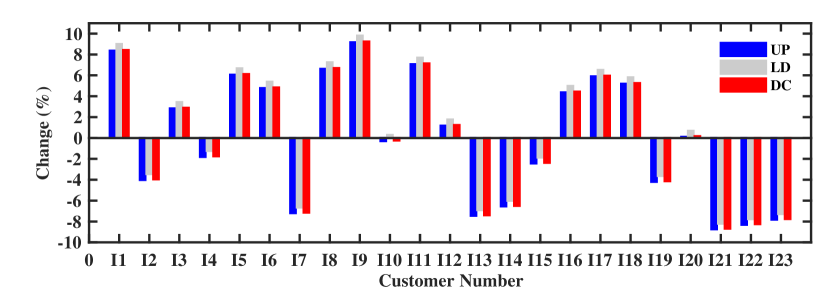
Figure 7: Comparison of change in LD, UP and DC in Scenario S4.

Finally, considering the most practical scenario S4 where the demand of all the customers is assumed to be randomly varied in the range of $\pm 10\%$. The percentage change in LD, UP and DC obtained are presented for comparison in Fig. 7. A general observation can be drawn from the figure that the proposed method causes almost equal change in UP against the change in LD of a customer, and this change in UP is very close to the change in DC of the customer, and the sign of change in LD, UP and DC always remains same. However, very minor exceptions may occur if the magnitude of change in LD is around $1\%$ which is acceptable from practical considerations, as in case of the customers I10 and I20.

TABLE III: Financial comparison of S4 with base case

Particular(s)	Base case	Scenario S4	Difference
Demand (kW)	1230	1236.42	6.42
Purchase cost (Rs)	5960.12	5991.21	31.09
Revenue (Rs)	6019.73	6051.12	31.40
Profit (Rs)	59.60	59.91	0.31

The Table III shows the purchase cost, revenue received and profit incurred to utility in S4 and their comparison with base case. It can be seen from the table that the profit is increased by Rs 0.31 in S4. It happened on account of additional demand of 6.42 kW. The table shows that additional purchase cost is Rs 31.09 for this demand and the corresponding additional revenue received is Rs 31.40. This increases the profit in S4 by Rs 0.31 which is $1\%$ of the additional purchase cost. This is interesting as the sale price of the additional demand of 6.42 kW under the proposed dynamic price signal is unknown, yet the percentage profit remains intact. It implies that the generated price signals adjust themselves for the given profit despite being governed by the individuals’ contribution towards the peak demand.

The above exercise (IV-A & IV-B) and the numerical results obtained so far satisfactorily validates the functionality and data assumptions of the proposed model as expected. After validation of the proposed pricing model with fixed price model, it is extended for comparison with other existing pricing models used in DRPs.

IV-C Comparative Analysis of the Proposed Pricing Model

A comparison of the proposed price signal with the existing price signals like flat, RTP and TOU is performed to analyze and investigate the impact of DR on billing of different categories of customers such as industrial, residential and commercial during peak hours (18:00 Hrs to 23:00 Hrs). For this purpose, MCP profile shown in Fig. 2 is taken as RTP signal while as flat and TOU price signals are generated from this RTP signal in accordance with Ref. [28]. The generated pricing signals like flat, RTP and TOU and load demand profile considered for the 24 hours are shown in Fig. 8 and Fig. 2 respectively. The comparative analysis can also be extended by considering other forms of dynamic price signals like CPP, PTR etc.

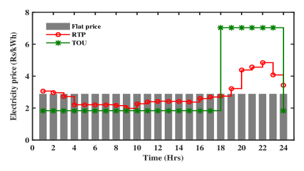
Figure 8: Pricing signals considered for the sample day.

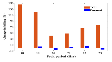
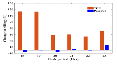
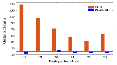
Figure 9: Graphical representation of state-wise percentage change in billing of (a) industrial customers, (b) residential customers and (c) commercial customers during peak hours.

In this section, only economic assessment, in terms of billing of customers, is considered to test the effectiveness of the proposed price signal. The technical assessment is not under the scope of this study. Therefore, the aim of DR here is to shed or curtail the demand in place of shifting. For this analysis, it is assumed that all the categories of customers like residential, commercial and industrial are actively participating in demand response i.e., all the customers are reducing their demand in the range from 0-15% randomly during peak hours. The comparison of collective customer billing over the sample day and during peak hours for all the categories of customers are shown in Table IV and Table V respectively. From the Table IV, it can be observed that the aggregate billing by the proposed price model gives nearly the same results as obtained by RTP price model. It is important to recall that RTP is based on MCP and that is why it is considered to be most accurate. It may also be observed from the table that aggregate billing obtained by flat rate price signal is appreciably less than RTP which is a loss to the utility. On the other hand, the aggregate billing obtained by TOU pricing signal is much higher than that obtained by RTP. The higher billing offered by TOU is a loss to the customers and therefore it will have lesser acceptability to the customers. These results verify that the proposed price model despite mitigating cross-subsidy and free-rider problems does not affect overall billing in terms of revenue. The comparison of collective customer billing during peak hours for all the categories of customers are shown in Table V. From the table, it may be observed that TOU price model is charging exorbitantly higher from the customer during peak hours as compared to RTP pricing model. This exorbitantly higher billing has no justification. However, the proposed price model gives nearly the same results as obtained by RTP pricing model.

TABLE IV: Comparison of aggregate billing over the 24 hours

Price signal	Billing (Rs)			Total (Rs)
	Industrial customers	Residential customers	Commercial customers
Flat	51667.58	54397.98	49987.34	156052.9
RTP	54395.74	58713.36	53720.32	166829.4
TOU	63171.28	66365.98	60928.84	190466.1
Proposed	54425.49	59383.41	52962.47	166771.4

TABLE V: Comparison of aggregate billing over the peak hours

Price signal	Billing (Rs)			Total (Rs)
	Industrial customers	Residential customers	Commercial customers
Flat	18041.93	18995.37	17455.2	54492.50
RTP	24180.33	26271.26	24198.09	74649.68
TOU	41400.83	42991.18	39657.83	124049.84
Proposed	24210.08	26941.31	23440.25	74591.64

TABLE VI: Comparison of state-wise billing of all the customers over the peak hours

Customer category	Price signal	Billing (Rs)
		Peak hours
		18	19	20	21	22	23
Industrial customers	Flat	2153.09	2321.20	3154.46	3421.92	3515.67	3475.61
	RTP	1929.75	2380.41	4816.69	4995.68	5217.18	4840.63
	TOU	4741.07	5251.57	6775.33	7395.10	8659.09	8578.68
	Proposed	1924.63	2488.36	4523.20	5117.46	5572.54	4583.90
Residential customers	Flat	2266.87	2443.86	3321.16	3602.76	3701.45	3659.28
	RTP	2197.67	2618.22	5128.18	5221.79	6029.29	5076.13
	TOU	4909.78	5834.38	7610.34	7827.19	8660.66	8148.84
	Proposed	2084.19	2610.09	4857.19	5445.94	5993.89	5950.01
Commercial customers	Flat	2083.07	2245.71	3051.88	3310.64	3401.33	3362.58
	RTP	2022.23	2372.34	4233.49	5200.21	5669.29	4700.53
	TOU	5025.88	4879.22	7291.99	7638.25	7526.04	7296.46
	Proposed	1877.38	2368.11	4391.65	4950.39	5353.95	4498.77

The Table VI shows the state-wise comparison of customer billing during peak hours. The percentage change in billing of industrial, residential and commercial customers with reference to the RTP signal during peak hours is shown in Fig. 9(a)–9(c). In these figures, the change in billing below horizontal axis indicates percentage reduction in billing while as the change in billing above horizontal axis denotes percentage increase in billing of customers. Among existing dynamic pricing signals, RTP signal is known to offer potentially highest reward but with more risk. On the Contrary, the TOU signal offers the least potential reward at the lowest risk [1, 44, 18]. However, from Fig. 9(a)–9(c) it can be observed that the proposed price signal can offer more reward (in terms of bill savings) most of the times as compared to RTP signal with lowest risk as it remains static during off-peak hours just like TOU price signal. The proposed price model shows gradual enhancement in reward when moving from high consumption to low consumption customers. This can bring a sense of motivation and eagerness in low consumption customers (which are usually low income customers) to actively participate in DRPs unlike existing price models. Also, it is interesting to note that the proposed price signal offers lowest billing for customers during 18:00 Hrs in all the three categories, which is evident from Fig. 9(a)–9(c). Therefore, the proposed price signal is best suitable, promising, least-risky and economically efficient for both the risk-averse as well as risk-taking customers among the dynamic pricing options.

V Conclusion

A demand contribution based dynamic price model is presented for successful implementation of PBDR in the distribution systems. The price signal is designed in such a way that the unit price varies proportionately with the individual’s concurrent demand during on-peak hours, but remains static otherwise. The proposed price model is class apart than other existing counterparts as it imposes different dynamic price signals to different customers during the same time period.

The proposed dynamic price model has been thoroughly investigated on benchmark 33-bus test distribution system under different operating scenario. The application results obtained are also compared with existing dynamic pricing models. The simulation results reveal that the proposed price model varies billing of customers in accordance to the change in their demand. Detailed investigation of the obtained results reveals that the proposed model can overcome chronic problems of DRPs such as cross-subsidy and free-riders while the customers get fair and transparent allocation of financial benefits. The proposed dynamic pricing model suitably rewards the customers who are actively participating and penalizes the customers who do not actively participate in dynamic pricing programs due to their financial flexibility. The comparative analysis shows that the proposed price signal can offer more reward, in terms of bill savings, as compared to other dynamic price signals with lowest risk. The analysis shows gradual enhancement in procuring reward by the customers when moving from high consumption to low consumption customers. This can bring a sense of motivation and interest in low consumption customers to actively participate in DRPs unlike existing dynamic price models. In addition, the proposed model not only preserves assured profit of the utilities but also fully relieved them to deliver financial benefits of DR to the participating customers. The chances of rebound effect may be less using the developed model because it imposes diverse price differentials among the customers. Moreover, the major chunk of the customers gets benefited in electricity billing thus enhances fair chances in DR participation. Proposed model attempts to provide win-win situation to both the customers and the utility. The model is quite unique and innovative, however, may lack public acceptance initially unless supported by intense DR education programs, as in existing models. It is highly simplified, straight forward, and effective but requires advanced ICT infrastructure for implementation. The proposed price model preserves assured percentage profit of utility. The present work can also be used for emergency demand response programs.

Appendix

The detail of the customers’ loading is given in Table A-1.

TABLE A-1: Hourly load data assumed for the individual customers of the system under study

CT	LD	CT	LD	CT	LD	CT	LD	CT	LD	CT	LD	CT	LD	CT	LD
R1	8	R24	13	R46	15	R68	11	R90	18	C6	23	C28	33	I2	50
R2	9	R25	13	R47	15	R69	13	R91	9	C7	19	C29	21	I3	46
R3	17	R26	12	R48	7	R70	18	R92	16	C8	25	C30	41	I4	54
R4	13	R27	18	R49	11	R71	8	R93	9	C9	20	C31	36	I5	65
R5	12	R28	11	R50	12	R72	10	R94	10	C10	26	C32	17	I6	75
R6	13	R29	11	R51	12	R73	9	R95	16	C11	30	C33	28	I7	88
R7	16	R30	8	R52	14	R74	8	R96	12	C12	15	C34	36	I8	92
R8	12	R31	9	R53	17	R75	15	R97	9	C13	15	C35	17	I9	30
R9	11	R32	16	R54	17	R76	15	R98	15	C14	15	C36	17	I10	42
R10	13	R33	7	R55	8	R77	13	R99	8	C15	15	C37	35	I11	54
R11	15	R34	12	R56	11	R78	11	R100	17	C16	30	C38	15	I12	62
R12	13	R35	16	R57	17	R79	12	R101	8	C17	35	C39	25	I13	68
R13	13	R36	9	R58	9	R80	10	R102	14	C18	25	C40	28	I14	74
R14	13	R37	10	R59	18	R81	12	R103	8	C19	18	C41	17	I15	90
R15	12	R38	18	R60	14	R82	11	R104	13	C20	23	C42	20	I16	30
R16	7	R39	13	R61	8	R83	13	R105	8	C21	33	C43	24	I17	30
R17	16	R40	15	R62	16	R84	13	R106	17	C22	16	C44	28	I18	60
R18	16	R41	16	R63	14	R85	16	C1	25	C23	45	C45	31	I19	25
R19	17	R42	8	R64	13	R86	7	C2	15	C24	45	C46	22	I20	35
R20	7	R43	17	R65	9	R87	6	C3	20	C25	19	C47	32	I21	40
R21	12	R44	7	R66	6	R88	15	C4	19	C26	25	C48	28	I22	38
R22	11	R45	15	R67	9	R89	12	C5	18	C27	25	I1	40	I23	42
R23	8
CT: customer type (R: residential, C: commercial, I: industrial); LD: load demand

References

- [1] A. Faruqui, S. Sergici, and J. Palmer, “The impact of dynamic pricing on low income customers,” Institute for Electric Efficiency Whitepaper, 2010.
- [2] D. S. Kirschen, “Demand-side view of electricity markets,” IEEE Transactions on Power Systems, vol. 18, no. 2, pp. 520–527, May 2003.
- [3] U. DoE, “Benefits of demand response in electricity markets and recommendations for achieving them. a report to the united states congress pursuant to section 1252 of the energy policy act of 2005,” in US Washington, DC: Department of Energy.[http://eetd. lbl. gov/ea/EMP/reports/congress-1252d. pdf](26 July 2009), 2006.
- [4] F. Staff, “Assessment of demand response and advanced metering,” Federal Energy Regulatory Commission, Docket AD-06-2-000, 2006.
- [5] F. E. R. Commission et al., “Staff report-assessment of demand response and advanced metering,” 2007.
- [6] U. F. E. R. Commission et al., “A national assessment of demand response potential,” Staff Report, Washington, DC. p, Tech. Rep., 2009.
- [7] C.-J. Yang, “Opportunities and barriers to demand response in china,” Resources, Conservation and Recycling, vol. 121, pp. 51–55, 2017.
- [8] C. Goldman, M. Reid, R. Levy, and A. Silverstein, “Coordination of energy efficiency and demand response,” 06 2010.
- [9] C. Ahn, C.-T. Li, and H. Peng, “Optimal decentralized charging control algorithm for electrified vehicles connected to smart grid,” Journal of Power Sources, vol. 196, no. 23, pp. 10 369–10 379, 2011.
- [10] D. Kirschen and G. Strbac, “Fundamentals of power system economics: Copyright© 2004 john wiley & sons,” 2005.
- [11] M. Hussain and Y. Gao, “A review of demand response in an efficient smart grid environment,” The Electricity Journal, vol. 31, no. 5, pp. 55–63, 2018.
- [12] Q. Zhang and J. Li, “Demand response in electricity markets: A review,” in 2012 9th International Conference on the European Energy Market, May 2012, pp. 1–8.
- [13] M. A. F. Ghazvini, J. Soares, O. Abrishambaf, R. Castro, and Z. Vale, “Demand response implementation in smart households,” Energy and buildings, vol. 143, pp. 129–148, 2017.
- [14] P. Palensky and D. Dietrich, “Demand side management: Demand response, intelligent energy systems, and smart loads,” IEEE transactions on industrial informatics, vol. 7, no. 3, pp. 381–388, 2011.
- [15] B. Daryanian, R. E. Bohn, and R. D. Tabors, “Optimal demand-side response to electricity spot prices for storage-type customers,” IEEE Transactions on Power Systems, vol. 4, no. 3, pp. 897–903, Aug 1989.
- [16] J. G. Roos and I. E. Lane, “Industrial power demand response analysis for one-part real-time pricing,” IEEE Transactions on Power Systems, vol. 13, no. 1, pp. 159–164, Feb 1998.
- [17] P. M. Schwarz, T. N. Taylor, M. Birmingham, and S. L. Dardan, “Industrial response to electricity real-time prices: Short run and long run,” Economic Inquiry, vol. 40, no. 4, pp. 597–610, 2002.
- [18] A. Faruqui, R. Hledik, and J. Palmer, Time-varying and dynamic rate design. Regulatory Assistance Project, 2012.
- [19] J. T. Wenders, “Peak load pricing in the electric utility industry,” The Bell Journal of Economics, pp. 232–241, 1976.
- [20] J.-N. Sheen, C.-S. Chen, and T.-Y. Wang, “Response of large industrial customers to electricity pricing by voluntary time-of-use in taiwan,” IEE Proceedings-Generation, Transmission and Distribution, vol. 142, no. 2, pp. 157–166, 1995.
- [21] N. Yu and J.-l. Yu, “Optimal tou decision considering demand response model,” in 2006 International Conference on Power System Technology. IEEE, 2006, pp. 1–5.
- [22] A. David and Y. Li, “Effect of inter-temporal factors on the real time pricing of electricity,” IEEE transactions on power systems, vol. 8, no. 1, pp. 44–52, 1993.
- [23] D. S. Kirschen, G. Strbac, P. Cumperayot, and D. de Paiva Mendes, “Factoring the elasticity of demand in electricity prices,” IEEE Transactions on Power Systems, vol. 15, no. 2, pp. 612–617, 2000.
- [24] E. Celebi and J. D. Fuller, “A model for efficient consumer pricing schemes in electricity markets,” IEEE Transactions on Power Systems, vol. 22, no. 1, pp. 60–67, 2007.
- [25] J.-N. Sheen, C.-S. Chen, and J.-K. Yang, “Time-of-use pricing for load management programs in taiwan power company,” IEEE Transactions on Power Systems, vol. 9, no. 1, pp. 388–396, 1994.
- [26] H. Aalami, G. Yousefi, and M. P. Moghadam, “Demand response model considering edrp and tou programs,” in 2008 IEEE/PES Transmission and Distribution Conference and Exposition. IEEE, 2008, pp. 1–6.
- [27] D. Duan, J. Liu, H. Niu, and J. Wu, “A risk-evasion tou pricing method for distribution utility in deregulated market environment,” in 2004 International Conference on Power System Technology, 2004. PowerCon 2004., vol. 1. IEEE, 2004, pp. 527–531.
- [28] A. Faruqui, “Chapter 3 - the ethics of dynamic pricing,” in Smart Grid, F. P. Sioshansi, Ed. Boston: Academic Press, 2012, pp. 61 – 83. [Online]. Available: http://www.sciencedirect.com/science/article/pii/B9780123864529000036
- [29] D. T. Nguyen, M. Negnevitsky, and M. de Groot, “Pool-based demand response exchange—concept and modeling,” IEEE Transactions on Power Systems, vol. 26, no. 3, pp. 1677–1685, Aug 2011.
- [30] W. Zhang, K. Kalsi, J. Fuller, M. Elizondo, and D. Chassin, “Aggregate model for heterogeneous thermostatically controlled loads with demand response,” in 2012 IEEE Power and Energy Society General Meeting, July 2012, pp. 1–8.
- [31] H. Bitaraf and S. Rahman, “Reducing curtailed wind energy through energy storage and demand response,” IEEE Transactions on Sustainable Energy, vol. 9, no. 1, pp. 228–236, Jan 2018.
- [32] H. Allcott, “Rethinking real-time electricity pricing,” Resource and energy economics, vol. 33, no. 4, pp. 820–842, 2011.
- [33] T. Ericson, “Direct load control of residential water heaters,” Energy Policy, vol. 37, no. 9, pp. 3502–3512, 2009.
- [34] S. Berg, “Basics of rate design: Pricing principles and self-selecting two-part tariffs,” Infrastructure regulation and market reform: Principles and practice, pp. 74–90, 1998.
- [35] B. Lin and X. Liu, “Electricity tariff reform and rebound effect of residential electricity consumption in china,” Energy, vol. 59, pp. 240–247, 2013.
- [36] E. Cutter, C. K. Woo, F. Kahrl, and A. Taylor, “Maximizing the value of responsive load,” The Electricity Journal, vol. 25, no. 7, pp. 6–16, 2012.
- [37] A. Star, M. Isaacson, D. Haeg, L. Kotewa, and C. Energy, “The dynamic pricing mousetrap: Why isn’t the world beating down our door,” in ACEEE summer study on energy efficiency in buildings, 2010, pp. 257–268.
- [38] C. Su and D. Kirschen, “Quantifying the effect of demand response on electricity markets,” IEEE Transactions on Power Systems, vol. 24, no. 3, pp. 1199–1207, Aug 2009.
- [39] E. R. Brubaker, “Free ride, free revelation, or golden rule?” The Journal of Law and Economics, vol. 18, no. 1, pp. 147–161, 1975.
- [40] M. Bagnoli and B. L. Lipman, “Provision of public goods: Fully implementing the core through private contributions,” The Review of Economic Studies, vol. 56, no. 4, pp. 583–601, 1989.
- [41] M. E. Baran and F. F. Wu, “Network reconfiguration in distribution systems for loss reduction and load balancing,” IEEE Power Engineering Review, vol. 9, no. 4, pp. 101–102, 1989.
- [42] Indian Energy Exchange [Online] Available: https://www.iexindia.com/.
- [43] N. Kanwar, N. Gupta, K. R. Niazi, and A. Swarnkar, “Optimal distributed resource planning for microgrids under uncertain environment,” IET Renewable Power Generation, vol. 12, no. 2, pp. 244–251, 2018.
- [44] A. Faruqui and J. Palmer, “Dynamic pricing and its discontents,” Regulation, vol. 34, p. 16, 2011.