Optimal collision avoidance in swarms of active Brownian particles

Abstract

The effectiveness of collective navigation of biological or artificial agents requires to accommodate for contrasting requirements, such as staying in a group while avoiding close encounters and at the same time limiting the energy expenditure for manoeuvring. Here, we address this problem by considering a system of active Brownian particles in a finite two-dimensional domain and ask what is the control that realizes the optimal tradeoff between collision avoidance and control expenditure. We couch this problem in the language of optimal stochastic control theory and by means of a mean-field game approach we derive an analytic mean-field solution, characterized by a second-order phase transition in the alignment order parameter. We find that a mean-field version of a classical model for collective motion based on alignment interactions (Vicsek model) performs remarkably close to the optimal control. Our results substantiate the view that observed group behaviors may be explained as the result of optimizing multiple objectives and offer a theoretical ground for biomimetic algorithms used for artificial agents.

1 Introduction

Awe-inspiring examples of organized collective motions abound in a number of biological problems [1, 2] from simple microorganisms such as bacteria [3], to insects and higher animals which display deliberate social behaviors such as insect swarming [4, 5] bird flocking [6, 7], and fish schooling or shoaling [8, 9]. Most impressively, large and dense groups of animals can organize themselves in complex coordinated motions avoiding collisions while flying or swimming at close distance. Several models have been proposed to model the origin of such phenomena in terms of simple behavioral rules. A first intuition of the basic ingredients came from computer graphics [10] and entered the domain of statistical physics with the Vicsek model [11]: the core idea is that each animal in the group needs to align its heading direction with the mean direction of its neighbors. If such local alignment interactions are strong enough with respect to the unavoidable noise (in our case, on the heading directions) a transition from a disordered phase to a collective-order phase, characterized by global orientational order (alignment) of the heading directions, may occur. This idea was also applied, for instance, to the control of groups of artificial agents such as robots, where collision avoidance is crucial [12, 13]. Overall, these approaches generally build agent-based models aimed at generating certain collective behaviors starting from intuition, observations or by reverse-engineering natural phenomena via data analysis; this often leads to biomimetic algorithms for robotics.

In this paper, we try to approach the problem of collision avoidance from a different perspective. We do not aim at modeling the interactions that underlie a certain collective behavior, but instead we consider a simple model of swarming agents and explicitly set the goal of avoiding collisions in the form a cost function and ask the following questions: What is the optimal choice of control which minimizes the collective cost? How does the optimal control compare with known agent-based models which lead to collision avoidance?

The natural setting to answer the above questions is that of optimal control theory [14] and mean-field game formalism [15, 16]. Similar approaches, indeed, have already been shown to yield promising results. For instance, for collective search problems the optimal control reduces in some limit to a well known model of chemotaxis [17], for the problem swarming agents in one-dimensional disordered environments [18], and also for flocking problems with the aid of reinforcement learning techniques [19].

In what follows, we start by introducing the setting of the problem in Sec. 2.1 where also the optimal control formalism is presented. We model agents as active Brownian particles [20, 21] which move in two-dimensions and whose heading direction is subject to rotational noise. They try to avoid collisions by exerting some control on their heading direction, in the form of a torque. Collisions lead to a cost, but also the control itself is not free of charge, and for that we assume a quadratic dependence in the angular velocity. The cost for control can either be understood in terms of power dissipation, physical limitations of an animal/robot, or in terms of the cognitive cost of deviating from free spontaneous behavior [14]. Therefore, an agent is interested in applying a non-trivial control to its motion only to the extent to which the gain outweighs the cost: the optimal strategy emerges from this tradeoff. This cost minimization problem can be exactly mapped into a quantum many-body problem which is unfortunately hard to solve in general. For this reason, we introduce a mean field approximation (Sec. 2.2) that reduces the many-body problem to a quantum pendulum, which is exactly solvable. Under this approximations, agents are assumed to be homogeneously distributed. While this is unrealistic under many respects, it can suitably describe the optimal behavior over an approximately uniform region in the bulk of a swarm. We show that all relevant parameters combine into a fundamental tradeoff parameter $h$, which effectively accounts for the balance between the collision and control costs. Upon increasing such tradeoff parameter, the system displays a second order phase transition in terms of the polar order parameter (a measure of the mean-field alignment) at a certain critical value $h_{c}$. Then, we study some relevant observables, such as the cost, the polar order and the susceptivity – which is known to be important in collective motions [22] – both near the critical point (Sec. 2.3) and in the strong coupling regime (large $h$, corresponding to collisions costs dominating, see Sec. 2.4).

Remarkably, in both limits, the optimal control is well approximated by a sinusoidal function of the difference between the individual heading direction (angle) and the mean one (Sec. 3.1). Interestingly, the sinusoidal control is a distinctive trait of the well-known Vicsek-like models [2, 23, 24] and its mean-field versions [25, 26, 27]. This observation motivates a vis à vis comparison between the optimal and sinusoidal control. For a sound comparison, we first find the sinusoidal control which minimizes the total cost (Sec. 3.2). Remarkably, such best sinusoidal model is controlled by the same tradeoff parameter, and the polar order turns out to display a second order transition at the same critical point as for the optimal model; with analytical tools, we explore this regime along with the strong coupling one. Finally, we proceed with a systematic comparison (Sec. 3.3) in the whole range of the tradeoff parameter, showing how the optimal solution, while close to its sinusoidal approximation, can better manage the collisions, and that the sinusoidal model becomes the exact optimum in the strong coupling (large $h$) limit. The last section is dedicated to discussion and outlook (Sec. 4). Some derivations and technical material are moved to the Appendices.

2 Optimal solution of the collision problem

2.1 Collision minimization as an optimal control problem

We consider a group of $N$ agents in two dimensions whose goal is to swarm together while avoiding collisions with each other (see Fig. 1). We model the agents as active Brownian particles [20, 21]: each agent $i$ is a self-propelled particle moving with a constant speed $u_{0}$ in a direction identified by an angle $\theta_{i}$ (or, equivalently, by the associated unitary vector $\bm{n}(\theta_{i})=(\cos\theta_{i},\sin\theta_{i})$) which randomly changes due to rotational noise with diffusivity $D$. Each agent, to avoid collisions, can exert some control, $f_{i}$, on its angular velocity and possibly contrast the rotational noise. The controls $f_{i}$ are, in the most general case, functions of all positions, $\bm{x}_{j}$, and heading directions, $\theta_{j}$, of all agents ($j=1,\ldots,N$). The dynamics of agent $i$ thus reads

$$\begin{dcases}d\bm{x}_{i}=u_{0}\,\bm{n}(\theta_{i})dt\\ d\theta_{i}=f_{i}(\bm{x}_{i},\theta_{i};\{\bm{x}_{j},\theta_{j}\}_{j\neq i})\,dt+\sqrt{2\,D}\,d\xi_{i}\,,\end{dcases}$$ (1)

where the noise term in the angular dynamics is a zero mean, $\langle d\xi_{i}(t)\rangle=0$, Gaussian process with correlation $\langle d\xi_{i}(t)\;d\xi_{j}(t^{\prime})\rangle=\delta_{ij}\,\delta(t-t^{\prime})\;dt$. We assume periodic boundary conditions, since we are only interested in the bulk interactions within the swarm. This choice will not be relevant for the rest of the paper.

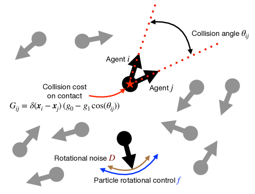
Figure 1: Sketch of the swarming active Brownian particles. The black particle on the bottom illustrates the angular dynamics influenced by rotational noise (brown arrows) and the control (blue arrows). The couple of black particles on the top, denoted $i$ and $j$, illustrates the cost paid for each contact, depending on the collision angle. The agents can avoid the collisions by controlling their angular velocity, but pay a cost for it.

When particle pairs, say $i$ and $j$, collide they pay a cost $G_{ij}=\delta(\bm{x}_{i}-\bm{x}_{j})\,\mathcal{G}(\theta_{ij})$ with $\mathcal{G}(\theta_{ij})$ representing the functional dependence of cost on the collision angle, $\theta_{ij}=(\theta_{i}-\theta_{j})$. By expanding $\mathcal{G}(\theta)=g_{0}+g_{1}\cos\theta+g_{2}\cos(2\theta)+...$ into (even) harmonics and truncating after the second term, we obtain $G_{ij}=\delta(\bm{x}_{i}-\bm{x}_{j})\,(g_{0}-g_{1}\,\bm{n}(\theta_{i})\cdot\bm{n}(\theta_{j}))=\delta(\bm{x}_{i}-\bm{x}_{j})\,(g_{0}-g_{1}\cos\theta_{ij})$. As we will see, the cost per contact $g_{0}>0$ will be somehow unimportant but its relationship with angular cost $g_{1}>0$ allows for different model interpretations. For instance, if $g_{0}=0$ we have a pure alignment problem, while for $g_{1}=g_{0}$ we have a pure collision-based model, as in the latter case the collision cost is proportional to the relative velocity which is exactly zero when velocities are aligned.

Agent $i$ can partially control its heading direction by imparting an angular velocity $f_{i}$ but it pays a cost $\alpha\,f_{i}^{2}/2$. The quadratic choice for the cost of control, besides being quite natural when interpreted in terms of power dissipation, has an information-theoretical foundation as the cost (measured in terms of the Kullback-Leibler divergence) of deviating from a random control strategy [14]. The total cost per unit time - the sum of individual costs - reads

$$C(\bm{x}_{1},\theta_{1};...;\bm{x}_{N},\theta_{N})=\frac{\alpha}{2}\sum_{i}f_{i}^{2}+\frac{1}{2}\sum_{i\neq j}\delta(\bm{x}_{i}-\bm{x}_{j})\,(g_{0}-g_{1}\,\bm{n}(\theta_{i})\cdot\bm{n}(\theta_{j}))\,.$$ (2)

Notice that the parameter $\alpha>0$ can be reabsorbed in the definition of $g_{0}$ and $g_{1}$, since we are only interested in the optimal strategy, while it would have played a role in risk-sensitive scenarios [17, 28, 29].

The agents collective goal is to choose the controls that minimize the average total cost $\bar{C}=\int\prod_{k=1}^{N}d\bm{x}_{k}\,d\theta_{k}\;C(\bm{x}_{1},\theta_{1};...;\bm{x}_{N},\theta_{N})\;P(\bm{x}_{1},\theta_{1};...;\bm{x}_{N},\theta_{N})$, with $P$ being the stationary joint probability density of particles positions and angles. The non-trivial point is that $P$ itself depends on the controls $\{f_{i}\}_{i=1}^{N}$ and should be determined as part of the solution. In particular, the joint probability $P$, besides the normalization constraint $\int\prod_{k=1}^{N}d\bm{x}_{k}\,d\theta_{k}\;P(\bm{x}_{1},\theta_{1};...;\bm{x}_{N},\theta_{N})=1$, must be the stationary solution of the Fokker-Planck equation associated to Eq. (1), which reads

$$\sum_{i=1}^{N}\left[-u_{0}\,\partial_{\bm{x}_{i}}\;\bm{n}(\theta_{i})-\sum_{i}\partial_{\theta_{i}}\;f_{i}+D\;\sum_{i}\partial^{2}_{\theta_{i}}\right]P=\sum_{i=1}^{N}\mathcal{L}_{i}\,P=\mathcal{L}_{(N)}P=0\,,$$ (3)

where $\mathcal{L}_{i}$ is the single-agent linear Fokker-Planck operator and $\mathcal{L}_{(N)}=\sum_{i}\mathcal{L}_{i}$ the $N$-bodies one. By minimizing the total cost, we are looking for a cooperative solution to the problem. The solution of the constrained minimization can obtained by a generalized Lagrange-multipliers technique, or namely, by finding the stationary points of the auxiliary functional (Pontryagin principle [30])

$$\mathcal{H}=\lambda+\int\prod_{i=1}^{N}d\bm{x}_{i}\,d\theta_{i}\;\,[C-\lambda-\Phi\,\mathcal{L}_{N}]\,P\,.$$ (4)

The normalization and dynamical constraints are obtained by imposing stationarity w.r.t. (with respect to) the multipliers $\lambda$ and $\Phi(\bm{x}_{1},\theta_{1};...;\bm{x}_{N},\theta_{N})$, respectively. The non-trivial results come from the request of stationarity w.r.t. $P$ and $f_{i}$, which yields

$$\frac{\delta\mathcal{H}}{\delta f_{i}}=0\implies f_{i}=\partial_{\theta_{i}}\Phi$$ (5)

$$\frac{\delta\mathcal{H}}{\delta P}=0\implies C-\lambda-u_{0}\,\sum_{i}\bm{n}(\theta_{i})\cdot\partial_{\bm{x}_{i}}\;\Phi-\sum_{i}f_{i}\,\partial_{\theta_{i}}\;\Phi-D\;\sum_{i}\partial^{2}_{\theta_{i}}\Phi=0\,.$$ (6)

Equation (6) is the Hamilton-Jacobi-Bellman equation associated to the optimal control problem. It can be linearized via the Hopf–Cole transform, $\Phi\!=\!2D\,\log Z$, by introducing the desirability function $Z(\bm{x}_{1},\theta_{1};...;\bm{x}_{N},\theta_{N})$ [14]. Then the control (5) becomes

$$f_{i}=2\,D\,\partial_{\theta_{i}}\ln Z\,,$$ (7)

that is a gradient ascent towards more desirable configurations, hence the name. Thanks to the Hopf–Cole transform, Eq. (6) becomes the linearized Bellman equation

$$\frac{\lambda}{2\,D}\,Z-\frac{1}{4D}\sum_{i\neq j}\delta(\bm{x}_{i}-\bm{x}_{j})\,(g_{0}-g_{1}\,\bm{n}(\theta_{i})\cdot\bm{n}(\theta_{j}))\,Z+u_{0}\,\sum_{i}\bm{n}(\theta_{i})\cdot\partial_{\bm{x}_{i}}\;Z+D\;\sum_{i}\partial^{2}_{\theta_{i}}\,Z=0\,.$$ (8)

which is formally identical to the stationary Schrödinger equation of $N$ identical, interacting bosons. We should solve both for the ground-state eigenvalue $\lambda/2D$, which can be shown to be proportional to the total cost, and the eigenfunction $Z$, requiring $Z$ to be real and positive. To our knowledge, this quantum many-body problem has no known general solution for generic $N$; therefore, we will seek for the optimal control in an approximate mean field setting.

2.2 Mean field approximation

To simplify the problem and make it exactly solvable, we proceed with a mean field approximation based on two hypothesis: first we assume agent-wise factorization of the desirability $Z$ and then we assume spatial homogeneity - no preferred points in space, only preferred directions. The agent-wise factorization excludes direct pairwise interactions – agents cannot directly dodge each other – but, rather, each agent interacts with the joint probability of the remaining $N-1$ ones in a self consistent manner. This approximation is rather strong since in animal collective behavior it would make more sense to consider local interactions [6]. It must also be remarked that the homogeneity assumption excludes from the description many interesting phenomena related to heterogeneities. Notwithstanding these limitations, we can still assume that this treatment could be relevant to describe agents within a uniform bulk region of the swarm.

With the factorization and homogeneity assumptions, the desirability can be written as

$$Z(\bm{x}_{1},\theta_{1},...,\bm{x}_{N},\theta_{N})=\prod_{i=1}^{N}\zeta(\theta_{i})\,,$$ (9)

and, equivalently $\Phi(\bm{x}_{1},\theta_{1},...,\bm{x}_{N},\theta_{N})=\sum_{i=1}^{N}\phi(\theta_{i})$. As a consequence, the probability $P$ is factorized as $P(\bm{x}_{1},\theta_{1},...,\bm{x}_{N},\theta_{N})=\prod_{i=1}^{N}p(\bm{x}_{i},\theta_{i})$ and, owing to spatial homogeneity, we can write $p(\bm{x}_{i},\theta_{i})=\frac{1}{V}\rho(\theta_{i})$, with $V$ being the area where the swarm moves.

We define the agents’ average heading direction $\bar{\theta}$ and the polar order parameter (alignment parameter or polarization) $m$ as

$$m\,\bm{n}(\bar{\theta})=\int d\theta^{\prime}\;\bm{n}(\theta^{\prime})\,\rho(\theta^{\prime})\,,$$ (10)

in terms of which the average agent speed reads $\langle\dot{\bm{x}}\rangle=m\,u_{0}\,\bm{n}(\bar{\theta})$; here and in the sequel, since all particles are equivalent by mean-field ansatz, we drop particle indices.

By defining the parameter $\delta=(N-1)/V$, which is the particle density measured by a reference agent, and $C_{0}=\delta\,g_{0}/2$, with a few straightforward passages, we write the average per agent cost as

$$\bar{C}=C_{0}+\int d\theta\;\rho(\theta)\;\left[-\frac{\delta\,m\,g_{1}}{2}\;\cos(\theta-\bar{\theta})+\frac{1}{2}f^{2}\right]\,,$$ (11)

and the functional (4) as

$$\mathcal{H}=\lambda+\bar{C}-\int d\theta\;[\lambda+\phi(\theta)\;\mathcal{L}\,]\rho(\theta)\,,$$ (12)

with $\mathcal{L}=-\partial_{\theta}f+D\,\partial_{\theta}^{2}$ being the single-particle Fokker-Planck operator as in Eq. (3). Proceeding analogously to the general case and by exploiting the Hopf-Cole transform with the factorized desirability (9), we derive the control to be

$$f(\theta)=2\,D\,\frac{d}{d\theta}\ln\zeta\,.$$ (13)

Plugging the last expression into the stationary Fokker-Planck equation, $\mathcal{L}\,\rho=0$, with periodic boundary conditions, yields

$$\rho=\zeta^{2}\,,$$ (14)

with $\int d\theta\;\zeta^{2}=1$. Therefore, the optimal control problem boils down to solving the self-consistent system of equations

$$m=\int d\theta\;\cos\theta\;\zeta^{2}$$ (15)

$$\left[\frac{\lambda}{2D}+\frac{\delta\,m\,g_{1}}{2D}\;\cos\theta\right]\,\zeta+D\,\partial_{\theta}^{2}\zeta=0\,.$$ (16)

Equation (15) is just Eq. (10) where we used (14) and fixed $\bar{\theta}=0$ with no loss of generality, as the rotational symmetry can be broken in an arbitrary direction, while Eq. (16) is the mean-field linearized Bellman equation with $\bar{\theta}=0$. Formally, Eq. (16) is the stationary Schrödinger equation for a quantum pendulum also known as Mathieu equation that, for consistency with literature [31, 32], we rewrite in the canonical form

$$\left[a-2\,q\,\cos(2\,y)\right]\,\zeta+\zeta^{\prime\prime}=0.$$ (17)

with $y\!=\!\theta/2$, $a\!=\!-\!\lambda/(2\,D^{2})$, $q\!=\!-\!\delta\,m\,g_{1}/D^{2}$, and ^′′ denoting the second derivative with respect to $y$. Equation (17) must be solved both for the eigenvalue $-a$ (which corresponds to solving for $\lambda$) and the eigenfunction $\zeta\!=\!\zeta_{m}$, which depends parametrically on $m$. The solutions are the so-called Mathieu functions, as briefly recalled in A. For periodic boundary conditions, the Mathieu ground state eigenfunction, denoted as $\mathpzc{ce}_{0}$ in the literature, is an even function with a single maximum in $y=0$ and a minimum in $y=\pi/2$. The associated eigenvalue is called characteristic Mathieu function $a=a(q)$, which is non-positive and takes the asymptotic expressions $a(q)\sim-q^{2}/2$ (see Eq. (46)) and $a(q)\sim 2\,q+2\,\sqrt{-q}$ (see Eq. (51)) for $q\to 0$ and $q\to-\infty$, respectively.

In order for an eigenfunction $\zeta_{m}$ to be a solution of the optimization problem, it must also satisfy the self-consistency condition (15) which, using Eq. (16), reads

$$m=\int d\theta\,\cos\theta\,\zeta_{m}^{2}=\mathcal{F}(m).$$ (18)

In the sequel we will drop the subscript in $\zeta_{m}$ whenever that would not hinder clarity.

Parameter	Description
$D$	rotational diffusivity
$g_{0}$ and $g_{1}$	positional and angular collision cost
$\alpha$	weight of the cost of control
$m$	polar order parameter/polarization
$\delta=(N-1)/V$	density of particles
$h=\delta\,g_{1}/D^{2}$	tradeoff parameter
$q=-m\,h$	Mathieu equation parameter

Table 1: Summary of main parameters.

Mean field glossary
$\zeta$	desirability
$\rho$	single particle angular distribution
$\rho=\zeta^{2}$	desirability & angular distribution relation
$f=2D\frac{d}{d\theta}\ln\zeta$	optimal control
$m=\mathcal{F}(m)$	self-consistency equation

Table 2: Summary of functions and main relations for the mean field model.

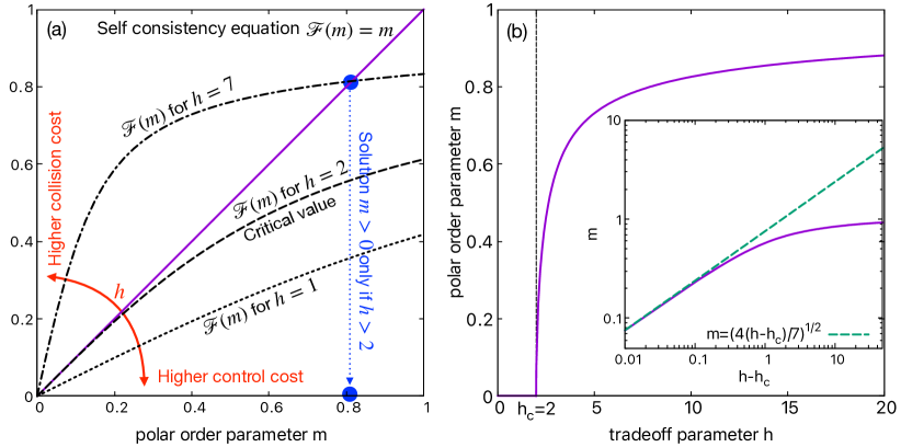
Figure 2: Self-consistency equation and polar order parameter: (a) graphical solution of Eq. (18), $\mathcal{F}(m)=m$ can only be satisfied with $m>0$ if $\mathcal{F}^{\prime}>1$, which requires the tradeoff parameter $h=(N-1)\,g_{1}/(D^{2}\,V)$ to be larger than $h_{c}=2$; (b) polar order parameter $m$ as a function of $h$, a second order phase transition takes place at $h=h_{c}$. The inset displays the asymptotic approximation (21) (green dashed line) showing the critical exponent to be $1/2$.

The function $\mathcal{F}(m)$, shown in Fig. 2a, depends on the parameter (see Table 1 for a handy summary of all the parameters of the problem and Table 2 for main relations and functions)

$$h=-\frac{q}{m}=\frac{\delta\,g_{1}}{D^{2}}\,,$$ (19)

which, besides containing all dependencies on the problem parameters $N,\;g_{1},\;D,\;V$, has a natural interpretation as the ratio between the parameters which control the importance of collision and control costs. For a clearer picture, we reintroduce $\alpha$ and write as $h=(g_{1}\,\delta)/(\alpha\,D^{2})$: at the numerator, $g_{1}$ is rescaled with particle density $\delta$ while, at the denominator, $\alpha$ is rescaled with diffusivity $D$. Note that the solution does not depend on $g_{0}$, as follows from homogeneity assumption. As graphically illustrated in Fig. 2a, Eq. (18) admits only the trivial solution with no polar order $m=m(h)=0$ for $0\leq h\leq h_{c}=2$, while a non-trivial solution emerges, via a second order transition to non-zero alignment ($m>0$) for $h>h_{c}$ (the critical value $h_{c}=2$ is derived in the next subsection by a perturbative expansion of the self-consistency equation). The numerically computed function $m(h)$ is shown in Fig. 2b. The polar oder parameter $m$ is zero up to the critical tradeoff value $h_{c}=2$, meaning that the alignment benefit outweighs the cost of control only for $h>h_{c}$. Therefore, for $h<h_{c}$, no control is applied and the system remains isotropic so that the average cost $\bar{C}$ (11) is equal to $C_{0}=\delta g_{0}/2$ while, as derived in D, for $h>h_{c}$, $\bar{C}$ is equal to

$$\bar{C}=C_{0}+\frac{1}{2}D^{2}\;[h\,m^{2}(h)+a(-m(h)\,h)]\,.$$ (20)

Note that, as anticipated, the constant $C_{0}$ is irrelevant to the optimization process (as a consequence of the mean field assumptions), while the remaining part depends only on the tradeoff parameter $h$, up to the $D^{2}$ prefactor.

In the following sections, we will give a more detailed description of both the critical behavior (for $h\to h_{c}=2$) and the strong coupling (large $h$) regime.

2.3 Critical behavior

As clear from Fig. 2, at the critical point $h=h_{c}=2$, there is a second order phase transition in the polar order parameter with exponent 1/2, a classical mean field value, which can be derived as follows. When $h=h_{c}^{+}$, we can solve Eqs. (15) and (16) perturbatively (see B), by expanding them in powers of $q=-m\,h$ for $q\to 0^{-}$ (small $m$ ansatz). Then, we can write Eq. (15) as $m\,(h-2)/2-7\,(m\,h)^{3}/64+o(m^{3})=0$, from which we obtain the asymptotic expression (for small $m$ or $\sqrt{h-h_{c}}$)

$$m=\sqrt{(4/7)\,(h-h_{c})}\,,$$ (21)

which, as shown in the inset of Fig. 2b, fully captures the critical behavior. In this regime, the desirability $\zeta$ can be approximated at leading order in $m$ as

$$\zeta(\theta)=\frac{1}{\sqrt{2\,\pi}}\left[1+\frac{h\,m(h)}{2}\,\cos\theta\right]\,.$$ (22)

Since the angular probability density function satisfies Eq. (14), agents directions are uniformly distributed but for a tiny $O(m)$ cosine modulation. Plugging Eq. (22) into Eq. (13), the optimal control at the critical point reads

$$f=-D\,h_{c}\,m\,\sin(\theta)+o(m)\,.$$ (23)

Moreover, exploiting the asymptotic expressions (46) for $a$ into Eq. (20), we can obtain the cost close to the critical point $h-h_{c}=0^{+}$:

$$\bar{C}-C_{0}=-(D^{2}/7)\,(h-h_{c})^{2}+o((h-h_{c})^{2})\,.$$ (24)

We conclude the investigation of the critical properties by studying the susceptivity to external perturbations, which is an important observable in multi-agent systems, both when considering artificial swarms control and biological collective behaviors, such as bird flocks or insect swarms. Indeed, the susceptivity describes the crowd sensitivity to fluctuations and/or external stimuli [33, 5]. In order to define the susceptivity, we need to specify an external field, and then compute the derivative of $m$ with respect to it. In our setting, the external field is represented by a small collective nudge of intensity $\epsilon$ in the direction $\hat{\theta}$, which formally amounts to adding a small per-agent reward in the cost function

$$\delta G_{i}=-\epsilon\;\cos(\theta_{i}-\hat{\theta})\,,$$ (25)

for aligning along the direction $\hat{\theta}$. The perturbation (25) breaks the isotropy favoring an average alignment in the preferred direction $\hat{\theta}$ (which, with no loss of generality, can be set to 0). Since $\hat{\theta}$ breaks the isotropy, and the system has no intrinsic preferred direction, we can deduce that the system will polarize along the preferred direction $\bar{\theta}=\hat{\theta}$. Therefore, susceptivity is then defined as

$$\chi(h)=\left.\frac{\partial m}{\partial\epsilon}\right|_{\epsilon=0}\,.$$ (26)

Essentially, the additional (negative) cost (25) induces the shift

$$q\mapsto q+\frac{2\epsilon}{D^{2}}\,,$$ (27)

which, plugged into Eq. (18), implicitly defines $m$ as a function of $\epsilon$, for any $h$. Then, by a straightforward application of Dini’s implicit function theorem (see E), we obtain the following result: when $h<h_{c}$, $\chi=2/[D^{2}\,(h_{c}-h)]$ holds exactly; close to the critical point ($h\to h_{c}^{+}$), $\chi=1/[D^{2}\,(h-h_{c})]+o(1/(h-h_{c}))$. Therefore, near the critical point, we have that the susceptivity diverges with $h\to h_{c}$ as

$$\chi\sim|h-h_{c}|^{-1}\,,$$ (28)

we notice that the critical exponent $1$ for the susceptivity is also quite standard in mean field theories. On the other hand, exactly at the critical point $h=h_{c}$, $m$ depends on $\epsilon$ as $m\sim 2\,\left[\frac{\epsilon}{7\,D^{2}}\right]^{1/3}$ and, hence, $m$ is a continuous but non differentiable function of $\epsilon$ at the critical point and, consequently, the susceptivity diverges as

$$\chi\sim\epsilon^{-2/3}\,.$$ (29)

The absence of a first order discontinuity implies that, at the critical point, an infinitesimal nudge is not enough to induce finite polarization in this kind of system. This a natural consequence of the continuous symmetry which is spontaneously broken even in absence of external perturbations. On the other hand, any small nudge is enough to fix the direction of the polarization vector.

2.4 Strong coupling

The strong coupling regime is identified by the condition $h\gg h_{c}$, which can be achieved with high density ($\delta=(N-1)/V\gg 1)$, with a high collision cost coefficient $g_{1}$ or with low noise $D$. In the large $h$ limit, we can analytically solve Eqs. (15) and (16) by exploiting a small oscillations ansatz which transforms the quantum pendulum into a quantum harmonic oscillator (50). As discussed in C, in this limit $m$ approaches to 1 asymptotically (strong alignment) as

$$m\sim 1-1/2\,\sqrt{h}\,.$$ (30)

The solution $\zeta$ becomes

$$\zeta(\theta)\sim\left(\frac{2\sqrt{h\,m(h)}}{\pi}\right)^{1/4}\,\exp(-\sqrt{h\,m(h)}\,\theta^{2})\,,$$ (31)

which via Eq. (14) implies that most agents are aligned along the average direction $\bar{\theta}$ and that - consistently with the small oscillations assumption - normal fluctuations vanish as $h^{-1/4}$. The associated asymptotic control is linear in $\theta$

$$f=-D\,\sqrt{h\,m(h)}\;\theta\,,$$ (32)

where $m\approx 1$ from (30). Note that, since this solution has been obtained in the small oscillations regime and, therefore, Eq. (32) is only accurate around $\theta=0$ which is, on the other hand, the only region which matters, since the probability of visiting other regions is exponentially suppressed. Exploiting the large $h$ asymptotics for the Mathieu characteristic function (51), one can easily obtain that the cost decreases approximately linearly with $h$ as $\bar{C}-C_{0}=D^{2}\,[-h/2+(3/4)\,\sqrt{h}]+o(\sqrt{h})$. Using the same scheme of the previous section, we can compute the susceptivity is this regime as well obtaining that $\chi$ (26) vanishes for large $h$ as $\chi\sim 1/[2\,D^{2}\,h^{3/2}\,m^{1/2}]$ (see E). Therefore, as we might have expected, the polar order strength $m$ is little responsive to external nudges, when it is already close to its maximum value 1.

3 Sinusoidal control vs optimal solution

3.1 Motivation

The optimal solution (23) to the collision avoidance problem in swarming active Brownian particles suggests that close to the critical point the optimal control is sinusoidal at leading order, i.e.

$$f=-D\,K\;\sin(\theta-\bar{\theta})\,,$$ (33)

with $K\approx h_{c}m$; notice that in Eq. (23) the mean field direction was put to zero ($\bar{\theta}=0$) for the sake simplicity and here restored for clarity. Interestingly, also the strong coupling optimal solution (32) is well approximated by the sinusoidal control (33): owing to the small oscillations property $|\theta-\bar{\theta}|\ll 1$, we can replace $\theta-\bar{\theta}$ with $\sin(\theta-\bar{\theta})$ in Eq. (32), obtaining $K\approx\sqrt{hm}$. Therefore, in both asymptotics ($h\to h_{c}^{+}$ and $h\to\infty$), Eq. (33) approximates the optimal control with a rescaled control strength $K$, which only depends on the parameter $h$ in both cases. This is quite noteworthy as the search of the optimal control is done without specifying the functional form of the control.

Remarkably, the control (33) is reminiscent of the mean field versions of the Kuramoto model [34] with zero natural frequencies, which is a paradigm for synchronization [35], and of the (time-continuous) stochastic Vicsek model [25, 26, 27, 24], which is a variant of one of the most popular models used for describing collective motions and swarming of self-propelled agents [2, 36]. In the mean field version of the latter [25, 26, 24], individual agents are driven by the approximate control $f_{V}=-R\,m\,\sin(\theta-\bar{\theta})$, corresponding to Eq. (33) upon defining

$$R=D\,K/m$$ (34)

whenever the polar order parameter $m=m(K,D,g_{1},V)$ is non zero.

Given the similarity, both in the critical and in the strong coupling limit, of the optimal control with the classical models discussed above it is worth to compare vis a vis the optimal control solution with the class of “sinusoidal control models” defined by Eq. (33). In particular, we aim at comparing the optimal control with the “best” sinusoidal control, defined by Eq. (33) with $K=K_{\star}$, with $K_{\star}$ being the value of $K$ that minimizes the average cost, given the parameters of the problem $(N,g_{1},V,D)$. As we will see, actually best sinusoidal model will depend on the familiar combination $h=(N-1)g_{1}/(VD^{2})$, so that $K_{\star}=K_{\star}(h)$ is a function of the tradeoff parameter $h$ only.

In the following subsection, after obtaining the best sinusoidal control, we briefly discuss the critical and strong coupling regimes and, then, we compare the optimal and best sinusoidal control for arbitrary tradeoff parameter values.

3.2 Best sinusoidal model

The dynamics of the heading direction for a generic agent with the sinusoidal control (33) is $d\theta=-K\,D\,\sin\theta dt+\sqrt{2D}\,d\xi$, where $\xi$ is the usual Wiener noise and where, again, we assume $\bar{\theta}=0$ for the sake of notation simplicity. Note that the above dynamics also describes the orientation of gravitactic (bottom-heavy) microorganisms in two dimensions, where $1/KD$ is the time scale with which the organism orients vertically upward oppositely to gravity [37, 38]. The Fokker-Planck equation associated with such dynamics, $\partial_{\theta}(-KD\sin\theta-D\partial_{\theta})\rho_{s}=0$ is solved by the Fisher-Von Mises distribution [39]

$$\rho_{s}(\theta)=\frac{1}{2\,\pi\,I_{0}(K)}e^{K\,\cos\theta}\,,$$ (35)

where $I_{\alpha}(z)$ is the modified Bessel function of the first kind of order $\alpha$ (briefly surveyed in F) and where the subscript $s$ is used to remind that it pertains to the sinusoidal control. Once the distribution is known, we can compute the polar order parameter as

$$m_{s}(K)=\int d\theta\rho_{s}(\theta)\cos\theta=\frac{I_{1}(K)}{I_{0}(K)}\,.$$ (36)

As stated, the best sinusoidal model is given by Eq. (33) with such $K_{\star}$ that minimizes the average cost (11). By plugging Eqs. (35) and  (33) into Eq. (11), after a few trigonometric passages combined with the identity (67), the sinusoidal control cost $\bar{C}_{s}$ can be written as

$$\bar{C}_{s}[K,D]=\int d\theta\,\rho_{s}\,C_{s}=C_{0}+D^{2}\left[-\frac{h}{2}\,m_{s}^{2}(K)+\frac{K}{2}\,m_{s}(K)\right]\,,$$ (37)

from which one can easily deduce that $K_{\star}=K_{\star}(h)$, as anticipated. Unfortunately, it is impossible to minimize the cost (37) analytically with respect to $K$, so we proceeded numerically. In Fig. 3a we show both $K_{\star}(h)$ as a function of the tradeoff parameter $h$.

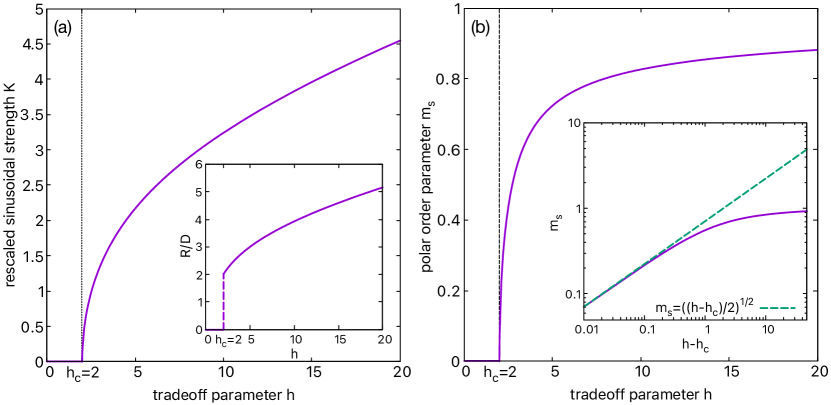
Figure 3: (a) Rescaled best sinusoidal control strength $K_{\star}$ as a function of the tradeoff parameter $h$. It is non-zero only for $h>h_{c}=2$, where a second order transition takes place. The inset shows the control strength $R_{\star}(h)=K_{\star}(h)/(m_{s}D)$ of the associated Vicsek mean field model, see Eq. (34). (b) polar order parameter $m_{s}$ as a function of $h$ for the best sinusoidal control. A second order phase transition is visible at $h=h_{c}=2$ with critical exponent $1/2$. The inset shows the asymptotic approximations (39) (green dashed line) valid close to the critical point. Notice the similarity with Fig. 2b.

Figure 3b displays the behavior of the polar order parameter $m_{s}=m_{s}(h)$ as a function of the tradeoff parameter $h$. Like in optimal case, the polar order parameter displays a second order phase transition at the same critical point $h=h_{c}=2$ and with the same critical exponent $1/2$. Indeed, as derived in G, by expanding the cost $\bar{C}_{s}$ for small $K$ one can derive that for $h-h_{c}\ll 1$, at leading order

$$K_{\star}\approx\sqrt{2(h-h_{c})}\,,$$ (38)

and that (see also inset of Fig. 3b)

$$m_{s}(h)\approx\sqrt{(1/2)(h-h_{c})}\,,$$ (39)

so that the sinusoidal control (33), near the critical point, features a rescaled strength $K_{\star}\approx h_{c}m_{s}$ which is similar to the optimal one (23). Note, however, that $m$ and $m_{s}$ are not fully equivalent. The previous expressions also imply that the best coupling $R_{\star}$ (Eq. (34)) from the Vicsek interpretation displays a first order discontinuity, as shown in the inset of Fig. 3a.

In spite of the similarities, the asymptotic dependence of $m_{s}$ on $h$ (for $h\to h_{c}^{+}$) differs by a pre-factor with respect to the optimal control: indeed comparing Eqs. (39) and (21) we have different prefactors $\sqrt{1/2}$ and $\sqrt{4/7}$, respectively which differ by a mere $6\%$. At a first glance this difference may seem surprising, but it can actually be rationalized by observing that the sinusoidal control is just a first order approximation to the optimal one while, as detailed below, the polar order parameter prefactor at criticality is determined by the first sub-leading order.

For the optimal control, we have derived the optimal critical behavior by expanding the self-consistency condition (18) $\mathcal{F}(m)=m$. The latter can be rewritten as $m=\langle\cos\theta\rangle_{m}$, which plays the same role as Eq. (36) for the sinusoidal model; $\langle[\ldots]\rangle_{m}$ is to remind that the probability density depends on the polarization itself as typical in self-consistent problems. As the control is odd w.r.t. the transformation $\bar{\theta}\mapsto\bar{\theta}+\pi$, it turns out that $\langle\cos\theta\rangle_{m}$ is odd in $m$. Consequently, close to the critical point (i.e. form small $m$) we can write $\langle\cos\theta\rangle_{m}=c_{1}\,hm+c_{k}\,(h\,m)^{k}+o((hm)^{k})$ with $k>1$ being an odd integer, which we know to be 3 (see e.g. Eq. (48)). Now, imposing the self-consistency condition $m=\langle\cos\theta\rangle_{m}$ yields

$$m\approx\left[\frac{1}{h^{k}\,c_{k}}\,(1-c_{1}\,h)\right]^{\frac{1}{k-1}}\,,$$ (40)

from which we deduce that the critical point $h_{c}=c_{1}^{-1}$ is solely determined by the first order and is, therefore, a leading order effect; the critical exponent is fixed by the value of $k$ (ordinal number of the first non-vanishing sub-leading order) as $1/(k-1)$ ($1/2$ in our case as $k=3$) and the prefactor is given by the sub-leading order prefactor $-c_{1}/(c_{k}\,h^{3})$. Since the optimal solution is sinusoidal at leading order, we expect $h_{c}=2$ to hold for both the optimal and best sinusoidal controls, by construction. The value of $k=3$ and, therefore, the critical exponent $1/2$, is fixed by the symmetry and should be the same for both models. However, any further equivalence is not obvious and, in particular, there is no specific reason for $c_{3}$ to be the same: they are actually different and this explains the difference in the prefactors discussed above.

Now we briefly discuss the strong coupling regime. For large $h$ (which implies large $K$), the Von-Mises distribution (35) is well approximated by the Gaussian

$$\rho_{K}=\sqrt{\frac{K}{2\pi}}\;\exp\left(-\frac{K}{2}\theta^{2}\right)\,,$$ (41)

and $\cos\theta\approx 1-\theta^{2}/2$. With such an approximation the self-consistency condition (36) yields $m_{s}=1-\frac{1}{2\,K}+o(1/K)$, which inserted into the cost (37) and minimizing with respect to $K$ gives

$$K_{\star}=\sqrt{h}+o(\sqrt{h})\,.$$ (42)

Consequently, the polar order parameter in the large $h$ limit is given by $m_{s}\approx 1-1/2\sqrt{h}$ as for optimal case (30).

The above discussion establishes a connection between sinusoidal and optimal model in the asymptotic regimes, but provides little insights into the intermediate region. In the next section, we further investigate the differences and similarities between optimal and best sinusoidal control.

3.3 Comparison between optimal solution and best sinusoidal model

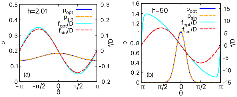
Figure 4: Comparison for the optimal and best sinusoidal model between the angular probability density function (left scale) and the control $f/D$ (right scale) for (a) $h=2.1$, i.e. close to the critical point, and (b) $h=50$, corresponding to the strong coupling regime. See the figure legend for the various curves.

Critical case comparison

For both models, below the critical point, $h<h_{c}$, no control is exerted as it is too expensive. Consequently, the stationary distribution of agents orientation is uniform in both cases. Near the critical point, $h-h_{c}=0^{+}$, the angular distribution remains approximately uniform and collision costs remain high, since collisions of anti-aligned particles are common. However, in this regime, tiny deviations of the optimal control from the sinusoidal one (see Fig. 4a) allows to slightly squeeze the distribution towards the alignment with the mean direction $\bar{\theta}=0$ in Fig. 4b and 5a. Therefore, the optimal model pays slightly more in the control cost to achieve a reduction of the collision cost w.r.t. the sinusoidal one, overall reducing the average cost, as shown in Fig. 6. In particular, close to the critical point, the cost difference between the optimal and sinusoidal model is

$$\Delta\bar{C}=\bar{C}-\bar{C}_{s}=-\frac{D^{2}}{56}\,(h-h_{c})^{2}+o((h-h_{c})^{2})\,,$$ (43)

as obtained by subtracting Eq. (72) from Eq. (24).

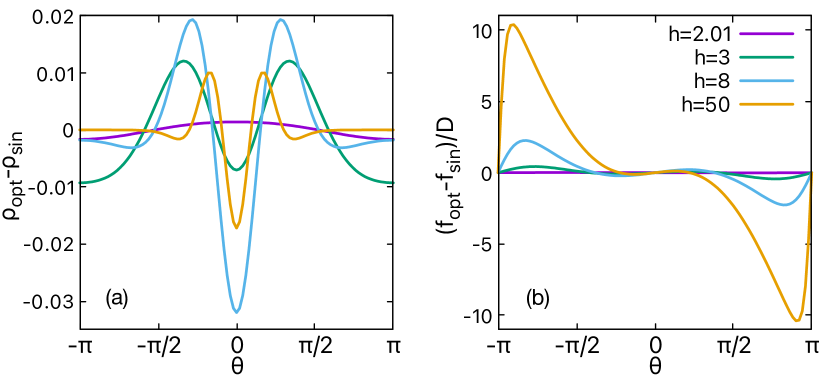
Figure 5: Differences between the optimal and best sinusoidal model: (a) angular probability density and (b) rescaled control, $(f(h)-D\,K_{\star}(h)\,\sin(\theta))/D$, for different $h$ as in figure legend.

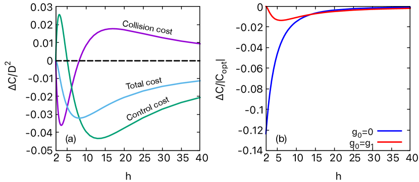
Figure 6: Cost comparison between optimal and best sinusoidal model: (a) rescaled average cost differences $\Delta\bar{C}=(\bar{C}-\bar{C}_{s})/D^{2}$ - total (cyan curve), collision (purple) and control (green)- plotted as universal functions of the tradeoff parameter $h$; (a) the relative cost difference $\Delta\bar{C}/|\bar{C}|$, as a function of the tradeoff parameter $h$ in two notable cases $g_{0}=0$ (pure alignment) and $g_{0}=g_{1}$ (pure collision).

Intermediate and strongly interacting regimes

As $h$ grows away from the critical point, both distributions shrink towards the origin, but not exactly in the same way. The best sinusoidal model distribution is more peaked both around the origin (strong alignment) and around $\pm\pi$ (strong anti-alignment), while intermediate values are less probable. This difference, highlighted in Fig. 5a, is the largest around $h=\hat{h}\approx 8$, which also corresponds to the the region where the difference between the total costs $\Delta\bar{C}$ is the largest, as shown in Fig. 6a. Just before $\hat{h}$, the optimal model outperforms the sinusoidal one in both control and collision costs. However, the collision costs advantage rapidly declines and, for large $h$, the edge of the optimal solution is preferred only due to lower control costs, while collision costs are higher. To understand the origin of these differences, we should look at the shape of the optimal control, which starts sinusoidal at $h-h_{c}=0^{+}$ and then approaches a sawtooth shape for $h\gg 1$ (see Fig. 5b and 4b). The strong control near $\pm\pi$ makes little difference in terms of costs, because the probability of exploring such region is exponentially suppressed. Indeed, both optimal and best sinusoidal distributions converge to the same Gaussian distribution with vanishing variance for large $h$ (see Fig. 4b). In other terms, the two seemingly different controls (Fig. 5b) only contribute with their linear approximation near the origin and are therefore equivalent, consistently with derivation of the previous section.

Rescaled-cost difference analysis

We have provided a detailed description of the differences between the two models. We should remark that all discrepancies we have highlighted are somehow small, since the two distributions never show significantly different shapes. Moreover, at the critical point, the critical exponents are the same and, finally, the polar order parameters are closely related for all $h$. The most delicate point is the cost difference: the universal behavior of the average cost difference as a function of $h$ (Fig. 6a) only emerges when rescaling with such difference with the factor $D^{2}$. In other terms, such difference can be made arbitrarily large as can be deduced, for instance, by rescaling $g\mapsto z\,g$ and $D\mapsto D\,\sqrt{z}$. Under this transformation, while $h$ does not change, the cost difference does, as $\Delta\bar{C}\mapsto z\,\Delta\bar{C}$.

Relative-cost difference analysis

The above observation implies that a sound analysis should take into account the relative difference $\Delta\bar{C}/\bar{C}$. Note, though, that such quantity depends on the constant $C_{0}$ and thus on $g_{0}$ (which otherwise play no role in the optimization process). However, as discussed $g_{0}$ relates to the interpretation of the model, thus it is not possible to give a universal description. We can briefly consider some notable cases: $g_{0}=0$ and $g_{0}=g_{1}$ which represent a pure alignment and collision problem, respectively. In the former case, $\Delta\bar{C}/|\bar{C}|$ is 0 for $h<h_{c}$ and then (first order discontinuity) jumps to $-1/8$ at $h=h_{c}$ (see Fig. 6b) and finally vanishes to zero for $h\to\infty$. Note, however, that the maximal relative cost difference at $h=h_{c}^{+}$ is obtained in a limit in which both $\Delta\bar{C}$ and, mostly important, $\bar{C}$ itself vanishes (see Eqs. (43) and (24) with $C_{0}=0$). On the other hand, in the $g_{0}=g_{1}$ case, we have that $\bar{C}=C_{0}\neq 0$ at $h=h_{c}$ meaning that the even the cost of isotropic random collisions is not zero. Consequently, since the denominator never vanishes, we have $\Delta\bar{C}/|\bar{C}|\to 0$ for $h\to h_{c}^{+}$. Similarly, for $h\to\infty$, it is easy to see that $\Delta\bar{C}/|\bar{C}|\to 0$, as the two models are equivalent at leading order. Therefore, the maximal relative difference is realized for some $h\in(h_{c},\infty)$: a numerical test shown in Fig. 6b reveals that this is realized at $h\approx 6$ with $\Delta\bar{C}/|\bar{C}|\approx-0.0135$. By considering both the rescaled and the relative cost difference analysis, we can conclude that the sinusoidal model is always a good approximations for the optimal solution in realistic scenarios.

4 Discussion

We have shown by means of optimal control techniques, that the optimal behavior for collision-avoiding active particles can be characterized by a tradeoff parameter $h$ between collision and control costs, and that the polarization of the system undergoes a phase transition in the mean-field regime. The possibility of approaching this problem analytically, albeit in an approximate form, provided insights into the features of the optimal solution and a comprehensive statistical characterization. Moreover, we found that the optimal behavior, both close to the transition and for large tradeoff values, is well approximated by a mean-field version of the kinetic Vicsek model [25, 26, 24] which also displays a second order transition. Therefore, such model, whose short range version was mainly derived from phenomenology, turns out to be a quasi-optimal solution for the collision-avoidance task, given appropriate parameters. Clearly, when working with task-oriented agents, as in biological systems or robotics, being close to optimality is a highly desirable feature. The optimal control framework is therefore a very valuable tool not just for discovering new optimal models, but also for assessing the quality of existing ones with respect to some performance criteria. Moreover, in accordance with previous works, e.g. Ref. [17] where known chemotactic behaviors were found to be optimal solutions to target search problem, our findings suggest that optimal control formalism can, at least in some cases, provide a theoretical ground to interpret some biological solutions in situations where specific tasks need to be solved.

While our analysis was restricted to a single scenario, the same approach could be successfully carried in different settings to explore other classes of collective behaviors, for instance allowing for linear acceleration or for particles of finite sizes. Also, remaining in the context of mean-field Vicsek-like models, it would be interesting to explore how different kinds of noise can influence the optimal solution. Another interesting outlook would be to go beyond the mean field approximation, either analytically or numerically, by introducing a spatial structure.

Appendices

Appendix A Mathieu functions

Mathieu functions are solutions of eigenvalue Schrödinger equation for the quantum pendulum, which is customarily written as

$$\zeta^{\prime\prime}+(a-2\,q\,\cos(2\,y))\,\zeta=0\,,$$ (44)

with $y\in[-\pi/2,\pi/2]$, and where $q$ is some constant and $a$ is (minus) the eigenvalue (the “energy”). For any $q$, the eigenvalues $a_{k}(q)$ depend on a parameter $k$ and are called Mathieu characteristic function. By imposing boundary conditions, $k>0$ becomes and integer representing the ordinal number of the energy level: if $q<0$ then $-a_{k}(q)<-a_{k+1}(q)$. The eigenfunctions $\mathpzc{m}_{k}$ are either even $\mathpzc{ce}_{k}=\mathpzc{m}_{2k}$ or odd $\mathpzc{se}_{k}=\mathpzc{m}_{2k+1}$. Since we are only interested in the ground state with periodic boundary conditions, we focus on $k=0$. The eigenvalue is $a(q):=a_{0}(q)$ (main text notation) and the eigenfunction $\zeta=\mathpzc{ce}_{0}(a(q),q)$. For further details, see for instance Refs. [31, 32, 40].

Appendix B Optimal solution near the critical point

In this appendix, we derive the mean-field solution of the system of equations (15) and (16) near the critical point. We start from the Mathieu equation (44) and we observe that $m\to 0$ implies $q=-h\,m\to 0$ (see Table 1) for finite $h$. We solve the equation perturbatively by expanding the solution $\zeta$ and the eigenvalue $a$ in power series of $q$, by writing

$$\begin{dcases}\zeta=\zeta_{0}+\zeta_{1}+\zeta_{2}+\zeta_{3}+\zeta_{4}+o(q^{4})\\ a=a_{0}+a_{1}+a_{2}+a_{3}+a_{4}+o(q^{4}).\end{dcases}$$ (45)

where $a_{k}=O(q^{k})$ and $\zeta_{k}=O(q^{k})$ (for instance in $C_{\infty}$ norm). At any order $k$, we impose $\zeta^{\prime\prime}+(a-2\,q\,\cos(2\,y))\,\zeta=o(q^{k})$ and $\int_{-\pi/2}^{\pi/2}dy\,\zeta^{2}=1+o(q^{k})$, starting from order 0 to 4. Clearly, for any $k$, $\zeta_{k}$ and $a_{k}$ only depend on $\{\zeta_{s}\,,a_{s}\}_{s<k}$. From this procedure, we find that the eigenvalue is

$$a(q)=-\frac{1}{2}\,q^{2}+\frac{7}{128}\,q^{4}+o(q^{4}),$$ (46)

while the eigenfunction can be written as the following expansion in harmonics

$$\zeta=\frac{1}{\sqrt{\pi}}\left[1-\frac{q^{2}}{16}+\left(-\frac{q}{2}+\frac{11\,q^{3}}{128}\right)\,\cos(2\,y)+\frac{q^{2}}{32}\,\cos(4\,y)-\frac{q^{3}}{1152}\,\cos(6\,y)\right]+o(q^{3}).$$ (47)

From expansion (47), the self-consistency condition (18) can be written as

$$m=\int_{-\pi/2}^{\pi/2}dy\,\zeta_{0}^{2}\,\cos(2\,y)=\frac{h\,m}{2}-\frac{7\,(m\,h)^{3}}{64}+o(m^{3})\,,$$ (48)

which has 3 solutions: the trivial one $m=0$, an unphysical solution $m<0$ and

$$m\sim\sqrt{\frac{32}{7\,h^{3}}}\sqrt{h-2}\sim\sqrt{\frac{4}{7}}\sqrt{h-2}$$ (49)

which is only well defined for $h>h_{c}=2$, where a second order phase transition occurs. This yields the asymptotic behavior and the critical exponent $1/2$.

Appendix C Optimal solution for large $h$.

To study the $h\gg h_{c}$ regime, we assume $m\approx 1$, from which it follows that $q(h)=-h\,m(h)$ becomes large negative. For large $q$, then both $\zeta$ and $\rho$ are peaked around $y=0$ and, therefore, we can assume a regime of small oscillations $|y|\ll 1$. Then, by expanding $\cos(2\,y)\approx 1-2\,y^{2}$, as one would expect from physics, Eq. (44)) reduces to the well-known Schrödinger equation of the quantum harmonic oscillator:

$$-\frac{1}{2}\zeta^{\prime\prime}+\frac{1}{2}\underbrace{(-4\,q)}_{\omega_{0}^{2}}\,y^{2}\,\zeta=\underbrace{\frac{a-2\,q}{2}}_{E}\,\zeta.$$ (50)

From the ground state eigenvalue solution $E_{0}=\omega_{0}/2$, we get the large $q$ approximation of the characteristic function $a$

$$a(q)\approx 2\,q+2\,\sqrt{-q}\mbox{ for }q\ll-1\,.$$ (51)

Conversely, from the ground state eigenfunction $\exp(-\omega_{0}/2\,y^{2})$, we get

$$\zeta=\left(\frac{2\sqrt{-q}}{\pi}\right)^{1/4}\;\exp(-\sqrt{-q}\,y^{2})$$ (52)

where we have extended the domain of $y$ from $[-\pi/2,\pi/2]$ to $(-\infty,\infty)$ by enforcing normalization $\int_{-\infty}^{\infty}dy\;\zeta^{2}(y)=1$. We can then rewrite Eq. (18) as $\int_{-\infty}^{\infty}dy\;\zeta^{2}(y)\,\cos(2\,y)=m$ which becomes

$$m=e^{-\frac{1}{2\sqrt{hm}}}.$$ (53)

Hence, if $h\to\infty$, then $m\to 1$, validating our small-oscillations ansatz. More precisely

$$1-m\sim\frac{1}{2\,\sqrt{h}}\mbox{ for }h\to\infty\,.$$ (54)

Appendix D Proof of equation (20)

The mean field costs (11) can be written as

$$\bar{C}-C_{0}=-\frac{D^{2}\,h}{2}\,m\int d\theta\,\zeta^{2}\,\cos\theta+2\,D^{2}\,\int d\theta\,\zeta^{2}\,(\partial_{\theta}\ln\zeta)^{2}=-\frac{D^{2}\,h}{2}\,m^{2}+2\,D^{2}\,\int d\theta\,(\partial_{\theta}\zeta)^{2}.$$ (55)

We can apply partial integration to the control cost term $\int d\theta\,(\partial_{\theta}\zeta)^{2}=-\int d\theta\,\zeta\,\partial_{\theta}^{2}\zeta$. By using the Mathieu equation 44, we can write $\int d\theta\,(\partial_{\theta}\zeta)^{2}=a/4+m^{2}\,h/2$. Equation (20) follows from a straightforward substitution.

Appendix E Proofs of the expressions for the susceptivity

Consider an external field as defined in Eq. (25). The self consistency condition (18) implicitly defines the polar oder parameter $m=m(h,\epsilon)$ as

$$\mathcal{F}(m(h,\epsilon))=m(h,\epsilon).$$ (56)

Upon defining $\tilde{\mathcal{F}}=m-\mathcal{F}$, Dini implicit function theorem allows to compute the susceptivity as

$$\chi(h)=\left.\frac{\partial m}{\partial\epsilon}\right|_{\epsilon=0}=-\frac{\left.\frac{\partial\tilde{\mathcal{F}}}{\partial\epsilon}\right|_{\epsilon=0}}{\left.\frac{\partial\tilde{\mathcal{F}}}{\partial m}\right|_{\epsilon=0}}.$$ (57)

though, in some cases, there is a shorter procedure. We consider the following four scenarios.

• $h<h_{c}$. In this case, we can assume that, unless there is some discontinuity, $\lim_{\epsilon\to 0}m(h,\epsilon)=0$. Hence, assuming both $\epsilon$ and $m$ small, Eq. (56) can be expanded as

  $$-\frac{(h-2)\,m+2\,\epsilon/D^{2}}{2}+\frac{7\,(m\,h+2\,\epsilon/D^{2})^{3}}{64}+o((m\,h+2\,\epsilon/D^{2})^{3})=0\,.$$ (58)

  Then we can either use Dini’s theorem or simply observe that $\mathcal{F}=0$ at leading order implies $m=2\epsilon/[D^{2}\,(2-h)]$ and, therefore

  $$\chi=\frac{2}{D^{2}\,(h_{c}-h)}\,,$$ (59)

  holds exactly in this region.

• $h=h_{c}$. We can again use the ansatz $\lim_{\epsilon\to 0}m(h,\epsilon)=0$ along with Eq. (58). Then, either applying Dini’s theorem, or observing that, since $h-2$ is zero exactly, leading order in $\epsilon$ must match leading order in $m$, which is $m^{3}$. Hence, we immediately get

  $$m\sim 2\,\left[\frac{\epsilon}{7\,D^{2}}\right]^{1/3}\,,$$ (60)

  thus, at the critical point, $m(\epsilon)$ in continuous in $\epsilon$ but non differentiable.

• $h=h_{c}^{+}$. As in the critical regime, it remains valid that the nudge selects the direction in which the symmetry is broken since other choices would be sub-optimal. Here $\lim_{\epsilon\to 0}m(h,\epsilon)=m(h)>0$, however, as long as $h$ is close to $h_{c}$, we can still use expansion (58). From Eq. (49) we can write $m(h)=\sqrt{(4/7)\,(h-2)}+\delta m$, with $\delta m\ll 1$ and match leading order of $\delta m$ and $\epsilon$. As a result, we get

  $$\chi\sim\frac{1}{D^{2}\,(h_{c}-h)}\,.$$ (61)

• $h\gg h_{c}$. Using Eq. (53), the self consistency equation (18) becomes

  $$m-e^{-\frac{1}{2\,\sqrt{h\,m+2\,\epsilon/D^{2}}}}=0\,,$$ (62)

  and a straightforward application of Dini’s theorem yields

  $$\chi\sim\frac{1}{2\,D^{2}\,h^{3/2}\,{m}^{1/2}}\,.$$ (63)

Appendix F Modified Bessel function of the first kind

Modified Bessel functions of the first kind are non decreasing solution of the modified Bessel equation:

$$z^{2}\,I_{n}^{\prime\prime}+z\,I_{n}^{\prime}-(z^{2}+n^{2})\,I_{n}=0$$ (64)

We report a few identities we have used in the main text

$$I_{0}(z) =\int_{-\pi}^{\pi}d\theta\,e^{z\cos\theta}$$ (65)

$$I_{0}^{\prime}(z) =I_{1}(z)=\int_{-\pi}^{\pi}d\theta\,\cos\theta\,e^{z\cos\theta}$$ (66)

$$I_{0}^{\prime\prime}(z) =I_{0}(z)-\frac{1}{z}\,I_{1}(z)=\int_{-\pi}^{\pi}d\theta\,\cos^{2}\theta\,e^{z\cos\theta}$$ (67)

For further details, see [40].

Appendix G Best sinusoidal control near the critical point

To obtain some analytical insights into the critical behavior of the best sinusoidal model, we follow the same logic as for the optimal model (B). The main difference is that, instead of expanding for small $q$, we expand for small $K$. In the end, the procedures appear to be equivalent as they are both expansion in $\sqrt{h-h_{c}}$. First, we can expand (35) and get

$$\rho_{s}=\frac{1}{2\,\pi}\left(1+K\cos\theta+\frac{K^{2}}{4}(2\,\cos^{2}\theta-1)\right.\\ \left.+\frac{K^{3}}{12}(2\,\cos^{3}\theta-3\cos\theta)+\frac{K^{4}}{192}(9-24\,\cos^{2}\theta+8\,\cos^{4}\theta)\right)+o(K^{4})$$ (68)

Then, by using Eqs. (36) and (68), the average total cost (37) can be written explicitly as

$$\bar{C}_{s}-C_{0}=D^{2}\left[\left(\frac{1}{4}-\frac{h}{8}\right)\,K^{2}+\frac{h-1}{32}\,K^{4}\right]+o(K^{4})$$ (69)

A positive $K=K_{\star}$ which minimizes the previous expression exists only for $h>h_{c}=2$ and its asymptotic expression near $h_{c}$ is

$$K_{\star}\sim\sqrt{2\,(h-2)}\,,$$ (70)

which plugged into Eq. (36) yields

$$m\sim\sqrt{\frac{1}{2}(h-h_{c})}\,.$$ (71)

It follows from Eqs. (70) and (69) that

$$\bar{C}_{s}-C_{0}=-\frac{D^{2}}{8}\,(h-h_{c})^{2}+o((h-h_{c})^{2})\,.$$ (72)

References

References

- [1] Okubo A 1986 Adv. Biophys. 22 1–94
- [2] Vicsek T and Zafeiris A 2012 Phys. Rep. 517 71–140
- [3] Wolgemuth C W 2008 Biophys. J. 95 1564–1574
- [4] Sullivan R T 1981 Fla. Entomol. 64 44–65
- [5] Cavagna A, Conti D, Creato C, Del Castello L, Giardina I, Grigera T S, Melillo S, Parisi L and Viale M 2017 Nat. Phys. 13 914–918
- [6] Cavagna A, Giardina I and Grigera T S 2018 Phys. Rep. 728 1–62
- [7] Attanasi A, Cavagna A, Del Castello L, Giardina I, Grigera T S, Jelić A, Melillo S, Parisi L, Pohl O, Shen E and Viale M 2014 Nature Phys. 10 691–696
- [8] Pitcher T J 1983 Anim. Behav. 31 611–613
- [9] Pavlov D and Kasumyan A 2000 J. Ichthyol. 40 S163
- [10] Reynolds C W 1987 Flocks, herds and schools: A distributed behavioral model Proceedings of the 14th annual conference on Computer graphics and interactive techniques pp 25–34
- [11] Vicsek T, Czirók A, Ben-Jacob E, Cohen I and Shochet O 1995 Phy. Rev. Lett. 75 1226
- [12] Turgut A E, Çelikkanat H, Gökçe F and Şahin E 2008 Swarm. Intell. 2 97–120
- [13] Virágh C, Vásárhelyi G, Tarcai N, Szörényi T, Somorjai G, Nepusz T and Vicsek T 2014 Bioinspir. Biomim. 9 025012
- [14] Todorov E 2009 Proc. Natl. Acad. Sci. U.S.A. 106 11478–11483
- [15] Lasry J M and Lions P L 2007 Japanese J. Math. 2 229–260
- [16] Ullmo D, Swiecicki I and Gobron T 2019 Phys. Rep. 799 1–35
- [17] Pezzotta A, Adorisio M and Celani A 2018 Phys. Rev. E 98 042401
- [18] Hongler M O 2020 J. Dyn. Games 7 1
- [19] Durve M, Peruani F and Celani A 2020 Phys. Rev. E 102 012601
- [20] Romanczuk P, Bär M, Ebeling W, Lindner B and Schimansky-Geier L 2012 Europ. Phys. J. Spec. Top. 202 1–162
- [21] Bechinger C, Di Leonardo R, Löwen H, Reichhardt C, Volpe G and Volpe G 2016 Rev. Mod. Phys. 88 045006
- [22] Mora T and Bialek W 2011 J. Stat. Phys. 144 268–302
- [23] Farrell F D C, Marchetti M C, Marenduzzo D and Tailleur J 2012 Phys. Rev. Lett. 108 248101
- [24] Chepizhko O, Saintillan D and Peruani F 2021 Soft Matter 17 3113–3120
- [25] Peruani F, Deutsch A and Bär M 2008 Europ. Phys. J. Spec. Top. 157 111–122
- [26] Chepizhko A and Kulinskii V 2009 The kinetic regime of the vicsek model AIP Conf. Proc. vol 1198 pp 25–33
- [27] Chepizhko A and Kulinskii V 2010 Physica A 389 5347–5352
- [28] Howard R A and Matheson J E 1972 Manage. Sci. 18 356–369
- [29] Dvijotham K and Todorov E 2011 A unified theory of linearly solvable optimal control Proceedings of the 27th Conference on Uncertainty in Artificial Intelligence (UAI 2011) vol 1 pp 25–34
- [30] Pontryagin L S 2018 Mathematical theory of optimal processes (Routledge)
- [31] Brimacombe C, Corless R M and Zamir M 2020 arXiv preprint arXiv:2008.01812
- [32] Gutiérrez-Vega J C, Rodrıguez-Dagnino R, Meneses-Nava M and Chávez-Cerda S 2003 Am. J. Phys. 71 233–242
- [33] Bialek W, Cavagna A, Giardina I, Mora T, Silvestri E, Viale M and Walczak A M 2012 Proc. Natl. Acad. Sci. U.S.A. 109 4786–4791
- [34] Kuramoto Y 1975 Self-entrainment of a population of coupled non-linear oscillators International symposium on mathematical problems in theoretical physics (Springer) pp 420–422
- [35] Acebrón J A, Bonilla L L, Vicente C J P, Ritort F and Spigler R 2005 Rev. Mod. Phys 77 137
- [36] Ginelli F 2016 Eur. Phys. J. Spec. Top. 225 2099–2117
- [37] Pedley T J and Kessler J 1987 Proc. R. Soc. B 231 47–70
- [38] Cencini M, Franchino M, Santamaria F and Boffetta G 2016 J. Theor. Biol. 399 62–70
- [39] Mardia K V and Jupp P E 2009 Directional statistics vol 494 (John Wiley & Sons)
- [40] Gradshteyn I S and Ryzhik I M 2014 Table of integrals, series, and products (Academic press)