Total-Variation - Fast Gradient Flow and Relations to Koopman Theory

Abstract

The space-discrete Total Variation (TV) flow is analyzed using several mode decomposition techniques. In the one dimensional case, we provide analytic formulations to Dynamic Mode Decomposition (DMD) and to Koopman Mode Decomposition (KMD) of the TV flow and compare the obtained modes to TV spectral decomposition. We propose a computationally efficient algorithm to evolve the one-dimensional TV flow. A significant speedup by three orders of magnitude is obtained, compared to iterative minimizations. A common theme, for both mode analysis and fast algorithm, is the significance of phase transitions during the flow, in which the subgradient changes.

We explain why applying DMD directly on TV-flow measurements cannot model the flow or extract modes well. We formulate a more general method for mode decomposition that coincides with the modes of KMD. This method is based on the linear decay profile, typical to TV-flow. These concepts are demonstrated through experiments, where additional extensions to the two-dimensional case are given.

List of abbreviations

ADMM	Alternating Direction Method of Multipliers
DMD	Dynamic Mode Decomposition
FGD	Fastest Gradient Descent
KEF	Koopman Eigenfunction
KMD	Koopman Mode Decomposition
PDE	Partial Differential Equation
RDMD	Rescaled Dynamic Mode Decomposition
SVD	Singular Vector Decomposition
TV	Total Variation

List of variables

$P(\cdot)$	a proper nonlinear operator
$\psi(t)$	The solution of a nonlinear PDE
$t$	The time variable
$t(\psi)$	The inverse function from the observations $\psi$ back to the time $t$
$\varphi_{\mathcal{K}}(\psi)$	Koopman Eigenfunction (KEF)
$\bm{v}_{i}$	A Koopman mode
$a_{\lambda_{i}}(t)$	The decay profile typical to the dynamical system
$J_{TV}$	Total variation
$J_{iso}$	Isotropic total variation
$J_{ani}$	Anisotropic total variation
$T_{i}$	The time point at which the subgradient of TV-flow changes for the $i$th time.
$p$	a negative subgradient
$p_{i}$	The negative subgradient of the TV-flow for $t\in[T_{i},T_{i+1})$
$p^{i}$	The negative subgradient in the $i$th extremum of the signal
$p^{(i)}$	The value of the $i$th pixel in the negative subgradient $p$
$\tau$	The reparametrized time variable
$\varphi_{i}$	TV spectral component
$\xi_{1},\xi_{2}$	Modes resulting from the rescaled TV-flow
$\phi_{1},\phi_{2}$	Modes resulting from DMD applied on the rescaled TV-flow

1 Introduction

Dimensionality reduction is one of the most challenging tasks in data analysis. For flows, the general aim is to find a low dimensional representation of the spatial data (modes) and the corresponding temporal evolution zhang2020evaluating . This allows much better understanding and facilitates fast and efficient processing of the signal. The spatio-temporal decomposition is commonly used in many disciplines such as fluid dynamics, signal analysis and computational physics, to name a few. In this work, we bridge between the TV spectral decomposition from signal processing and its connection to Koopman theory and its applications.

In order to study nonlinear dynamics, Koopman theory koopman1931hamiltonian is increasingly employed. It allows a linear representation of nonlinear flows , also referred to as KMD mezic2005spectral . Since in the general case the representation is infinite-dimensional, in practice, a finite dimensional approximation is used. In fluid dynamics, Dynamic Mode Decomposition (DMD) is a data-driven method to approximate KMD schmid2010dynamic . Since DMD approximates a linear dynamical system it can be viewed as an exponential data fitting algorithm askham2018variable . DMD has become a popular and practical analysis tool, however, it suffers from some inherent flaws cohen2020introducing ; cohen2021examining ; rosenfeld2021singular ; elmore2021learning . These drawbacks are emphasized in zero-homogeneous evolutions such as the TV flow.

The TV functional has been extensively used in image processing and computer vision, as it allows the preservation of edges (discontinuities). The respective steepest descent, termed TV-flow, has been studied thoroughly in the last two decades tvFlowAndrea2001 ; steidl2004equivalence ; steidl2005relations ; brox2003equivalence ; chambolle2004algorithm ; bonforte2012total ; tvFlowAndrea2001 ; bellettini2002total . A list of the main attributes of TV flow in a one-dimensional signal is summed up in brox2006tv . Two of its main attributes are that the flow decays piecewise linearly and that it has a finite support in time. The above studies lay the foundation to the TV nonlinear spectral framework (spectral TV) gilboa2013spectral ; gilboa2014total ; burger2016spectral ; gilboa2016nonlinear ; bungert2021nonlinear ; brokman2021nonlinear ; fumero2020nonlinear . A main challenge in accurately using TV flow is the computational load in calculating the subgradient. For an accurate calculation, often a convex optimization problem (such as chambolle2004algorithm ) is solved at each step. In order to obtain a full spectral TV decomposition of a signal, one has to compute the entire TV flow until extinction. This motivates us to explore fast methods to accomplish the task.

In this work, we apply the theory of Koopman operator and its applications on the TV-flow. We begin by formulating the analytic solution of TV-flow for one-dimensional signals and propose a fast algorithm to solve the flow. We first examine Rescaled Dynamic Mode Decomposition (RDMD) cohen2020modes which was recently proposed as an improved version of DMD for homogeneous flows (such as $p$-Laplacian flows kuijper2007p , where the operator of the dynamics is homogeneous of degree $p-1$). However, since there are subgradient phase transitions in TV-flow, RDMD is limited. To address this problem we suggest a new piecewise mode decomposition technique. It is based on the linear decay profile typical to the flow. We show it coincides with KMD and can perfectly model the dynamics through piecewise linear segments. We show the direct relations of the obtained modes to spectral TV decomposition gilboa2014total . A shorter version of this work was first presented in a conference cohen2021Total . Here, additional theory and experiments are shown, and a two-dimensional extension is presented.

2 Preliminaries

In this section, we summarize the definitions and methods relevant to this work.

2.1 Koopman Eigenfunctions

Let us consider the following nonlinear dynamical system

$$\frac{d}{dt}\psi=P(\psi),$$ (1)

where $P(\cdot)$ is a proper nonlinear operator. The observation $\psi$ belongs to $\mathbb{R}^{M}$. We also denote the time derivative with the subscript $\{\cdot\}_{t}$ for simplicity.

Let $g:\mathbb{R}^{M}\to\mathbb{R}$ be a measurement of $\psi$. Bernard Osgood Koopman argued that a Hamiltonian system has measurements evolving linearly under the dynamical regime koopman1931hamiltonian . These measurements, termed as Koopman Eigenfunctions (KEFs), admit the following relation,

$$\frac{d}{dt}\varphi_{\mathcal{K}}(\psi(t))=\lambda\varphi_{\mathcal{K}}(\psi(t)),$$ (2)

where $\varphi(\psi)$ is a KEF and $\lambda$ is the respective eigenvalue. Recently, part of the authors formulated necessary and sufficient conditions for the existence of such measurements cohen2021examining . It was shown that if the solution of the system, $\psi(t)$, is injective then the measurement $\varphi$ gets the form of,

$$\varphi_{\mathcal{K}}(\psi)=\varphi_{\mathcal{K}}(\psi(0))e^{\lambda t(\psi)},$$ (3)

where $t(\psi)$ is the inverse function from the observations $\psi$ back to the time $t$. For further details see cohen2021examining .

2.2 Koopman Mode Decomposition

Koopman Mode Decomposition (KMD) is a representation of dynamical systems based on KEFs mezic2005spectral . Namely, the state space $\psi$ can be expressed as,

$$\psi(t)=\sum_{i=1}^{\infty}\bm{v}_{i}\varphi_{\mathcal{K}_{i}}(t),$$ (4)

where $\varphi_{i}(t)$ is a KEF and $\bm{v}_{i}$ is the corresponding vector, referred to as Koopman mode. When the dynamic is nonlinear the decomposition may be infinite. In practice, a finite approximation method is used. The most common one is DMD.

2.3 Dynamic Mode Decomposition

Dynamic Mode Decomposition (DMD) is a data-driven algorithm to approximate KMD. Given a set of samples of the dynamic, a linear relation is formulated that approximates the generating process of the set. Commonly, the formulation is performed in a lower dimensional space. The output is triplets representing the main spatial structures (modes), their amplitudes (coefficients), and the respective time changes (eigenvalues). To recap, the three main steps of this algorithm are: 1. Dimensionality reduction, 2. Optimal linear mapping, and 3. System reconstruction . The output is modes, eigenvalues and coefficients schmid2010dynamic .

2.4 Decay profile profile decomposition with Koopman modes

We summarize below a different decomposition method, suggested in cohen2021examining , which is relevant to this work. Let us assume that the dynamical system can be formulated as,

$$\psi(t)=\sum_{i=1}^{L}\bm{v}_{i}a_{\lambda_{i}}(t),$$ (5)

where $a_{\lambda_{i}}(t)$ is the decay profile typical to the dynamical system and characterized by a parameter (or set of parameters) $\lambda_{i}$ and $\bm{v}_{i}$ is a spatial structure. In matrix notations,

$$\psi(t)=V\bm{{a}_{\lambda}}(t),$$ (6)

where $\bm{a}_{\bm{\lambda}}(t)=\begin{bmatrix}a_{\lambda_{1}}(t)&\cdots&a_{\lambda_{L}}(t)\end{bmatrix}^{T}$ and $V$ is a matrix with the modes as its columns. If the decay profile is monotone, the inverse mapping exists and can be expressed as,

$$\bm{t}(\psi)=\bm{a}_{\bm{\lambda}}^{-1}\left((V^{T}V)^{-1}V^{T}\psi\right),$$ (7)

where $\bm{a}_{\bm{\lambda}}^{-1}(\cdot)=\begin{bmatrix}a_{\lambda_{1}}^{-1}(\cdot)&\cdots&a_{\lambda_{L}}^{-1}(\cdot)\end{bmatrix}^{T}$. Note that $\bm{t}$ is a vector of inverse mapping. Therefore, the Koopman eigenfunctions are,

$$\bm{\varphi_{\mathcal{K}}}(\psi)=\exp\{\bm{a}_{\bm{\lambda}}^{-1}\left((V^{T}V)^{-1}V^{T}\psi\right)\},$$ (8)

where $\bm{a}_{\bm{\lambda}}^{-1}(\cdot)=\begin{bmatrix}a_{\lambda_{1}}^{-1}(\cdot)&\cdots&a_{\lambda_{L}}^{-1}(\cdot)\end{bmatrix}^{T}$.

The general mode decomposition algorithm is data-driven. We mention here only the part in the algorithm revealing the spatial structures. For the rest of the algorithm, we refer the reader to cohen2021examining . Given the data matrix, $\Psi$, we initialize the decay profile dictionary, $\mathcal{D}$. The columns of the matrix are samples of the decay vector $\bm{a_{\lambda}}(t)$. We minimize the expression,

$$\norm{\Psi-VD}^{2}_{F}$$ (9)

over $V$, where $V$ is sparse columns-wise (the substrict $F$ denotes the Frobenius norm) . Then, we construct the matrices $\hat{V}$ and $\hat{D}$. $\hat{V}$ contains the non-zero (or non-negligible) modes (vectors in $V$) and $\hat{D}$ contains the respective decay profiles. Note that, the mode set $\{\bm{v}_{i}\}$ is proved to be the set of Koopman modes cohen2021examining .

2.5 Total Variation Spectral Decomposition

2.5.1 TV functional

One dimensional signal.

The TV functional of a one dimensional function is defined by,

$$J_{TV}(\psi)=\langle\absolutevalue{\nabla\psi},1\rangle,\quad\psi\in\mathbb{R}^{M},$$ (10)

where $\nabla$ is the discrete gradient operator. (for more details we refer the reader to chambolle2010introduction ).

Two dimensional signal.

For a two dimensional function, the definitions of isotropic and anisotropic TV, respectively, are,

$$\begin{split}J_{iso}(\psi)&=\langle\norm{\nabla\psi}_{2},1\rangle=\langle\sqrt[]{\absolutevalue{D_{x}\psi}^{2}+\absolutevalue{D_{y}\psi}^{2}},1\rangle,\quad\psi\in\mathbb{R}^{M\times K}\\ J_{ani}(\psi)&=\langle\norm{\nabla\psi}_{1},1\rangle=\langle\absolutevalue{D_{x}\psi}+\absolutevalue{D_{y}\psi},1\rangle,\quad\psi\in\mathbb{R}^{M\times K},\end{split}$$ (11)

where $\nabla=[D_{x},D_{y}]^{T}$ is the discrete gradient operator and $D_{x},D_{y}$ denote the differential operators according to the Cartesian coordinate system (see e.g. lou2015weighted for a new model combining these two functionals).

2.5.2 TV-flow

The TV-flow is the gradient descent flow of the TV functional,

$$\begin{split}\psi_{t}&=p,\quad\psi(t=0)=f,\end{split}$$ (TV-flow)

where $-p$ belongs to the subdifferential, $-p\in\partial J_{TV}(\psi)$, defined by,

$$\partial J_{TV}(\psi)=\{p|J(\theta)-J(\psi)\geq\langle-p,\theta-\psi\rangle,\forall\theta\in\mathcal{H}\},$$ (12)

and $\mathcal{H}$ is either $\mathbb{R}^{M}$ or $\mathbb{R}^{M\times K}$, depending on the dimensionality of $\theta$. A nonlinear eigenfunction, $v$, of $p$ admits,

$$p(v)=\lambda\cdot v,$$ (EF)

for some non-positive $\lambda\in\mathbb{R}^{-}$. The solution of Eq. (TV-flow) initialized with an eigenfunction $v$ is,

$$\psi(t)=\left(1+\lambda t\right)^{+}\cdot v,$$ (13)

where $\lambda$ is the corresponding eigenvalue and $(a)^{+}:=\max\{a,0\},\,\forall a\in\mathbb{R}$.

2.5.3 TV spectral framework

The spectral decomposition of a signal, $f\in\mathcal{H}$, related to the eigenfunctions of $P$ is based on the solution of Eq. (TV-flow). The definition of the TV transform is given by gilboa2014total ,

$$\mathcal{G}(t)=t\frac{d^{2}}{dt^{2}}\psi(t),$$ (14)

where $\psi(t)$ is the solution of (TV-flow). The function $\mathcal{G}(t)$ is the spectral component of the signal $f$ at time $t$. For example, the transform of an eigenfunction is,

$$\begin{split}\mathcal{G}(t)=f\cdot t\lambda^{2}\cdot\delta(1+\lambda\cdot t),\end{split}$$ (15)

where $\delta(\cdot)$ is the Dirac measure. We list below some Attributes of the semi discrete one-dimensional TV-flow and the TV spectral components:

1. The subgradient is piecewise constant with respect to $t$ (see e.g. burger2016spectral ).

2. The initial condition can be reconstructed by knowing the subgradient as a function of $t$ (by integration).

3. The flow splits into merging events brox2006tv .

4. The average of a subgradient over the spatial variable is zero.

5. The spectrum is a finite set of delta functions, where each delta function represents a spectral component burger2016spectral .

6. For a given $f$, the spectral component set is orthogonal burger2016spectral .

7. Two adjacent points which become equal in value during the flow, will not separate steidl2004equivalence ; bellettini2002total .

Settings: In this work we first note that DMD is fully discrete (time and space) whereas TV-flow and spectral TV are semi-discrete (time-continuous, spatially discrete). Thus, in order to apply DMD on a gradient descent flow we first need to sample (uniformly) with respect to the time variable $t$. In all cases we use Euclidean inner product and norm.

3 One dimensional TV flow, DMD, Koopman eigenfunctions and modes

3.1 Optimal calculation of one dimensional TV-flow

Let us formulate Attribute 1 and Attribute 2 more formally. The solution of (TV-flow) converges to a steady state in finite time. In this finite time, the solution is divided into $L$ disjoint segments, $\{[T_{i},T_{i+1})\}_{i=0}^{L-1}$. In each segment, the subgradient is constant,

$$-p_{i}\in\partial J(\psi(t)),t\in[T_{i},T_{i+1}),$$ (16)

where for $t>T_{L}$ it is zero, $p_{L+1}=0$. The solution can be expressed by (e.g. burger2016spectral ),

$$\psi(t)=\psi(T_{i})+(t-T_{i})p_{i},\quad t\in[T_{i},T_{i+1}).$$ (17)

We propose here a fast algorithm to find a subgradient of the TV functional of a one-dimensional signal. The results of this algorithm coincide with the subgradient calculated in steidl2004equivalence .

3.1.1 Calculating a subgradient

While there has been ongoing research on fast methods for TV regularization (e.g. cherkaoui2020fast_tv_nips ; darbon2006image ; goldfarb2009parametric ), few advances were made in fast algorithms of the TV-flow, which is required for computing spectral TV. Our proposed solution, $\psi(t)\in\mathbb{R}^{M}\times[0,T_{L}]$, is in a semi-discrete setting. The algorithm is based on the TV-flow attributes listed at the end of Section 2.5. The Fastest Gradient Descent (FGD) flow directly stems from the works brox2006tv ; brox2003equivalence ; steidl2004equivalence . We assume here Neumann boundary condition (generalization to other boundary conditions is possible).

We consider an expression for the value of TV of a piecewise monotone signal $f$. Let the set $\{f_{i}\}_{i=1}^{N}$ be the local extremum points of the signal and let $\{m_{i}\}_{i=1}^{N}$ be the number of pixels at every local extremum. Then, the TV value of $f$ is,

$$J_{TV}=\sum_{i=1}^{N}a_{i}f_{i},$$ (18)

where $a_{1}$ and $a_{N}$ are,

$$a_{1}=\begin{cases}1&f_{1}\textrm{ is a maximum}\\ -1&f_{1}\textrm{ is a minimum}\end{cases}\quad a_{N}=\begin{cases}1&f_{N}\textrm{ is a maximum}\\ -1&f_{N}\textrm{ is a minimum}\end{cases},$$ (19)

and for the rest of the indices,

$$a_{i}=\begin{cases}2&f_{i}\textrm{ is a maximum}\\ -2&f_{i}\textrm{ is a minimum},\end{cases}$$ (20)

where by maximum or minimum we refer to the local notions. The value of TV can be calculated also as the inner product between the subgradient $-p$ and the signal $f$. In addition, we know that the subgradient is zero when the signal is monotone and two adjacent and equal pixels do not separate (Attribute 7). Then, $J_{TV}$ of $f$ can be calculated by,

$$J_{TV}=-\langle p,f\rangle=-\sum_{i=1}^{N}p^{i}m_{i}f_{i},$$ (21)

where $p^{i}$ is the negative subgradient of the $i$th extremum point. By variation of parameters we get,

$$-p^{i}=\frac{a_{i}}{m_{i}}.$$ (22)

In Algo. 1 we summarize the steps to find the subgradient.

Algorithm 1 Fast subgradient calculation

1:Inputs:

2:      $f$

3:Find the extrema points of $f$ and their respective number of pixels, $\{m_{i}\}$.

4:Find the coefficients $\{a_{i}\}$ in Eqs. (19) and (20).

5:Calculate the negative subgradient, $p$, according to Eq. (22).

6:Outputs:

7:      The negative subgradient $p$

In Fig. 1 we illustrate Algo. 1. We calculate the subgradients (right column) of two piecewise monotone signals (left column). The upper signal has one pixel at any extremum and the lower signal has $m_{i}$ pixels at the $i$th extremum.

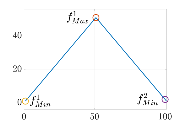
(a) piecewise strictly monotone signal

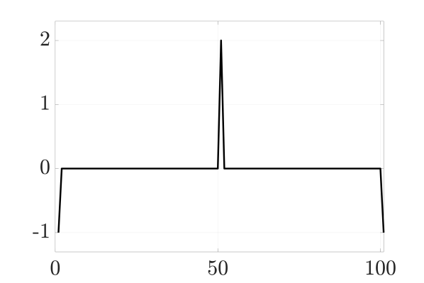
(b) A subgradient of the signal in (a)

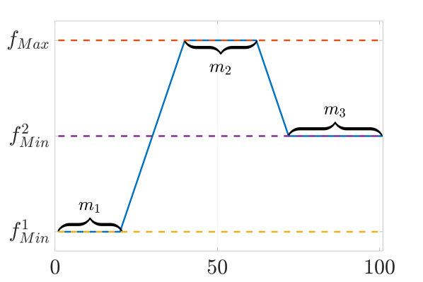
(c) piecewise monotone signal

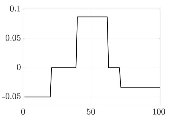
(d) A subgradient of the signal in (c)

Figure 1: Piecewise monotonic signals - (a) a piecewise monotone signal with one pixel at each extremum (b) its subgradient (c) a piecewise monotone signal (d) its subgradient.

Note that the subgradient depends on the relation between the pixels. Namely, the subgradient is valid as long as the number of pixels, $\{m_{i}\}_{i=1}^{N}$, and their respective extrema attribute (minimum or maximum) do not change.

3.1.2 Subgradient Updating

Let $\mathcal{T}=\{T_{i}\}_{i=0}^{L}$ be the time points at which the subgradient changes, where $T_{0}=0$, and $T_{L}$ is the extinction time. These time points are when the relation among the extrema points changes. Equivalently, when the number of pixels in the extrema changes. An intersection between two adjacent pixels or number of pixels are termed merging event. From Attributes 3 and 7 we can find these time points and compute the updated subgradient.

Merging event prediction: The discrete gradient approximation is $\nabla\psi^{(j)}:=\psi^{(j+1)}-\psi^{(j)}=0$, where $\psi^{(j)}$ is the entry $j$ of the vector $\psi$. Using Eq. (17), the very next merging event after $T_{i}$ can be calculated by

$$T_{i+1}=T_{i}+\min_{j\in\mathcal{J}^{*}}\{-\nabla\psi^{(j)}(T_{i})/\nabla p^{(j)}(\psi(T_{i}))\},$$ (23)

where

$$\mathcal{J}^{*}=\{j\,\,s.t.\,\,0<-\nabla\psi^{(j)}(T_{i})/\nabla p^{(j)}(\psi(T_{i}))<\infty\}.$$

Subgradient updating: According to Attribute 7, the merged entries evolve together at the same pace. In addition, the subgradient at other locations is unchanged Since the average of the subgradient is zero (Attribute 4), the subgradient of the merged entries is the average of the previous subgradient at these entries. Merging event prediction and subgradient updating are detailed below and concisely formalized in Algorithm 2.

Algorithm 2 Accelerated TV flow

1:Inputs:

2:      $f$

3:Initialize: $\psi_{0}\leftarrow f$, $t\leftarrow 0$, $\mathcal{T}=\emptyset$, and $\mathcal{P}=\emptyset$

4:Calculate the negative subgradient, $p_{0}$, of $f$ by invoking Algo. 1, add $p_{0}$ to the set $\mathcal{P}$.

5:while $\norm{p_{i}}>0$ do

6:     Find the next time transition point, $T_{i+1}$ (Eq. (23)).

7:     $\psi_{i+1}\leftarrow\psi_{i}+(T_{i+1}-T_{i})\cdot p_{i}$.

8:     Find clusters, $\{\mathcal{M}_{k}\}_{k=1}^{r}$, where $\absolutevalue{\nabla\psi_{i+1}}=0$

9:     Update the next negative subgradient, $p_{i+1}$, such that $p_{i+1}(\mathcal{M}_{k})=\frac{1}{\absolutevalue{\mathcal{M}_{k}}}\sum_{\mathcal{M}_{k}}p_{i}(\mathcal{M}_{k}),\quad k=1,\cdots,r.$

10:     Add $p_{i+1}$ to the set $\mathcal{P}$; Add $T_{i+1}$ to the set $\mathcal{T}$.

11:end while

12:Outputs: $\mathcal{T},\mathcal{P}$. The set $\mathcal{P}$ contains the negative subgradient sequence and the set $\mathcal{T}$ contains the transition times. Use Eq. (17) to get $\psi(t)$ for $t\in[0,T_{L}]$.

Remark 1 (TV flow - physical alegory)

For one dimensional signals, the TV flow initiates every pixel with an initial velocity. Then, the rest of the flow is a series of pure plastic collisions of the pixels. Thus, the velocity of the center of mass is preserved and equals zero.

3.1.3 Closed form solution

Let us assume an initial condition, $\psi(0)=f$, is orthogonal to the kernel of $J_{TV}$ (constant functions). The reconstruction of $f$ from the set of negative subgradients $\{p_{i}\}$ is burger2016spectral

$$,f=\psi(0)=\sum_{i=1}^{L}T_{i}(p_{i+1}-p_{i}).$$ (24)

Proposition 1 (Linear decay)

The solution of (TV-flow) is a sum of spectral components decaying linearly. More formally, if the initial condition, $f$, is orthogonal to the kernel set of $P$ then the solution of Eq. (TV-flow) is

$$\psi(t)=\sum_{i=1}^{L}\left(1+\lambda_{i}t\right)^{+}\varphi_{i},\,\,\textrm{where}\,\,\lambda_{i}=-T_{i}^{-1}\,\,\textrm{and}\,\,\varphi_{i}=\frac{p_{i}-p_{i+1}}{\lambda_{i}}.$$ (25)

Proof

Let us reformulate the solution, Eq. (17) for the first time range $t\in[0,T_{1}]$. Substituting Eq. (24) into Eq. (17), we have

$$\begin{split}\psi(t)&=\psi(0)+(t-0)p_{1}=\sum_{i=1}^{L}T_{i}(p_{i+1}-p_{i})+tp_{1}\\ &\quad\underbrace{=}_{p_{L+1}=0}\,\,\sum_{i=1}^{L}T_{i}(p_{i+1}-p_{i})+t\sum_{i=1}^{L}(p_{i}-p_{i+1})=\sum_{i=1}^{L}(T_{i}-t)(p_{i+1}-p_{i}).\end{split}$$

Therefore,

$$\psi(T_{1})=\sum_{i=1}^{L}(T_{i}-T_{1})(p_{i+1}-p_{i})=\sum_{i=2}^{L}(T_{i}-T_{1})(p_{i+1}-p_{i}).$$ (26)

In a similar manner, we can reformulate the solution for $t\in[T_{1},T_{2})$ as,

$$\psi(t)=\sum_{i=2}^{L}(T_{i}-t)(p_{i+1}-p_{i}).$$ (27)

By induction, the general solution is,

$$\psi(t)=\sum_{i=1}^{L}(T_{i}-t)^{+}(p_{i+1}-p_{i}).$$ (28)

Denoting $\lambda_{i}=-T_{i}^{-1}$, this can be expressed as,

$$\begin{split}\psi(t)&=\sum_{i=1}^{L}(-\lambda_{i}^{-1}-t)^{+}(p_{i+1}-p_{i})=\sum_{i=1}^{L}(1+\lambda_{i}t)^{+}\frac{p_{i}-p_{i+1}}{\lambda_{i}}.\quad\Box\end{split}$$

The spectral decomposition is computed by second order time derivative of $\psi(t)$ gilboa2014total ,

$$\mathcal{G}(t)=\sum_{i=1}^{L}\varphi_{i}\cdot t\lambda_{i}^{2}\cdot\delta(1+\lambda_{i}\cdot t).$$ (29)

This coincides with Attribute 5. A fast algorithm to find the TV spectral decomposition is proceeding Algo. 2. After finding the sets $\mathcal{P}$ and $\mathcal{T}$ we can calculate the spectral components $\{\varphi_{i}\}$ by Eq. (25).

The flow can also be defined (without using the operator $(\cdot)^{+}$) in disjoint time intervals,

$$\psi(t)=\sum_{i=k}^{L}\left(1+\lambda_{i}t\right)\varphi_{i},\quad\forall t\in[T_{k-1},T_{k}).$$ (30)

We will use this formulation later in our analysis.

3.2 Rescaled-DMD

We follow the work of cohen2020modes where an analysis of DMD was carried out for flows based on homogeneous operators. The homogeneity order dictates not only the decay profile but also the support in time of the solution. In particular, TV-flow decays linearly and has a finite extinction time. However, a flow linearization algorithm, such as DMD, can be interpreted as an exponential data fitting algorithm askham2018variable resulting in functions with infinite support. This contradiction yields an inherent error in the dynamic reconstruction by DMD. In cohen2020modes it was suggested to solve this problem by time reparameterization. Introducing a new time variable $\tau$, Eq. (TV-flow) is time rescaled by the flow,

$$\psi_{\tau}=G(\psi)=-\frac{\langle p,\psi\rangle}{\norm{p}^{2}}p\quad,-p\in\partial J_{TV}(\psi).$$ (R-TV-flow)

Note that, $G(a\psi)=aG(\psi),\,\forall a\in\mathbb{R}$, i.e. $G$ is a one-homogeneous operator. In addition, a TV eigenfunction is an eigenfunction of $G$, however, this eigenfunction decays exponentioally under the dynamics (R-TV-flow). Therefore, this flow rescales only the time axis whereas the spatial axis remains unchanged. Using (TV-flow) and (R-TV-flow), the relation between $t$ and $\tau$ can be derived by,

$$\begin{split}\frac{d}{d\tau}\psi(t(\tau))&=-\frac{\langle p,\psi(t(\tau))\rangle}{\norm{p}^{2}}p\\ &=-\frac{\langle p,\psi(t(\tau))\rangle}{\norm{p}^{2}}\frac{d}{dt}\psi(t(\tau)),\end{split}$$

yielding,

$$\frac{d}{d\tau}t(\tau)=-\frac{\langle p,\psi(t(\tau))\rangle}{\norm{p}^{2}}.$$ (31)

This ODE gets a different form in each segment, $[T_{k-1},T_{k})$. Substituting Eq. (30) in Eq. (31), we have

$$\frac{d}{d\tau}t(\tau)=-\frac{\langle\sum_{i=k}^{L}\lambda_{i}\varphi_{i},\sum_{i=k}^{L}\left(1+\lambda_{i}t(\tau)\right)\varphi_{i}\rangle}{\norm{\sum_{i=k}^{L}\lambda_{i}\varphi_{i}}^{2}}=-\frac{\sum_{i=k}^{L}\lambda_{i}\norm{\varphi_{i}}^{2}}{\sum_{i=k}^{L}\lambda_{i}^{2}\norm{\varphi_{i}}^{2}}-t(\tau).$$

The solution is,

$$t(\tau)=a_{k}e^{-\tau}-c_{k},\quad c_{k}=\frac{\sum_{i=k}^{L}\lambda_{i}\norm{\varphi_{i}}^{2}}{\sum_{i=k}^{L}\lambda_{i}^{2}\norm{\varphi_{i}}^{2}},$$ (32)

where $a_{k}$ depends on the initial conditions of every segment such that $t(\tau)$ is continuous (where $t(0)=0$). Then, the time points $\{T_{i}\}_{i=1}^{L}$ are mapped to $\{\tau_{i}\}_{i=1}^{L}$, accordingly.

Proposition 2 (Main TV-flow modes)

In every disjoint $k$th interval, $[\tau_{k-1},\tau_{k})$, the solution of time reparametrizing (TV-flow), Eq. (R-TV-flow), has two main orthogonal modes, $\xi_{1}^{k},\xi_{2}^{k}$, with eigenvalues zero and minus one.

Proof

Substituting Eq. (32) into Eq. (30), we get

$$\begin{split}\psi(t(\tau))&=\sum_{i=k}^{L}\left(1+\lambda_{i}t(\tau)\right)\varphi_{i},\qquad\qquad\qquad\forall t\in[T_{k-1},T_{k})\\ &=\sum_{i=k}^{L}\left(1+\lambda_{i}\left(a_{k}e^{-\tau}-c_{k}\right)\right)\varphi_{i},\qquad\qquad\forall\tau\in[\tau_{k-1},\tau_{k})\\ &=\underbrace{\sum_{i=k}^{L}\varphi_{i}-c_{k}\sum_{i=k}^{L}\lambda_{i}\varphi_{i}}_{\xi_{1}^{k}}+e^{-\tau}\underbrace{a_{k}\sum_{i=k}^{L}\lambda_{i}\varphi_{i}}_{\xi_{2}^{k}}=\xi_{1}^{k}+e^{-\tau}\xi_{2}^{k},\,\forall\tau\in[\tau_{k-1},\tau_{k}).\end{split}$$

By plugging $c_{k}$ from Eq. (32) into $\xi_{1}^{k},\xi_{2}^{k}$ their orthogonality is concluded immediately.$\quad\Box$

3.3 Analysis of the Rescaled-DMD

Here, we show a closed form solution to the time Rescaled-DMD (R-DMD). The common thread in the following discussion is Attribute 6, the orthogonality of the TV-spectral components. The method is summarized in Algorithm 3.

Theorem 3.1 (R-DMD of TV-flow)

Let $\tau_{0}$ be zero, then for the interval, $[\tau_{k-1},\tau_{k})$, where $k=1,\dots,L-1$, R-DMD reveals two non-zero orthogonal modes that reconstruct accurately the TV-flow in this interval. For the last interval, $[\tau_{L-1},\tau_{L})$, there is only one nonzero mode.

Proof

According to Prop. 2 and since DMD is an exponential data fitting algorithm, the DMD of the dynamics, Eq. (R-TV-flow), is as follows. The modes are $\phi_{1}^{k}={\xi_{1}^{k}}/{\norm{\xi_{1}^{k}}},\,\phi_{2}^{k}={\xi_{2}^{k}}/{\norm{\xi_{2}^{k}}}$, and the coefficients are $\alpha_{1}^{k}=\norm{\xi_{1}^{k}}$ and $\alpha_{2}^{k}=\norm{\xi_{2}^{k}}$. Note that one mode is constant with respect to time and the second decays exponentially. Therefore, the eigenvalues are $\mu_{1}^{k}=1$ for the constant mode and $\mu_{2}^{k}=e^{-dt}$ where $dt$ is the sampling step size (see Algo. 3). $\quad\Box$

Algorithm 3 R-DMD for TV-flow

1:Inputs: The initial condition $f$, and sampling step size $dt$.

2:Initialize: Evolve the solution of (R-TV-flow) uniformly with a step size $dt$.

3:Invoke Algo. 2 with the input $f$ - the result is $\mathcal{T}$ and $\mathcal{P}$.

4:Map the set of transition time points, $\mathcal{T}$, to a new set $\hat{\mathcal{T}}$ (Eq. (31)).

5:for Every time segment $[\tau_{i},\tau_{i+1}),\quad\tau_{i},\tau_{i+1}\in\hat{\mathcal{T}}$ do

6:     Invoke the classic DMD with $r=2$ (when $i=L-1$, $r=1$) schmid2010dynamic .

7:end for

8:Outputs: Modes $\{\phi_{1}^{k},\phi_{2}^{k}\}_{k=1}^{L}$, coefficients $\{\alpha_{1}^{k},\alpha_{2}^{k}\}_{k=1}^{L}$, and eigenvalues $\mu_{1}^{k}=1,\mu_{2}^{k}=e^{-dt}$.

Now we formulate the relation between the TV spectral components $\varphi_{k}$ and the R-DMD modes.

Proposition 3 (Revealing TV spectral components from R-DMD)

Given the result of Algo. 3, we can formulate the $k$th spectral component, $\varphi_{k}$, (Eq. (25)) by the following relation,

$$a_{k}\lambda_{k}\varphi_{k}=\alpha_{2}^{k}\phi_{2}^{k}-\frac{\langle\alpha_{2}^{k}\phi_{2}^{k},\alpha_{2}^{k+1}\phi_{2}^{k+1}\rangle}{\norm{\alpha_{2}^{k+1}\phi_{2}^{k+1}}^{2}}\alpha_{2}^{k+1}\phi_{2}^{k+1}.$$ (33)

Proof

$$\begin{split}\alpha_{2}^{k}\phi_{2}^{k}-&\frac{\langle\alpha_{2}^{k}\phi_{2}^{k},\alpha_{2}^{k+1}\phi_{2}^{k+1}\rangle}{\norm{\alpha_{2}^{k+1}\phi_{2}^{k+1}}^{2}}\alpha_{2}^{k+1}\phi_{2}^{k+1}=\xi_{2}^{k}-\frac{\langle\xi_{2}^{k},\xi_{2}^{k+1}\rangle}{\norm{\xi_{2}^{k+1}}^{2}}\xi_{2}^{k+1}=\\ &=a_{k}\sum_{i=k}^{L}\lambda_{i}\varphi_{i}-\frac{\langle a_{k}\sum_{i=k}^{L}\lambda_{i}\varphi_{i},a_{k+1}\sum_{i=k+1}^{L}\lambda_{i}\varphi_{i}\rangle}{\norm{a_{k+1}\sum_{i=k+1}^{L}\lambda_{i}\varphi_{i}}^{2}}a_{k+1}\sum_{i=k+1}^{L}\lambda_{i}\varphi_{i}\\ &=a_{k}\lambda_{k}\varphi_{k}+\\ &\qquad a_{k}\sum_{i=k+1}^{L}\lambda_{i}\varphi_{i}-a_{k}\frac{\langle\lambda_{k}\varphi_{k}+\sum_{i=k+1}^{L}\lambda_{i}\varphi_{i},\sum_{i=k+1}^{L}\lambda_{i}\varphi_{i}\rangle}{\norm{\sum_{i=k+1}^{L}\lambda_{i}\varphi_{i}}^{2}}\sum_{i=k+1}^{L}\lambda_{i}\varphi_{i}\\ &=a_{k}\lambda_{k}\varphi_{k}.\quad\Box\end{split}$$

3.4 Decay profile decomposition with Koopman modes of the TV flow

RDMD can be a solution for homogeneous flows when the dynamics belongs to $C^{1}$. However, it is limited when the dynamics is in $C^{0}$ almost everywhere cohen2021examining . The attribute of $C^{0}$ a.e. is equivalent to the fact that the Koopman modes do not exist during the entire dynamics.

Under the assumption that the dynamical system has a typical monotonic decay profile, a new method was suggested to find the Koopman modes cohen2021examining . We summarize this algorithm in Section 2.4. Now, we would like to apply this method on TV-flow. The typical decay profile of zero-homogeneous flows, such as TV-flow, is a linear function (see Eq. (25)) , and can be formulated as

$$a_{\lambda}(t)=(1+\lambda t)^{+}.$$ (34)

Denoting the step size as $dt$, we can formulate the dictionary, $D$, as

$$D=\begin{bmatrix}1&(1+\lambda_{1}dt)&\cdots\\ &\vdots&\\ 1&(1+\lambda_{N}dt)&\cdots\end{bmatrix}.$$ (35)

The goal is to find a sparse matrix $V$ such that

$$\Psi\approx VD.$$ (36)

4 A Two Dimensional Approximation of TV-flow

We now suggest a way to extend our fast algorithm (FGD) to two dimensions, approximating the anisotropic flow. Anisotropic TV plays an important role in mitigating edge sparsity required by many image processing applications, such as deconvolution, denoising, MRI construction lou2015weighted , and image segmentation bui2021weighted ; wu2021adaptive . There are previous approximations of 2D anisotropic TV minimizations, such as choksi2011anisotropic . However, there has been little research on fast TV-flow. Until now, a common practice is to solve a nonsmooth convex minimization problem at each time step (using Alternating Direction Method of Multipliers (ADMM), primal dual or other methods). This is very inefficient, naturally. Applying our proposed FGD algorithm can accelerate the process tremendously.

Anisotropic TV. The anisotropic TV is defined as follows,

$$J_{ani}(\psi)=\langle\norm{\nabla\psi}_{1},1\rangle=\langle\absolutevalue{D_{x}\psi}+\absolutevalue{D_{y}\psi},1\rangle.$$ (37)

We can calculate the subgradient of every column and row with Algo. 1. However, some of the properties of the 1D TV-flow are not valid in 2D. For example, the computation for the next merge event in a row is corrupted by the subgradient of a column. Therefore, we cannot update the subgradient with Algo. 2 and we should repeatedly compute the subgraident with Algo. 1.

Let $P^{(x)}$ be a matrix whose rows are the corresponding negative subgradients of the rows of $\psi$. Similarly, $P^{(y)}$ contains the negative subgradients of the columns of $\psi$. We assume that $P^{(x)}+P^{(y)}=0$ for every entry iff $P^{(x)}=0$ and $P^{(y)}=0$. Namely, it is most likely that the gradient descent flows of TV in $x$ and $y$ axes do not exactly cancel each other. The explicit scheme of the gradient descent flow is given by,

$$\psi_{k+1}=\psi_{k}+\left(P_{k}^{(x)}+P_{k}^{(y)}\right)dt_{k},\quad\psi_{0}=f,$$ (38)

where $P_{k}^{(x)}$ and $P_{k}^{(y)}$ denote the subgradients of $\psi_{k}$. The constraint on the step size $dt_{k}$ for which this explicit scheme converges is formulated in the following theorem.

Theorem 4.1 (Convergence of the explicit scheme)

Let us define the following ratio,

$$\tilde{\lambda}_{k}=\frac{\norm{P_{k}^{(x)}+P_{k}^{(y)}}^{2}}{J_{ani}(\psi_{k})},$$ (39)

where $J_{ani}(\psi_{k})$ is the anisotropic TV of $\psi_{k}$. For any time step $dt_{k}$ admitting,

$$dt_{k}=\frac{\delta}{\tilde{\lambda}_{k}},$$ (40)

where $\delta\in(0,2)$, the explicit scheme, Eq. (38), converges to steady state.

Proof

Let us examine the evolution of the $\ell^{2}$ norm of $\psi_{k}$ under the anisotopic TV-flow. We can formulate the norm of $\psi_{k+1}$ as

$$\begin{split}\norm{\psi_{k+1}}^{2}&=\norm{\psi_{k}+\left(P_{k}^{(x)}+P_{k}^{(y)}\right)dt_{k}}^{2}\\ &=\norm{\psi_{k}}^{2}+2\langle\psi_{k},P_{k}^{(x)}+P_{k}^{(y)}\rangle dt_{k}+\norm{\left(P_{k}^{(x)}+P_{k}^{(y)}\right)}^{2}\cdot dt_{k}^{2}\\ &=\norm{\psi_{k}}^{2}+2\langle\psi_{k},P_{k}^{(x)}+P_{k}^{(y)}\rangle\delta\frac{J_{ani}(\psi_{k})}{\norm{P_{k}^{(x)}+P_{k}^{(y)}}^{2}}\\ &\qquad+\norm{P_{k}^{(x)}+P_{k}^{(y)}}^{2}\cdot\delta^{2}\frac{J(\psi_{k})^{2}}{\norm{P_{k}^{(x)}+P_{k}^{(y)}}^{4}}\\ &=\norm{\psi_{k}}^{2}-2\delta\frac{J_{ani}(\psi_{k})^{2}}{\norm{P_{k}^{(x)}+P_{k}^{(y)}}^{2}}+\delta^{2}\frac{J_{ani}(\psi_{k})^{2}}{\norm{P_{k}^{(x)}+P_{k}^{(y)}}^{2}}\\ &=\norm{\psi_{k}}^{2}+\left(\delta^{2}-2\delta\right)\frac{J_{ani}(\psi_{k})^{2}}{\norm{P_{k}^{(x)}+P_{k}^{(y)}}^{2}}\end{split}$$ (41)

Since $\delta\in(0,2)$, $\norm{\psi_{k+1}}^{2}-\norm{\psi_{k}}^{2}\leq 0$. Then, the series $\{\norm{\psi_{k}}\}^{2}$ is monotonically decreasing and bounded from below by zero, therefore converges. Then, the difference between two successive elements converges to zero. Since the term $\delta^{2}-2\delta$ is constant then the ratio $\frac{J_{ani}(\psi_{k})^{2}}{\norm{P_{k}^{(x)}+P_{k}^{(y)}}^{2}}$ converges to zero. In addition, the denominator is bounded from above, therefore, $J(\psi_{k})\to 0$ as $k\to\infty$.

5 Results

In this section, we illustrate the theory and algorithms discussed above. We use standard first-order discretization of the derivatives and Neumann boundary conditions.

5.1 1D results

We begin with a toy example, depicted in Fig. 2(a). We show that the solution of (TV-flow) decays linearly (Fig. 2(b)) and that of Eq. (R-TV-flow) piecewise exponentially, (Fig. 2(c)).

(a) Toy example

(b) TV-flow $\psi(t)$

(c) R-TV-flow, $\psi(\tau)$

Figure 2: Time reparametrization - (a) The initial condition is a signal with three pulses with different widths. (b) TV-flow $\psi(t)$ decays piecewise linearly. (c) R-TV-flow, $\psi(t)$ is mapped to a piecewise smooth function. The non-smooth points represent transitions in the subgradient.

In Fig. 3 we show the TV-modes defined in Prop. 2 with the initial condition Fig. 2(a). It contains six disjoint intervals with the corresponding modes $\{\xi_{1}^{k},\xi_{2}^{k}\}_{k=1}^{6}$.

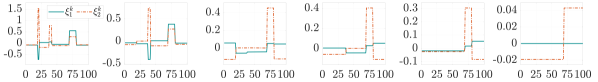
Figure 3: Modes: $\xi_{1}^{k}$ (teal) - constant, $\xi_{2}^{k}$ (orange) - exponentially decaying.

In Fig. 4-top the TV-spectral decomposition, dashed red line (computed in the standard way, see gilboa2014total ) is compared with two algorithms: Algorithm 3 based on Prop. 3, black dotted line, and Algorithm 2, blue line. The errors between the TV-spectral decomposition and Algorithms 3 and 2 are depicted in Fig. 4-bottom. We can observe an excellent match in both cases.

Figure 4: TV spectral decomposition comparison for toy example - The standard method of spectral decomposition (Dashed red line) vs. fast TV decomposition and R-DMD decomposition in blue and dotted black lines respectively. Bottom row - respecive errors

In Fig. 5, we show results of the fast TV-spectral decomposition, Algorithm 2, applied on a natural signal. We arbitrarily chose the red line from the zebra in Fig. 5(a), depicted in Fig. 5(b). Bands of standard TV-spectral decomposition and the fast TV-spectral decomposition are shown in Fig. 5(c). One can observe that our proposed fast method recovers the spectral bands faithfully, with negligible error, Fig. 5(d).

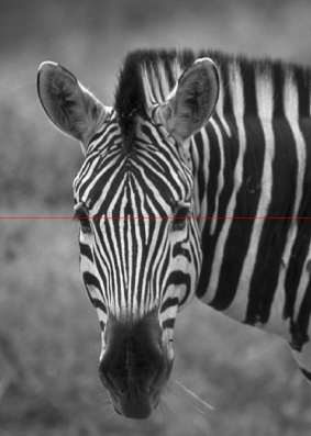
(a) Zebra image

(b) The red line from (a)

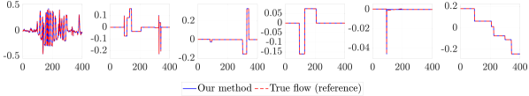
(c) TV-spectral decomposition

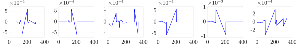
(d) Error

Figure 5: TV spectral decomposition comparison for an arbitrary initial condition - (b) The corresponding values of the pixels on the red line in (a). (c) Standard method of spectral decomposition (Dashed red line) vs. fast TV decomposition (Blue line). (d) The respective error.

Rough performance comparison. We report the elapsed time in seconds, running in Matlab 2018b on an 8th Gen. Core i7 laptop with 16GB RAM. Initial condition Fig. 2(a): Standard method (iterative application of chambolle2004algorithm ) - $488.4$s; ours - $0.013$s. Initial condition Fig. 5(b) (zebra): Standard method - $7.1\times 10^{3}$s; ours - $0.15$s.

5.2 2D results

Here we compare between isotropic and anisotropic TV-spectral decomposition and between the TV-spectral decomposition and the decay profile decomposition with Koopman modes (36). The Anisotropic TV-Flow is computed by the accelerated flow based on Theorem 4.1. The algorithm to approximate the Koopman mode is dictated by the typical decay profile and formulated in 3.4.

In Fig. 6(a), we show the isotropic TV spectral decomposition of the Zebra from Fig. 5(a). In Figs. 6(b)–6(e), we show the decomposition according to the percentage depicted in Fig. 6(a).

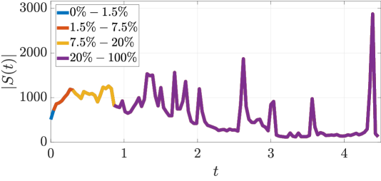
(a)

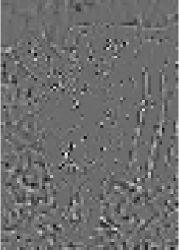
(b)

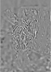
(c)

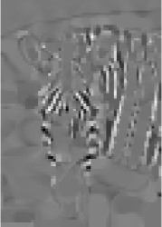
(d)

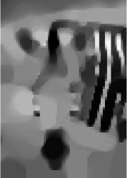
(e)

Figure 6: Zebra image isotropic TV-decomposition

In Fig. 7, we present the decomposition results to the same band separation, but this time based on Eq. (36). From a qualitative perspective, a very similar decomposition is obtained.

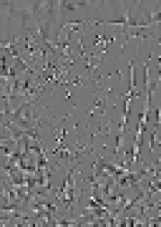
(a)

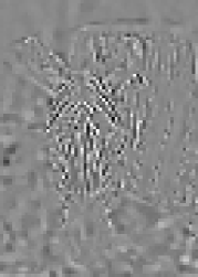
(b)

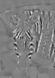
(c)

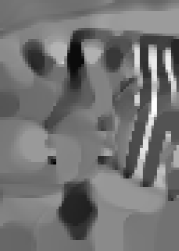
(d)

Figure 7: Zebra image - decay profile decomposition with Koopman modes of isotropic TV flow

In Fig. 8(a), the anisotropic TV-spectrum is presented and the decomposition according to the percentage in 8(a) is depicted in Figs. 8(b)–8(e).

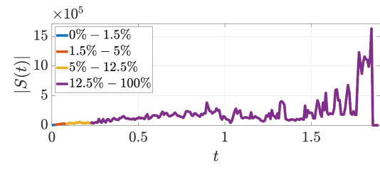
(a)

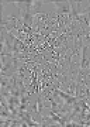
(b)

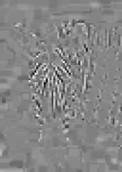
(c)

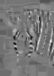
(d)

(e)

Figure 8: Zebra image anisotropic TV-decomposition, computed by the accelerated flow, Theorem 4.1 and Algo. 1.

We show the corresponding decay profile decomposition in Fig. 9

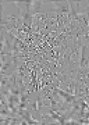
(a)

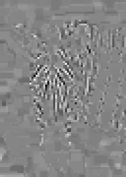
(b)

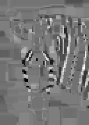
(c)

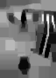
(d)

Figure 9: Zebra image - decay profile decomposition with Koopman modes of anisotropic TV flow, computed by the accelerated flow, Theorem 4.1 and Algo. 1.

6 Conclusion

In this paper we thoroughly examined the DMDschmid2010dynamic algorithm and Koopman Theory as tools for spectral analysis and decomposition of the TV-flow. We proposed the Rescaled Dynamic Mode Decomposition (RDMD) adaptation as a means to overcome difficulties in DMD application due to the linear-decay nature of the TV flow. We have found exact relations between TV spectral decomposition, the Koopman Mode Decomposition (KMD) algorithm and DMD. Due to the discontinuity of the dynamic, a decomposition based on the decay profile cohen2021examining is called for. We applied this decomposition to separate the flow into Koopman modes, to compare them against the original TV spectral decomposition.

Since evolving TV-flow is a slow process using optimization techniques, we have proposed a very fast method, based on simple updates of the subgradient. Finally, our accelerated algorithm was extended for solving the two-dimensional anisotropic TV-Flow.

Acknowledgements. This work was supported by the European Union’s Horizon 2020 research and innovation programme under the Marie Skłodowska-Curie grant agreement No. 777826 (NoMADS). GG acknowledges support by the Israel Science Foundation (Grant No. 534/19) and by the Ollendorff Minerva Center.

References

- (1) Andreu, F., Ballester, C., Caselles, V., Mazón, J.M.: Minimizing total variation flow. Differential and Integral Equations 14(3), 321–360 (2001)
- (2) Askham, T., Kutz, J.N.: Variable projection methods for an optimized dynamic mode decomposition. SIAM Journal on Appl. Dyn. Sys. 17(1), 380–416 (2018)
- (3) Bellettini, G., Caselles, V., Novaga, M.: The total variation flow in rn. Journal of Differential Equations 184(2), 475–525 (2002)
- (4) Bonforte, M., Figalli, A.: Total variation flow and sign fast diffusion in one dimension. Journal of Differential Equations 252(8), 4455–4480 (2012)
- (5) Brokman, J., Gilboa, G.: Nonlinear spectral processing of shapes via zero-homogeneous flows. In: A. Elmoataz, J. Fadili, Y. Quéau, J. Rabin, L. Simon (eds.) Scale Space and Variational Methods in Computer Vision, pp. 40–51. Springer International Publishing, Cham (2021)
- (6) Brox, T., Weickert, J.: A TV flow based local scale estimate and its application to texture discrimination. J. of Vis. Comm. and Image Rep. 17(5), 1053–1073 (2006)
- (7) Brox, T., Welk, M., Steidl, G., Weickert, J.: Equivalence results for tv diffusion and tv regularisation. In: International Conference on Scale-Space Theories in Computer Vision, pp. 86–100. Springer (2003)
- (8) Bui, K., Park, F., Lou, Y., Xin, J.: A weighted difference of anisotropic and isotropic total variation for relaxed mumford–shah color and multiphase image segmentation. SIAM Journal on Imaging Sciences 14(3), 1078–1113 (2021)
- (9) Bungert, L., Burger, M., Chambolle, A., Novaga, M.: Nonlinear spectral decompositions by gradient flows of one-homogeneous functionals. Analysis & PDE 14(3), 823–860 (2021)
- (10) Burger, M., Gilboa, G., Moeller, M., Eckardt, L., Cremers, D.: Spectral decompositions using one-homogeneous functionals. SIAM Im. Sci. 9(3), 1374–1408 (2016)
- (11) Chambolle, A.: An algorithm for total variation minimization and applications. Journal of Mathematical imaging and vision 20(1-2), 89–97 (2004)
- (12) Chambolle, A., Caselles, V., Cremers, D., Novaga, M., Pock, T.: An introduction to total variation for image analysis. Theoretical foundations and numerical methods for sparse recovery 9(263-340), 227 (2010)
- (13) Cherkaoui, H., Sulam, J., Moreau, T.: Learning to solve tv regularised problems with unrolled algorithms. Adv.Neural Inf. Proc. Sys. 33 (2020)
- (14) Choksi, R., van Gennip, Y., Oberman, A.: Anisotropic total variation regularized approximation and denoising/deblurring of 2d bar codes. Inverse Problems & Imaging 5(3), 591 (2011)
- (15) Cohen, I., Azencot, O., Lifshits, P., Gilboa, G.: Modes of homogeneous gradient flows. arXiv preprint arXiv:2007.01534 (2020)
- (16) Cohen, I., Berkov, T., Gilboa, G.: Total-variation mode decomposition. In: A. Elmoataz, J. Fadili, Y. Quéau, J. Rabin, L. Simon (eds.) Scale Space and Variational Methods in Computer Vision, pp. 52–64. Springer International Publishing, Cham (2021)
- (17) Cohen, I., Gilboa, G.: Introducing the p-laplacian spectra. Signal Processing 167, 107281 (2020)
- (18) Cohen, I., Gilboa, G.: Examining the limitations of dynamic mode decomposition through koopman theory analysis. arXiv preprint arXiv:2107.07456 (2021)
- (19) Darbon, J., Sigelle, M.: Image restoration with discrete constrained total variation part i: Fast and exact optimization. J. Math. Im. and Vision 26(3), 261–276 (2006)
- (20) Elmore, C.T., Dowling, A.W.: Learning spatiotemporal dynamics in wholesale energy markets with dynamic mode decomposition. Energy p. 121013 (2021)
- (21) Fumero, M., Möller, M., Rodolà, E.: Nonlinear spectral geometry processing via the tv transform. ACM Transactions on Graphics (TOG) 39(6), 1–16 (2020)
- (22) Gilboa, G.: A spectral approach to total variation. In: Inter. Conf. on Scale Space and Variational Methods in Computer Vision, pp. 36–47. Springer (2013)
- (23) Gilboa, G.: A total variation spectral framework for scale and texture analysis. SIAM journal on Imaging Sciences 7(4), 1937–1961 (2014)
- (24) Gilboa, G., Moeller, M., Burger, M.: Nonlinear spectral analysis via one-homogeneous functionals: Overview and future prospects. Journal of Mathematical Imaging and Vision 56(2), 300–319 (2016)
- (25) Goldfarb, D., Yin, W.: Parametric maximum flow algorithms for fast total variation minimization. SIAM J. Sci. Comp. 31(5), 3712–3743 (2009)
- (26) Koopman, B.O.: Hamiltonian systems and transformation in hilbert space. Proceedings of the national academy of sciences of the united states of america 17(5), 315 (1931)
- (27) Kuijper, A.: p-laplacian driven image processing. In: 2007 IEEE International Conference on Image Processing, vol. 5, pp. V–257. IEEE (2007)
- (28) Lou, Y., Zeng, T., Osher, S., Xin, J.: A weighted difference of anisotropic and isotropic total variation model for image processing. SIAM Journal on Imaging Sciences 8(3), 1798–1823 (2015)
- (29) Mezić, I.: Spectral properties of dynamical systems, model reduction and decompositions. Nonlinear Dynamics 41(1-3), 309–325 (2005)
- (30) Rosenfeld, J.A., Kamalapurkar, R.: Singular dynamic mode decompositions. arXiv preprint arXiv:2106.02639 (2021)
- (31) Schmid, P.J.: Dynamic mode decomposition of numerical and experimental data. Journal of fluid mechanics 656, 5–28 (2010)
- (32) Steidl, G., Didas, S., Neumann, J.: Relations between higher order TV regularization and support vector regression. In: Inter. Conf. on Scale-Space Theories in Computer Vision, pp. 515–527. Springer (2005)
- (33) Steidl, G., Weickert, J., Brox, T., Mrázek, P., Welk, M.: On the equivalence of soft wavelet shrinkage, total variation diffusion, total variation regularization, and sides. SIAM J. on Num. Ana. 42(2), 686–713 (2004)
- (34) Wu, T., Gu, X., Wang, Y., Zeng, T.: Adaptive total variation based image segmentation with semi-proximal alternating minimization. Signal Processing 183, 108017 (2021)
- (35) Zhang, H., Dawson, S.T., Rowley, C.W., Deem, E.A., Cattafesta, L.N.: Evaluating the accuracy of the dynamic mode decomposition. Journal of Computational Dynamics 7(1), 35–56 (2020)