Computing the Fréchet Distance Between Uncertain Curves in One Dimension

Abstract

We consider the problem of computing the Fréchet distance between two curves for which the exact locations of the vertices are unknown. Each vertex may be placed in a given uncertainty region for that vertex, and the objective is to place vertices so as to minimise the Fréchet distance. This problem was recently shown to be NP-hard in 2D, and it is unclear how to compute an optimal vertex placement at all.

We present the first general algorithmic framework for this problem. We prove that it results in a polynomial-time algorithm for curves in 1D with intervals as uncertainty regions. In contrast, we show that the problem is NP-hard in 1D in the case that vertices are placed to maximise the Fréchet distance.

We also study the weak Fréchet distance between uncertain curves. While finding the optimal placement of vertices seems more difficult than the regular Fréchet distance – and indeed we can easily prove that the problem is NP-hard in 2D – the optimal placement of vertices in 1D can be computed in polynomial time. Finally, we investigate the discrete weak Fréchet distance, for which, somewhat surprisingly, the problem is NP-hard already in 1D.

1 Introduction

The Fréchet distance is a popular distance measure for curves. Its computational complexity has drawn considerable attention in computational geometry [2, 5, 7, 8, 11, 17, 21]. The Fréchet distance between two (polygonal) curves is often illustrated using a person and a dog: imagine a person is walking along one curve having the dog, which walks on the other curve, on a leash. The person and the dog may change their speed independently but may not walk backwards. The Fréchet distance corresponds to the minimum leash length needed with which the person and the dog can walk from start to end on their respective curve.

The Fréchet distance and its variants have found many applications, for instance, in the context of protein alignment [22], handwriting recognition [29], map matching [6] and construction [3, 9], and trajectory similarity and clustering [12, 20]. In most of these applications, we obtain the curves by a sequence of measurements, and these measurements are inherently imprecise. However, it is often reasonable to assume that the true location is within a certain radius of the measurement, or more generally that it stays within an uncertainty region.

Re-imagine the person and the dog, except now each is given a sequence of regions they have to visit. More specifically, they need to visit one location per region and move on a straight line between locations without going backwards. Suppose they need to minimise the leash length. This corresponds to the following problem. Each curve is given by a sequence of uncertainty regions; we minimise the Fréchet distance over all possible choices of locations in the regions. This is called the lower bound problem for the Fréchet distance between uncertain curves.

Similar problems involving uncertainty have drawn more and more attention in the past few years in computational geometry. Most results are on uncertain point sets, where we often aim to minimise or maximise some quantity stemming from the point set, but also perform visibility queries in polygons or find Delaunay triangulations [1, 14, 18, 23, 24, 25, 26, 27, 28]. More recently there have also been several results on curves with uncertainty [4, 13, 16, 19].

The earliest results for a variant of the problem we consider do not concern the Fréchet distance as such, but its variant the discrete Fréchet distance, where we restrict our attention to the vertices of the curves. Ahn et al. [4] show a polynomial-time algorithm that decides whether the lower bound discrete Fréchet distance is below a certain threshold, for two curves with uncertainty regions modelled as circles in constant dimension. The lower bound Fréchet distance with uncertainty regions modelled as point sets admits a simple dynamic program [13]. However, as has been recently shown, the decision problem for the continuous Fréchet distance is NP-hard already in two dimensions with vertical line segments as uncertainty regions and one precise and one uncertain curve [13]; it is not even clear how to compute the lower bound at all with any uncertainty model that is not discrete. We present a general algorithmic framework for computing the lower bound Fréchet distance that can be instantiated in many settings. In the general 2D setting, this gives an exponential-time algorithm; we turn our attention to curves in 1D. We instantiate our framework in 1D and show that it results in an efficient algorithm for imprecision modelled as intervals.

Next to the discrete Fréchet distance, the most common variant of the Fréchet distance is the weak Fréchet distance [5]. In the person–dog analogy, this variant allows backtracking on the paths. The weak Fréchet distance (for certain curves) has interesting properties in 1D [10, 15, 21]: it can be computed in linear time in 1D, while in 2D it cannot be computed significantly faster than quadratic time under the strong exponential-time hypothesis. To our knowledge, the weak Fréchet distance has not been studied in the uncertain setting before. We give a polynomial-time algorithm that solves the lower bound problem in 1D. In contrast to that, we show that the problem is NP-hard in 2D, and that discrete weak Fréchet distance is NP-hard already in 1D. We summarise these results in Table 1.

Table 1: Complexity results for the lower bound problems for uncertain curves.

	Fréchet distance		Weak Fréchet distance
	discrete	continuous	discrete	continuous
1D	polynomial [4]	polynomial	NP-hard	polynomial
2D	polynomial [4]	NP-hard [13]	NP-hard	NP-hard

The table provides an interesting insight. First of all, it appears that for continuous distances the dimension matters, whereas for the discrete ones the results are the same both in 1D and 2D. Moreover, it may be surprising that discretising the problem has a different effect: for the Fréchet distance it makes it easier, while for the weak Fréchet distance the problem becomes harder. We discuss the polynomial-time algorithm for Fréchet distance in 1D in Section 4. We give the algorithm for weak Fréchet distance in 1D in Section 6.1. We show the NP-hardness constructions for the weak (discrete) Fréchet distance in Section 6.2.

Finally, we also turn our attention to the problem of maximising the Fréchet distance, or finding the upper bound. It has been shown that the problem is NP-hard in 2D for several uncertainty models, including discrete point sets, both for discrete and continuous Fréchet distance [13]. We strengthen that result by presenting a similar construction that already shows NP-hardness in 1D. The proof is given in Section 5.

2 Preliminaries

Denote $[n]\equiv\{1,2,\dots,n\}$. Consider a sequence of points $\pi=\langle p_{1},p_{2},\dots,p_{n}\rangle$. We also use $\pi$ to denote a polygonal curve, defined by the sequence by linearly interpolating between the points and can be seen as a continuous function: $\pi(i+\alpha)=(1-\alpha)p_{i}+\alpha p_{i+1}$ for $i\in[n-1]$ and $\alpha\in[0,1]$. The length of such a curve is the number of its vertices, $\lvert\pi\rvert=n$. Denote the concatenation of two sequences $\pi$ and $\sigma$ of lengths $n$ and $m$ by $\pi\sqcup\sigma$: the result consists of $\pi$, then $\sigma$. We can generalise this notation:

$$\pi\equiv\bigsqcup_{i\in[n]}p_{i}=p_{1}\sqcup p_{2}\sqcup\dots\sqcup p_{n}\,.$$

Denote a subcurve from vertex $i$ to $j$ of $\pi$ as $\pi[i:j]=p_{i}\sqcup p_{i+1}\sqcup\dots\sqcup p_{j}$. Occasionally we use the notation $\langle\pi(i)\mid i\in I\rangle_{i=1}^{m}$ to denote a curve built on a subsequence of vertices of $\pi$, where vertices are only taken if they are in set $I$. For example, setting $I=\{1,3,4\}$, $m=5$, $\pi=\langle p_{1},p_{2},\dots,p_{5}\rangle$ means $\langle\pi(i)\mid i\in I\rangle_{i=1}^{m}=\langle p_{1},p_{3},p_{4}\rangle$.

Denote the Fréchet distance between two polygonal curves $\pi$ and $\sigma$ by $d_{\mathrm{F}}(\pi,\sigma)$, the discrete Fréchet distance by $d_{\mathrm{dF}}(\pi,\sigma)$, and the weak Fréchet distance by $d_{\mathrm{wF}}(\pi,\sigma)$. Recall the definition of Fréchet distance for polygonal curves of lengths $m$ and $n$. It is based on parametrisations (non-decreasing surjections) $\alpha$ and $\beta$ with $\alpha\colon[0,1]\to[1,m]$, $\beta\colon[0,1]\to[1,n]$. Parametrisations establish a matching. Denote the cost of a matching $\mu=(\alpha,\beta)$ as $\mathrm{cost}_{\mu}(\pi,\sigma)=\max_{t\in[0,1]}\lVert\pi\circ\alpha(t)-\sigma\circ\beta(t)\rVert$. Then we can define Fréchet distance and its variants as

$$d_{\mathrm{F}}(\pi,\sigma)=\inf_{\text{matching }\mu}\mathrm{cost}_{\mu}(\pi,\sigma)\,,\quad d_{\mathrm{F}}(\pi,\sigma)=\inf_{\text{discrete matching }\mu}\mathrm{cost}_{\mu}(\pi,\sigma)\,,$$

$$d_{\mathrm{wF}}(\pi,\sigma)=\inf_{\text{weak matching }\mu}\mathrm{cost}_{\mu}(\pi,\sigma)\,.$$

The discrete matching is restricted to vertices, and the weak matching is not a pair of parametrisations, but a path $(\alpha,\beta)\colon[0,1]^{2}\to[1,m]\times[1,n]$, with $\alpha(0)=1,\alpha(1)=m$ and $\beta(0)=1,\beta(1)=n$. In the person–dog analogy for the Fréchet distance, the best choice of parametrisations means that the person and the dog choose the best speed, and the leash length is then the largest needed leash length during the walk.

An uncertain point in one dimension is a set of real numbers $u\subseteq\mathbb{R}$. The intuition is that only one point from this set represents the true location of the point; however, we do not know which one. A realisation $p$ of such a point is one of the points from $u$. In this paper we consider two special cases of uncertain points. An indecisive point is a finite set of numbers $u=\{x_{1},\dots,x_{\ell}\}$. An imprecise point is a closed interval $u=[x_{1},x_{2}]$. Note that a precise point is a special case of both indecisive and imprecise points.

Define an uncertain curve as a sequence of uncertain points $\mathcal{U}=\langle u_{1},\dots,u_{n}\rangle$. A realisation $\pi\Subset\mathcal{U}$ of an uncertain curve is a polygonal curve $\pi=\langle p_{1},\dots,p_{n}\rangle$, where each $p_{i}$ is a realisation of the uncertain point $u_{i}$. For uncertain curves $\mathcal{U}$ and $\mathcal{V}$, define the lower bound and upper bound Fréchet distance. The discrete and weak Fréchet distance are defined similarly.

$$d_{\mathrm{F}}^{\,\min}(\mathcal{U},\mathcal{V})=\min_{\pi\Subset\mathcal{U},\sigma\Subset\mathcal{V}}d_{\mathrm{F}}(\pi,\sigma)\,,\qquad d_{\mathrm{F}}^{\,\max}(\mathcal{U},\mathcal{V})=\max_{\pi\Subset\mathcal{U},\sigma\Subset\mathcal{V}}d_{\mathrm{F}}(\pi,\sigma)\,.$$

3 Lower Bound Fréchet Distance: General Approach

In this section, we consider the following decision problem.

Problem .

Given two uncertain curves $\mathcal{U}=\langle u_{1},\dots,u_{m}\rangle$ and $\mathcal{V}=\langle v_{1},\dots,v_{n}\rangle$ in $Y=\mathbb{R}^{d}$ for some $d,m,n\in\mathbb{N}^{+}$ and a threshold $\delta>0$, decide if $d_{\mathrm{F}}^{\,\min}(\mathcal{U},\mathcal{V})\leq\delta$.

Note that this problem formulation is general both in terms of the shape of uncertainty regions and the dimension of the problem. We propose an algorithmic framework that solves this problem. As has been shown previously [13], the problem is NP-hard in 2D for vertical line segments as uncertainty regions, but admits a simple dynamic program for indecisive points in 2D. So, in many uncertainty models, especially in higher dimensions, the following approach will not result in an efficient algorithm. However, our approach is general in that it can be instantiated in restricted settings, e.g. in 2D assuming that the segments of the curves can only be horizontal or vertical. The inherent complexity of the problem appears to be related to the number of directions to consider, with the infinite number in 2D without restrictions and two directions in 1D). We conjecture that in this restricted setting the approach yields a polynomial-time algorithm; verifying this and making a more general statement delineating the hardness of restricted settings are both interesting open problems. Our approach shows a straightforward way to engineer an algorithm for various restricted settings in arbitrary dimension, but we cannot make any statements about its efficiency in most settings. To illustrate the approach, we instantiate it in 1D and analyse its efficiency in Section 4. The interested reader might refer to that section for a more intuitive explanation of the approach.

First we introduce some extra notation. For $i\in[m]$, denote $\mathcal{U}_{i}=\langle u_{1},\dots,u_{i}\rangle$ and $\mathcal{U}_{i}^{*}=\langle u_{1},\dots,u_{i},Y\rangle$. We call $\mathcal{U}_{i}$ and $\mathcal{U}_{i}^{*}$ the subcurve and the free subcurve of $\mathcal{U}$ at $i$, respectively. Intuitively, a realisation of $\mathcal{U}_{i}^{*}$ extends a realisation of $\mathcal{U}_{i}$ by a single edge whose final vertex position is unrestricted. Let $S:=S^{d-1}$ be the unit $(d-1)$-sphere. Denote the direction of the $i$-th edge $\pi[i,i+1]$ of a realisation $\pi$ by $\mathbf{d}_{i}(\pi)\subseteq S$. For example, in 1D there are only two options, in 2D the directions can be picked from a unit circle, in 3D from a unit sphere, etc. In the degenerate case where the edge has length $0$ (or $\pi$ has no $i$-th edge), let $\mathbf{d}_{i}(\pi)=S$.

We want to find realisations $\pi\Subset\mathcal{U}$ and $\sigma\Subset\mathcal{V}$ such that $\pi$ and $\sigma$ have Fréchet distance at most $\delta$. Call such a pair $(\pi,\sigma)$ a $\delta$-realisation of $(\mathcal{U},\mathcal{V})$. Recall that two polygonal curves $\pi\colon[1,i]\to Y$ and $\sigma\colon[1,j]\to Y$ have Fréchet distance $d_{\mathrm{F}}(\pi,\sigma)$ at most $\delta$ if and only if there exist parametrisations (non-decreasing surjections) $\alpha\colon[0,1]\to[1,i]$ and $\beta\colon[0,1]\to[1,j]$ such that the path $(\pi\circ\alpha,\sigma\circ\beta)$ lies in the $\delta$-free space $\mathcal{F}_{\delta}=\{(p,q)\in Y\times Y\mid\lVert p-q\rVert\leq\delta\}$. For $\delta$-close (free) subcurves of $\mathcal{U}$ at $i$ and $\mathcal{V}$ at $j$, we capture their pairs of endpoints and final directions using $\mathcal{R}_{i,j},\mathcal{R}_{i,j^{*}},\mathcal{R}_{i^{*},j},\mathcal{R}_{i^{*},j^{*}}\subseteq Y\times Y\times S\times S$:

$$\mathcal{R}_{i,j} =\{(\pi(i)\hphantom{{}\mathbin{+}1},\sigma(j)\hphantom{{}\mathbin{+}1},s,t)\mid\pi\Subset\mathmakebox[width("$\mathcal{U}_{i}^{*}$")]{\mathcal{U}_{i}},\sigma\Subset\mathmakebox[width("$\mathcal{V}_{j}^{*}$")]{\mathcal{V}_{j}},s\in\mathbf{d}_{i}(\pi),t\in\mathbf{d}_{j}(\sigma),d_{\mathrm{F}}(\pi,\sigma)\leq\delta\},$$

$$\mathcal{R}_{i,j^{*}} =\{(\pi(i)\hphantom{{}\mathbin{+}1},\sigma(j+1),s,t)\mid\pi\Subset\mathmakebox[width("$\mathcal{U}_{i}^{*}$")]{\mathcal{U}_{i}},\sigma\Subset\mathcal{V}_{j}^{*},s\in\mathbf{d}_{i}(\pi),t\in\mathbf{d}_{j}(\sigma),d_{\mathrm{F}}(\pi,\sigma)\leq\delta\},$$

$$\mathcal{R}_{i^{*},j} =\{(\pi(i+1),\sigma(j)\hphantom{{}\mathbin{+}1},s,t)\mid\pi\Subset\mathcal{U}_{i}^{*},\sigma\Subset\mathmakebox[width("$\mathcal{V}_{j}^{*}$")]{\mathcal{V}_{j}},s\in\mathbf{d}_{i}(\pi),t\in\mathbf{d}_{j}(\sigma),d_{\mathrm{F}}(\pi,\sigma)\leq\delta\},$$

$$\mathcal{R}_{i^{*},j^{*}} =\{(\pi(i+1),\sigma(j+1),s,t)\mid\pi\Subset\mathcal{U}_{i}^{*},\sigma\Subset\mathcal{V}_{j}^{*},s\in\mathbf{d}_{i}(\pi),t\in\mathbf{d}_{j}(\sigma),d_{\mathrm{F}}(\pi,\sigma)\leq\delta\}.$$

Note that for $\pi\Subset\mathcal{U}_{i}$, $i$ is the final vertex, so $\mathbf{d}_{i}(\pi)=S$. Therefore, $\mathcal{R}_{i,j}$ captures the reachable subset of $Y\times Y$ for the realisations of the last points of the prefixes, and the two other dimensions contain all points from $S$ to capture that we may proceed in any allowed direction. The set $\mathcal{R}_{i^{*},j}$ captures the reachable subset of $Y\times Y$ for the point in the parametrisation where we are between vertices $i$ and $i+1$ on $\mathcal{U}$ and at $j$ on $\mathcal{V}$; we have not restricted the range to $u_{i+1}$ yet. The allowed directions for parameter $s$ now depend on how we reached this point in the parametrisation, since segments connecting realisations are straight line segments, and the direction needs to be kept consistent once chosen. From this description the reader can deduce what the other sets capture by symmetry. See also Figure 1, where the sets are positioned as in a regular free-space diagram, replacing the edges, vertices, and cells.

(a) The sets on a cell of a regular free-space diagram.

(b) Dependencies of the dynamic program. $a\to b$ means that $a$ depends on $b$.

Figure 1: Illustration for the dynamic program of Lemma 3.1.

To solve the decision problem, we must decide whether $\mathcal{R}_{m,n}$ is non-empty. If so, then there are realisations of $\mathcal{U}_{m}\equiv\mathcal{U}$ and $\mathcal{V}_{n}\equiv\mathcal{V}$ that are close enough in terms of the Fréchet distance. We compute $\mathcal{R}_{\cdot,\cdot}$ using dynamic programming. We illustrate the propagation dependencies in Figure 1 and make them explicit in Lemma 3.1.

Lemma 3.1.

Let $\star(A):=\{(p+\lambda s,q+\mu t,s,t)\mid(p,q,s,t)\in A\text{ and }\lambda,\mu\geq 0\}$. We have

$$\mathcal{R}_{\cdot,0}=\mathcal{R}_{0,\cdot} =\emptyset\,,$$

$$\mathcal{R}_{i+1,j^{*}} =\{(p,q,s,t)\in u_{i+1}\times\mathmakebox[width("$v_{j+1}$")]{Y}\times S\times S\mid(p,q,\mathmakebox[width("$s$")]{\cdot},t)\in\mathcal{R}_{i^{*},j^{*}}\}\,,$$

$$\mathcal{R}_{i^{*},j+1} =\{(p,q,s,t)\in\mathmakebox[width("$u_{i+1}$")]{Y}\times v_{j+1}\times S\times S\mid(p,q,s,\mathmakebox[width("$t$")]{\cdot})\in\mathcal{R}_{i^{*},j^{*}}\}\,,$$

$$\mathcal{R}_{i+1,j+1} =\{(p,q,s,t)\in u_{i+1}\times v_{j+1}\times S\times S\mid(p,q,\mathmakebox[width("$s$")]{\cdot},\mathmakebox[width("$t$")]{\cdot})\in\mathcal{R}_{i^{*},j^{*}}\}\,,$$

$$\mathcal{R}_{0^{*},0^{*}} =\mathcal{F}_{\delta}\times S\times S\,,$$

$$\mathcal{R}_{i^{*},j^{*}} =(\mathcal{F}_{\delta}\times S\times S)\cap\star(\mathcal{R}_{i,j}\cup\mathcal{R}_{i^{*},j}\cup\mathcal{R}_{i,j^{*}})\quad\text{for $i>0$ or $j>0$.}$$

Proof 3.2.

The first equation holds because the empty function has no parametrisation, so the Fréchet distance of any pair of realisations is infinite. The equation for $\mathcal{R}_{i+1,j^{*}}$ holds because for $\pi\Subset\mathcal{U}_{i+1}$, $\mathbf{d}_{i+1}(\pi)=S$, and the only additional constraint that a realisation of $\mathcal{U}_{i+1}$ has over one of $\mathcal{U}_{i}^{*}$ is that the final vertex lies in $u_{i+1}$. Using symmetric properties on $\mathcal{V}$, we obtain the equations for $\mathcal{R}_{i^{*},j+1}$ and $\mathcal{R}_{i+1,j+1}$. The equation for $\mathcal{R}_{0^{*},0^{*}}$ concerns curves $\pi$ and $\sigma$ consisting of a single vertex, so $\mathbf{d}_{0}(\pi)=\mathbf{d}_{0}(\sigma)=S$, and $d_{\mathrm{F}}(\pi,\sigma)\leq\delta$ if and only if $(\pi(1),\sigma(1))\in\mathcal{F}_{\delta}$. The equation for $\mathcal{R}_{i^{*},j^{*}}$ remains. First we show that the right-hand side is contained in $\mathcal{R}_{i^{*},j^{*}}$. Suppose that $\pi$ and $\sigma$ form a witness for $(p,q,s,t)\in\mathcal{R}_{i,j}\cup\mathcal{R}_{i^{*},j}\cup\mathcal{R}_{i,j^{*}}$. We obtain realisations $\pi^{*}\Subset\mathcal{U}_{i}^{*}$ and $\sigma^{*}\Subset\mathcal{V}_{j}^{*}$ by extending the last edge of $\pi$ and $\sigma$ in the direction it is already going (or adding a new edge in an arbitrary direction if $\pi\Subset\mathcal{U}_{i}$ or $\sigma\Subset\mathcal{V}_{j}$), to $(p+\lambda s,q+\mu t)$. If $(p+\lambda s,q+\mu t)\in\mathcal{F}_{\delta}$, then, by convexity of $\mathcal{F}_{\delta}$, the extensions of the last edges have Fréchet distance at most $\delta$ (since the points at which the extension starts have distance at most $\delta$), so $(p+\lambda s,q+\mu t,s,t)\in\mathcal{R}_{i^{*},j^{*}}$. Conversely, we show that the right-hand side contains $\mathcal{R}_{i^{*},j^{*}}$. Let $\pi^{*}\Subset\mathcal{U}_{i}^{*}$ and $\sigma^{*}\Subset\mathcal{V}_{j}^{*}$ together with parametrisations $\alpha\colon[0,1]\to[1,i+1]$ and $\beta\colon[0,1]\to[1,j+1]$ form a witness that $(p,q,s,t)\in\mathcal{R}_{i^{*},j^{*}}$. Then, for any $x\in[0,1]$, the restrictions $\pi_{x}$ of $\pi^{*}$ and $\sigma_{x}$ of $\sigma^{*}$ to the domains $[1,\alpha(x)]$ and $[1,\beta(x)]$ have Fréchet distance at most $\delta$. Because $\alpha$ and $\beta$ are non-decreasing surjections, whenever $i>0$ or $j>0$, there exists some $x$ such that

1. $\alpha(x)=i$ and $\beta(x)=j$, in which case $\pi_{x}\Subset\mathcal{U}_{i}$ and $\sigma_{x}\Subset\mathcal{V}_{j}$, or

2. $\alpha(x)>i$ and $\beta(x)=j$, in which case $\pi_{x}\Subset\mathcal{U}_{i}^{*}$ and $\sigma_{x}\Subset\mathcal{V}_{j}$, or

3. $\alpha(x)=i$ and $\beta(x)>j$, in which case $\pi_{x}\Subset\mathcal{U}_{i}$ and $\sigma_{x}\Subset\mathcal{V}_{j}^{*}$.

Note that if $i=0$, only the second case applies, and if $j=0$, only the third case applies. In each case, the last edge of $\pi^{*}$ and $\sigma^{*}$ extends the $i$-th and $j$-th edge of $\pi_{x}$ and $\sigma_{x}$, respectively. So $(\pi_{x},\sigma_{x})$ forms a witness that $(p,q,s,t)$ is contained in the right-hand side.

Simplifying the approach.

Due to their dimension, the above sets can be impractical to work with. However, for the majority of these sets, at least one of the factors $S$ carries no additional information, as formulated below. Denote by $\mathrm{Pr}_{c}$ the projection map of the $c$-th component, so that $\mathrm{Pr}_{1}\colon(p,q,s,t)\mapsto p$, and in general $\mathrm{Pr}_{c_{1},\dots,c_{k}}(x)=(\mathrm{Pr}_{c_{1}}(x),\dots,\mathrm{Pr}_{c_{k}}(x))$. The equations of Lemma 3.1 imply the equivalences

$$(p,q,s,t)\in\mathcal{R}_{i,j\hphantom{{}^{*}}} \iff\hphantom{\leavevmode\nobreak\ t,}(p,q)\in\mathrm{Pr}_{1,2}(\mathcal{R}_{i,j})\,,$$

$$(p,q,s,t)\in\mathcal{R}_{i^{*},j} \iff(p,q,s)\in\mathrm{Pr}_{1,2,3}(\mathcal{R}_{i^{*},j})\,,$$

$$(p,q,s,t)\in\mathcal{R}_{i,j^{*}} \iff(p,q,t)\in\mathrm{Pr}_{1,2,4}(\mathcal{R}_{i,j^{*}})\,.$$

Consequently, to find $\mathcal{R}_{i,j}$, $\mathcal{R}_{i^{*},j}$, and $\mathcal{R}_{i,j^{*}}$, it suffices to compute the projections above. This simplifies the prior dependencies as shown in Figure 2.

$$\mathrm{Pr}_{1,2}(\mathcal{R}_{i+1,j+1}) =(u_{i+1}\times v_{j+1})\cap\mathrm{Pr}_{1,2}(\mathcal{R}_{i^{*},j^{*}})$$

$$=(u_{i+1}\times\mathmakebox[width("$v_{j+1}$")]{Y})\cap\mathrm{Pr}_{1,2}(\mathcal{R}_{i^{*},j+1})$$

$$=(\mathmakebox[width("$u_{i+1}$")]{Y}\times v_{j+1})\cap\mathrm{Pr}_{1,2}(\mathcal{R}_{i+1,j^{*}})\,.$$

Figure 2: Simplified dependencies with projections as follows from Lemma 3.1.

Instantiating the approach.

The dynamic program of Lemma 3.1 can naturally be adapted to constrained realisations whose edge directions are to be drawn from a subset $S^{\prime}\subseteq S^{d-1}$, by replacing $S$ by $S^{\prime}$, so the framework can be used for restricted settings in 2D. For $S=S^{d-1}$ the complexity of $R_{i,j}$ can be exponential, so it can be useful to restrict the problem.

We can look at the construction used to prove NP-hardness of the problem in 2D [13] as an example for our approach. There the curve $\mathcal{V}$ is precise, so each $v_{j}$ is a single point and each $t$ is predetermined, and curve $\mathcal{U}$ consists of uncertainty regions that are vertical line segments, so each $u_{i}$ has a fixed $x$-coordinate and a range of $y$-coordinates. If we now exclude the fixed values from our propagation, we get to track pairs $(y,s)$ of the feasible $y$-coordinates on the current interval and the directions. We start with a single region. The hardness construction uses gadgets on the precise curve to force the uncertain curve to go through certain points. In our approach, this means that we keep restricting the set of feasible directions while passing by vertices on $\mathcal{V}$, and eventually each point in the starting region gives rise to two disjoint reachable points on one of the following uncertainty regions. So we can use our algorithm to correctly track the feasible $y$-coordinates through the construction; however, we would need to keep track of regions of exponential complexity, which is, predictably, inefficient. Therefore, it is important to analyse the complexity of the propagated regions to determine whether our approach gives rise to an efficient algorithm. To illustrate our approach, we use it in the 1D case to devise an efficient algorithm in Section 4.

4 Lower Bound Fréchet Distance: One Dimension

In this section we instantiate the approach of Section 3 in 1D and analyse its efficiency. We first show the formal definitions that result from this process, and then give some intuition for how the resulting algorithm works in 1D.

In our case, $S=S^{0}$, so there are only two directions: positive $x$-direction and negative $x$-direction. We make use of the projections interpretation and split the projections into two regions based on the value of the relevant direction; then all the regions we maintain are in $\mathbb{R}^{2}$ and have a geometric interpretation as feasible combinations of realisations of the last uncertain points on the prefixes of the curves. We omit $\mathcal{R}_{i,j}$ from our computations except for checking whether $\mathcal{R}_{m,n}$ is non-empty. As follows from the definition of the sets, $\mathcal{R}_{i,j}\subseteq\mathcal{R}_{i^{*},j}$ and $\mathcal{R}_{i,j}\subseteq\mathcal{R}_{i,j^{*}}$, so we can simplify the computation of $\mathcal{R}_{i^{*},j^{*}}$, and then we do not need the explicit computation of $\mathcal{R}_{i,j}$. Furthermore, we do not compute any of $\mathcal{R}_{i^{*},j^{*}}$ explicitly, opting instead to substitute them into the relevant expressions. Therefore, we maintain the sets $\mathcal{R}_{i,j^{*}}$ and $\mathcal{R}_{i^{*},j}$, splitting each into two based on the relevant direction. Based on our earlier free space cell interpretation (see Figure 1), call the directions along $\mathcal{U}$ right and left and call the directions along $\mathcal{V}$ up and down. We then have the following mapping from the regions of Section 3 to the simpler intuitive regions of this section.

$$U_{i,j} =\{(p,q)\mid(p,q,\cdot,t)\in\mathcal{R}_{i,j^{*}}\land\mathmakebox[width("$s$")]{t}=\hphantom{-}1\}\,,$$

$$D_{i,j} =\{(p,q)\mid(p,q,\cdot,t)\in\mathcal{R}_{i,j^{*}}\land\mathmakebox[width("$s$")]{t}=-1\}\,,$$

$$R_{i,j} =\{(p,q)\mid(p,q,s,\cdot)\in\mathcal{R}_{i^{*},j}\land s=\hphantom{-}1\}\,,$$

$$L_{i,j} =\{(p,q)\mid(p,q,s,\cdot)\in\mathcal{R}_{i^{*},j}\land s=-1\}\,.$$

It is also easier to express the $\star$ operator of Lemma 3.1 in this setting. Depending on which of the directions we consider fixed because we already committed to a direction, the propagation through the cell interior works by adding either a quadrant or a half-plane to every point in the starting region; we can denote this with a Minkowski sum. Based on these considerations, we give the following simplified definition.

Formal definition.

Denote $\mathbb{R}^{\leq 0}=\{x\in\mathbb{R}\mid x\leq 0\}$ and $\mathbb{R}^{\geq 0}=\{x\in\mathbb{R}\mid x\geq 0\}$. Consider the space $\mathbb{R}\times\mathbb{R}$ of the coordinates of the two curves in 1D. We are interested in what is feasible within the interval free space, which in this space turns out to be a band around the line $y=x$ of width $2\delta$ in $L_{1}$-distance called $\mathcal{F}_{\delta}$. For notational convenience, define the following regions (see Figure 3):

$$\mathcal{F}_{\delta}=\{(x,y)\in\mathbb{R}^{2}\mid\lvert x-y\rvert\leq\delta\}\,,\qquad I_{i}=(u_{i}\times\mathbb{R})\cap\mathcal{F}_{\delta}\,,\qquad J_{j}=(\mathbb{R}\times v_{j})\cap\mathcal{F}_{\delta}\,.$$

The propagation within the diagram consists of starting anywhere within the current region and going in restricted directions, since we need to distinguish between going in the positive and the negative $x$-direction along both curves. We introduce the corresponding notation for restricting the directions in the form of quadrants, half-planes, and slabs:

$$Q_{LD}=\mathbb{R}^{\leq 0}\times\mathbb{R}^{\leq 0}\,,\quad Q_{LU}=\mathbb{R}^{\leq 0}\times\mathbb{R}^{\geq 0}\,,\quad Q_{RD}=\mathbb{R}^{\geq 0}\times\mathbb{R}^{\leq 0}\,,\quad Q_{RU}=\mathbb{R}^{\geq 0}\times\mathbb{R}^{\geq 0}\,,$$

$$H_{L}=\mathbb{R}^{\leq 0}\times\mathbb{R}\,,\qquad H_{R}=\mathbb{R}^{\geq 0}\times\mathbb{R}\,,\qquad H_{D}=\mathbb{R}\times\mathbb{R}^{\leq 0}\,,\qquad H_{U}=\mathbb{R}\times\mathbb{R}^{\geq 0}\,.$$

$$S_{L}=\mathbb{R}^{\leq 0}\times\{0\}\,,\qquad S_{R}=\mathbb{R}^{\geq 0}\times\{0\}\,,\qquad S_{D}=\{0\}\times\mathbb{R}^{\leq 0}\,,\qquad S_{U}=\{0\}\times\mathbb{R}^{\geq 0}\,.$$

We introduce notation for propagating in these directions from a region by taking the appropriate Minkowski sum, denoted with $\oplus$. For $a,b\in\{L,R,U,D\}$ and a region $X$,

$$X^{a}=X\oplus H_{a}\,,\qquad X^{ab}=X\oplus Q_{ab}\,,\qquad X^{a0}=X\oplus S_{a}\,.$$

Figure 3: On the left, the filled region is $I_{i}=(u_{i}\times\mathbb{R})\cap\mathcal{F}_{\delta}$ for $u_{i}=[0,1]$. On the right, the filled region is $J_{j}=(\mathbb{R}\times v_{j})\cap\mathcal{F}_{\delta}$ for $v_{j}=[0.5,1.5]$. In both cases $\delta=1$.

Now we can discuss the propagation. We start with the base case, where we compute the feasible combinations for the boundaries of the cells of a regular free-space diagram corresponding to the first vertex on one of the curves. For the sake of better intuition we do not use $(0,0)$ as the base case here. So, we fix our position to the first vertex on $\mathcal{U}$ and see how far we can go along $\mathcal{V}$; and the other way around. As we are bound to the same vertex on $\mathcal{U}$, as we go along $\mathcal{V}$, we keep restricting the feasible realisations of $u_{1}$. Thus, we cut off unreachable parts of the interval as we propagate along the other curve. We do not care about the direction we were going in after we cross a vertex on the curve where we move. So, if we stay at $u_{1}$ and we cross over $v_{j}$, then we are free to go both in the negative and the positive direction of the $x$-axis to reach a realisation of $v_{j+1}$. We get the following expressions, where $U_{i,j}$ denotes the propagation upwards from the pair of vertices $u_{i}$ and $v_{j}$ and propagation down, left, and right is defined similarly:

$$U_{1,1}=(I_{1}\cap J_{1})^{U0}\cap\mathcal{F}_{\delta}\,,\qquad D_{1,1}=(I_{1}\cap J_{1})^{D0}\cap\mathcal{F}_{\delta}\,,$$

$$R_{1,1}=(I_{1}\cap J_{1})^{R0}\cap\mathcal{F}_{\delta}\,,\qquad L_{1,1}=(I_{1}\cap J_{1})^{L0}\cap\mathcal{F}_{\delta}\,,$$

$$U_{1,j+1}=((U_{1,j}\cup D_{1,j})\cap J_{j+1})^{U0}\cap\mathcal{F}_{\delta}\,,\qquad D_{1,j+1}=((U_{1,j}\cup D_{1,j})\cap J_{j+1})^{D0}\cap\mathcal{F}_{\delta}\,,$$

$$R_{i+1,1}=((R_{i,1}\cup L_{i,1})\cap I_{i+1})^{R0}\cap\mathcal{F}_{\delta}\,,\qquad L_{i+1,1}=((R_{i,1}\cup L_{i,1})\cap I_{i+1})^{L0}\cap\mathcal{F}_{\delta}\,.$$

Once the boundary regions are computed, we can proceed with propagation:

$$U_{i+1,j}=(U_{i,j}^{U}\cup R_{i,j}^{RU}\cup L_{i,j}^{LU})\cap I_{i+1}\,,\qquad D_{i+1,j}=(D_{i,j}^{D}\cup R_{i,j}^{RD}\cup L_{i,j}^{LD})\cap I_{i+1}\,,$$

$$R_{i,j+1}=(R_{i,j}^{R}\cup U_{i,j}^{RU}\cup D_{i,j}^{RD})\cap J_{j+1}\,,\qquad L_{i,j+1}=(L_{i,j}^{L}\cup U_{i,j}^{LU}\cup D_{i,j}^{LD})\cap J_{j+1}\,.$$

To solve the decision problem, we check if the last vertex combination is feasible:

$$((R_{m-1,n}\cup L_{m-1,n})\cap I_{m})\cup((U_{m,n-1}\cup D_{m,n-1})\cap J_{n})\neq\emptyset\,.$$

Intuition.

If the consecutive regions are always disjoint, we do not need to consider the possible directions: we always know (in 1D) where the next region is, and thus what direction we take. However, if the regions may overlap, it may be that for different realisations of a curve a segment goes in the positive or in the negative direction. The propagation we compute is based on the parameter space where we look at whether we have reached a certain vertex on each curve yet, inspired by the traditional free-space diagram. It may be that we pass by several vertices on, say, $\mathcal{V}$ while moving along a single segment on $\mathcal{U}$. The direction we choose on $\mathcal{U}$ needs to be kept consistent as we compute the next regions, otherwise we might include realisations that are invalid as feasible solutions. Therefore, we need to keep track of the chosen direction, reflected by the pair $(s,t)$ in the general approach and the separate sets in this section. Otherwise, these regions in 1D are simply the feasible pairs of realisations of the last vertices on the prefixes of the curves.

It may be helpful to think of the approach in terms of diagrams. Consider a combination of specific vertices on the two curves, say, $u_{i}$ and $v_{j}$, and suppose that we want to stay at $u_{i}$ but move to $v_{j+1}$ on the other curve. Which realisations of $u_{i}$, $v_{j}$, and $v_{j+1}$ can we pick that allow this move to stay within the $2\delta$-band?

Suppose the $x$-coordinate of the diagram corresponds to the $x$-coordinate of $\mathcal{U}$. Then we may pick a realisation for $u_{i}$ anywhere in the vertical slab corresponding to the uncertainty interval for $u_{i}$, namely, in the slab $u_{i}\times\mathbb{R}$. The fixed realisation for $u_{i}$ would then yield a vertical line. Now suppose the $y$-coordinate of the diagram corresponds to the $x$-coordinate of $\mathcal{V}$. For $v_{j}$, picking a realisation corresponds to picking a horizontal line from the slab $\mathbb{R}\times v_{j}$; for $v_{j+1}$, it corresponds to picking a horizontal line from $\mathbb{R}\times v_{j+1}$. Picking a realisation for the pair $(u_{i},v_{j})$ thus corresponds to a point in $u_{i}\times v_{j}$.

Figure 4: A diagram for $u_{i}=[0,1]$, ${\color[rgb]{0.121,0.47,0.705}v_{j}=[-1.5,-0.2]}$, and ${\color[rgb]{0.89,0.102,0.109}v_{j+1}=[1.5,2]}$ with $\delta=1$. Note that the feasible realisations for $u_{i}$ are $[0.5,0.8]$.

Of course, we may only maintain the coupling as long the distance between the coupled points is at most $\delta$. For a fixed point on $\mathcal{U}$, this corresponds to a $2\delta$ window for the coordinates along $\mathcal{V}$. Therefore, the allowed couplings are contained within the band defined by $y=x\pm\delta$, and when we pick the realisations for $(u_{i},v_{j})$, we may only pick points from $u_{i}\times v_{j}$ for which $\lvert y-x\rvert\leq\delta$ holds.

As we consider the propagation to $v_{j+1}$, note that we may not move within $u_{i}$, so the allowed realisations for the pair $(u_{i},v_{j+1})$ are limited. In particular, we can find that region by taking the subset of $u_{i}\times v_{j+1}$ for which $\lvert y-x\rvert\leq\delta$ holds and restricting the $x$-coordinate further to be feasible for the pair $(u_{i},v_{j})$. See Figure 4 for an illustration of this. In this figure, we know that $v_{j+1}$ lies above $v_{j}$; if we did not know that, we would have to attempt propagation both upwards and downwards. For the second curve, the same holds.

Complexity.

We now discuss the complexity of the regions we are propagating to analyse the efficiency of the algorithm presented above. We will perform the following steps:

1. Define complexity of the regions and establish the complexity of the base case.

2. Study the possible complex regions that can arise from all simple regions.

3. Study what happens to the complex regions as we propagate and conclude that the complexity is bounded by a constant.

The boundaries of the regions are always horizontal, vertical, or coincide with the boundaries of $\mathcal{F}_{\delta}$. A region can be thus represented as a union of (possibly unbounded) axis-aligned rectangular regions, further intersected with the interval free space. We define the complexity of a region as the minimal required number of such rectangular regions. Define a simple region as a region of complexity at most $1$. Observe that a simple region is necessarily convex; and a non-simple region has to be non-convex. The illustration in Figure 5 shows the most general example of a simple region. An empty region is also a simple region. To enumerate the possible non-simple regions, we need to examine where higher region complexity may come from in our algorithm. To that aim, we first prove some simple statements about the propagation procedure.

Figure 5: An example simple region. We get less general ones by setting any side length to $0$.

First, we discuss the complexity of the regions we can get in the base case of the propagation.

Lemma 4.1.

For all $i\in[m-1]$ and $j\in[n-1]$, regions $U_{1,j}$, $D_{1,j}$, $R_{i,1}$, and $L_{i,1}$ are simple.

Proof 4.2.

Consider first the intersection $I_{1}\cap J_{1}$. It is the intersection of a vertical slab, a horizontal slab, and the diagonal slab (interval free space). All three are convex sets, hence their intersection is also convex and uses only vertical, horizontal, and diagonal line segments, so the result is a simple region. To obtain $U_{1,1}$, $D_{1,1}$, $R_{1,1}$, and $L_{1,1}$, we take the Minkowski sum of the region with the corresponding half-slab. Both are convex, so the result again is convex; we then intersect it with the interval free space again, getting a simple region.

Now assume that $U_{1,j}$ is simple; we show that $U_{1,j+1}$ is simple. Note that for some region $X$, $U_{1,j}=X^{U0}\cap\mathcal{F}_{\delta}$ and $D_{1,j}=X^{D0}\cap\mathcal{F}_{\delta}$. Then

$$U_{1,j}\cup D_{1,j}=(X^{U0}\cup X^{D0})\cap\mathcal{F}_{\delta}=(X\oplus(\{0\}\times\mathbb{R}))\cap\mathcal{F}_{\delta}\,.$$

So, we get a vertical slab the width of $X$, intersected with $\mathcal{F}_{\delta}$, so the result is convex. We then intersect the region with the simple region $J_{j+1}$; take Minkowski sum with a slab; and again intersect with the interval free space. Clearly, the result is convex and uses only the allowed boundaries, so we get a simple region.

The argument for $D_{1,j}$ is symmetric; the arguments for $R_{i,1}$ and $L_{i,1}$ are equally straightforward. Hence, all the regions we get in the base case are simple.

To proceed, we need to make the relation in pairs $(U,D)$ and $(R,L)$ clear, so we know where the complexity may come from. Denote a half-plane with a vertical or horizontal boundary starting at coordinate $s$ and going in direction $X$ by $H_{s}^{X}$. For example, a half-plane bounded on the left by the line $x=2$ is denoted $H_{2}^{R}$.

Lemma 4.3.

Take two imprecise curves $\mathcal{U}$ and $\mathcal{V}$ of lengths $m$ and $n$, respectively, and let $i\in[m-1]$ and $j\in[n-1]$. Consider the pair $R_{i,j}$, $L_{i,j}$ and assume the regions are simple. Then exactly one of the following options holds:

1. $R_{i,j}=L_{i,j}=\emptyset$, so both regions are empty;

2. $R_{i,j}=J_{j}\cap H_{s}^{R}\neq\emptyset\land L_{i,j}=\emptyset$ for some $s$, so one region is empty and the other spawns the entire feasible range, except that it may be cut with a vertical line on the left;

3. $L_{i,j}=J_{j}\cap H_{s}^{L}\neq\emptyset\land R_{i,j}=\emptyset$ for some $s$, so one region is empty and the other spawns the entire feasible range, except that it may be cut with a vertical line on the right;

4. $L_{i,j}\cap R_{i,j}\neq\emptyset$, so both regions are non-empty, and they intersect.

We can make the same statement for the pair $U_{i,j}$, $D_{i,j}$, replacing the half-planes with $H_{s}^{U}$ and $H_{s}^{D}$.

Proof 4.4.

We show the statement for the pair $R_{i,j}$, $L_{i,j}$. We prove the statement by induction on $j$. First of all, for $j=1$ we know that either both regions are empty (case 1), or they are both non-empty and intersect (case 4), showing the claim. So let $j=j^{\prime}+1$ for the rest of the proof and assume that the lemma holds for the pair $R_{i,j^{\prime}}$, $L_{i,j^{\prime}}$.

Figure 6: Propagation of $U_{i,j^{\prime}}$ to $L_{i,j}$ and $R_{i,j}$. Note $J_{j}\subset\mathcal{F}_{\delta}$. Observe that $U_{i,j^{\prime}}^{LU}\cap U_{i,j^{\prime}}^{RU}=U_{i,j^{\prime}}^{U0}$, and if $U_{i,j^{\prime}}^{U0}\cap J_{j}=\emptyset$ but $J_{j}$ does not lie below $U_{i,j^{\prime}}$, then $U_{i,j^{\prime}}^{LU}\cap J_{j}=\emptyset$ and $U_{i,j^{\prime}}^{RU}\cap J_{j}=J_{j}$, so one of the regions is empty and the other covers the entire feasible region.

We go over the possible combinations of the previous regions that are combined in the propagation and show that for any such combination we end up in one of the cases. Recall that $R_{i,j}=R_{i,j^{\prime}+1}=(R_{i,j^{\prime}}^{R}\cup U_{i,j^{\prime}}^{RU}\cup D_{i,j^{\prime}}^{RD})\cap J_{j^{\prime}+1}$. Similarly, $L_{i,j}=(L_{i,j^{\prime}}^{L}\cup U_{i,j^{\prime}}^{LU}\cup D_{i,j^{\prime}}^{LD})\cap J_{j^{\prime}+1}$. Consider the following cases:

• $U_{i,j^{\prime}}\neq\emptyset$. Note that $U_{i,j^{\prime}}^{LU}\cap U_{i,j^{\prime}}^{RU}=U_{i,j^{\prime}}^{U0}$, so a vertical half-slab from a lower boundary. If $U_{i,j^{\prime}}^{U0}\cap J_{j^{\prime}+1}\neq\emptyset$, then both $L_{i,j}$ and $R_{i,j}$ are non-empty and intersect, landing in case 4. Otherwise, suppose $U_{i,j^{\prime}}^{U0}\cap J_{j^{\prime}+1}=\emptyset$. This intersection can be empty due to two reasons. Firstly, $U_{i,j^{\prime}}^{U0}$ may lie entirely above $J_{j^{\prime}+1}$. Then $U_{i,j^{\prime}}^{LU}\cap J_{j^{\prime}+1}=U_{i,j^{\prime}}^{RU}\cap J_{j^{\prime}+1}=\emptyset$, so $U_{i,j^{\prime}}$ does not contribute anything to either region; this case is considered below. Secondly, $U_{i,j^{\prime}}^{U0}$ may lie entirely to the left of $J_{j^{\prime}+1}$. Then we get the situation shown in Figure 6: it must be that $U_{i,j}^{LU}\cap J_{j^{\prime}+1}=\emptyset$ and $U_{i,j}^{RU}\cap J_{j^{\prime}+1}=J_{j^{\prime}+1}$. This means, in particular, that $R_{i,j}=J_{j^{\prime}+1}=J_{j}$. It might be that $L_{i,j}$ and $R_{i,j}$ are both non-empty; as $L_{i,j}\subseteq J_{j}$, they intersect, and so we end up in case 4. Otherwise, $L_{i,j}$ must be empty, ending up in case 2. So, whenever $U_{i,j^{\prime}}$ contributes, we end up in one of the cases.

• $D_{i,j^{\prime}}\neq\emptyset$. We can make arguments symmetric to the previous case, landing us in either case 4 or case 3. If $D_{i,j^{\prime}}$ does not contribute to either region, we consider the next case.

• Neither $U_{i,j^{\prime}}$ nor $D_{i,j^{\prime}}$ contribute to $L_{i,j}$ or $R_{i,j}$, meaning we can simplify the expressions to $R_{i,j^{\prime}+1}=R_{i,j^{\prime}}^{R}\cap J_{j^{\prime}+1}$ and $L_{i,j^{\prime}+1}=L_{i,j^{\prime}}^{L}\cap J_{j^{\prime}+1}$. We use the induction hypothesis and distinguish between the cases for the pair $R_{i,j^{\prime}}$, $L_{i,j^{\prime}}$. Starting in case 1, we get that $L_{i,j}=R_{i,j}=\emptyset$, ending up in case 1. Starting in case 2, we get $L_{i,j}=\emptyset$, and $R_{i,j}=R_{i,j^{\prime}+1}=J_{j^{\prime}+1}\cap R_{i,j^{\prime}}^{R}$. Observe that $R_{i,j^{\prime}}^{R}$ is a half-plane that can be denoted by $H_{s}^{R}$ for some appropriate $s$; depending on whether the intersection is empty, we end in either in case 1 or in case 2. Starting in case 3 is symmetric and lands us in either case 1 or case 3. If we start in case 4, then the half-planes $R_{i,j^{\prime}}^{R}$ and $L_{i,j^{\prime}}^{L}$ intersect, and so for the pair $R_{i,j}$, $L_{i,j}$, we end up in case 4; or in case 2 or 3 if $L_{i,j^{\prime}}^{R}\cap J_{j^{\prime}+1}$ or $R_{i,j^{\prime}}^{R}\cap J_{j^{\prime}+1}$ is empty.

This covers all the cases. By induction, we conclude that the lemma holds. The proof for $U$, $D$ is symmetric.

Let us now introduce the higher complexity regions.

Definition 4.5.

A staircase with $k$ steps is an otherwise simple region with $k$ cut-outs on the same side of the region, each consisting of a single horizontal and a single vertical segments, introducing higher complexity. All the options for a staircase with one step (regions of complexity 2) are illustrated in Figure 7.

We should note that a staircase with $k$ steps, when intersected with $\mathcal{F}_{\delta}$, can yield up to $k+1$ disjoint simple regions. More specifically, every step that extends outside $\mathcal{F}_{\delta}$ splits a staircase of $k$ steps into two staircases of at most $k-1$ steps in total.

(a) $LU$ arrangement.

(b) $RU$ arrangement.

(c) $LD$ arrangement.

(d) $RD$ arrangement.

Figure 7: All possible combinations for a single-step staircase. Each can be further intersected by a vertical or horizontal slab ($I_{i}$ or $J_{j}$) or shifted so that the boundary is affected by $\mathcal{F}_{\delta}$.

We make the following observation relating the regions in pairs $R_{i,j}$, $L_{i,j}$ and $U_{i,j}$, $D_{i,j}$.

Lemma 4.6.

Take two imprecise curves $\mathcal{U}$ and $\mathcal{V}$ of lengths $m$ and $n$, respectively, and let $i\in[m-1]$ and $j\in[n-1]$. Consider the pair $R_{i,j}$, $L_{i,j}$ and assume both regions are non-empty. If $j=1$, the regions have the same $y$-coordinate for their lower and upper boundaries. If $j=j^{\prime}+1$ and the regions $U_{i,j^{\prime}}$, $D_{i,j^{\prime}}$ are simple, then the union $R_{i,j}\cup L_{i,j}$ is either simple or a staircase with one step. Furthermore, both $R_{i,j}$ and $L_{i,j}$ are either simple or staircases with one step.

Proof 4.7.

First of all, for $j=1$, Lemma 4.1 implies that $R_{i,j}$ and $L_{i,j}$ are simple; furthermore, the propagation starts from the same region, so the $y$-range is the same and the statement holds. For the rest of the proof assume that $j=j^{\prime}+1$ and regions $U_{i,j^{\prime}}$ and $D_{i,j^{\prime}}$ are simple.

Consider the region $R_{i,j}=(R_{i,j^{\prime}}^{R}\cup U_{i,j^{\prime}}^{RU}\cup D_{i,j^{\prime}}^{RD})\cap J_{j}$. In principle, the union of the two quadrants may create a staircase with a single step. However, as the reader may verify, adding the half-plane to the union cannot add a step, since doing so would require a horizontal ray forming the top or the bottom boundary of the union of quadrants, which is impossible. Symmetrical arguments can be made for $L_{i,j}$. So, under the given assumptions the regions are always either simple or staircases with one step. Figures 8 and 8 show some examples.

Now consider the union of regions $R_{i,j}\cup L_{i,j}$:

$$R_{i,j}\cup L_{i,j}=(R_{i,j^{\prime}}^{R}\cup L_{i,j^{\prime}}^{L}\cup U_{i,j^{\prime}}^{U}\cup D_{i,j^{\prime}}^{D})\cap J_{j}\,.$$

The only source of higher complexity is the union operator in the propagation. This is the union of four half-planes. If both $R_{i,j^{\prime}}$ and $L_{i,j^{\prime}}$ are non-empty, we know from Lemma 4.3 that they intersect, so $J_{j}\subseteq R_{i,j^{\prime}}^{R}\cup L_{i,j^{\prime}}^{L}=\mathbb{R}^{2}$. The same holds for the pair $U_{i,j^{\prime}}$, $D_{i,j^{\prime}}$. Now assume that at least one region from each pair is empty, say, $L_{i,j^{\prime}}$ and $D_{i,j^{\prime}}$. If one more region is empty, then one of $L_{i,j}$, $R_{i,j}$ is empty, which contradicts our assumption. Note that the union of two half-planes with perpendicular boundaries, intersected with a horizontal strip and the interval free space, can create a staircase with one step. In our particular setting we get the staircase in the $RU$ arrangement, shown in Figure 7. Other choices for empty regions will give one of the other arrangements of Figure 7. There are no other options, so the statement about the union $R_{i,j}\cup L_{i,j}$ is proven.

(a) Taking the union of $R_{i,j}^{R}$ and $U_{i,j}^{RU}$ creates a simple region. The other region is also simple, but the union of resulting regions is a staircase.

(b) Taking the union of $L_{i,j}^{LU}$ and $U_{i,j}^{U}$ creates a staircase. Intersection with $I_{i+1}$ preserves it: see the coloured outline of the resulting region for $U_{i+1,j}$.

Figure 8: Examples of staircase arrangements.

Now consider the propagation when we start from not necessarily simple regions or regions that do not match in their $y$-range (or $x$-range), as described in Lemma 4.6. Consider the complexity contribution when propagating across a cell – say, $U_{i,j}$ to $U_{i+1,j}$. To perform the propagation, we take

$$U_{i,j}^{U}=U_{i,j}\oplus H_{U}=U_{i,j}\oplus(\mathbb{R}\times\mathbb{R}^{\geq 0})\,.$$

From the definition of the Minkowski sum, it is easy to see that for non-empty $U_{i,j}$ this results in an upper half-plane with respect to the lowest point in $U_{i,j}$. Therefore, when propagating a region across the cell, it either contributes nothing if it is empty, or it contributes a half-plane otherwise. Therefore, to establish if we can arrive at progressively more complex regions, we need to consider the other boundaries as source of complexity. This insight together with the previous results informs the following argument.

Lemma 4.8.

The regions that we propagate are either simple, or staircases with one step, so the regions have constant complexity.

Proof 4.9.

As shown in Lemma 4.1, the base regions are always simple. Consider the regions $R_{i,j}$, $L_{i,j}$ for some $i$ and $j=j^{\prime}+1$. The proof for $U_{i,j}$, $D_{i,j}$ is symmetric. As we have just observed, the complexity of $R_{i,j^{\prime}}$ and $L_{i,j^{\prime}}$ is irrelevant for $R_{i,j}$, $L_{i,j}$, as they contribute a half-plane in the worst case. Furthermore, we have shown in Lemma 4.6 that if $U_{i,j^{\prime}}$ and $D_{i,j^{\prime}}$ are simple, then regions $R_{i,j}$, $L_{i,j}$ are at worst single-step staircases.

It remains to consider what happens as we propagate further from the regions obtained in Lemma 4.6. So suppose $R_{i,j}$, $L_{i,j}$ are obtained as in Lemma 4.6. Again, their complexity is irrelevant for the complexity of $R_{i,j+1}$, $L_{i,j+1}$, so it remains to answer the following question. Assuming no restrictions on $U_{i,j}$, $D_{i,j}$, what is the possible complexity of $U_{i+1,j}$, $D_{i+1,j}$? Consider the propagation for e.g. $U_{i+1,j}=(U_{i,j}^{U}\cup R_{i,j}^{RU}\cup L_{i,j}^{LU})\cap I_{i+1}$. As follows from Lemma 4.6 and the mechanics of propagation, the region $L_{i,j}^{LU}\cup R_{i,j}^{RU}$ is either a simple region or a staircase with a single step, unbounded horizontally. Therefore, adding the half-plane of $U_{i,j}^{U}$ cannot increase the complexity. A symmetric argument holds for $D_{i+1,j}$. Hence, both $U_{i+1,j}$ and $D_{i+1,j}$ are again either simple or staircases with a single step.

Finally, consider the propagation through the next cell to the pair $R_{i+1,j+1}$, $L_{i+1,j+1}$. For the region $R_{i+1,j+1}$ we need to compute $U_{i+1,j}^{RU}\cup D_{i+1,j}^{RD}$. Note that

$$U_{i+1,j}\cup D_{i+1,j}=(U_{i,j}^{U}\cup D_{i,j}^{D}\cup R_{i,j}^{R}\cup L_{i,j}^{L})\cap I_{i+1}\,,$$

and as both $R_{i,j}$ and $L_{i,j}$ are non-empty and intersect, as follows from Lemmas 4.3 and 4.6, we conclude $U_{i+1,j}\cup D_{i+1,j}=I_{i+1}$. Therefore, the region $R_{i+1,j+1}$ is formed with a union of two half-planes with parallel boundaries, and so the region is simple. The same holds for $L_{i+1,j+1}$. So, within two propagation steps we may go from simple regions to staircase regions with one step before returning to simple regions. As there are no other possibilities for the propagation, the statement of the lemma holds.

The operations we use during propagation can be done in constant time for constant-complexity arguments. Using Lemma 4.8, we state the main result.

Theorem 4.10.

We can solve the decision problem for lower bound Fréchet distance on imprecise curves of lengths $m$ and $n$ in 1D in time $\Theta(mn)$.

5 Upper Bound Fréchet Distance

Until this point, we have been discussing the lower bound Fréchet distance. We now turn our attention to the upper bound. The problem is known to be NP-hard in 2D in all variants we consider [13]; we show here that this remains true even in 1D. Define the following problems for the discrete and continuous Fréchet distance.

Problem 5.1.

Upper Bound (Discrete) Fréchet: Given two uncertain trajectories $\mathcal{U}$ and $\mathcal{V}$ in 1D of lengths $m$ and $n$, respectively, and a threshold $\delta>0$, determine if $d_{\mathrm{F}}^{\,\max}(\mathcal{U},\mathcal{V})\leq\delta$ ($d_{\mathrm{dF}}^{\,\max}(\mathcal{U},\mathcal{V})\leq\delta$).

We show that these problems are NP-hard both for indecisive and imprecise models by giving a reduction from CNF-SAT. The construction we use is similar to that used in 2D; however, in 2D the desired alignment of subcurves is achieved by having one of the curves be close enough to $(0,0)$ at all times. Here making a curve close to $0$ will not work, so we need to add extra gadgets instead that can ‘eat up’ the alignment of the subcurves that we do not care about. We start by describing the construction and then show how it leads to the NP-hardness argument.

Suppose we are given a CNF-SAT formula $C$ on $n$ clauses and $m$ variables:

$$C=\bigwedge_{i\in[n]}C_{i}\,,\qquad C_{i}=\bigvee_{j\in J\subseteq[m]}x_{j}\lor\bigvee_{k\in K\subseteq[m]\setminus J}\neg x_{k}\quad\text{for all $i\in[n]$.}$$

We define an assignment as a function $a\colon\{x_{1},\dots,x_{m}\}\to\{\textsf{True},\textsf{False}\}$ that assigns a value to each variable, $a(x_{j})=\textsf{True}$ or $a(x_{j})=\textsf{False}$ for any $j\in[m]$. $C[a]$ then denotes the result of substituting $x_{j}\mapsto a(x_{j})$ in $C$ for all $j\in[m]$. We construct two curves: curve $\mathcal{U}$ is an uncertain curve that represents the variables, and curve $\mathcal{V}$ is a precise curve that represents the structure of the formula.

Literal level.

Define a literal gadget for curve $\mathcal{V}$:

$$\mathrm{LG}_{i,j}=\begin{cases}\hphantom{-}0\hphantom{.75}\sqcup 1.5&\text{if $x_{j}$ is a literal of $C_{i}$,}\\ -1.5\hphantom{7}\sqcup 1.5&\text{if $\neg x_{j}$ is a literal of $C_{i}$,}\\ -0.75\sqcup 1.5&\text{otherwise.}\end{cases}$$

Consider for now the indecisive uncertainty model. The curve $\mathcal{U}$ has an indecisive point per variable, each with two options, corresponding to True and False assignments. Define a variable gadget for curve $\mathcal{U}$:

$$\mathrm{VG}_{j}=\{-1.5,0\}\sqcup 2.5\,.$$

Here the notation $\{-1.5,0\}$ denotes an indecisive point with two possible locations $-1.5$ and $0$. We interpret the position $-1.5$ as assigning $x_{j}=\textsf{True}$ and the position $0$ as assigning $x_{j}=\textsf{False}$. Observe the relationship between $\mathrm{LG}_{i,j}$ and $\mathrm{VG}_{j}$ for any given $i\in[n]$: the distance between the first points of the gadgets is large if the given variable assignment turns the clause true. For instance, if a clause has the literal $x_{j}$, then the choice of $x_{j}=\textsf{True}$ makes the distance between the first points $1.5>1$; if the literal is $\neg x_{j}$ and we make the same choice, then the distance is $0$; and if the literal does not occur in $C_{i}$, then whichever realisation we pick, the distance is $0.75<1$.

Clause level.

We now aggregate the literal gadgets into clause gadgets. Similarly, we aggregate the variable gadgets into the variable section:

$$\mathrm{CG}_{i}=3.5\sqcup\bigsqcup_{j\in[m]}\mathrm{LG}_{i,j}\,,\qquad\mathrm{VS}=4.5\sqcup\bigsqcup_{j\in[m]}\mathrm{VG}_{j}\,.$$

Suppose that we pick some realisation for all the variables with some function $a$. Pick a clause $C_{i}$. Suppose that $C_{i}[a]=\textsf{True}$. This means there is at least one $x_{j}$ assigned in a way that makes $C_{i}$ turn true. In our construction, this means that there is at least one pair of $\mathrm{LG}_{i,j}$ and $\mathrm{VG}_{j}$ that gives a large distance between the first two points. If we are interested in just the Fréchet distance between $\mathrm{CG}_{i}$ and $\mathrm{VS}$ for some fixed $i$, we can state the following.

Lemma 5.2.

For some fixed $i\in[n]$, the (discrete) Fréchet distance between $\mathrm{CG}_{i}$, corresponding to clause $C_{i}$, and a realisation $\pi\Subset\mathrm{VS}$, corresponding to an assignment $a$, is $1$ iff $C_{i}[a]=\textsf{False}$, and is $1.5$ iff $C_{i}[a]=\textsf{True}$, and there are no other possible values.

Proof 5.3.

First of all, note that the points $4.5$ and $3.5$ must be matched, yielding the distance of at least $1$ between the curves. Furthermore, the only point within distance $1.5$ of the point $2.5$ that occurs at the end of every $\mathrm{VG}_{j}$ is the last point of every $\mathrm{LG}_{i,j}$, namely, $1.5$. Observe that simply walking along both curves, matching point $k$ on one curve to point $k$ on the other curve for every $k$, gives us (discrete) Fréchet distance of at most $1.5$. Thus, the optimal matching will always match the point $2.5$ to one of the points at $1.5$. Furthermore, the optimal solution will always match the first point of $\mathrm{LG}_{i,j}$ to the indecisive point of $\mathrm{VG}_{j}$, as the point at $2.5$ is always too far. Therefore, both for Fréchet and discrete Fréchet distance the optimal matching is one-to-one, i.e. we advance along both curves on every step. The initial synchronisation points yield the distance $1$, as do the second points in the literal level gadgets; each indecisive points is matched at distance of either $0$, $0.75$, or $1.5$. The latter case only occurs if the assignment of the variable makes the clause satisfied. So, indeed, we conclude that we can only get the distance of either $1$ or $1.5$, and the latter is only possible if some variable turns the clause to true, so if $C_{i}[a]=\textsf{True}$. Otherwise, the clause is false, and the distance is $1$.

Formula level.

We can now paste the clause gadgets together. Once we do that, we would like to have a way to freely choose a clause to align with the variable section: then, if there is a clause that is not satisfied, choosing that clause would yield a small overall distance; and if all clauses are satisfied, then any one of them will give a large distance, and so we can distinguish between whether the formula is satisfied or not. As a starting point, it is clear that we need to prepend and append something to the variable section that would catch the clauses that are not aligned with the variable section. We devise the following gadget for that:

$$\mathrm{abs}=2.5\sqcup\bigsqcup_{j\in[m]}(-0.5\sqcup 0.5)\,.$$

We show that this gadget may indeed be satisfactorily aligned with any $\mathrm{CG}_{i}$.

Lemma 5.4.

The (discrete) Fréchet distance between $\mathrm{abs}$ and any $\mathrm{CG}_{i}$ is $1$.

Proof 5.5.

First of all, note that we must match the first synchronisation point of $\mathrm{CG}_{i}$ at $3.5$ to some point on the other curve, and the only point in $\mathrm{abs}$ that is close enough is the point at $2.5$ in the beginning. This establishes the lower bound of $1$. Furthermore, we can always get the distance of $1$ by walking step-by-step along both curves: the distance between any of $-1.5$, $-0.75$, and $0$ is at most $1$ to $-0.5$, and the distance between $1.5$ and $0.5$ is $1$. Thus, the statement holds.

We need as many of these gadgets as there may be misaligned clauses. In the worst case, we may align $\mathrm{CG}_{1}$ or $\mathrm{CG}_{n}$ with $\mathrm{VS}$, and so we need $n-1$ of the catch gadgets before and after $\mathrm{VS}$. However, the new problem we get is that now the extra $\mathrm{abs}$ clauses need to be aligned with something. To that end, we devise the following gadget:

$$\mathrm{abs}^{2}=1.5\sqcup 0.5\,.$$

Again, we show that it can perform its function.

Lemma 5.6.

The (discrete) Fréchet distance between $\mathrm{abs}^{2}$ and $\mathrm{abs}$ is $1$.

Proof 5.7.

First of all, note that we must match the first synchronisation point of $\mathrm{abs}$ at $2.5$ to the point at $1.5$ on $\mathrm{abs}^{2}$, giving the lower bound of $1$. Furthermore, we can always get the distance of $1$ by stepping to the second point on both curves and staying at $0.5$ on $\mathrm{abs}^{2}$ while alternating between $-0.5$ and $0.5$ on $\mathrm{abs}$. Thus, the statement holds.

Finally, we need to align these gadgets with something, but that is not too difficult, as they only have the length of $1$. We define our final uncertain curves:

$$\mathcal{U}=1\sqcup\Big{(}\bigsqcup_{\mathclap{i\in[n-1]}}\mathrm{abs}\Big{)}\sqcup\mathrm{VS}\sqcup\Big{(}\bigsqcup_{\mathclap{i\in[n-1]}}\mathrm{abs}\Big{)}\sqcup 1\,,\qquad\mathcal{V}=\Big{(}\bigsqcup_{\mathclap{i\in[n-1]}}\mathrm{abs}^{2}\Big{)}\sqcup\Big{(}\bigsqcup_{\mathclap{i\in[n]}}\mathrm{CG}_{i}\Big{)}\sqcup\Big{(}\bigsqcup_{\mathclap{i\in[n-1]}}\mathrm{abs}^{2}\Big{)}\,.$$

We illustrate the curves in Figure 9. With these definitions, we can show the following.

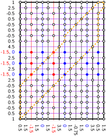
Figure 9: Left: The realisation of $\mathcal{U}$ for assignment $x_{1}=\textsf{True}$, $x_{2}=\textsf{True}$, $x_{3}=\textsf{False}$ and curve $\mathcal{V}$ for the formula $C=(x_{1}\lor x_{3})\land(\neg x_{1}\lor x_{2}\lor\neg x_{3})$. Note that $C=\textsf{True}$ with this assignment, and that both feasible alignments give (discrete) Fréchet distance of $1.5$. Right: The corresponding free space. White dots are accessible, spots without a dot are never accessible. Blue (red) dots are only accessible if the corresponding variable is set to True (False). Yellow dashed paths indicate potential paths through the free space; the goal is to determine if the variables can be set such that all potential paths are blocked.

Theorem 5.8.

The problem Upper Bound (Discrete) Fréchet is NP-hard in the indecisive model.

Proof 5.9.

First of all, notice that in our construction the synchronisation points at the start of the clauses gadgets must be matched to the synchronisation points at the start of the variable section and the $\mathrm{abs}$ gadgets in the optimal matching, as hinted at in the proofs of the previous lemmas. Furthermore, note that any number of $\mathrm{abs}^{2}$ at the start can be matched to the point at $1$, and any number of $\mathrm{abs}^{2}$ can be matched to the point at $1$ at the end. Putting these observations together with Lemmas 5.2, 5.4 and 5.6, it is easy to see the following. Choose some assignment $a$ and consider the corresponding realisation $\pi\Subset\mathcal{U}$. Suppose that $C[a]=\textsf{False}$; this means that there is at least one $i$ for which $C_{i}[a]=\textsf{False}$. Our construction allows us to consider the alignment where we match $\mathrm{CG}_{i}$ to $\mathrm{VS}$, and the rest of clauses to one of $\mathrm{abs}$; the remaining $\mathrm{abs}$ are matched to the $\mathrm{abs}^{2}$, and the remaining $\mathrm{abs}^{2}$ are matched to $1$. In this matching, the (discrete) Fréchet distance between the curves is $1$, which is optimal, and the formula is not satisfied. Now suppose that $C[a]=\textsf{True}$; this means that for all $i$, $C_{i}[a]=\textsf{True}$. So, no matter which $\mathrm{CG}_{i}$ we choose to align with $\mathrm{VS}$, we get the distance of $1.5$; therefore, the formula is satisfied, and the optimal distance is $1.5$.

Recall that the upper bound distance takes the maximum distance over all realisations. Therefore, if the upper bound distance is $1$, then all the realisations yield the distance $1$, and so all assignments $a$ yield $C[a]=\textsf{False}$, and the formula is not satisfiable. On the other hand, if the upper bound distance is $1.5$, then there is some realisation that yields this distance, and it corresponds to an assignment $a$ with $C[a]=\textsf{True}$, so the formula is satisfiable. Thus, our construction with the threshold $\delta=1$ solves CNF-SAT. Curve $\mathcal{U}$ has length $2+2\cdot(n-1)\cdot(1+2m)+1+2m=2n+4mn-2m+1$; curve $\mathcal{V}$ has length $4\cdot(n-1)+n\cdot(1+2m)=5n+2mn-4$. Clearly, the construction takes polynomial time. Therefore, the problem both for discrete and continuous Fréchet distance is NP-hard.

We can easily extend this result to the imprecise curves. We replace the indecisive points at $\{-1.5,0\}$ with intervals $[-1.5,0]$. The following observation is key. Any upper bound solution that can be found as a certificate in the construction with the indecisive points can also be found in the imprecise construction. Furthermore, note that no realisation can yield a distance above $1.5$ with an optimal matching. Thus, if the formula is satisfiable, the upper bound distance is still $1.5$, and this distance cannot be obtained otherwise. We conclude that the problem is NP-hard.

Theorem 5.10.

The problem Upper Bound (Discrete) Fréchet is NP-hard in the imprecise model.

6 Weak Fréchet Distance

In this section, we investigate the weak Fréchet distance for uncertain curves. In general, since weak matchings can revisit parts of the curve, the dynamic program for the regular Fréchet distance cannot easily be adapted, as it relies on the fact that only the realisation of the last few vertices is tracked. In particular, when computing the weak Fréchet distance for uncertain curves, one cannot simply forget the realisations of previously visited vertices, as the matching might revisit them. Surprisingly, we can show that for the continuous weak Fréchet distance between uncertain one-dimensional curves, we can still obtain a polynomial-time dynamic program, as shown in Section 6.1. One may expect that the discrete weak Fréchet distance for uncertain curves in 1D is also solvable in polynomial time; however, in Section 6.2 we show that this problem is NP-hard. We also show that computing the continuous weak Fréchet distance is NP-hard for uncertain curves in 2D.

6.1 Algorithm for Continuous Setting

We first introduce some definitions. Consider polygonal one-dimensional curves $\pi\colon[1,m]\to\mathbb{R}$ and $\sigma\colon[1,n]\to\mathbb{R}$ with vertices at the integer parameters. Let $\pi^{\raisebox{-2.0pt}{$\scriptscriptstyle-1$}}$ denote the reversal of a polygonal curve $\pi$. Denote by $\pi|_{[a,b]}$ the restriction of $\pi$ to the domain $[a,b]$. For integer values of $a$ and $b$, note that $\pi|_{[a,b]}\equiv\pi[a:b]$. Finally, define the image of a curve as the set of points in $\mathbb{R}$ that belong to the curve, $\mathrm{Im}(\pi)\equiv\{\pi(x)\mid x\in[1,m]\}$ for $\pi\colon[1,m]\to\mathbb{R}$. For any polygonal curve $\pi$, define the growing curve $\overrightarrow{\pi}$ of $\pi$ as the sequence of local minima and maxima of the sequence $\langle\pi(i)\mid\pi(i)\notin\mathrm{Im}(\pi|_{[1,i)})\rangle_{i=1}^{m}$. Thus, the vertices of a growing curve alternate between local minima and maxima, the subsequence of local maxima is strictly increasing, and the subsequence of local minima is strictly decreasing.

It has been shown that for precise one-dimensional curves, the weak Fréchet distance can be computed in linear time [15]. For uncertain curves, it is unclear how to use that linear-time algorithm; however, we can apply some of the underlying ideas. A relaxed matching between $\pi$ and $\sigma$ is defined by parametrisations $\alpha\colon[0,1]\to[1,m]$ and $\beta\colon[0,1]\to[1,n]$ with $\alpha(0)=1$, $\alpha(1)=x\in[m-1,m]$ and $\beta(0)=1$, $\beta(1)=y\in[n-1,n]$. Observe that the final points of parametrisations have to be on the last segments of the curves, but not necessarily at the endpoints of those segments. Moreover, define a relaxed matching $(\alpha,\beta)$ to be cell-monotone if for all $t\leq t^{\prime}$, we have $\min(\lfloor\alpha(t)\rfloor,m-1)\leq\alpha(t^{\prime})$ and $\min(\lfloor\beta(t)\rfloor,n-1)\leq\beta(t^{\prime})$. In other words, once we pass by a vertex to the next segment on a curve, we do not allow going back to the previous segment; backtracking within a segment is allowed. Let $\mathit{rm}(\pi,\sigma)$ be the minimum matching cost over all cell-monotone relaxed matchings:

$$\mathit{rm}(\pi,\sigma)=\inf_{\text{cell-monotone relaxed matching }\mu}\mathrm{cost}_{\mu}(\pi,\sigma)\,.$$

It has been shown for precise curves [15] that

$$d_{\mathrm{wF}}(\pi,\sigma)=\max\big{(}\mathit{rm}(\overrightarrow{\pi},\overrightarrow{\sigma}),\mathit{rm}(\overrightarrow{\pi^{\raisebox{-2.0pt}{$\scriptscriptstyle-1$}}},\overrightarrow{\sigma^{\raisebox{-2.0pt}{$\scriptscriptstyle-1$}}})\big{)}\,.$$

Let $\mathit{rm}(\pi,\sigma)[i,j]\equiv\mathit{rm}(\pi[1:i],\sigma[1:j])$. Then the value of $\mathit{rm}(\pi,\sigma)$ can be computed in quadratic time as $\mathit{rm}(\pi,\sigma)[m,n]$ using the following dynamic program:

$$\mathit{rm}(\pi,\sigma)[0,\cdot]=\mathit{rm}(\pi,\sigma)[\cdot,0] =\infty\,,$$

$$\mathit{rm}(\pi,\sigma)[1,1] =\lvert\pi(1)-\sigma(1)\rvert\,,\text{ and for $i>0$ or $j>0$,}$$

$$\mathit{rm}(\pi,\sigma)[i+1,j+1] =\min\left\{\begin{aligned} \max\big{(}\mathit{rm}(\pi,\sigma)[i,j+1],d\big{(}\pi(i),\mathrm{Im}(\sigma[j:j+1])\big{)}\big{)}\,,\\ \max\big{(}\mathit{rm}(\pi,\sigma)[i+1,j],d\big{(}\sigma(j),\mathrm{Im}(\pi[i:i+1])\big{)}\big{)}\,.\end{aligned}\right.$$

If $\pi$ is a growing curve, we have $\mathrm{Im}(\pi[i,i+1])=\mathrm{Im}(\pi[1:i+1])$, so the following dynamic program is equivalent if $\pi$ and $\sigma$ are growing curves:

$$r(\pi,\sigma)[0,\cdot]=r(\pi,\sigma)[\cdot,0] =\infty\,,$$

$$r(\pi,\sigma)[1,1] =\lvert\pi(1)-\sigma(1)\rvert\,,\text{ and for $i>0$ or $j>0$,}$$

$$r(\pi,\sigma)[i+1,j+1] =\min\begin{cases}\max\big{(}r(\pi,\sigma)[i,j+1],d\big{(}\pi(i),\mathrm{Im}(\sigma[1:j+1])\big{)}\big{)}\,,\\ \max\big{(}r(\pi,\sigma)[i+1,j],d\big{(}\sigma(j),\mathrm{Im}(\pi[1:i+1])\big{)}\big{)}\,.\end{cases}$$

Let $r(\pi,\sigma)\coloneqq r(\pi,\sigma)[m,n]$ when executing the dynamic program above for curves $\pi\colon[1,m]\to\mathbb{R}$ and $\sigma\colon[1,n]\to\mathbb{R}$. We have $\mathit{rm}(\overrightarrow{\pi},\overrightarrow{\sigma})=r(\overrightarrow{\pi},\overrightarrow{\sigma})$. Moreover, observe that the final result of computing $r$ is the same whether we apply it to the original or the growing curves. In other words, $r(\pi,\sigma)=r(\overrightarrow{\pi},\overrightarrow{\sigma})$, so

$$d_{\mathrm{wF}}(\pi,\sigma) =\max\big{(}\mathit{rm}(\overrightarrow{\pi},\overrightarrow{\sigma}),\mathit{rm}(\overrightarrow{\pi^{\raisebox{-2.0pt}{$\scriptscriptstyle-1$}}},\overrightarrow{\sigma^{\raisebox{-2.0pt}{$\scriptscriptstyle-1$}}})\big{)}$$

$$=\max\big{(}r(\overrightarrow{\pi},\overrightarrow{\sigma}),r(\overrightarrow{\pi^{\raisebox{-2.0pt}{$\scriptscriptstyle-1$}}},\overrightarrow{\sigma^{\raisebox{-2.0pt}{$\scriptscriptstyle-1$}}})\big{)}$$

$$=\max\big{(}r(\pi,\sigma),r(\pi^{\raisebox{-2.0pt}{$\scriptscriptstyle-1$}},\sigma^{\raisebox{-2.0pt}{$\scriptscriptstyle-1$}})\big{)}\,.$$

With regard to computing the minimum weak Fréchet distance over realisations of uncertain curves, this roughly means that we only need to keep track of the image of the prefix (and he suffix) of $\pi$ and $\sigma$. To formalise this, we split up the computation over the prefix and the suffix. Let $i_{\min},i_{\max}\in[m]$, $j_{\min},j_{\max}\in[n]$, $[x_{\min},x_{\max}]\subseteq\mathbb{R}$, and $[y_{\min},y_{\max}]\subseteq\mathbb{R}$. Abbreviate the pairs $I:=(i_{\min},i_{\max})$, $J:=(j_{\min},j_{\max})$ and the intervals $X:=[x_{\min},x_{\max}]$, $Y:=[y_{\min},y_{\max}]$, and call a realisation $\pi$ of an uncertain curve $I$-respecting if $\pi(i_{\min})$ is a global minimum of $\pi$ and $\pi(i_{\max})$ is a global maximum of $\pi$. Moreover, say that $\pi$ is $(I,X)$-respecting if additionally $\pi(i_{\min})=x_{\min}$ and $\pi(i_{\max})=x_{\max}$. Let $\pi^{\prime}\Subset\mathcal{U}_{I}$ and $\pi^{\prime\prime}\Subset\mathcal{U}_{I}^{X}$ denote some $I$- and $(I,X)$-respecting realisations of an uncertain curve $\mathcal{U}$, respectively. Consider the minimum weak Fréchet distance between $(I,X)$- and $(J,Y)$-respecting realisations $\pi\Subset\mathcal{U}_{I}^{X}$ and $\sigma\Subset\mathcal{V}_{J}^{Y}$:

$$d_{\mathrm{wF}}^{\,\min}(\mathcal{U}_{I}^{X},\mathcal{V}_{J}^{Y})\equiv\min_{\pi\Subset\mathcal{U}_{I}^{X},\sigma\Subset\mathcal{V}_{J}^{Y}}d_{\mathrm{wF}}(\pi,\sigma)=\min_{\pi\Subset\mathcal{U}_{I}^{X},\sigma\Subset\mathcal{V}_{J}^{Y}}\max\big{(}r(\pi,\sigma),r(\pi^{\raisebox{-2.0pt}{$\scriptscriptstyle-1$}},\sigma^{\raisebox{-2.0pt}{$\scriptscriptstyle-1$}})\big{)}\,.$$

Lemma 6.1.

Among $(I,X)$- and $(J,Y)$-respecting realisations, the prefix and the suffix are independent:

$$d_{\mathrm{wF}}^{\,\min}(\mathcal{U}_{I}^{X},\mathcal{V}_{J}^{Y})=\max\begin{cases}\min_{\pi\Subset\mathcal{U}_{I}^{X},\sigma\Subset\mathcal{V}_{J}^{Y}}r(\pi,\sigma)\,,\\ \min_{\pi^{\prime}\Subset\mathcal{U}_{I}^{X},\sigma^{\prime}\Subset\mathcal{V}_{J}^{Y}}r(\pi^{\prime\raisebox{-2.0pt}{$\scriptscriptstyle-1$}},\sigma^{\prime\raisebox{-2.0pt}{$\scriptscriptstyle-1$}})\,.\end{cases}$$

Proof 6.2.

If we take $\pi=\pi^{\prime}$ and $\sigma=\sigma^{\prime}$, the right-hand side becomes a lower bound on $d_{\mathrm{wF}}^{\,\min}(\mathcal{U}_{I}^{X},\mathcal{V}_{J}^{Y})$. To show that it is also an upper bound, consider $(I,X)$-respecting realisations $\pi$ and $\pi^{\prime}$, and define $\pi_{c}$ as the prefix of $\pi$ up to $i_{\min}$ concatenated with the suffix of $\pi^{\prime}$ starting from $i_{\min}$. Then $\pi_{c}$ is an $(I,X)$-respecting realisation of $\mathcal{U}$. Moreover, the growing curves $\overrightarrow{\pi}$ and $\overrightarrow{\pi_{c}}$ are the same (this is obvious if $i_{\min}>i_{\max}$, and follows from the fact that the value of the $i_{\max}$-th vertex is $x_{\max}$ otherwise). Symmetrically, $\overrightarrow{\pi^{\prime\raisebox{-2.0pt}{$\scriptscriptstyle-1$}}}=\overrightarrow{\pi_{c}^{\raisebox{-2.0pt}{$\scriptscriptstyle-1$}}}$. We can similarly define a $(J,Y)$-respecting realisation $\sigma_{c}$ of $\mathcal{V}$ based on some $\sigma$ and $\sigma^{\prime}$. Since $\overrightarrow{\pi}=\overrightarrow{\pi_{c}}$ and $\overrightarrow{\sigma}=\overrightarrow{\sigma_{c}}$, we have $r(\pi,\sigma)=r(\pi_{c},\sigma_{c})$, and symmetrically, $r(\pi^{\prime\raisebox{-2.0pt}{$\scriptscriptstyle-1$}},\sigma^{\prime\raisebox{-2.0pt}{$\scriptscriptstyle-1$}})=r(\pi_{c}^{\raisebox{-2.0pt}{$\scriptscriptstyle-1$}},\sigma_{c}^{\raisebox{-2.0pt}{$\scriptscriptstyle-1$}})$. We can therefore use $\pi_{c}\Subset\mathcal{U}_{I}^{X}$ and $\sigma_{c}\Subset\mathcal{V}_{J}^{Y}$ in the definition of $d_{\mathrm{wF}}(\mathcal{U}_{I}^{X},\mathcal{V}_{J}^{Y})$ to obtain the desired upper bound.

The remainder of this section is guided by the following observations based on Lemma 6.1.

1. If we can compute $\min_{\pi\Subset\mathcal{U}_{I}^{X},\sigma\Subset\mathcal{V}_{J}^{Y}}r(\pi,\sigma)$, we can compute $d_{\mathrm{wF}}^{\,\min}(\mathcal{U}_{I}^{X},\mathcal{V}_{J}^{Y})$.

2. To compute $d_{\mathrm{wF}}^{\,\min}(\mathcal{U}_{I},\mathcal{V}_{J})$, we must find an optimal pair of images $X$ and $Y$ for $\pi$ and $\sigma$.

3. We can find $d_{\mathrm{wF}}^{\,\min}(\mathcal{U},\mathcal{V})$ by computing $d_{\mathrm{wF}}^{\,\min}(\mathcal{U}_{I},\mathcal{V}_{J})$ for all $O(m^{2}n^{2})$ values for $(I,J)$.

Instead of computing $\min_{\pi\Subset\mathcal{U}_{I}^{X},\sigma\Subset\mathcal{V}_{J}^{Y}}r(\pi,\sigma)$ for a specific value of $(X,Y)$, we compute the function $(X,Y)\mapsto\min_{\pi\Subset\mathcal{U}_{I}^{X},\sigma\Subset\mathcal{V}_{J}^{Y}}r(\pi,\sigma)$ using a dynamic program that effectively simulates the dynamic program $r(\pi,\sigma)$ for all $I$- and $J$-respecting realisations simultaneously. So let

$$R_{I,J}[i,j](x,y,X,Y):= \inf_{\begin{subarray}{c}\pi\Subset\mathcal{U}_{I},\mathrm{Im}(\pi[1:i])=X,\pi(i)=x\\ \sigma\Subset\mathcal{V}_{J},\mathrm{Im}(\sigma[1:j])=Y,\sigma(j)=y\end{subarray}}r(\pi,\sigma)[i,j],\quad\text{then}$$

$$R_{I,J}[m,n](x,y,X,Y)= \inf_{\begin{subarray}{c}\pi\Subset\mathcal{U}_{I}^{X},\pi(m)=x\\ \sigma\Subset\mathcal{V}_{J}^{Y},\sigma(n)=y\end{subarray}}r(\pi,\sigma).$$

We derive

$$R_{I,J}[0,\cdot](x,y,X,Y)=R_{I,J}[\cdot,0](x,y,X,Y)=\infty,$$

$$R_{I,J}[1,1](x,y,X,Y)=\inf_{\begin{subarray}{c}\pi\Subset\mathcal{U}_{I},\{x\}=X,\pi(1)=x\\ \sigma\Subset\mathcal{V}_{J},\{y\}=Y,\sigma(1)=y\end{subarray}}\lvert\pi(1)-\sigma(1)\rvert,\text{ and for $(i,j)\neq(1,1)$}$$

$$R_{I,J}[i,j](x,y,X,Y)$$

$$\quad=\inf_{\begin{subarray}{c}\pi\Subset\mathcal{U}_{I},\mathrm{Im}(\pi[1:i])=X,\pi(i)=x\\ \sigma\Subset\mathcal{V}_{J},\mathrm{Im}(\sigma[1:j])=Y,\sigma(j)=y\end{subarray}}\min\begin{cases}\max\{r(\pi,\sigma)[i-1,j],d(\pi(i-1),Y)\},\\ \max\{r(\pi,\sigma)[i,j-1],d(\sigma(j-1),X)\}\end{cases}$$

$$\quad=\min\begin{cases}\inf_{\begin{subarray}{c}\pi\Subset\mathcal{U}_{I},\mathrm{Im}(\pi[1:i])=X,\pi(i)=x\\ \sigma\Subset\mathcal{V}_{J},\mathrm{Im}(\sigma[1:j])=Y,\sigma(j)=y\\ \pi(i-1)=x^{\prime}\end{subarray}}\max\{r(\pi,\sigma)[i-1,j],d(x^{\prime},Y)\},\\ \inf_{\begin{subarray}{c}\pi\Subset\mathcal{U}_{I},\mathrm{Im}(\pi[1:i])=X,\pi(i)=x\\ \sigma\Subset\mathcal{V}_{J},\mathrm{Im}(\sigma[1:j])=Y,\sigma(j)=y\\ \sigma(j-1)=y^{\prime}\end{subarray}}\max\{r(\pi,\sigma)[i,j-1],d(y^{\prime},X)\}\end{cases}$$

$$\quad=\min\begin{cases}\inf_{\begin{subarray}{c}\pi\Subset\mathcal{U}_{I},\mathrm{Im}(\pi[1:i])=X,\pi(i)=x\\ \mathrm{Im}(\pi[1:i-1])=X^{\prime},\pi(i-1)=x^{\prime}\end{subarray}}\max\{R_{I,J}[i-1,j](x^{\prime},y,X^{\prime},Y),d(x^{\prime},Y)\},\\ \inf_{\begin{subarray}{c}\sigma\Subset\mathcal{V}_{J},\mathrm{Im}(\sigma[1:j])=Y,\sigma(j)=y\\ \mathrm{Im}(\sigma[1:j-1])=Y^{\prime},\sigma(j-1)=y^{\prime}\end{subarray}}\max\{R_{I,J}[i,j-1](x,y^{\prime},X,Y^{\prime}),d(y^{\prime},X)\},\end{cases}$$

where, crucially, the conditions on $x^{\prime}$, $y^{\prime}$, $X^{\prime}$, and $Y^{\prime}$ can be checked purely in terms of $\mathcal{U}_{I}$ and $\mathcal{V}_{J}$, so the recurrence does not depend on any particular $\pi$ or $\sigma$. This yields a dynamic program that constructs the function $R_{I,J}[i,j]$ based on the functions $R_{I,J}[i-1,j]$ and $R_{I,J}[i,j-1]$.

The recurrence has the parameters $I$, $J$, $i$, $j$, $x$, $y$, $X$, and $Y$. The first four are easy to handle, since $i\in[m]$, $j\in[n]$, $I\in[m]^{2}$, and $J\in[n]^{2}$. The other parameters are continuous. $X$ can be represented by $x_{\min}$ and $x_{\max}$, $Y$ by $y_{\min}$ and $y_{\max}$. To prove that we can solve the recurrence in polynomial time, it is sufficient to prove that we can restrict the computation to a polynomial number of different $x_{\min}$, $x_{\max}$, $y_{\min}$, $y_{\max}$, $x$ and $y$.

We assume that each of the $u_{i}$ and $v_{j}$ is given as a set of intervals. This includes the cases of uncertain curves with imprecise vertices (where each of these is just one interval) and with indecisive vertices (where each interval is just a point; but in this case we get by definition only a polynomial number of different values for the parameters).

Consider the realisations $\pi=\langle p_{1},\dots,p_{m}\rangle$ and $\sigma=\langle q_{1},\dots,q_{n}\rangle$ of the curves that attain the lower bound weak Fréchet distance $d_{\mathrm{wF}}^{\,\min}(\mathcal{U},\mathcal{V})=:\delta$. In these realisations, we need to have a sequence of vertices $r_{1}\leq r_{2}\leq\dots\leq r_{\ell}$ with the $r_{k}$ alternately from the set of $p_{i}$ and the set of $q_{j}$ such that $r_{1}$ is at a right interval endpoint, $r_{\ell}$ is at a left interval endpoint, and $r_{k+1}-r_{k}=\delta$. Since $1\leq\ell\leq m+n$, this implies that there are only $O(N^{2}\cdot(m+n))$ candidates for $\delta$, where $N$ is the total number of interval endpoints. We can compute these candidates in time $O(N^{2}\cdot(m+n))$.

Now assume that we have chosen $\pi$ and $\sigma$ such that none of the $p_{i}$ or $q_{j}$ can be increased (i.e. moved to the right) without increasing the weak Fréchet distance. Then for every $p_{i}$ (and likewise $q_{j}$) there is a sequence $r_{1}\leq r_{2}\leq\dots\leq r_{\ell}=p_{i}$, where $r_{1}$ is the endpoint of an interval and $r_{k+1}-r_{k}=\delta$. There are $O(N)$ possibilities for $r_{1}$, $O(m+n)$ possibilities for $\ell$, and $O(N^{2}\cdot(m+n))$ possibilities for $\delta$, thus the total number of positions to consider for $p_{i}$ is polynomial.

Theorem 6.3.

The continuous weak Fréchet distance between uncertain one-dimensional curves can be computed in polynomial time.

6.2 Hardness of Discrete Setting

In this section, we prove that minimising the discrete weak Fréchet distance is NP-hard, already in one-dimensional space. We show this both in the model where uncertainty regions are discrete point sets and in the model where they are intervals.

In the constructions in this section, the lower bound Fréchet distance is never smaller than $1$. The goal is to determine whether it is equal to $1$ or greater than $1$.

6.2.1 Indecisive Points

We reduce from 3SAT. Consider an instance with $n$ variables and $m$ clauses. We assign each variable a unique height (coordinate in the one-dimensional space): variable $x_{i}$ gets assigned height $10i+5$. We use slightly higher heights ($10i+6$ and $10i+7$) to interact with a positive state of the variable, and slightly lower heights to interact with a negative state.

We construct two uncertain curves, one which represents the variables and one which represents the clauses. The first curve, $\mathcal{U}$, consists of $n+2$ vertices. The first and last vertex are certain points, both at height $0$. The remaining vertices are uncertain points, with two possible heights each:

$$\mathcal{U}=\langle 0,\{14,16\},\{24,26\},\dots,\{10n+4,10n+6\},0\rangle\,.$$

The second curve, $\mathcal{V}$, consists of $nm+n+m+2$ vertices. For clause $c_{j}=\ell_{a}\lor\ell_{b}\lor\ell_{c}$, let $C_{j}$ be the set $\{10a+3/7,10b+3/7,10c+3/7\}$, where for each literal we choose $+3$ if $\ell_{i}=x_{i}$ or $+7$ if $\ell_{i}=\neg x_{i}$. Let $S$ be the set $S=\{15,25,\dots,10n+5\}$ of ‘neutral’ variable heights. Then $\mathcal{V}$ is the curve that starts and ends at $0$, has a vertex for each $C_{j}$, and has sufficiently many copies of $S$ between them:

$$\mathcal{V}=\langle 0,S,\dots,S,C_{1},S,\dots,S,C_{2},S,\dots,S,\dots\dots,C_{m},0\rangle\,.$$

Consider the free-space diagram, with a ‘spot’ $(i,j)$ corresponding to each pair of vertices $u_{i}$ and $v_{j}$. The discrete weak Fréchet distance is equal to $1$ if and only if there is an assignment to each uncertain vertex such that the there is a path from the bottom left to the top right of the diagram that uses only accessible spots, where a spot is accessible if the assigned heights of the corresponding row and column are within $1$. Figure 10 shows an example.

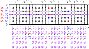
Figure 10: An example with five variables and three clauses. White dots are always accessible, no matter the state of the variables (however, note that only one white dot per column can be used). Red / blue dots are accessible only if the corresponding variable is set to False / True. Spots without a dot are never accessible.

We can only cross a column corresponding to clause $c_{j}$ if at least one of the corresponding literals is set to true. The remaining columns can always be crossed at any row. Note that the repetition is necessary: although all spots are in principle reachable, only one spot in each column can be reachable at the same time. If we have at least $n$ columns between each pair of clauses, this will always be possible.

Theorem 6.4.

Given two uncertain curves $\mathcal{U}$ and $\mathcal{V}$, each given by a sequence of values and sets of values in $\mathbb{R}$, the problem of choosing a realisation of $\mathcal{U}$ and $\mathcal{V}$ such that the weak discrete Fréchet distance between $\mathcal{U}$ and $\mathcal{V}$ is minimised is NP-hard.

6.2.2 Imprecise Points

The construction above relies heavily on the ability to select arbitrary sets of values as uncertainty regions. We now show that this is not required. We strengthen the proof in two ways: we restrict the uncertainty regions to be connected intervals, and we use uncertainty in only one of the curves.

The main idea of the adaptation is to encode clauses not by a single uncertain vertex, but by sets of globally distinct paths through the free-space diagram. To facilitate this, we need a global frame to guide the possible solution paths, and we need more copies of the variable vertices (though only one copy will be uncertain) to facilitate the paths.

Let $T=10(n+2)$. We build a frame for the construction using four unique heights: $0$, $10$, $T-10$ and $T$. Let $S=\langle 0,10,?,T-10,?,10,?,T-10,T\rangle$ be a partial sequence – the question marks indicate gaps where we insert other vertices later. Globally, the curves have the structure $\mathcal{U}=S$ and $\mathcal{V}=S\sqcup S^{-1}\sqcup S\sqcup S^{-1}\sqcup\dots\sqcup S$: one copy or reversed copy of $S$ for each clause (if the number of clauses is even, simply add a trivial clause). In the free-space diagram, this creates a frame that every path needs to adhere to. The frame consists of one block per clause, and inside each block, there are three potential paths from the bottom left to top right corner (or from the top left to bottom right corner for reversed blocks). See Figure 11.

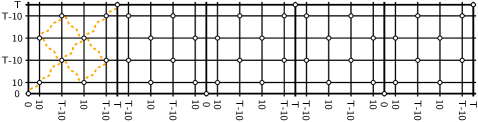
Figure 11: The global frame. White dots are accessible, spots without a dot are never accessible. Within each block, there are three potential paths between its two accessible corners.

Next, we fill in the gaps. Let $\mathcal{U}=\mathcal{U}_{1}\sqcup\mathcal{U}_{2}^{-1}\sqcup\mathcal{U}_{1}$, where

$$\mathcal{U}_{1} =\langle 0,10,14,16,24,26,\dots,10n+4,10n+6,T-10,T\rangle\,,$$

$$\mathcal{U}_{2} =\langle 0,10,[14,16],[24,26],\dots,[10n+4,10n+6],T-10,T\rangle\,.$$

Let $\mathcal{V}=\bigsqcup_{1\leq j\leq m}C_{j}^{(-1)^{j-1}}$ be concatenation of clause sequences, where each even clause sequence is reversed. For a clause $c_{j}=\ell_{a}\lor\ell_{b}\lor\ell_{c}$, the sequence $C_{j}$ is of the form

$$C_{j}=\langle 0,10\rangle\sqcup L_{a}\sqcup\langle T-10\rangle\sqcup L_{b}^{-1}\sqcup\langle 10\rangle\sqcup L_{c}\sqcup\langle T-10,T\rangle\,,$$

where the literal sequence $L_{i}$ corresponding to $\ell_{i}=x_{i}$ (positive literals) or $\ell_{i}=\neg x_{i}$ (negative literals) is respectively

$$L_{i} =\langle 15,25,\dots,10(i-1)+5,10i+5,10i+7,10(i+1)+5,\dots,10n+5\rangle\,,\quad\text{or}$$

$$L_{i} =\langle 15,25,\dots,10(i-1)+5,10i+3,10i+5,10(i+1)+5,\dots,10n+5\rangle\,.$$

See Figure 12 for an example of the resulting free-space diagram.

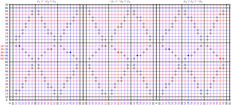
Figure 12: An example with five variables and three clauses. White dots are always accessible, no matter the state of the variables. Red / blue dots are accessible only if the corresponding variable is set to False / True. Spots without a dot are never accessible.

The construction relies on the following. $L_{i}$ can always be matched to $\mathcal{U}_{1}$. $L_{i}$ can be matched to $\mathcal{U}_{2}$ if and only if $\ell_{i}=x_{i}$ and $x_{i}$ is set to True, or $\ell_{i}=\neg x_{i}$ and $x_{i}$ is set to False.

Theorem 6.5.

Given an uncertain curve $\mathcal{U}$, given by a sequence of values and intervals in $\mathbb{R}$, and a certain curve $\mathcal{V}$, given by a sequence of values in $\mathbb{R}$, the problem of choosing a realisation of $\mathcal{U}$ such that the weak discrete Fréchet distance between $\mathcal{U}$ and $\mathcal{V}$ is minimised is NP-hard.

6.2.3 Continuous Weak Fréchet Distance in $\mathbb{R}^{2}$

Finally, we mention that the results in this section carry over to continuous weak Fréchet distance in one dimension higher. We simply construct the same curves as described above on the $x$-axis, and intersperse each curve with the point at $(0,\infty)$.

Corollary 6.6.

Given an uncertain curve $\mathcal{U}$, given by a sequence of points and regions in $\mathbb{R}^{2}$, and a certain curve $\mathcal{V}$, given by a sequence of points in $\mathbb{R}^{2}$, the problem of choosing a realisation of $\mathcal{U}$ such that the weak Fréchet distance between $\mathcal{U}$ and $\mathcal{V}$ is minimised is NP-hard.

References

- [1] Manuel Abellanas, Ferran Hurtado, Christian Icking, Rolf Klein, Elmar Langetepe, Lihong Ma, Belén Palop, and Vera Sacristán. Smallest color-spanning objects. In Algorithms – ESA 2001, volume 2161 of Lecture Notes in Computer Science, pages 278–289, Berlin, Germany, 2001. Springer Berlin Heidelberg. doi:10.1007/3-540-44676-1\_23.
- [2] Pankaj K. Agarwal, Rinat Ben Avraham, Haim Kaplan, and Micha Sharir. Computing the discrete Fréchet distance in subquadratic time. SIAM Journal on Computing, 43(2):429–449, 2014. doi:10.1137/130920526.
- [3] Mahmuda Ahmed and Carola Wenk. Constructing street networks from GPS trajectories. In Proceedings of 20th Annual European Symposium on Algorithms, volume 7501 of Lecture Notes in Computer Science, pages 60–71, Berlin, Germany, 2012. Springer Berlin Heidelberg. doi:10.1007/978-3-642-33090-2\_7.
- [4] Hee-Kap Ahn, Christian Knauer, Marc Scherfenberg, Lena Schlipf, and Antoine Vigneron. Computing the discrete Fréchet distance with imprecise input. International Journal of Computational Geometry & Applications, 22(01):27–44, 2012. doi:10.1142/S0218195912600023.
- [5] Helmut Alt and Michael Godau. Computing the Fréchet distance between two polygonal curves. International Journal of Computational Geometry and Applications, 5(1):75–91, 1995. doi:10.1142/S0218195995000064.
- [6] Sotiris Brakatsoulas, Dieter Pfoser, Randall Salas, and Carola Wenk. On map-matching vehicle tracking data. In Proceedings of the 31st International Conference on Very Large Data Bases, pages 853–864, New York, NY, USA, 2005. Association for Computing Machinery. doi:10.5555/1083592.1083691.
- [7] Karl Bringmann. Why walking the dog takes time: Fréchet distance has no strongly subquadratic algorithms unless SETH fails. In 2014 IEEE 55th Annual Symposium on Foundations of Computer Science, pages 661–670, Piscataway, NJ, USA, August 2014. IEEE. arXiv:1404.1448v2, doi:10.1109/FOCS.2014.76.
- [8] Karl Bringmann and Wolfgang Mulzer. Approximability of the discrete Fréchet distance. Journal of Computational Geometry, 7(2):46–76, 2016. doi:10.20382/jocg.v7i2a4.
- [9] Kevin Buchin, Maike Buchin, David Duran, Brittany Terese Fasy, Roel Jacobs, Vera Sacristán, Rodrigo I. Silveira, Frank Staals, and Carola Wenk. Clustering trajectories for map construction. In Proceedings of the 25th ACM SIGSPATIAL International Conference on Advances in Geographic Information Systems, pages 14:1–14:10, New York, NY, USA, 2017. Association for Computing Machinery. doi:10.1145/3139958.3139964.
- [10] Kevin Buchin, Maike Buchin, Christian Knauer, Günter Rote, and Carola Wenk. How difficult is it to walk the dog?, 2007. Presented at EuroCG 2007, Graz, Austria. URL: https://page.mi.fu-berlin.de/rote/Papers/pdf/How+difficult+is+it+to+walk+the+dog.pdf.
- [11] Kevin Buchin, Maike Buchin, Wouter Meulemans, and Wolfgang Mulzer. Four Soviets walk the dog: Improved bounds for computing the Fréchet distance. Discrete & Computational Geometry, 58(1):180–216, 2017. doi:10.1007/s00454-017-9878-7.
- [12] Kevin Buchin, Anne Driemel, Natasja van de L’Isle, and André Nusser. Klcluster: Center-based clustering of trajectories. In Proceedings of the 27th ACM SIGSPATIAL International Conference on Advances in Geographic Information Systems, SIGSPATIAL ’19, pages 496–499, New York, NY, USA, 2019. Association for Computing Machinery. doi:10.1145/3347146.3359111.
- [13] Kevin Buchin, Chenglin Fan, Maarten Löffler, Aleksandr Popov, Benjamin Raichel, and Marcel Roeloffzen. Fréchet distance for uncertain curves. In 47th International Colloquium on Automata, Languages, and Programming (ICALP 2020), volume 168 of Leibniz International Proceedings in Informatics (LIPIcs), pages 20:1–20:20, Dagstuhl, Germany, 2020. Schloss Dagstuhl–Leibniz-Zentrum für Informatik. arXiv:2004.11862, doi:10.4230/LIPIcs.ICALP.2020.20.
- [14] Kevin Buchin, Maarten Löffler, Pat Morin, and Wolfgang Mulzer. Preprocessing imprecise points for Delaunay triangulation: Simplified and extended. Algorithmica, 61(3):674–693, November 2011. doi:10.1007/s00453-010-9430-0.
- [15] Kevin Buchin, Tim Ophelders, and Bettina Speckmann. SETH says: Weak Fréchet distance is faster, but only if it is continuous and in one dimension. In Proceedings of the Thirtieth Annual ACM–SIAM Symposium on Discrete Algorithms (SODA ’19), pages 2887–2901. Society for Industrial and Applied Mathematics, January 2019. doi:10.5555/3310435.3310614.
- [16] Maike Buchin and Stef Sijben. Discrete Fréchet distance for uncertain points, 2016. Presented at EuroCG 2016, Lugano, Switzerland. URL: http://www.eurocg2016.usi.ch/sites/default/files/paper_72.pdf.
- [17] Anne Driemel, Sariel Har-Peled, and Carola Wenk. Approximating the Fréchet distance for realistic curves in near linear time. Discrete & Computational Geometry, 48(1):94–127, July 2012. doi:s00454-012-9402-z.
- [18] Chenglin Fan, Jun Luo, and Binhai Zhu. Tight approximation bounds for connectivity with a color-spanning set. In Algorithms and Computation (ISAAC 2013), volume 8283 of Lecture Notes in Computer Science, pages 590–600, Berlin, Germany, 2013. Springer Berlin Heidelberg. doi:10.1007/978-3-642-45030-3\_55.
- [19] Chenglin Fan and Binhai Zhu. Complexity and algorithms for the discrete Fréchet distance upper bound with imprecise input, February 2018. arXiv:1509.02576v2.
- [20] Joachim Gudmundsson and Thomas Wolle. Football analysis using spatio-temporal tools. Computers, Environment and Urban Systems, 47:16–27, 2014. doi:10.1016/j.compenvurbsys.2013.09.004.
- [21] Sariel Har-Peled and Benjamin Raichel. The Fréchet distance revisited and extended. ACM Transactions on Algorithms (TALG), 10(1):3:1–3:22, January 2014. doi:10.1145/2532646.
- [22] Minghui Jiang, Ying Xu, and Binhai Zhu. Protein structure: Structure alignment with discrete Fréchet distance. Journal of Bioinformatics and Computational Biology, 6(1):51–64, 2008. doi:10.1142/s0219720008003278.
- [23] Christian Knauer, Maarten Löffler, Marc Scherfenberg, and Thomas Wolle. The directed Hausdorff distance between imprecise point sets. Theoretical Computer Science, 412(32):4173–4186, 2011. doi:10.1016/j.tcs.2011.01.039.
- [24] Maarten Löffler. Data Imprecision in Computational Geometry. PhD thesis, Universiteit Utrecht, October 2009. URL: https://dspace.library.uu.nl/bitstream/handle/1874/36022/loffler.pdf [cited 2019-06-15].
- [25] Maarten Löffler and Wolfgang Mulzer. Unions of onions: Preprocessing imprecise points for fast onion decomposition. Journal of Computational Geometry (JoCG), 5(1):1–13, 2014. doi:10.20382/jocg.v5i1a1.
- [26] Maarten Löffler and Jack Snoeyink. Delaunay triangulations of imprecise points in linear time after preprocessing. Computational Geometry: Theory and Applications, 43(3):234–242, 2010. doi:10.1016/j.comgeo.2008.12.007.
- [27] Maarten Löffler and Marc van Kreveld. Largest and smallest tours and convex hulls for imprecise points. In Algorithm Theory – SWAT 2006, volume 4059 of Lecture Notes in Computer Science, pages 375–387, Berlin, Germany, 2006. Springer Berlin Heidelberg. doi:10.1007/11785293\_35.
- [28] Marc van Kreveld, Maarten Löffler, and Joseph S. B. Mitchell. Preprocessing imprecise points and splitting triangulations. SIAM Journal on Computing, 39(7):2990–3000, May 2010. doi:10.1137/090753620.
- [29] Jianbin Zheng, Xiaolei Gao, Enqi Zhan, and Zhangcan Huang. Algorithm of on-line handwriting signature verification based on discrete Fréchet distance. In International Symposium on Intelligence Computation and Applications, volume 5370 of Lecture Notes in Computer Science, pages 461–469, Berlin, Germany, 2008. Springer Berlin Heidelberg. doi:10.1007/978-3-540-92137-0\_5.