Pulse-level noisy quantum circuits with QuTiP
Abstract
The study of the impact of noise on quantum circuits is especially relevant to guide the progress of Noisy Intermediate-Scale Quantum (NISQ) computing. In this paper, we address the pulse-level simulation of noisy quantum circuits with the Quantum Toolbox in Python (QuTiP). We introduce new tools in qutip-qip, QuTiP’s quantum information processing package. These tools simulate quantum circuits at the pulse level, leveraging QuTiP’s quantum dynamics solvers and control optimization features. We show how quantum circuits can be compiled on simulated processors, with control pulses acting on a target Hamiltonian that describes the unitary evolution of the physical qubits. Various types of noise can be introduced based on the physical model, e.g., by simulating the Lindblad density-matrix dynamics or Monte Carlo quantum trajectories. In particular, the user can define environment-induced decoherence at the processor level and include noise simulation at the level of control pulses. We illustrate how the Deutsch-Jozsa algorithm is compiled and executed on a superconducting-qubit-based processor, on a spin-chain-based processor and using control optimization algorithms. We also show how to easily reproduce experimental results on cross-talk noise in an ion-based processor, and how a Ramsey experiment can be modeled with Lindblad dynamics. Finally, we illustrate how to integrate these features with other software frameworks.
1 Introduction
Quantum computation and quantum algorithms are deemed to be able to complete tasks that would be harder or impossible to achieve with classical resources. However, noise on quantum hardware significantly influences its performance, limiting large-scale applications. Currently, we are in the so-called noisy intermediate-scale quantum (NISQ) computing era [1]. Before we reach the regime of quantum error correction (QEC) [2], quantum algorithms will suffer from quantum and classical noise, e.g., decoherence and noise in classical control signals. Both types of noise lead to errors in the computation and therefore determine the performance of a quantum algorithm. Hence, a realistic simulation of a quantum algorithm needs to incorporate these different types of noise, which can depend strongly on the type of qubit technology [3].
A modern quantum algorithm typically includes both classical and quantum parts [4]. The former can include classical variational subroutines, while the latter is usually represented by a quantum circuit, consisting of a number of gates applied on a quantum state. Many software projects provide the simulation of such circuits including PyQuil [5, 6], Qiskit [7], Cirq [8], ProjectQ [9], and PennyLane [10], among others [11, 12]. However, within these approaches, noise is usually modelled as an additional layer on top of ideal quantum gates, e.g., probabilistically inserting random Pauli gates or a list of Kraus operators to describe a noisy quantum channel.
To improve the performance of a quantum circuit on noisy hardware, it is useful to also perform optimization at the level of control pulses based on the quantum dynamics of the underlying hardware. For this purpose, open-source software packages have been developed to map quantum circuits to control pulses on hardware, allowing for fine-tuning and calibration of the control pulses, such as qiskit.pulse [13], qctrl-open-controls [14] and Pulser [15]. Recently, Qiskit also launched the project qiskit-dynamics to support solving time-dependent quantum systems, connected with qiskit.pulse. The project is still in the early stages of development.
In the realm of simulation, one of the earliest, and most widely used Python packages to simulate quantum dynamics is the Quantum Toolbox in Python, QuTiP [16, 17]. QuTiP provides useful tools for handling quantum operators and simplifies the simulation of a quantum system under a noisy environment by providing a number of solvers, such as the Lindblad master equation solver. An ecosystem of software tools for quantum technology is growing around it [18, 19, 20, 21, 22, 23, 15, 24, 13, 25]. Hence, it is a natural base to start connecting the simulation of quantum circuits and the time evolution of the quantum system representing the circuit registers. At the cost of more computing resources, simulation at the level of time evolution allows noise based on the physical model to be included in the realistic study of quantum circuits.
Summary of results
In this paper, we illustrate how the new tools in qutip-qip111https://github.com/qutip/qutip-qip can be used to bridge the gap between the gate-level circuit simulation and the simulation of quantum dynamics following the master equation for various hardware models. While a quantum circuit representation and a few specific Hamiltonian models have been available in QuTiP for some time, in this paper, we bridge them with QuTiP solvers and build a pulse-level simulation framework, allowing the simulation of noisy circuits.
Provided a Hamiltonian model and a map between the quantum gate and control pulses, we show how these new tools in qutip-qip can be used to compile the circuit into the native gates of a given hardware, how to generate the physical model described by control pulses and how to use QuTiP’s dynamical solvers to obtain the full-state time evolution, as shown in Figure 1.
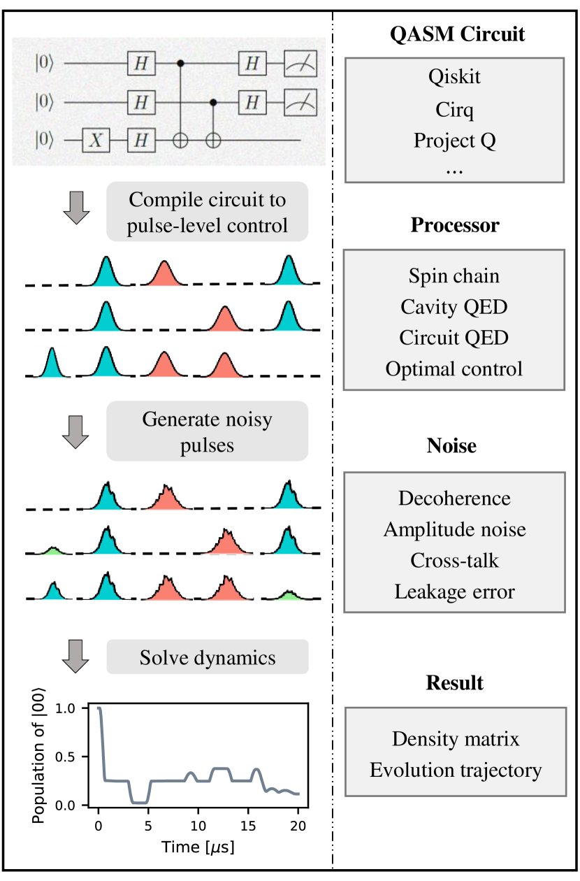
A number of example hardware models are available in the software package – a spin qubit processor, a cavity-QED device, a superconducting qubit model – while in general the users are provided with the freedom to define their own devices of choice.
In addition to a predefined map between gates and pulses for each model, optimal control algorithms in QuTiP can also be used to generate control pulses. Moreover, we demonstrate how various types of noise, including decoherence induced by the quantum environment and classical control noise, can be introduced at different layers of the simulation. Thanks to a modular code design, one can quickly extend the toolkit with customized hardware and noise models.
Article structure
The article is organized as follows: In Section 2, information about the software installation and specifics is given. In Section 3, we briefly present the background concepts of quantum circuits at the gate level, the continuous-time pulse-level description for circuits, open quantum systems theory and the tools present in qutip and qutip-qip to represent and simulate open quantum systems. Section 4 contains the main novel results and new software features: therein, we illustrate in detail the novel architecture of the pulse-level quantum-circuit simulation framework in qutip-qip and the available modelling of quantum devices and noise. In Section 5, we show how these features can be integrated with other software through importing external quantum circuits using the QASM format. We conclude in Section 6.
The Appendices include self-contained code examples: Appendix A contains the full code for the Deutsch-Jozsa algorithm simulation; Appendix B presents the simulation of a 10-qubit quantum Fourier transform (QFT) algorithm using the spin chain model; Appendix C shows how to customize the physical model of a processor with noise. More examples can also be found in QuTiP tutorials222http://qutip.org/tutorials.html under the section Quantum Information Processing.
2 Software information
The tools described here are part of the QuTiP project [16, 17].
The qutip-qip package builds upon what was once a module of QuTiP, qutip.qip.
Usage and installation has not significantly changed for the end user, who can easily install the package from the Python package index (PyPI) distribution with
The qutip-qip package has the core qutip package as its main dependency. This means that it also builds upon the wider Python scientific open source software stack, including NumPy [26] and SciPy [27], and optionally Matplotlib [28] and Cython [29]. qutip-qip is a software developed by many contributors [30].
The qutip-qip package is developed with the best practices of open-source software development and scientific software. The codebase is hosted on Github and new code contributions are reviewed by the project maintainers. The license is the BSD three-clause license (also known as BSD 2.0 or New BSD). The code is thoroughly unit tested, with tests for most objects also run on the cloud in continuous integration, on multiple operating systems. The documentation, whose code snippets and API documentation are also unit tested, is hosted online on Read The Docs (https://qutip-qip.readthedocs.io/); the documentation can also be generated locally by contributors with Sphinx by forking the QuTiP/qutip-qip Github repository.
3 Quantum circuits and open quantum dynamics
In this section, we briefly review the theory of quantum circuits and their modelling on actual devices that are subject to noise. We introduce the formalism for the gate-level representation of quantum circuits, then describe the Hamiltonian description at the pulse level, and finally the open-quantum dynamics of a realistic system.
3.1 Quantum circuits and gate-level simulation
A quantum circuit is a model for quantum computation, where the quantum dynamics is abstracted and broken down into unitary matrices (quantum gates), which can be applied to all or only a few circuit registers. Inherited from classical computing, the circuit registers are most often two-level systems, referred to as qubits. The execution of a circuit on a quantum state is then given by
| (1) |
where and are the initial and final state and with the quantum gates.
Often, the simulation of quantum circuits is implemented by representing the unitaries and quantum state as complex matrices and vectors. The execution of a circuit is then described as matrix-vector multiplication. We refer to this as gate-level quantum circuit simulation. The gate-level quantum circuit description is a representation of a quantum algorithm at an abstract level before considering any physical realization to implement the algorithm [2]. More general representations of hybrid quantum algorithms include the integration of classical and quantum subroutines, as for variational quantum algorithms [4], their compilation and execution [31, 10, 6, 32, 33]. In qutip-qip, this gate-level simulation can be performed with the QubitCircuit class, which is the Python object used to represent a quantum circuit.
In order to introduce the effects of noise, quantum states can be most generally represented by a density matrix and the idea of a quantum channel is introduced, where noise can be characterized by a set of non-unitary Kraus operators acting on the quantum states. Many well-known channel representations of noise have been implemented in circuit simulation, such as depolarising, dephasing, amplitude damping and erasure channel. Although the channel description is very general, noisy gate simulation based on it has two shortcomings.
First, in most implementations, noise is applied after the ideal gate unitaries, while in reality they are not separated. Second, although quantum channels describe the most general evolution that a quantum system can undergo, finding the representation of realistic noise in this channel form is not a trivial task. Usually, a noise channel implemented in simulators only describes single-qubit decoherence and cannot accurately capture the complicated noisy evolution that the system undergoes. Hence, to study the execution of circuits on noisy hardware in more detail, one needs to turn to the quantum dynamics of the hardware platform.
3.2 Continuous time evolution and pulse-level description
Down to the physical level, quantum hardware, on which a circuit is executed, is described by quantum theory. The dynamics of the system that realizes a unitary gate in Eq. 1 is characterized by the time evolution of the quantum system. For isolated or open quantum systems, we consider both unitary time evolution and open quantum dynamics. The latter can be simulated either by solving the master equation or sampling Monte Carlo trajectories. Here, we briefly describe those methods as well as the corresponding solvers available in QuTiP.
3.2.1 Unitary time evolution
For a closed quantum system, the dynamics is determined by the Hamiltonian and the initial state. From the perspective of controlling a quantum system, the Hamiltonian is divided into the non-controllable drift (which may be time dependent) and controllable terms combined as to give the full system Hamiltonian
| (2) |
where the describe the effects of available physical controls on the system that can be modulated by the time-dependent control coefficients , by which one drives the system to realize the desired unitary gates.
The unitary that is applied to the quantum system driven by the Hamiltonian is a solution to the Schrödinger operator equation
| (3) |
By choosing that implements the desired unitaries (the quantum circuit) we obtain a pulse-level description of the circuit in the form of Eq. 2. The choice of the solver depends on the parametrization of the control coefficients . The parameters of may be determined through theoretical models or automated through control optimisation, as described later in Section 4.
3.2.2 Open quantum system dynamics
In reality, a quantum system is never perfectly isolated; hence, a unitary evolution is often only an approximation. To consider possible interaction with the environment, one can introduce a larger Hilbert space, or reduce the overhead by effectively limiting the description to the system Hilbert space and using super-operators inducing a non-unitary dynamics (i.e., on an open system). One way to describe the evolution of an open quantum system is by the Lindblad master equation. It can be solved either by solving a differential equation (qutip.mesolve) or by Monte Carlo sampling of quantum trajectories (qutip.mcsolve). Both can be chosen as a simulation back-end for the pulse-level circuit simulator.
These solvers provide an efficient simulation of open system quantum dynamics. They can describe noise models derived under the the Born-Markov Secular (BMS) approximations [34, 35], and more general Lindbladians, including those with time-dependent rates. For most hardware implementations these noise models are powerful and flexible enough to capture the most salient environmental noise effects.
Density-matrix master equation solver.
The function qutip.mesolve can solve general open dynamics that can be cast in the form
| (4) |
where the dynamics of the “system” density matrix evolves under the action of a superoperator . The user can decide to provide directly the full superoperator , or divide the dynamics in the Hamiltonian part [Eq. (2)] and noise terms provided by a set of collapse operators (c_ops) with related rates, and qutip.mesolve will effectively solve Eq. (4) behind the scenes. The structure of Eq. (4) can be quite generic, including the possibility for time-dependent rates and collapse operators, beyond the Born–Markov and secular (BMS) approximation, however, one of the most straightforward approaches is to simulate a Lindblad master equation. A common example for a quantum circuit consisting of qubits experiencing relaxation and dephasing would be the following Lindblad master equation,
| (5) |
where is the system Hamiltonian, is the relaxation rate of qubit , the pure dephasing rate of qubit , is the Lindblad dissipator for a generic jump operator acting on a density matrix , and are Pauli operators, with .
This approach allows us to model the coexistence of pulse-level control, in the coherent Hamiltonian part, and the influence of noise. However, the density matrix description of the system introduces a quadratic overhead in memory size. If this becomes a limiting factor for a given simulation, progress can be made by employing the Monte-Carlo quantum trajectory solver, qutip.mcsolve.
Monte-Carlo quantum trajectories.
A popular method that is alternative to the full master equation simulation is the Monte Carlo sampling with quantum trajectories. Noise is included in an effective non-Hermitian Hamiltonian, and a stochastic term is added by pseudo-random sampling. An effective Hamiltonian is continuously applied to the system, integrating the part of Eq. 5 with Lindblad dissipators,
| (6) |
while the second part is determined stochastically, checking if a random number is greater than the norm of the unnormalized wavefunction. If that is the case, the quantum jump is applied, ensuring the renormalization of the wavefunction,
| (7) |
The advantage of the quantum trajectory approach over the density-matrix master equation solution is that one needs to handle a computational space of dimension equal to the Hilbert space, instead of its square. Additionally, the quantum-trajectory approach allows simulating the dynamics of single executions instead of the averaged dynamics from a density-matrix simulation using the master equation, which can provide further insight in processes that may be washed out when looking only at the statistical averages [36, 37]. A trade-off is present in the number of trajectories that need to be run to evaluate a mean path with a small standard deviation. However, the trajectories can be computed in parallel. QuTiP uses Python’s multiprocessing module to benefit from multi-core computing platforms.
Other dynamical solvers.
QuTiP also provides solvers for other noise models and dynamics, such as the (secular and non-secular) Bloch-Redfield equation [34], the (non-Markovian) hierarchical equation of motion (HEOM) [38, 21], and stochastic master equations. These are not currently supported for the pulse-level circuit simulation of qutip-qip.
4 Pulse-level quantum-circuit simulation framework
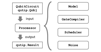
In this section, we describe the architecture of the simulation framework. The framework aims at simplifying the simulation of noisy quantum circuits through the explicit time evolution of physical qubits using QuTiP solvers. As illustrated in Figure 2, the simulation is designed around a Processor class, which consists of several different components. An instance of Processor emulates the behaviour of a quantum processor that takes a quantum circuit (QubitCircuit) as well as an initial quantum state (qutip.Qobj) and produces the final state as a (qutip.Result) object. As discussed further below in this section, the key improvements in the new qutip-qip package are the Model, GateCompiler, Scheduler and the Noise classes that allow a modular and flexible design of realistic quantum processors for simulations.
We illustrate our new framework here with an example simulating a 3-qubit Deutsch-Jozsa algorithm on a chain of spin qubits. We will work through this example and explain briefly the workflow and all the main modules. We then describe each module in detail in the subsequent subsections. The simulation of a more complicated circuit, a 10-qubit QFT algorithm, is presented in appendix B.
In qutip-qip, a quantum circuit is represented by an instance of the QubitCircuit class. The following code defines a circuit of a 3-qubit Deutsch-Jozsa algorithm (see Figure 3(a))333The code examples present in the main text and the Appendices are available at github.com/boxili/qutip-qip-paper. The code is compatible with qutip-qip==0.2.:
The Deutsch-Jozsa algorithm consists of an oracle constructed using two CNOT gates. The first two qubits in our circuit take a binary input and will be measured at the end while the last qubit is an ancillary qubit that stores the result of the oracle. The goal is to test if the oracle function is balanced or constant. A constant function returns all or for any input, while a balanced function returns for half of the input combinations and for the other half.
Among the four different classical inputs (), for half of them, the oracle returns 0 while for the other half it returns 1. Hence it is a balanced function and, without noise, the measurement of the first two qubits will never be both 0. One can run the gate-level simulation in the following way:
where we first initialize the state as using qutip.basis and then run the circuit simulation. By checking the final state, one will see that it has no overlap with or .
The above simulation is at the gate level and is computed by matrix-vector products of the gate operators and the input quantum state. We now describe how to simulate the circuit at the pulse level using Processor.
4.1 Processor
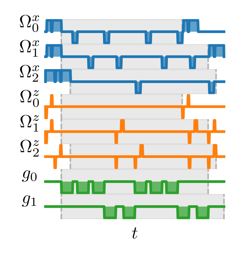
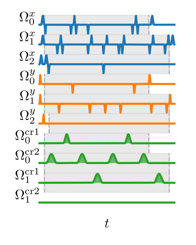
The Processor class handles the routine of a pulse-level simulation. It first compiles the circuit into a pulse-level description and then simulates the time evolution of the underlying physical system using QuTiP solvers. For different hardware models and compiling methods the same circuit can be compiled into different pulses, as shown in Figures 3(b), 3(c) and 3(d). Because of different noise models, the final state also differs from that of the ideal gate-level simulation.
In the following, we choose the spin chain model as an example for the underlying physical system and give an overview of the simulation procedure. We start from initializing a specific type of processor, a subclass of Processor called LinearSpinChain:
where we provide the number of qubits and the drive strength MHz. The other parameters, such as the interaction strength, are set to be the default value. The decoherence noise can also be added by specifying the coherence times ( and ) which we discuss hereafter.
By initializing this processor with the hardware parameters, a Hamiltonian model for a spin chain system is generated, including the drift and control Hamiltonians (, ). The Hamiltonian model is represented by the Model class and is saved as an attribute of the initialized processor. We provide different predefined models and discuss them more in Section 4.2. In addition, the Processor can also hold simulation configurations such as whether to use a cubic spline interpolation for the pulse coefficients. Such configurations are not directly part of the model but nevertheless could be important for the pulse-level simulation.
Next, we provide the circuit to the processor through the method load_circuit:
The processor will first decompose the gates in the circuit into native gates that can be implemented directly on the specified hardware model. Each gate in the circuit is then mapped to the control coefficients and driving Hamiltonians according to the GateCompiler defined for a specific model. A Scheduler is used to explore the possibility of executing several pulses in parallel. The compiler and scheduler classes will be explained in detail in Sections 4.3 and 4.4.
In addition to the standard compiler, optimal control algorithms in QuTiP can also be used to generate the pulses, which are implemented in OptPulseProcessor (Section 4.5).
With a pulse-level description of the circuit generated and saved in the processor, we can now run the simulation by
The run_state method first builds a Lindblad model including all the defined noise models (none in this example, but options are discussed below) and then calls a QuTiP solver to simulate the time evolution. One can pass solver parameters as keyword arguments to the method, e.g., tlist (time sequence for intermediate results), e_ops (measurement observables) and options (solver options). In the example above, we record the intermediate state at the time steps given by tlist. The returned result is a qutip.Result object, which, depending on the solver options, contains the final state, intermediate states and the expectation value. This allows one to extract all information that the solvers in QuTiP provide.
As for the simulation of noise, simple decoherence noise can be included in the Processor by specifying , e.g.,
More advanced noise models can be represented by the Noise class and added with the method Processor.add_noise. The following code is an equivalent way of defining a noise:
In general, the Noise class can be used to represent both decoherence and coherent noise sources. The former is defined by time-dependent or independent collapse operators and the latter by additional Hamiltonian terms in Eq. 2, with which distortion in the control coefficients or cross-talk can be represented. In particular, one can define noise that is correlated with the compiled ideal control coefficients through the Pulse class. They are explained in detail with examples in Sections 4.6 and 4.7.
Overall, the framework is designed in a modular way so that one can add custom Hamiltonian models, compilers and noise models. We describe in Section 4.8 how this can be done by defining new subclasses.
4.2 Model
The pulse-level simulation depends strongly on the modelling of the physical qubits. In the framework, the physical model is saved as an instance of the Model class in an initialized processor. A Model object contains the information regarding the specific quantum hardware, including the drift Hamiltonian that cannot be controlled, the available control Hamiltonians and possible noise in the system. A concrete physical model such as SpinChainModel is defined as a subclass of Model.
For convenience of use, a Model object is automatically generated while initializing a specific Processor, as in the example at the beginning of this section. To offer more flexibility, qutip-qip provides an equivalent way for the user to define a model and pass it to a Processor object, e.g.,
One can inquire about the properties of a control Hamiltonian through
which returns a tuple consisting of the Hamiltonian as a qutip.Qobj and the indices of the target qubits. For the predefined models, all available control Hamiltonians can be obtained by
The same interface is also provided in Processor (e.g., Processor.get_control) for convenience.
In predefined models, these control Hamiltonian terms are simply defined in a dictionary, equivalent to the following code:
which will be accessed by the model object. Notice that, in general, a model can be correctly recognized by the processor if the method Model.get_control(label) returns the results in the expected format, regardless of the internal implementation. For instance, in appendix C, we define it in a different way. This will be helpful, for instance, in an all-to-all connected system, e.g, using ions or neutral atoms, for which listing all the available combinations of target qubits is tedious.
Models allow one to simulate the physical qubits and their interaction in a more realistic way, e.g., using resonator-induced coupling and including leakage levels. This is demonstrated by a few predefined models that are implemented as subclasses of Model: the spin chain model, the qubits-resonator model and the fixed-frequency superconducting qubit model. Custom Hamiltonian models can be defined as subclasses as detailed in Sections 4.8 and C. In the following, we illustrate the characteristics of the predefined hardware models in detail.
4.2.1 Spin Chain model
The spin-exchange interaction exists in many quantum systems and is one of the earliest types of interaction used in quantum information processing, e.g., in Refs. [39, 40, 3]. Our predefined SpinChainModel implements a system of a few spin qubits with the exchange interaction arranged in a one-dimensional chain layout with either open ends or closed ends.
The interaction is only possible between adjacent qubits. For the spin model, the single-qubit control Hamiltonians are , , while the interaction is realized by the exchange Hamiltonian . The control Hamiltonian is given by
| (8) |
where , and are the time-dependent control coefficients and is the number of qubits.
4.2.2 Qubit-resonator model
In some experimental implementations, interactions are realized by a quantum bus or a resonator connecting different qubits. The qubit-resonator model describes a system composed of a single resonator and a few qubits connected to it. The coupling is kept small so that the resonator is rarely excited but acts only as a mediator for entanglement generation. The single-qubit control Hamiltonians used are and . The dynamics between the resonator and the qubits is captured by the Tavis-Cummings Hamiltonian, , where , are the destruction and creation operators of the resonator, while , are those of each qubit. The control of the qubit-resonator coupling depends on the physical implementation, but in the most general case we have single and multi-qubit control in the form,
| (9) |
In the numerical simulation, the resonator Hamiltonian is truncated to finite levels. The user can find a predefined CavityQEDModel implementing Eq. 9.
4.2.3 Superconducting qubit model
Superconducting-circuit qubits have been harnessed to provide artificial atoms for quantum simulation and quantum computing [3, 41, 42, 43, 44]. In our model, defined by the SCQubitsModel class, each qubit is simulated by a multi-level Duffing model, in which the qubit subspace is provided by the ground state and the first excited state. By default, the creation and annihilation operators are truncated at the third level, which can be adjusted, if desired, by the user. The multi-level representation can capture the leakage of the population out of the qubit subspace during single-qubit gates. The single-qubit control is generated by two orthogonal quadratures and . Same as the spin chain model, the interaction is possible only between adjacent qubits. Although this interaction is mediated by a resonator, for simplicity, we replace the complicated dynamics among two superconducting qubits and the resonator with a two-qubit effective Hamiltonian derived in [45].
As an example, we choose the cross resonance interaction in the form of , acting only on the two-qubit levels, which is widely used, e.g., in fixed-frequency superconducting qubits. We can write the Hamiltonian as
| (10) |
where the drift Hamiltonian is defined by the anharmonicity of the second excited state,
| (11) |
The coefficients and are computed from the qubit-resonator detuning and coupling strength [45]. With additional single-qubit gates, a CNOT gate can be realized using this type of interaction [46]. Using this effective Hamiltonian significantly reduces the size of the Hilbert space in the simulation and allows us to include more qubits. This flexibility in choosing different levels of detail in the modelling is one of the biggest advantages of this framework, in particular for noise simulation (as illustrated in more detail in Section 4.6).
4.3 Compiler
A compiler converts the quantum circuit to the corresponding pulse-level controls on the quantum hardware. In the framework, it is defined as an instance of the GateCompiler class. The compilation procedure is achieved through the following steps.
First, each quantum gate is decomposed into the native gates (e.g., rotation over , axes and the CNOT gate), using the existing decomposition scheme in QuTiP. If a gate acts on two qubits that are not physically connected, like in the chain model and superconducting qubit model, SWAP gates are added to match the topology before the decomposition. Currently, only 1-dimensional chain structures are supported.
Next, the compiler maps each quantum gate to a pulse-level control description. It takes the hardware parameter defined in the Hamiltonian model and computes the pulse duration and strength to implement the gate. For continuous pulses, the pulse shape can also be specified using SciPy window functions (scipy.signal.windows). A pulse scheduler is then used to explore the possibility of executing multiple quantum gates in parallel, which is explained in detail in Section 4.4.
In the end, the compiler returns a time-dependent pulse coefficient for each control Hamiltonian [see Eq. 2]. They contain the full information to implement the circuit and are saved in the processor. The coefficient is represented by two NumPy arrays, one for the control amplitude and the other for the time sequence. For a continuous pulse, a cubic spline is used to approximate the coefficient. This allows the use of compiled Cython code in QuTiP to achieve better performance.
For the predefined physical models described in the previous subsection, the corresponding compilers are also included and they will be used when calling the method Processor.load_circuit. As an example, we compile the three-qubit Deutsch-Jozsa algorithm, shown in Figure 3(a), while the compiled pulses on three different models are plotted in Figures 3(d), 3(b) and 3(c). From the plots, it is evident that the same circuit is compiled to completely different pulse-level controls:
-
•
For the spin chain model (Figure 3(b)), SWAP gates are added between and after the first CNOT gate, swapping the first two qubits (coefficient ). The SWAP gate is decomposed into three iSWAP gates, while the CNOT is decomposed into two iSWAP gates plus additional single-qubit corrections. Both the Hadamard gate and the two-qubit gates need to be decomposed to native gates (iSWAP and rotation on the and axes). The compiled coefficients are square pulses and the control coefficients on and are also different, resulting in different gate times.
-
•
For the superconducting-qubit processor (Figure 3(c)), the compiled pulses have a Gaussian shape. This is crucial for superconducting qubits because the second excited level is only slightly detuned from the qubit transition energy. A smooth pulse usually prevents leakage to the non-computational subspace. Similar to the spin chain, SWAP gates are added to switch the zeroth and first qubit and one SWAP gate is compiled to three CNOT gates. The control [defined in Eq. 10] is not used because there is no CNOT gate that is controlled by the second qubit and acts on the first one.
-
•
For the optimal control model (Figure 3(d)), we use the GRAPE algorithm, where control pulses are piece-wise constant functions. We provide the algorithm with the same control Hamiltonian model used for the spin chain model, Eq. (8). In the compiled optimal signals, all controls are active (non-zero pulse amplitude) during most of the execution time. We note that for identical gates on different qubits (e.g., Hadamard), each optimized pulse is different, demonstrating that the optimized solution is not unique, and there are further constraints one could apply, such as adaptions for the specific hardware.
As a demonstration of the capability of the simulator, we also compile a 10-qubit QFT algorithm using LinearSpinChain, as shown in appendix B.
To end this subsection, we mention that the gate decomposition is not fully optimized in QuTiP. Circuit optimization at the level of quantum gates, such as for an optimal number of two-qubit gates, depends on the hardware of interest and is still an open research topic [47, 48, 49, 50]. The same holds for mapping the circuit to the topology of the qubits’ connectivity [51, 52, 53]. Because the focus of this simulator is the simulation of the circuit at the physics level, we leave more advanced optimization and scheduling techniques at the gate level for future work. Instead, we offer the possibility to import quantum circuits defined in other libraries into QuTiP in the QASM format (see Section 5). This allows possible optimizations elsewhere and then exporting the optimized circuits in QuTiP for a pulse-level simulation.
4.4 Scheduler
The scheduling of a circuit consists of an important part of the compilation. Without it, the gates will be executed one by one and many qubits will be idling during the circuit execution, which increases the execution time and reduces the fidelity. In the framework, the scheduler is used after the control coefficient of each gate is computed. It runs a scheduling algorithm to determine the starting time of each gate while keeping the result correct.
The heuristic scheduling algorithm we provide offers two different modes: ASAP (as soon as possible) and ALAP (as late as possible). In addition, one can choose whether permutation among commuting gates is allowed to achieve a shorter execution time. The scheduler implemented here does not take the hardware architecture into consideration and assumes that the connectivity in the provided circuit matches with the hardware at this step.
In predefined processors, the scheduler runs automatically when loading a circuit and hence there is no action necessary from the side of the user. To help explain the scheduling algorithm, we provide here two examples of directly using the Scheduler class.
For gate scheduling, one can use
which, for the 3-qubit Deutsch-Jozsa example (Figure 3(a)), returns a list
This list denotes the gate cycle of each gate in the circuit. Here, all gates are assumed to have the same duration. One can see that that, e.g., the second CNOT and the last Hadamard on the first qubit are grouped together in cycle 3.
For pulse scheduling, one needs to use the Instruction class, which includes information about a specific implementation of a gate on the hardware, e.g., the duration of a gate. If we assume that all single-qubit gates take a time duration of 1 unit while the CNOT takes a time duration of 2 units, we can rewrite it as
Notice that now we used the ALAP scheduling. This returns a different list
with the starting time of each gate. In this result, the two CNOT gates (starting time 4 and 2) are exchanged, so that the first Hadamard on the zeroth qubit only needs to start at time step 3.
In the following, we describe our implementation of the pulse scheduler. The implementation is similar to Ref. [51, 54]. However, we omit the hardware-dependent part but allow gates to have different duration, generalizing it to a pulse scheduler. We focus on the ASAP scheduling while for the ALAP mode the circuit is reversed before it is passed to the algorithm and then reversed back after the scheduling.
We first represent the dependency among quantum gates in a quantum circuit as a directed acyclic graph. Each gate is represented by a node and the dependency by arrows. Gate A is considered dependent on gate B if A has to be executed after B. This also means that A needs to be executed after all the gates that B depends on. Hence, there is no loop in the graph. Next, all gates are divided into different cycles (ignoring the gate duration) according to the dependency graph. A priority is then assigned to each quantum gate, determined by the time required to execute all the gates that depend on it. The more time it takes to execute the gates after it, the higher priority is assigned to this gate. In the end, from the dependency graph and the priority, a list-scheduling algorithm is used to determine the order of the execution and the starting time of each operation.
Unlike scheduling classical gates, a scheduler of quantum gates needs to take the commutation relation into account. For instance, if two CNOT gates are controlled by the same qubit, but act on two different target qubits, they can be exchanged. Exploring this flexibility may reduce the total execution time, as shown in the example above. This is included in the process of building the dependency graph. All commuting gates are added to the same cycle when computing the priority and the one with the highest priority will be executed first. In general, more advanced techniques need to be applied to optimize the commuting gates, for instance as discussed in Ref. [54]. However, this becomes more complicated when gates have different execution times. For simplicity, we omit these advanced techniques in this implementation.
4.5 Optimal control
Apart from using compilers with predefined gate-to-pulse maps, one can also use the optimal control algorithm in QuTiP to find optimized control pulses. The algorithm can take arbitrary control Hamiltonians as input and uses quantum control function optimisation, based on open-loop quantum control theory [55] to find the best pulses. For a set of given control Hamiltonians , the optimal control module uses classical algorithms to optimize the control function in Eq. 2. Parameters of control pulses for realizing individual gates, sequences and hence complete circuits, are generated automatically through multi-variable optimization targeting maximum fidelity with the evolution described by the circuit.
The optimal control module in QuTiP supports both the GRAPE [23, 56] and the CRAB algorithms [57, 58]. The interface to use these algorithms in qutip-qip is implemented via the OptPulseProcessor class. One first provides the available control Hamiltonians that characterize the physical controls on the system, which, e.g., can be provided as an instance of the Model class, such as the SpinChainModel. Upon loading the quantum circuit, each quantum gate is expanded to a unitary acting on the full Hilbert space and passed to the optimal control algorithm as the desired target. The returned pulses that drive this are concatenated to complete a full circuit simulation of the physical control sequences. An example of optimized pulses is shown in Figure 3(d) and the code can be found in appendix A.
4.6 Noise
The noise module allows one to add control and decoherence noise following the Lindblad description of open quantum systems [Eq. 5]. Compared to the gate-based simulator (Section 3.1), this provides a more practical and straightforward way to describe the noise. In the current framework, noise can be added at different layers of the simulation, allowing one to focus on the dynamics of the dominant noise, while representing other noise, such as single-qubit relaxation, as collapse operators for efficiency. Depending on the problem studied, one can devote the computing resources to the most relevant type of noise.
Apart from imperfections in the Hamiltonian model and circuit compilation, the Noise class in the current framework defines deviations of the real physical dynamics from the compiled one. It takes the compiled pulse-level description of the circuit (see also Section 4.7) and adds noise elements to it, which allows defining noise that is correlated to the compiled pulses. In the following, we detail the three different noise models already available in the current framework.
Noise in the hardware model.
The Hamiltonian model defined in the Model class may contain intrinsic imperfections of the system and hence the compiled ideal pulse does not implement the ideal unitary gate. Therefore, building a realistic Hamiltonian model usually already introduces noise to the simulation. An example is the superconducting-qubit processor model (Section 4.2.3), where the physical qubit is represented by a multi-level system. Since the second excitation level is only weakly detuned from the qubit transition frequency, the population may leak out of the qubit subspace. Another example is an always-on ZZ type cross-talk induced by interaction with higher levels of the physical qubits [59], which is also implemented for the superconducting qubit model.
Control noise.
The control noise, as the name suggests, arises from imperfect control of the quantum system, such as distortion in the pulse amplitude or frequency drift. The simplest example is the random amplitude noise on the control coefficient in Eq. 2.
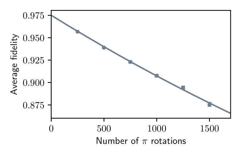
As a demonstration of control noise, we simulate classical cross-talk-induced decoherence between two neighbouring ion trap qubits described in [60]. We build a two-qubit Processor, where the second qubit is detuned from the first one by MHz. A sequence of -pulses with Rabi frequency of KHz and random phases are applied to the first qubit. We define noise such that the same pulse also applies to the second qubit. Because of the detuning, this pulse does not flip the second qubit but subjects it to a diffusive behaviour, so that the average fidelity of the second qubit with respect to the initial state decreases. This decreasing fidelity is shown experimentally in Figure 3a of Ref. [60].
Here, we reproduce these results with our two-qubit Processor in Figure 4. We start with an initial state of fidelity 0.975 and simulate the Hamiltonian
| (12) |
where is the ratio between the cross-talk pulse’s amplitudes. The plot in Figure 4 shows a similar fidelity decay curve as the experimental result, but includes only the contribution of cross-talk, while in the experimental result other noise sources may exist. This kind of simulation provides a way to identify noise contributions from different sources. The code is described in detail in appendix C, as an example of a custom noise model.
Lindblad noise.
The Lindblad noise originates from the coupling of the quantum system with the environment (e.g., a thermal bath) and leads to loss of information. It is simulated by collapse operators and results in non-unitary dynamics [34, 35].
The most commonly used type of Lindblad noise is decoherence, characterized by the coherence time and (dephasing). For the sake of convenience, one only needs to provide the parameter t1, t2 to the processor and the corresponding operators will be generated automatically. Both can be either a number that specifies one coherence time for all qubits or a list of numbers, each corresponding to one qubit.
For , the operator is defined as with as the destruction operator. For , the operator is defined as , where is the pure dephasing time given by . In the case of qubits, i.e., a two-level system, the destruction operator is truncated to a two-level operator and is consistent with Eq. 5. Constant and can be provided directly when initializing the Processor. Custom collapse operators, including time-dependent ones, can be defined through DecoherenceNoise. For instance, the following code defines a collapse operator using qutip.sigmam() and increases linearly as time:
Similar to the control noise, the Lindblad noise can also depend on the control coefficient.
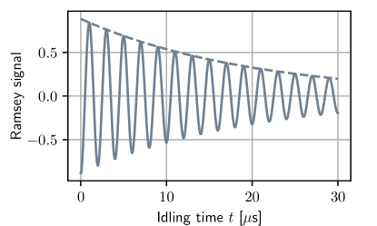
In order to demonstrate the simulation of decoherence noise, we build an example that simulates a Ramsey experiment as a quantum circuit run on a noisy Processor. The Ramsey experiment consists of a qubit that is initialized in the excited state, undergoes a rotation around the axis, idles for a time , and is finally measured after another rotation:
In the above block, we use the linear spin chain processor just for its compiler and do not use any of its default Hamiltonians. Instead, we define an always-on drift Hamiltonian with frequency MHz, an on-resonant drive with an amplitude of MHz and the coherence time . For different idling time , we record the expectation value with respect to the observable , which is plotted in Figure 5 as the solid curve. As expected, the envelope follows an exponential decay characterized by (dashed curve). Notice that, because -pulses are simulated as a physical process, the fitted decay does not start from 1. This demonstrates a way to include state preparation error into the simulation.
4.7 Pulse
As discussed before, in this simulation framework, we compile the circuit into pulse-level controls [Eq. 2] and simulate the time evolution of the physical qubits. In this subsection, we describe how the dynamics is represented internally in the workflow of qutip-qip, which is useful for understanding the simulation process as well as defining custom pulse-dependent noise.
A control pulse, together with the noise associated with it, is represented by a class instance of Pulse. When an ideal control is compiled and returned to the processor, it is saved as an initialized Pulse object, equivalent to the following code:
This code defines a -pulse implemented using the term in the Hamiltonian that flips the zeroth qubit specified by the argument targets. The pulse needs to be applied for the duration specified by the variable tlist. The parameters coeff and tlist together describe the control coefficient . Together with the provided Hamiltonian and target qubits, an instance of Pulse determines the dynamics of one control term.
With a Pulse initialized with the ideal control, one can define several types of noise, including the Lindblad or control noise as described in Section 4.6. An example of adding a noisy Hamiltonian as control noise through the method add_control_noise is given below:
The above code snippet adds a Hamiltonian term , which can, for instance, be interpreted as a frequency drift. Similarly, collapse operators depending on a specific control pulse can be added by the method Pulse.add_lindblad_noise.
In addition to a constant pulse, the control pulse and noise can also be provided as continuous functions. In this case, both tlist and coeff are given as NumPy arrays and a cubic spline is used to interpolate the continuous pulse coefficient. This allows using the compiled Cython version of the QuTiP solvers that have a much better performance than using a Python function for the coefficient. The option is provided as a keyword argument spline_kind="cubic" when initializing Pulse. Similarly, the interpolation method can also be defined for Processor using the same signature.
4.8 Adding custom hardware models
As it is impractical to include every physical platform, we provide an interface that allows one to customize the simulators. In particular, the modular architecture allows one to conveniently overwrite existing modules for customization.
To define a customized hardware model, the minimal requirements are a set of available control Hamiltonians , and a compiler, i.e., the mapping between native gates and control coefficients . One can either modify an existing subclass or write one from scratch by creating a subclass of the two parent classes Model and GateCompiler. Since different subclasses share the same interface, different models and compilers can also be combined to build new processors.
Moreover, this customization is not limited to Hamiltonian models and compiler routines. In principle, measurement can be defined as a customized quantum gate and the measurement statistics can be extracted from the obtained density matrix. A new type of noise can also be implemented by defining a new Noise subclass, which takes the compiled ideal Pulse and adds noisy dynamics on top of it.
An example of building a customized Model and GateCompiler, with custom types of noise, is provided in appendix C.
5 Importing and exporting circuits in QASM format
As pointed out in Section 4.3, it is impractical to include all the advanced techniques for circuit optimization and scheduling. To allow integration with other packages, we support import and export of circuits in the intermediate Quantum Assembly Language (QASM) format [31]. While there are different intermediate representations for quantum programs, and more specifically quantum circuits, including cQASM [61], qutip-qip provides support for OpenQASM. OpenQASM is an imperative programming language that can be used to describe quantum circuits in a back-end agnostic manner.
QuTiP includes a module to import and export quantum circuits compatible with the OpenQASM 2.0 standard [31]. OpenQASM 2.0 allows concise quantum circuit definitions including useful features like custom unitaries and defining groups of qubits over which a common gate can be applied simultaneously. Due to compatibility with multiple libraries such as Qiskit and Cirq, it is an easy way to transfer quantum circuits between these libraries and qutip-qip.
As an example, we use again the -qubit Deutsch-Jozsa circuit (Figure 3(a)). The following block defines the same circuit in the QASM format:
It can be saved as a .qasm file (such as ‘‘deutsch-jozsa.qasm’’ in our example below).
Every QASM file imported to qutip-qip requires the two header statements at the beginning of the file. The line OPENQASM 2.0 declares that the file adheres to the OpenQASM 2.0 standard. The keyword include processes a file that contains definitions of some QASM gates. It is available in the OpenQASM repository (as a standard file) and is included with the QASM file exported by qutip-qip (and also by Qiskit/Cirq). This circuit can be easily imported into qutip-qip using the read_qasm method in the following manner:
Furthermore, using the strmode option for read_qasm function, we can import the circuit described in a string object. Once a quantum circuit is defined, we can also export it to the QASM format and save it as a file using the save_qasm method:
The circuit can then be simulated with other packages. It is also possible to output the circuit as a string using circuit_to_qasm_str or print it out using print_qasm.
6 Conclusion
In this work, we presented a framework for pulse-level quantum circuit simulation that can be used to study noisy quantum devices simulated on classical computers. This framework builds on existing solvers and the quantum circuit model offered by QuTiP. We expanded the noise modeling capabilities with ad-hoc features for the simulation of controls in noisy quantum circuits, such as providing the option to inject coherent noise in pulses.
We provided a few predefined quantum hardware models, compiling and scheduling routines, as well as noise models, which can be adjusted to devote limited computing resources to the most relevant physical dynamics during the study of noise. We showed the simulation capabilities by illustrating how results obtained on cross-talk noise characterization for an ion-trap-based quantum processor can be easily replicated with this toolbox. Moreover, we provided an example of the simulation of Lindblad noise for a Ramsey experiment.
Due to the modular design, the framework introduced here can be integrated with more hardware models, gate decomposition and optimization schemes. In particular, the simulation of processors supporting bosonic models for quantum information processing, including quantum error correction schemes, is especially suitable within the current framework. Represented as customized gates, state preparation and measurement can also be simulated as a noisy physical process.
Pulse-level simulation could be helpful in quick verification of experimental results, developing quantum algorithms, such as variational quantum algorithms [62, 63, 4, 64], and testing compiling and scheduling schemes [53] with realistic noise models [65]. Through hardware simulation and noise simulation, quantum error correction code and quantum mitigation protocols can also be studied, for example, simulating pulse-level and digital zero-noise extrapolation [66, 67, 68].
Moreover, the noise characterization in model devices [69] and the impact of non-Markovian types of noise could be further evaluated [70, 21]. Future development in QuTiP aims at providing a unified interface to the open system solvers, which would enable a simpler integration with qutip-qip. This approach also has a potential to be integrated with other quantum control software such as qupulse [71] and C3 [72]. In particular, the features here introduced may be a useful tool to investigate from a novel perspective many-body dynamical properties of quantum circuits, such as for measurement-induced phase transitions [73], chaotic dynamics and information scrambling [74].
Planned developments in qutip and qutip-qip will enable the use of alternative quantum control optimization algorithms, that is options other than the GRAPE and CRAB algorithms that are currently supported. Most immediately Krotov-type algorithm support could be added through integration with qucontrol-krotov [19], which is already closely aligned with QuTiP. Further opportunities for development and integration with the main QuTiP package include the development of an implementation of the GOAT algorithm [75], in which qutip’s solvers of various kinds can be used effectively. This could then also be available for optimization of circuit controls to simulate universal gate operations [76, 77].
Another direction of development is the integration with other software frameworks, in the ecosystem of quantum open source software, where considerable duplication exists. Even with respect to the quantum intermediate representation of quantum circuits, standards are not yet solidified. For example, we have connected qutip-qip with OpenQASM 2.0, thus providing an access point to any major framework. More sophisticated features are expected in the upcoming OpenQASM 3.0 standard [32], including classical computation specifications and the option for pulse-level definitions for gates. Extending QuTiP support to OpenQASM 3.0 will be an important step in cross-package compatibility with respect to pulse-level quantum circuit simulation and their integration with real hardware.
The use of qutip-qip for open quantum hardware is an especially intriguing direction of research and development. One could envision this framework as the backbone for API inter-connectivity between simulation and hardware control in research labs with different technologies [71].
Acknowledgements
We would like to thank the whole community of contributors and users of the QuTiP project and in particular those who developed the quantum circuit representation in the qutip.qip module [30] – in particular Anubhav Vardhan, Robert Johansson, and Paul Nation. We also thank Jake Lishman, Èric Giguère, Purva Thakre and Simon Cross for work on the QuTiP project. We thank Andrea Mari, Anton Frisk Kockum, Daniel Burgarth, Sebastian Grijalva for useful discussions and comments on the manuscript. Part of this code development has been supported by NumFOCUS and Google Summer of Code. F. N. is supported in part by Nippon Telegraph and Telephone Corporation (NTT) Research, the Japan Science and Technology Agency (JST) [via the Quantum Leap Flagship Program (Q-LEAP), the Moonshot R&D Grant Number JPMJMS2061, and the Centers of Research Excellence in Science and Technology (CREST) Grant No. JPMJCR1676], the Japan Society for the Promotion of Science (JSPS) [via the Grants-in-Aid for Scientific Research (KAKENHI) Grant No. JP20H00134 and the JSPS–RFBR Grant No. JPJSBP120194828], the Army Research Office (ARO) (Grant No. W911NF-18-1-0358), the Asian Office of Aerospace Research and Development (AOARD) (via Grant No. FA2386-20-1-4069), and the Foundational Questions Institute Fund (FQXi) via Grant No. FQXi-IAF19-06. N. S. acknowledges partial support from the U.S. Department of Energy, Office of Science, Office of Advanced Scientific Computing Research, Accelerated Research in Quantum Computing under Award Number de-sc0020266. S. A. acknowledges support from the Knut and Alice Wallenberg Foundation through the Wallenberg Centre for Quantum Technology (WACQT).
Data availability
The code examples present in the main text and the Appendices are available at github.com/boxili/qutip-qip-paper. A version compatible with the latest distribution of qutip-qip can be found at github.com/qutip/qutip-qip.
Appendix A Simulating the Deutsch-Jozsa algorithm
In this section, we show the code example of simulating the 3-qubit Deutsch-Jozsa algorithm on three different hardware models: the spin chain model, the superconducting qubits, and the optimal control model:
In the above code block, we first define the Deutsch-Jozsa algorithm, same as the circuit shown in Figure 3(a). We then run the circuit on various hardware models. For the spin model and superconducting qubits, a Hamiltonian model and a compiler are already predefined and one only needs to load the circuit and run the simulation. Hardware parameters, such as the and times, qubit frequencies and coupling strength, can be given as parameters to initialize the processor. For optimal control, we use the control Hamiltonians of the spin chain model and provide a few parameters for the optimization routine in QuTiP, such as the maximal pulse amplitude and the number of time slots for each gate. For details, please refer to the QuTiP documentation (http://qutip.org/docs/latest/index.html).
The generated control pulses are shown in Figure 3(a) and can be obtained by the method:
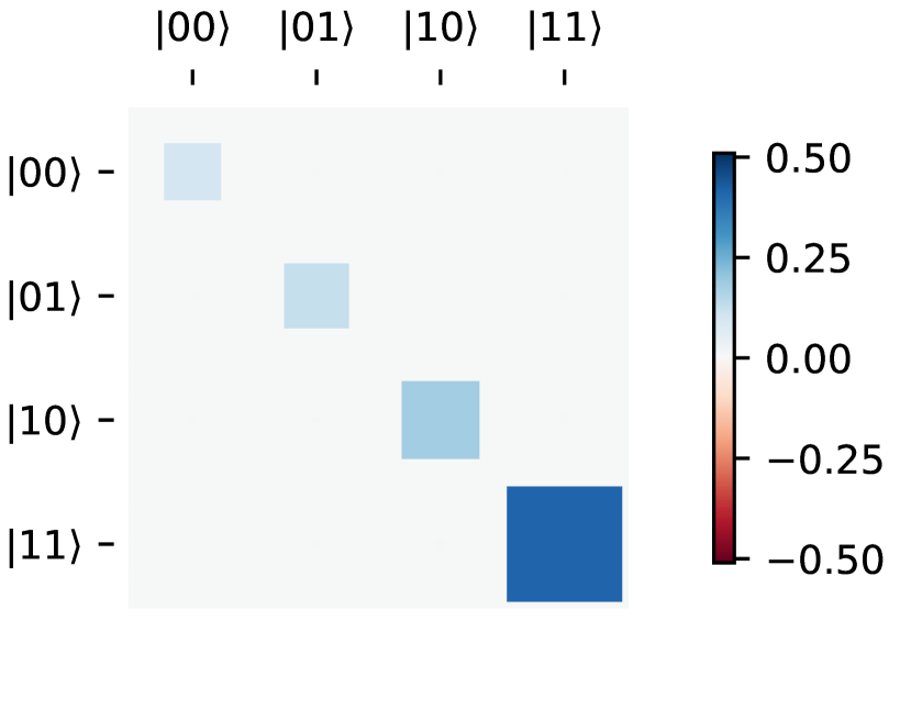
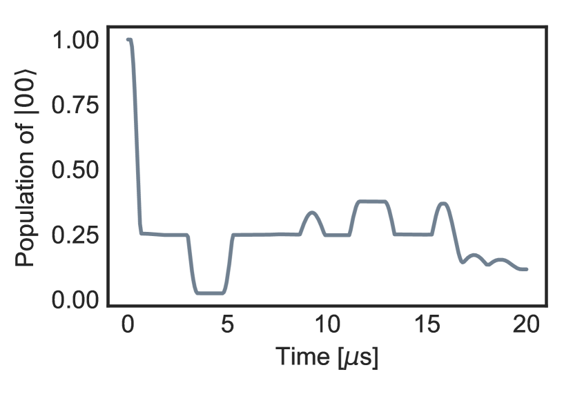
Because we are doing a simulation, we have access both to the final states as a density matrix and the information of the states during the evolution. We demonstrate this in Figure 6. By construction, the measured result of the first two qubits of a perfect Deutsch-Jozsa algorithm with a balanced oracle should not overlap with the state . This agrees with the small population of the state in the Hinton diagram (Figure 6(a)). The population is not exactly zero because we define a decoherence noise. In addition, we can also extract information during the circuit execution, e.g., the population as a function of time (Figure 6(b)).
Appendix B Compiling and simulating a 10-qubit Quantum Fourier Transform (QFT)
In this section, we simulate a 10-qubit Quantum Fourier Transform (QFT) algorithm. The QFT algorithm is one of the most important quantum algorithms in quantum computing [2]. It is, for instance, part of the Shor algorithm for integer factorization. The following code defines a 10-qubit QFT algorithm using CNOT and single qubit rotations and runs the simulation both at the gate level and at the pulse level.
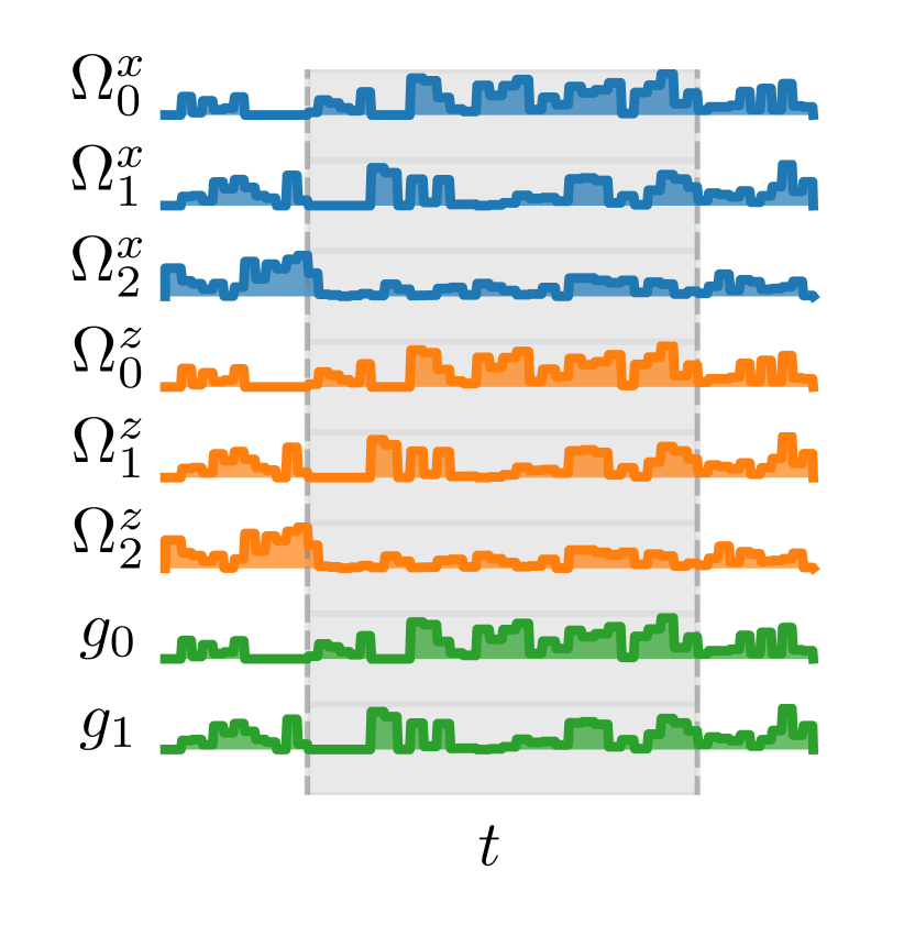
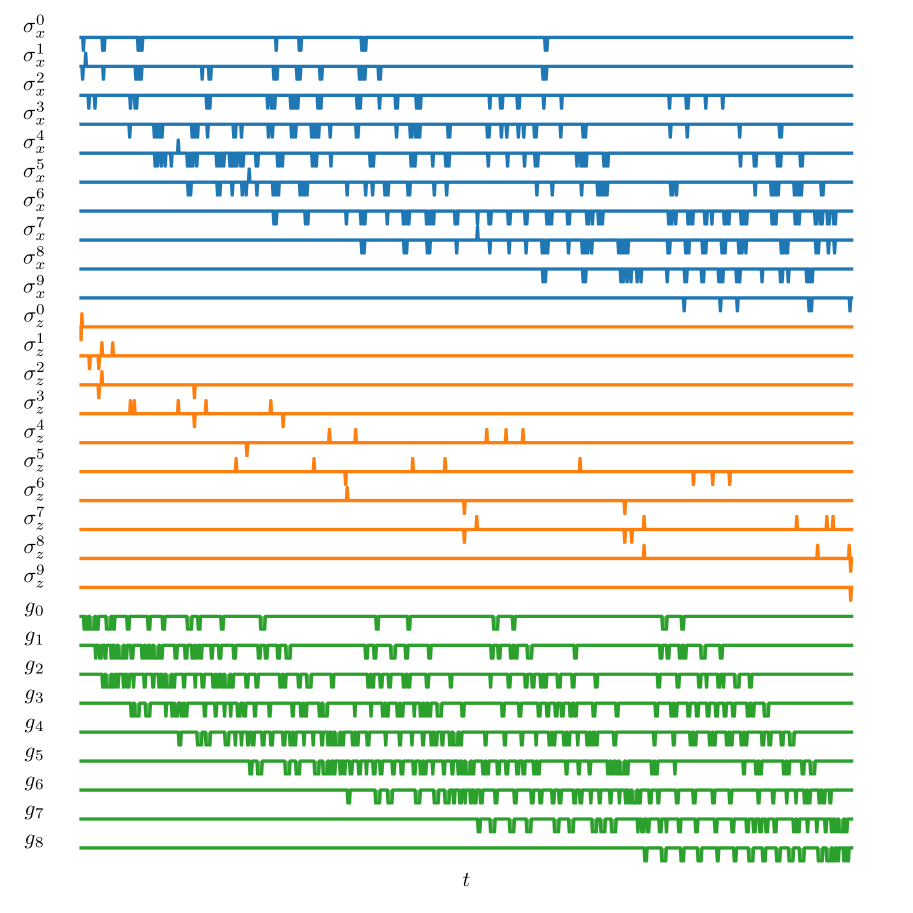
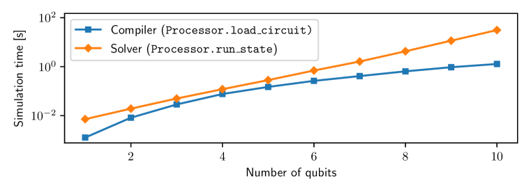
We plot the compiled pulses and perform a study of the simulation time in the top and bottom panels of Figure 7, respectively. The top panel of Figure 7 shows the control pulses (blue curves), (orange curves) and (green curves) for the spin chain model processor (Section 4.2), where counts the qubits. The pulses plotted implement the QFT algorithm represented in the native gates of the spin chain model, with single-qubit gates marked by rotations over the - and -axes and the iSWAP gate implemented through the spin-spin exchange interaction, marked by . While the sign for single-qubit drive denotes the phase of the control pulse, the negative sign in the coupling strengths is only a result of the convention used in the definition of the interaction, defined in Eq. 8.
In the bottom panel of Figure 7, we study the time it takes to simulate the dynamics for the QFT algorithm on the spin chain processor, from 1 to 10 qubits. We divide the simulation between compilation and solution of the dynamical equation. The compilation of the algorithm (blue squares in the bottom panel of Figure 7) includes native-gate gate decomposition, scheduling, and mapping to control pulses (as shown in the top panel). For 10 qubits, the compilation takes about one second, whereas the overall simulation time takes about half a minute on a commercial CPU (Intel i7 8700 with Max Turbo Frequency 4.60 GHz) with a single thread. Indeed, the overall simulation time is dominated by the task of solving the Schrödinger equation: this increases linearly with the circuit depth and exponentially with the size of the Hilbert space (orange diamonds in the bottom panel of Figure 7). The proportion of time used for the compilation with respect to the total simulation time decreases as the number of qubits in the QFT algorithm grows. As expected, we find that the bottleneck for the simulation of larger processors lies in the solution of the dynamics.
Note that, because of the pulse-level nature of the simulation, the overall simulation time also depends on the typical frequency characterizing the dynamics. In the above simulation, the maximum frequency in the Hamiltonian is about 1 MHz while the time scale of the quantum circuit is about 2 ms. No collapse operators are included. The simulation time may increase if decay or high-frequency coherent noise are included.
Appendix C Customizing the physical model and noise
In the following, we show a minimal example of constructing Hamiltonian models and compilers:
In this example, we first build a Hamiltonian model called MyModel. For simplicity, we only include two single-qubit control Hamiltonians: and . We then define the compiling routines for the two types of rotation gates RX and RY. In addition, we also define a rotation gate with mixed X and Y quadrature, parameterized by a phase , . This will be used later in the example of custom noise.
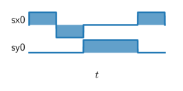
We then initialize a ModelProcessor with this model. In the ModelProcessor, the default simulation workflow is already defined, such as the load_circuit method. Since rotations around the and axes are the native gates of our hardware, we define them in the attribute native_gates. Providing this native gates set, rotation around axis will be automatically decomposed into rotations around and axes. We define a circuit consisting of rotation followed by a Z gate. The compiled pulses are shown in Figure 8, where the Z gate is decomposed into rotations around and axes.
Next, we show an example of defining customized noise and simulating classical cross-talk:
In the code block above, we first define a custom ClassicalCrossTalk noise object that uses the Noise class as the base. The get_noisy_dynamics method will be called during the simulation to generate the noisy Hamiltonian model. Here, we define a noise model that adds the same driving Hamiltonian to its neighbouring qubits, with a strength proportional to the control pulses strength applied on it. The detuning of the qubit transition frequency is simulated by adding a drift Hamiltonian to the processor, with a frequency of MHz.
Second, we define a random circuit consisting of a sequence of rotation pulses with random phases. The driving pulse is a pulse with a duration of and Rabi frequency KHz. As described in [60], this randomized benchmarking protocol allows one to study the classical cross-talk induced decoherence on the neighbouring qubits. The two qubits are initialized in the state with a fidelity of 0.975. After the circuit, we measure the population of the second qubit. If there is no cross-talk, it will remain perfectly in the ground state. However, cross-talk induces a diffusive behaviour of the second qubit and the fidelity decreases. This simulation is repeated 1600 times to obtain the average fidelity, as shown in Figure 4 in the main text.
References
- Preskill [2018] J. Preskill, Quantum computing in the NISQ era and beyond, Quantum 2, 79 (2018).
- Nielsen and Chuang [2000] M. A. Nielsen and I. L. Chuang, Quantum Computation and Quantum Information (Cambridge University Press, 2000).
- Buluta et al. [2011] I. Buluta, S. Ashhab, and F. Nori, Natural and artificial atoms for quantum computation, Rep. Prog. Phys. 74, 104401 (2011).
- Bharti et al. [2021] K. Bharti, A. Cervera-Lierta, T. H. Kyaw, T. Haug, S. Alperin-Lea, A. Anand, M. Degroote, H. Heimonen, J. S. Kottmann, T. Menke, W.-K. Mok, S. Sim, L.-C. Kwek, and A. Aspuru-Guzik, Noisy intermediate-scale quantum (NISQ) algorithms, arXiv preprint (2021), arXiv:2101.08448.
- Smith et al. [2016] R. S. Smith, M. J. Curtis, and W. J. Zeng, A Practical Quantum Instruction Set Architecture, arXiv preprint (2016), arXiv:1608.03355.
- Karalekas et al. [2020] P. J. Karalekas, N. A. Tezak, E. C. Peterson, C. A. Ryan, M. P. da Silva, and R. S. Smith, A quantum-classical cloud platform optimized for variational hybrid algorithms, Quantum Sci. Technol. 5, 024003 (2020).
- Aleksandrowicz et al. [2019] G. Aleksandrowicz, T. Alexander, P. Barkoutsos, L. Bello, Y. Ben-Haim, D. Bucher, F. J. Cabrera-Hernández, J. Carballo-Franquis, A. Chen, C.-F. Chen, J. M. Chow, et al., Qiskit: An Open-source Framework for Quantum Computing (2019).
- Developers [2021] C. Developers, Cirq (2021), See full list of authors on Github: https://github.com/quantumlib/Cirq/graphs/contributors.
- Steiger et al. [2018] D. S. Steiger, T. Häner, and M. Troyer, ProjectQ: an open source software framework for quantum computing, Quantum 2, 49 (2018).
- Bergholm et al. [2018] V. Bergholm, J. Izaac, M. Schuld, C. Gogolin, M. S. Alam, S. Ahmed, J. M. Arrazola, C. Blank, A. Delgado, S. Jahangiri, et al., PennyLane: Automatic differentiation of hybrid quantum-classical computations, arXiv preprint (2018), arXiv:1811.04968.
- Fingerhuth et al. [2018] M. Fingerhuth, T. Babej, and P. Wittek, Open source software in quantum computing, PLOS ONE 13, e0208561 (2018).
- Heim et al. [2020] B. Heim, M. Soeken, S. Marshall, C. Granade, M. Roetteler, A. Geller, M. Troyer, and K. Svore, Quantum programming languages, Nat. Rev. Phys. 2, 709 (2020).
- Alexander et al. [2020] T. Alexander, N. Kanazawa, D. J. Egger, L. Capelluto, C. J. Wood, A. Javadi-Abhari, and D. C McKay, Qiskit pulse: Programming quantum computers through the cloud with pulses, Quantum Sci. Technol. 5, 044006 (2020).
- Ball et al. [2021] H. Ball, M. J. Biercuk, A. R. R. Carvalho, J. Chen, M. Hush, L. A. D. Castro, L. Li, P. J. Liebermann, H. J. Slatyer, C. Edmunds, V. Frey, C. Hempel, and A. Milne, Software tools for quantum control: improving quantum computer performance through noise and error suppression, Quantum Sci. Technol. 6, 044011 (2021).
- Silvério et al. [2021] H. Silvério, S. Grijalva, C. Dalyac, L. Leclerc, P. J. Karalekas, N. Shammah, M. Beji, L.-P. Henry, and L. Henriet, Pulser: An open-source package for the design of pulse sequences in programmable neutral-atom arrays, arXiv preprint (2021), arXiv:2104.15044.
- Johansson et al. [2012] J. R. Johansson, P. D. Nation, and F. Nori, QuTiP: An open-source python framework for the dynamics of open quantum systems, Comput. Phys. Commun. 183, 1760 (2012).
- Johansson et al. [2013] J. R. Johansson, P. D. Nation, and F. Nori, QuTiP 2: A Python framework for the dynamics of open quantum systems, Comput. Phys. Commun. 184, 1234 (2013).
- Shammah et al. [2018] N. Shammah, S. Ahmed, N. Lambert, S. De Liberato, and F. Nori, Open quantum systems with local and collective incoherent processes: Efficient numerical simulations using permutational invariance, Phys. Rev. A 98, 063815 (2018).
- Goerz et al. [2019] M. H. Goerz, D. Basilewitsch, F. Gago-Encinas, M. G. Krauss, K. P. Horn, D. M. Reich, and C. P. Koch, Krotov: A Python implementation of Krotov’s method for quantum optimal control, SciPost Phys. 7, 80 (2019).
- Lambert et al. [2019] N. Lambert, S. Ahmed, M. Cirio, and F. Nori, Modelling the ultra-strongly coupled spin-boson model with unphysical modes, Nat. Commun. 10, 3721 (2019).
- Lambert et al. [2020] N. Lambert, T. Raheja, S. Ahmed, A. Pitchford, and F. Nori, BoFiN-HEOM: A bosonic and fermionic numerical hierarchical-equations-of-motion library with applications in light-harvesting, quantum control, and single-molecule electronics, arXiv preprint (2020), arXiv:2010.10806.
- Teske and Bluhm [2021] J. D. Teske and H. Bluhm, qopt: An experiment-oriented qubit simulation and quantum optimal control package, in IEEE Int. Conf. Quantum Comput. Eng. (QCE) (2021) p. 441.
- Khaneja et al. [2005] N. Khaneja, T. Reiss, C. Kehlet, T. Schulte-Herbrüggen, and S. J. Glaser, Optimal control of coupled spin dynamics: Design of NMR pulse sequences by gradient ascent algorithms, J. Magn. Reson. 172, 296 (2005).
- Horn [2021] L. B.-V. Horn, sequencing-dev/sequencing: v1.1.3 (2021).
- Groszkowski and Koch [2021] P. Groszkowski and J. Koch, Scqubits: a Python package for superconducting qubits, Quantum 5, 583 (2021).
- Harris et al. [2020] C. R. Harris, K. J. Millman, S. J. van der Walt, R. Gommers, P. Virtanen, D. Cournapeau, E. Wieser, J. Taylor, S. Berg, N. J. Smith, et al., Array programming with NumPy, Nature 585, 357 (2020).
- Virtanen et al. [2020] P. Virtanen, R. Gommers, T. E. Oliphant, M. Haberland, T. Reddy, D. Cournapeau, E. Burovski, P. Peterson, W. Weckesser, J. Bright, et al., SciPy 1.0: fundamental algorithms for scientific computing in Python, Nat. Methods 17, 261 (2020).
- Hunter [2007] J. D. Hunter, Matplotlib: A 2D graphics environment, Comput. Sci. Eng. 9, 90 (2007).
- Behnel et al. [2011] S. Behnel, R. Bradshaw, C. Citro, L. Dalcin, D. S. Seljebotn, and K. Smith, Cython: The best of both worlds, Computing in Science & Engineering 13, 31 (2011).
- [30] The full list of qutip-qip contributors, https://github.com/qutip/qutip-qip/graphs/contributors.
- Cross et al. [2017] A. W. Cross, L. S. Bishop, J. A. Smolin, and J. M. Gambetta, Open Quantum Assembly Language, arXiv preprint (2017), arXiv:1707.03429.
- Cross et al. [2021] A. W. Cross, A. Javadi-Abhari, T. Alexander, N. de Beaudrap, L. S. Bishop, S. Heidel, C. A. Ryan, J. Smolin, J. M. Gambetta, and B. R. Johnson, OpenQASM 3: A broader and deeper quantum assembly language, arXiv preprint (2021), arXiv:2104.14722.
- Nguyen et al. [2020] T. Nguyen, A. Santana, T. Kharazi, D. Claudino, H. Finkel, and A. McCaskey, Extending C++ for Heterogeneous Quantum-Classical Computing, arXiv preprint (2020), arXiv:2010.03935.
- Breuer and Petruccione [2002] H.-P. Breuer and F. Petruccione, The theory of open quantum systems (Oxford University Press, 2002).
- Lidar [2019] D. A. Lidar, Lecture Notes on the Theory of Open Quantum Systems, arXiv preprint (2019), arXiv:1902.00967.
- Carmichael [2009] H. J. Carmichael, Statistical methods in quantum optics 2: Non-classical fields (Springer Science & Business Media, 2009).
- Minganti et al. [2016] F. Minganti, N. Bartolo, J. Lolli, W. Casteels, and C. Ciuti, Exact results for Schrödinger cats in driven-dissipative systems and their feedback control, Sci. Rep. 6, 26987 (2016).
- Tanimura and Kubo [1989] Y. Tanimura and R. Kubo, Time evolution of a quantum system in contact with a nearly Gaussian-Markoffian noise bath, J. Phys. Soc. Jpn. 58, 101 (1989).
- Loss and DiVincenzo [1998] D. Loss and D. P. DiVincenzo, Quantum computation with quantum dots, Phys. Rev. A 57, 120 (1998).
- Kane [1998] B. E. Kane, A silicon-based nuclear spin quantum computer, Nature 393, 133 (1998).
- Devoret and Schoelkopf [2013] M. H. Devoret and R. J. Schoelkopf, Superconducting circuits for quantum information: An outlook, Science 339, 1169 (2013).
- Krantz et al. [2019] P. Krantz, M. Kjaergaard, F. Yan, T. P. Orlando, S. Gustavsson, and W. D. Oliver, A quantum engineer’s guide to superconducting qubits, Appl. Phys. Rev. 6, 021318 (2019).
- Gu et al. [2017] X. Gu, A. F. Kockum, A. Miranowicz, Y.-X. Liu, and F. Nori, Microwave photonics with superconducting quantum circuits, Phys. Rep. 718-719, 1 (2017).
- Kockum and Nori [2019] A. F. Kockum and F. Nori, Quantum bits with Josephson junctions, in Fundamentals and Frontiers of the Josephson Effect, edited by F. Tafuri (Springer, 2019) p. 703.
- Magesan and Gambetta [2020] E. Magesan and J. M. Gambetta, Effective Hamiltonian models of the cross-resonance gate, Phys. Rev. A 101, 052308 (2020).
- Rigetti and Devoret [2010] C. Rigetti and M. Devoret, Fully microwave-tunable universal gates in superconducting qubits with linear couplings and fixed transition frequencies, Phys. Rev. B 81, 134507 (2010).
- Maslov et al. [2008] D. Maslov, G. Dueck, D. Miller, and C. Negrevergne, Quantum circuit simplification and level compaction, IEEE Trans. Comput. Des. Integr. Circuits Syst. 27, 436 (2008).
- Javadi-Abhari et al. [2015] A. Javadi-Abhari, S. Patil, D. Kudrow, J. Heckey, A. Lvov, F. T. Chong, and M. Martonosi, ScaffCC: Scalable compilation and analysis of quantum programs, Parallel Comput. 45, 2 (2015).
- Häner et al. [2018] T. Häner, D. S. Steiger, K. Svore, and M. Troyer, A software methodology for compiling quantum programs, Quantum Sci. Technol. 3, 020501 (2018).
- Fösel et al. [2021] T. Fösel, M. Y. Niu, F. Marquardt, and L. Li, Quantum circuit optimization with deep reinforcement learning, arXiv preprint (2021), arXiv:2103.07585.
- Metodi et al. [2006] T. S. Metodi, D. D. Thaker, A. W. Cross, F. T. Chong, and I. L. Chuang, Scheduling physical operations in a quantum information processor, in Quantum Information and Computation IV, edited by E. J. Donkor, A. R. Pirich, and H. E. Brandt (2006) p. 62440T.
- Sargaran and Mohammadzadeh [2019] S. Sargaran and N. Mohammadzadeh, SAQIP: A Scalable Architecture for Quantum Information Processors, ACM Trans. Archit. Code Optim. 16 (2019).
- Murali et al. [2019] P. Murali, J. M. Baker, A. Javadi-Abhari, F. T. Chong, and M. Martonosi, Noise-adaptive compiler mappings for noisy intermediate-scale quantum computers, in Proc. 24th Int. Conf. Archit. Support Program. Lang. Oper. Syst. (ACM, 2019) p. 1015.
- Guerreschi and Park [2018] G. G. Guerreschi and J. Park, Two-step approach to scheduling quantum circuits, Quantum Sci. Technol. 3, 045003 (2018).
- D’Alessandro [2007] D. D’Alessandro, Introduction to Quantum Control and Dynamics (Chapman & Hall/CRC, 2007).
- Machnes et al. [2011] S. Machnes, U. Sander, S. J. Glaser, P. de Fouquières, A. Gruslys, S. Schirmer, and T. Schulte-Herbrüggen, Comparing, optimizing, and benchmarking quantum-control algorithms in a unifying programming framework, Phys. Rev. A 84, 022305 (2011).
- Caneva et al. [2011] T. Caneva, T. Calarco, and S. Montangero, Chopped random-basis quantum optimization, Phys. Rev. A 84, 022326 (2011).
- Doria et al. [2011] P. Doria, T. Calarco, and S. Montangero, Optimal control technique for many-body quantum dynamics, Phys. Rev. Lett. 106, 190501 (2011).
- Mundada et al. [2019] P. Mundada, G. Zhang, T. Hazard, and A. Houck, Suppression of qubit crosstalk in a tunable coupling superconducting circuit, Phys. Rev. Appl. 12, 054023 (2019).
- Piltz et al. [2014] C. Piltz, T. Sriarunothai, A. Varón, and C. Wunderlich, A trapped-ion-based quantum byte with next-neighbour cross-talk, Nat. Commun. 5, 4679 (2014).
- Khammassi et al. [2018] N. Khammassi, G. G. Guerreschi, I. Ashraf, J. W. Hogaboam, C. G. Almudever, and K. Bertels, cqasm v1. 0: Towards a common quantum assembly language, arXiv preprint (2018), arXiv:1805.09607.
- Alam et al. [2020] M. Alam, A. Ash-Saki, and S. Ghosh, Accelerating quantum approximate optimization algorithm using machine learning, in 2020 Des. Autom. Test Eur. Conf. Exhib. (DATE) (2020) p. 686.
- Haug and Kim [2021] T. Haug and M. S. Kim, Optimal training of variational quantum algorithms without barren plateaus, arXiv preprint (2021), arXiv:2104.14543.
- Magann et al. [2021] A. B. Magann, C. Arenz, M. D. Grace, T.-S. Ho, R. L. Kosut, J. R. McClean, H. A. Rabitz, and M. Sarovar, From pulses to circuits and back again: A quantum optimal control perspective on variational quantum algorithms, PRX Quantum 2, 010101 (2021).
- Erik et al. [2021] Erik, L. Saldyt, Rob, tjproct, J. Gross, sserita, kmrudin, T. L. Scholten, colibri-coruscans, kevincyoung, msarovar, coreyostrove, jordanh6, D. Nadlinger, L. N. Maurer, pyIonControl, and R. Blume-Kohout, pyGSTio/pyGSTi: Version 0.9.10 (2021).
- Kandala et al. [2019] A. Kandala, K. Temme, A. D. Córcoles, A. Mezzacapo, J. M. Chow, and J. M. Gambetta, Error mitigation extends the computational reach of a noisy quantum processor, Nature 567, 491 (2019).
- Giurgica-Tiron et al. [2020] T. Giurgica-Tiron, Y. Hindy, R. LaRose, A. Mari, and W. J. Zeng, Digital zero noise extrapolation for quantum error mitigation, in IEEE Int. Conf. Quantum Comput. Eng. (QCE) (2020) p. 306.
- LaRose et al. [2021] R. LaRose, A. Mari, S. Kaiser, P. J. Karalekas, A. A. Alves, P. Czarnik, M. E. Mandouh, M. H. Gordon, Y. Hindy, A. Robertson, P. Thakre, N. Shammah, and W. J. Zeng, Mitiq: A software package for error mitigation on noisy quantum computers, arXiv preprint (2021), arXiv:2009.04417.
- Dahlhauser and Humble [2021] M. L. Dahlhauser and T. S. Humble, Modeling noisy quantum circuits using experimental characterization, Phys. Rev. A 103, 042603 (2021).
- Schultz et al. [2021] K. Schultz, G. Quiroz, P. Titum, and B. D. Clader, SchWARMA: A model-based approach for time-correlated noise in quantum circuits, Phys. Rev. Research 3, 033229 (2021).
- Humpohl et al. [2021] S. Humpohl, L. Prediger, pcerf, P. Bethke, A. Willmes, J. Bergmann, M. Meyer, P. Eendebak, E. Kammerloher, T. Hangleiter, qutech-lab, L. Lankes, m-kreutz, bpapajewski, and P. Eendebak, qutech/qupulse: qupulse 0.6 (2021).
- Wittler et al. [2021] N. Wittler, F. Roy, K. Pack, M. Werninghaus, A. S. Roy, D. J. Egger, S. Filipp, F. K. Wilhelm, and S. Machnes, Integrated Tool Set for Control, Calibration, and Characterization of Quantum Devices Applied to Superconducting Qubits, Phys. Rev. Appl. 15, 034080 (2021).
- Skinner et al. [2019] B. Skinner, J. Ruhman, and A. Nahum, Measurement-induced phase transitions in the dynamics of entanglement, Phys. Rev. X 9, 031009 (2019).
- Blok et al. [2021] M. S. Blok, V. V. Ramasesh, T. Schuster, K. O’Brien, J. M. Kreikebaum, D. Dahlen, A. Morvan, B. Yoshida, N. Y. Yao, and I. Siddiqi, Quantum information scrambling on a superconducting qutrit processor, Phys. Rev. X 11, 021010 (2021).
- Machnes et al. [2018] S. Machnes, E. Assémat, D. Tannor, and F. K. Wilhelm, Tunable, Flexible, and Efficient Optimization of Control Pulses for Practical Qubits, Phys. Rev. Lett. 120, 150401 (2018).
- Dong et al. [2015] D. Dong, C. Chen, B. Qi, I. R. Petersen, and F. Nori, Robust manipulation of superconducting qubits in the presence of fluctuations, Sci. Rep. 5, 7873 (2015).
- Dong et al. [2016] D. Dong, C. Wu, C. Chen, B. Qi, I. R. Petersen, and F. Nori, Learning robust pulses for generating universal quantum gates, Sci. Rep. 6, 36090 (2016).
