Power-Efficient Wireless Streaming of Multi-Quality Tiled 360 VR Video in MIMO-OFDMA Systems

Abstract

In this paper, we study the optimal wireless streaming of a multi-quality tiled 360 virtual reality (VR) video from a multi-antenna server to multiple single-antenna users in a multiple-input multiple-output (MIMO)-orthogonal frequency division multiple access (OFDMA) system. In the scenario without user transcoding, we jointly optimize beamforming and subcarrier, transmission power, and rate allocation to minimize the total transmission power. This problem is a challenging mixed discrete-continuous optimization problem. We obtain a globally optimal solution for small multicast groups, an asymptotically optimal solution for a large antenna array, and a suboptimal solution for the general case. In the scenario with user transcoding, we jointly optimize the quality level selection, beamforming, and subcarrier, transmission power, and rate allocation to minimize the weighted sum of the average total transmission power and the transcoding power. This problem is a two-timescale mixed discrete-continuous optimization problem, which is even more challenging than the problem for the scenario without user transcoding. We obtain a globally optimal solution for small multicast groups, an asymptotically optimal solution for a large antenna array, and a low-complexity suboptimal solution for the general case. Finally, numerical results demonstrate the significant gains of proposed solutions over the existing solutions.

I Introduction

A360 virtual reality (VR) video can be generated by capturing a scene of interest in all directions simultaneously with an omnidirectional camera [2]. It is predicted that the VR market will reach 87.97 billion USD by 2025 [3]. Transmitting a 360 VR video over wireless networks enables users to experience immersive environments without geographical or behavioral restrictions. As a 360 VR video has a much larger file size than a traditional video, streaming an entire 360 VR video brings a heavy burden to wireless networks[4, 5, 6]. When watching a 360 VR video, a user perceives it from only one viewing direction at any time, which corresponds to one part of the 360 VR video, known as field-of-view (FoV). The tiling technique is widely adopted to improve the transmission efficiency for 360 VR videos [7]. Specifically, a 360 VR video is divided into smaller rectangular segments of the same size, known as tiles. Transmitting the set of tiles covering each predicted FoV can reduce the required communication resources without reducing the quality of experience [2, 7]. In practice, users may have heterogeneous conditions (e.g., channel conditions, display resolutions of devices, etc.). Pre-encoding each tile into multiple representations with different quality levels allows bitrate (quality) adaptation according to a user’s condition. Therefore, wireless streaming of a multi-quality tiled 360 VR video has received growing interest.

Recently, [8, 9, 10] study optimal wireless streaming of a multi-quality tiled 360 VR video in single-user networks. Specifically, [8, 9, 10] optimize the quality level selection [8, 10] or transmission rate [9] to minimize the total distortion [8, 9], or total utility [10]. The proposed solutions for single-user networks in [8, 9, 10] are not applicable in multi-user networks, as optimal resource sharing among users with heterogeneous channel conditions is not considered. In several VR applications, such as VR gaming, VR military training, and VR sports [11, 12], a 360 VR video has to be transmitted to multiple users simultaneously. When a tile is required by multiple users concurrently, multicast opportunities can be utilized to improve transmission efficiency. In [13, 14, 15, 16, 17, 18, 19], the authors study the optimal wireless streaming of a multi-quality tiled 360 VR video to multiple users by exploiting multicast opportunities. In particular, in our previous works [13, 14], we optimize transmission resource allocation to minimize the average transmission power for given video quality requirements of all users and optimize the encoding rate of each tile to maximize the received video quality for a given transmission power budget. In [15, 16, 17, 18, 19], the authors focus on optimizing quality level selection for each tile. Specifically, in [15, 16, 17], the authors maximize the total utility of all users [15, 16] or minimize the distortion of video scenes [17], without considering any constraints on quality variation. Consequently, more multicast opportunities can be exploited to further improve transmission efficiency. Nevertheless, the obtained quality levels of adjacent tiles may vary significantly, leading to poor viewing experiences [15, 16, 17]. In [18], the authors impose some constraints on quality variation while maximizing the total utility of all users to address this issue. Although the restrictions on quality variation in [18] can alleviate quality variation in an FoV to a certain extent, they cannot guarantee quality smoothness and are less mathematically tractable. In [19], user transcoding is adopted to ensure that the quality levels of all received tiles in each FoV are identical when maximizing the total utility of all users.

Despite the fruitful research in the literature, the performance of wireless streaming of a tiled 360 VR video is still unsatisfactory. The results in [13, 14, 15, 16, 17, 18, 19] are all for single-antenna servers, which cannot exploit spatial degrees of freedom for effective resource utilization. The performance of wireless systems can be improved by deploying multiple antennas at a server and designing efficient beamformers. Among various multi-antenna technologies, MIMO-OFDMA is the dominant air interface for 5G broadband wireless communications, as it can provide more reliable communications at high speeds. For instance, in [20, 21, 22], the authors consider single-group multicast [20] and multi-group multicast [21, 22]. Specifically, in [20], the authors consider the optimization of beamforming and power allocation to maximize the minimum user data rate. In [21], the authors consider the subcarrier allocation and power allocation to maximize the sum rate. However, the solutions proposed in [20, 21] are heuristic and hence have no performance guarantee. [22] studies the optimization of beamforming to minimize the total transmission power. A stationary point of the beamforming design problem is obtained based on successive convex approximation. Note that in [22], messages on each subcarrier are associated with different beamforming vectors, resulting in a substantial increase in the number of variables and the computational complexity for solving the optimization problem.

This paper considers the optimal wireless streaming of a multi-quality tiled 360 VR video from one server to multiple users in a MIMO-OFDMA system in the scenarios without and with user transcoding. With more advanced physical layer techniques than those in [13, 14, 15, 17, 18, 19], we expect the stringent requirements for 360 VR video transmission to be better satisfied. Assume that the set of tiles to be transmitted to each user has been determined and each user’s quality requirement is given. The main contributions of this paper are summarized below.

• In the scenario without user transcoding, we exploit natural multicast opportunities and formulate the minimization of the total transmission power with respect to (w.r.t.) beamforming, subcarrier allocation, transmission power, and rate allocation as a multi-group multicast problem in the MIMO-OFDMA system. This problem is a challenging mixed discrete-continuous optimization problem. We obtain its optimal solutions for two special cases, namely, the case of small multicast groups (for different sets of tiles) and the case of a large antenna array, exploiting decomposition, continuous relaxation, and Karush-Kuhn-Tucker (KKT) conditions. We also obtain a suboptimal solution for the general case using continuous relaxation and difference of convex (DC) programming. Note that previous works studying multi-group multicast in MIMO-OFDMA systems do not investigate special cases in which optimal solutions can be obtained [21, 22]. Besides, the proposed multi-group multicast formulation with one beamforming vector for each subcarrier can achieve the same performance as the multi-group multicast formulation in [22] which has one beamforming vector for each user and each subcarrier, but yields a substantially lower computational complexity for the general case.

• In the scenario with user transcoding, a flexible tradeoff between computation and communications resource consumptions can be struck via exploiting transcoding-enabled multicast opportunities. We utilize natural multicast opportunities and transcoding-enabled multicast opportunities and minimize the weighted sum of the average total transmission power and the transcoding power by optimizing the quality level selection, beamforming, and subcarrier, transmission power, and rate allocation. This problem extends the multi-group multicast optimization in the scenario without user transcoding, and it is a more challenging two-timescale mixed optimization problem. For two special cases, we obtain the corresponding optimal solutions. For the general case, we obtain a low-complexity suboptimal solution. Note that the formulations in [21] and [22], which consider only natural multicast opportunities, cannot provide an effective design in the scenario with user transcoding.

• Finally, numerical results show substantial gains achieved by the proposed solutions over existing schemes and demonstrate the advantages of multicast and user transcoding in wireless streaming of a multi-quality tiled 360 VR video. Furthermore, numerical results illustrate that the proposed low-complexity optimal solution obtained for a large antenna array can achieve promising performance when the number of antennas is moderate, demonstrating its effectiveness.

Note that this work extends our previous results on wireless streaming of a multi-quality tiled 360 VR video in time division multiple access (TDMA) systems [13, 18, 19] and OFDMA systems [14]. The extensions are highly nontrivial due to the non-convexity w.r.t beamforming vectors. To the best of our knowledge, this is the first work providing an optimization-based design for wireless streaming of a multi-quality tiled 360 VR video in MIMO-OFDMA systems.

Notation: For a Hermitian matrix $\mathbf{A}$, $\mathbf{A}\succeq\mathbf{0}$ means that $\mathbf{A}$ is an Hermitian positive semidefinite matrix. The symbol $(\cdot)^{H}$ denotes complex conjugate transpose operator. $\text{tr}(\cdot)$ and $\text{rank}(\cdot)$ denote the trace and the rank, respectively. $\mathbb{E}[\cdot]$ denotes the statistical expectation. $\mathcal{CN}(\mathbf{a},\mathbf{R})$ represents the distribution of circularly-symmetric complex Gaussian random vectors with mean vector $\mathbf{a}$ and covariance matrix $\mathbf{R}$. $\mathbf{I}_{N}$ denotes the $N\times N$ identity matrix. $\mathbb{C}^{N\times M}$ denotes the space of $N\times M$ matrices with complex entries.

II System Model

Wireless streaming of a multi-quality tiled 360 VR video from a server (e.g., access point or base station) to multiple users arises in several VR applications such as VR gaming, VR concert, VR military training, and VR sports. This paper aims to optimize the wireless streaming of a multi-quality tiled 360 VR video from a server to $K$ users in a MIMO-OFDMA system as illustrated in Fig. 1. The server is equipped with $M$ transmit antennas and each user wears a single-antenna VR headset. Denote $\mathcal{K}\triangleq\{1,\ldots,K\}$ as the set of user indices. When a VR user is interested in one viewing direction of a 360 VR video, the user watches a rectangular FoV of size $F_{h}\times F_{v}$ (in rad$\times$rad), the center of which is referred to as the viewing direction. Besides, a user can freely switch views when watching a 360 VR video.

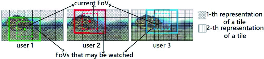
(a) Multi-quality tiled 360 VR video required by multiple users.

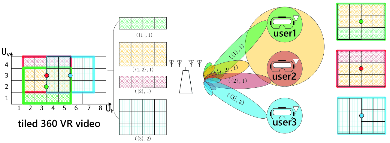
(b) Scenario without user transcoding.

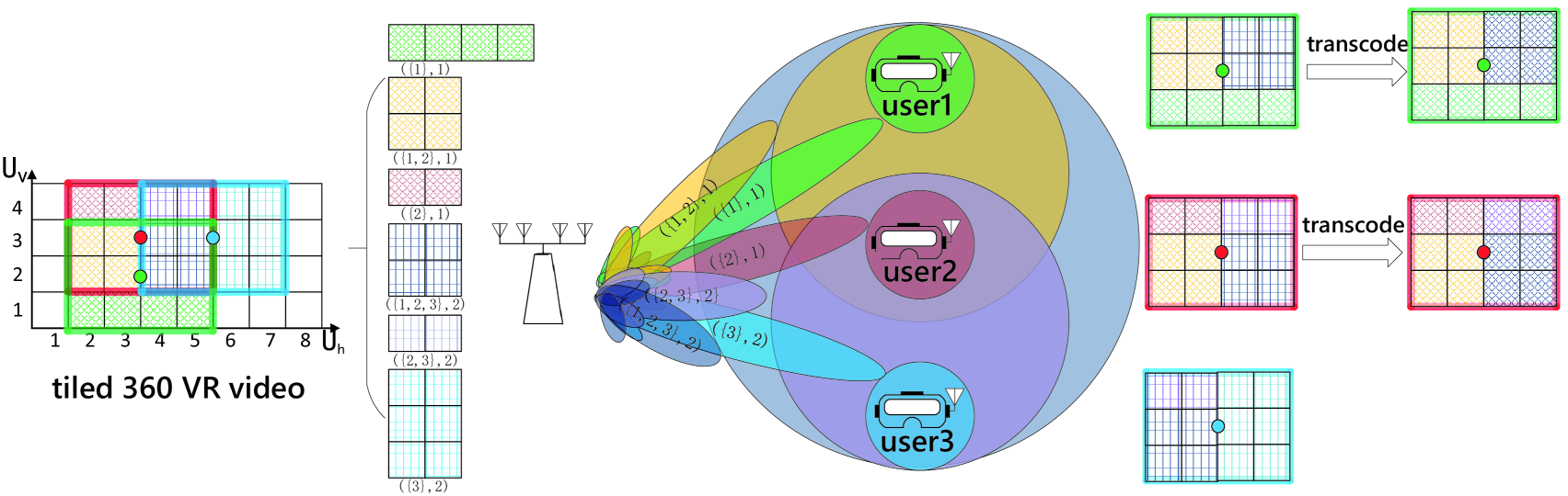
(c) Scenario with user transcoding.

Figure 1: System models of wireless streaming of a multi-quality tiled 360 VR video in the two scenarios. $K=3$, $\mathbf{r}=(1,1,2),$ $U_{h}\times U_{v}=8\times 4$, $M=4$, $\mathcal{G}_{1}=\{(2,1),(3,1),(4,1),(5,1),(2,2),(3,2),(4,2),(5,2),(2,3),(3,3),$ $(4,3),(5,3)\}$, $\mathcal{G}_{2}=\{(2,2),(3,2),(4,2),(5,2),(2,3),(3,3),(4,3)$, $(5,3),(2,4),$ $(3,4),(4,4),(5,4)\}$, $\mathcal{G}_{3}=\{(4,2),(5,2),(6,2),(7,2),(4,3),(5,3),$ $(4,4),(5,4),(6,4),(7,4)\}$, $\mathcal{I}=\{\{1\},\{2\},\{3\},\{1,3\},\{2,3\},\{1,2,3\}\}$, $\mathcal{P}_{\{1\}}=\{(2,1),(3,1),(4,1),(5,1)\}$, $\mathcal{P}_{\{2\}}=\{(2,4),(3,4)\}$, $\mathcal{P}_{\{3\}}=\{(6,2),(6,3),(6,4),(7,2),(7,3),(7,4)\}$, $\mathcal{P}_{\{1,2\}}=\{(2,2),(2,3),(3,2),(3,3)\}$, $\mathcal{P}_{\{2,3\}}=\{(4,4),(5,4)\}$, $\mathcal{P}_{\{1,2,3\}}=\{(4,2),(4,3),(5,2),(5,3)\}$, $\mathcal{K}_{\{1\},1}=\{1\},$ $\mathcal{K}_{\{1,2\},1}=\{1,2\},$ $\mathcal{K}_{\{2\},1}=\{2\},$ $\mathcal{K}_{\{3\},2}=\{3\}.$

Tiling is adopted to improve the transmission efficiency of the 360 VR video [7]. In particular, the 360 VR video is divided into $U_{h}\times U_{v}$ rectangular segments of the same size, referred to as tiles, where $U_{h}$ and $U_{v}$ represent the numbers of segments in each row and column, respectively. Define $\mathcal{U}_{h}\triangleq\{1,\ldots,U_{h}\}$ and $\mathcal{U}_{v}\triangleq\{1,\ldots,U_{v}\}$. The $(u_{h},u_{v})$-th tile corresponds to the tile in the $u_{h}$-th row and the $u_{v}$-th column, for all $u_{h}\in\mathcal{U}_{h}$ and $u_{v}\in\mathcal{U}_{v}$. Considering user heterogeneity (e.g., channel conditions, display resolutions of devices, etc.), each tile is pre-encoded into $L$ representations corresponding to $L$ quality levels using High Efficiency Video Coding (HEVC), as in Dynamic Adaptive Streaming over HTTP (DASH). Denote $\mathcal{L}\triangleq\{1,\ldots,L\}$ as the set of quality levels. For all $l\in\mathcal{L}$, the $l$-th representation of each tile corresponds to the $l$-th lowest quality. For ease of exposition, we assume that the encoding rates of the tiles with the same quality level are identical. Let $D_{l}$ (in bits/s) denote the encoding rate of the $l$-th representation of a tile. Note that $D_{1}<D_{2}<\ldots<D_{L}$. We study the system for the duration of the playback time of multiple groups of pictures (GOPs). In this duration, the FoV of each user does not change. Denote $r_{k}\in\mathcal{L}$ as the quality level for the FoV of user $k\in\mathcal{K}$. Because of the video coding structure, $\mathbf{r}\triangleq(r_{k})_{k\in\mathcal{K}}$ should not change during the considered time duration.

As in [13, 14, 18, 19], the server collects a user’s information such as head orientation (tracked by a 3DoF or 6DoF VR headset) and location (tracked by a 6DoF VR headset) from the user’s headset via the uplink transmission, predicts the user’s FoV and determines the set of tiles to be transmitted to the user. Denote $\mathcal{G}_{k}$ as the set of indices of the tiles that need to be transmitted to user $k$. Denote $\mathcal{G}\triangleq\bigcup_{k\in\mathcal{K}}\mathcal{G}_{k}$ as the set of indices of the tiles that need to be sent to all $K$ users. For all $\mathcal{S}\subseteq\mathcal{K}$, $\mathcal{S}\neq\emptyset$, denote $\mathcal{P}_{\mathcal{S}}\triangleq\left(\bigcap_{k\in\mathcal{S}}\mathcal{G}_{k}\right)\bigcap\left(\mathcal{G}-\bigcup_{k\in\mathcal{K}\setminus\mathcal{S}}\mathcal{G}_{k}\right)$ as the set of indices of the tiles that are needed by all users in $\mathcal{S}$ and are not needed by the users in $\mathcal{K}\setminus\mathcal{S}$. Then $\mathcal{P}\triangleq\{\mathcal{P}_{\mathcal{S}}|\mathcal{P}_{\mathcal{S}}\neq\emptyset,~{}\mathcal{S}\subseteq\mathcal{K},~{}\mathcal{S}\neq\emptyset\}$ forms a partition of $\mathcal{G}$ and $\mathcal{I}\triangleq\{\mathcal{S}|\mathcal{P}_{\mathcal{S}}\neq\emptyset,~{}\mathcal{S}\subseteq\mathcal{K},~{}\mathcal{S}\neq\emptyset\}$ specifies the user sets corresponding to the partition. Denote $I\triangleq|\mathcal{I}|$. Let $\mathcal{I}_{k}\triangleq\{\mathcal{S}|\mathcal{S}\subseteq\mathcal{I},k\in\mathcal{S}\}$, $k\in\mathcal{K}$. The tiles in $\mathcal{P}_{\mathcal{S}}$, $\mathcal{S}\in\mathcal{I}_{k}$ are required by user $k$. We consider the tiles in each set jointly rather than separately, to reduce the complexity for transmission and resource allocation. For all $l\in\mathcal{L}$ and $\mathcal{S}\subseteq\mathcal{K}$, the encoding (source coding) bits of the $l$-th representations of the tiles in $\mathcal{P}_{\mathcal{S}}$ are “aggregated” into one message indexed by $(\mathcal{S},l)$, which is transmitted at most once to the users in $\mathcal{S}$ that will utilize it, to improve transmission efficiency. For all $\mathcal{S}\in\mathcal{I}$ and $l\in\mathcal{L}$, let $\mathcal{K}_{\mathcal{S},l}\triangleq\{k\in\mathcal{S}|r_{k}=l\}$. If there is only one user in $\mathcal{K}_{\mathcal{S},l}$, the transmission of message $(\mathcal{S},l)$ corresponds to unicast; and if there are multiple users in $\mathcal{K}_{\mathcal{S},l}$, the transmission of message $(\mathcal{S},l)$ corresponds to multicast. Thus, the multi-quality tiled 360 VR video transmission to the $K$ users may involve both unicast and multicast. An illustration example can be seen in Fig. 1 (b).

Let $\mathcal{N}\triangleq\{1,\ldots,N\}$, where $N$ is the number of subcarriers. The bandwidth of each subcarrier is $B$ (in Hz). We assume block fading, i.e., the small-scale channel fading coefficients do not change within one frame. Let $\mathbf{H}_{n,k}\in\mathbb{C}^{M\times 1}$ denote the random small-scale fading coefficient between the server and user $k$ on subcarrier $n$. Denote $\mathbf{H}\triangleq(\mathbf{H}_{n,k})_{n\in\mathcal{N},k\in\mathcal{K}}$. Let $\mathbf{h}\triangleq(\mathbf{h}_{n,k})_{n\in\mathcal{N},k\in\mathcal{K}}$ represent a realization of $\mathbf{H}$ (which can be obtained by the server via channel estimation), where $\mathbf{h}_{n,k}\in\mathbb{C}^{M\times 1}$ is a realization of $\mathbf{H}_{n,k}$. Let $\beta_{k}>0$ denote the large-scale channel fading gain between the server and user $k$, which remains constant during the considered time duration and is known to the server.

Denote $\mu_{\mathcal{S},l,n}(\mathbf{h})\in\{0,1\}$ as the subcarrier assignment indicator for subcarrier $n$ and message $(\mathcal{S},l)$ under $\mathbf{h}$, where $\mu_{\mathcal{S},l,n}(\mathbf{h})=1$ indicates that subcarrier $n$ is assigned to transmit the symbols for message $(\mathcal{S},l)$, $\mu_{\mathcal{S},l,n}(\mathbf{h})=0$ otherwise. For ease of implementation, assume that each subcarrier is assigned to transmit symbols of only one message in each frame [23, 24]. Thus, subcarrier allocation constraints are given by

$$\mu_{\mathcal{S},l,n}(\mathbf{h})\in\{0,1\},~{}\mathcal{S}\in\mathcal{I},l\in\mathcal{L},n\in\mathcal{N},$$ (1)

$$\sum\nolimits_{\mathcal{S}\in\mathcal{I}}\sum\nolimits_{l\in\mathcal{L}}\mu_{\mathcal{S},l,n}(\mathbf{h})=1,~{}n\in\mathcal{N}.$$ (2)

To capture the scaling of the transmission power with $M$ for studying the optimal power allocation at large $M$, let $\frac{\eta_{\mathcal{S},l,n}(\mathbf{h})}{M}$ denote the transmission power for the symbols for message $(\mathcal{S},l)$ on subcarrier $n$ under $\mathbf{h}$, where

$$\eta_{\mathcal{S},l,n}(\mathbf{h})\geq 0,~{}\mathcal{S}\in\mathcal{I},l\in\mathcal{L},n\in\mathcal{N}.$$ (3)

The total transmission power is $\sum\limits_{n\in\mathcal{N}}\sum\limits_{\mathcal{S}\in\mathcal{I}}\sum\limits_{l\in\mathcal{L}}\frac{\mu_{\mathcal{S},l,n}(\mathbf{h})\eta_{\mathcal{S},l,n}(\mathbf{h})}{M}.$

Suppose that subcarrier $n$ is assigned to transmit the symbols for message $(\mathcal{S},l)$. Let $s_{\mathcal{S},l,n}$ represent the symbols for message $(\mathcal{S},l)$ transmitted on subcarrier $n$. Assume $\mathbb{E}[|s_{\mathcal{S},l,n}|^{2}]=1$ for all $l\in\mathcal{L},\mathcal{S}\in\mathcal{I}$ and $n\in\mathcal{N}$. Let $\mathbf{w}_{n}(\mathbf{h})\in\mathbb{C}^{M\times 1}$ denote the beamforming vector for the message transmitted on subcarrier $n$ under $\mathbf{h}$, where

$$\|\mathbf{w}_{n}(\mathbf{h})\|_{2}=1,~{}n\in\mathcal{N}.$$ (4)

The received signal at user $k$ on subcarrier $n$ is given by

$$y_{\mathcal{S},l,k,n}=\sqrt{\beta_{k}\frac{\eta_{\mathcal{S},l,n}(\mathbf{h})}{M}}\mathbf{h}_{n,k}^{H}\mathbf{w}_{n}(\mathbf{h})s_{\mathcal{S},l,n}+z_{n,k},~{}k\in\mathcal{K},n\in\mathcal{N},$$

where $z_{n,k}\sim\mathcal{CN}(0,\sigma^{2})$ represents the noise at user $k$ on subcarrier $n$. To obtain design insights, we consider the application of a capacity achieving code [23, 25, 26]. The maximum transmission rate for the symbols for message $(\mathcal{S},l)$ to user $k\in\mathcal{S}$ on subcarrier $n$ under $\mathbf{h}$ is given by $B\log_{2}\left(1+\frac{\eta_{\mathcal{S},l,n}(\mathbf{h})\beta_{k}|\mathbf{h}_{n,k}^{H}\mathbf{w}_{n}(\mathbf{h})|^{2}}{M\sigma^{2}}\right)$ (in bit/s). Let $c_{\mathcal{S},l,n}(\mathbf{h})$ denote the transmission rate for the symbols for message $(\mathcal{S},l)$ on subcarrier $n$ under $\mathbf{h}$, where

$$c_{\mathcal{S},l,n}(\mathbf{h})\geq 0,~{}\mathcal{S}\in\mathcal{I},l\in\mathcal{L},n\in\mathcal{N}.$$ (5)

Then, $\sum_{n\in\mathcal{N}}c_{\mathcal{S},l,n}$ represents the transmission rate of message $(\mathcal{S},l)$.

In Section III, we will consider the scenario where users cannot perform transcoding but directly play the received messages. In Section IV, we will consider the scenario where users can first perform transcoding, i.e., convert a tile representation at a certain quality level to a lower quality level using transcoding tools such as Fast Forward Mpeg (FFmpeg), and then play the received video.

III Total Transmission Power Minimization Without User Transcoding

In this section, we consider the scenario without user transcoding. For all $\mathcal{S}\in\mathcal{I}$, let $\mathcal{L}_{\mathcal{S}}\triangleq\{r_{k}|k\in\mathcal{S}\}$. When $|\mathcal{K}_{\mathcal{S},l}|>1$, message $(\mathcal{S},l)$, where $\mathcal{S}\in\mathcal{I}$ and $l\in\mathcal{L}_{\mathcal{S}}$ can be transmitted to all users in $\mathcal{K}_{\mathcal{S},l}$ simultaneously via multicast. This type of multicast opportunities are referred to as natural multicast opportunities [13, 14, 18, 19]. An illustration example is shown in Fig. 1 (b). In this example, by using natural multicast opportunities, the server multicasts message $(\{1,2\},1)$ to user 1 and user 2.

Consider one frame with small-scale fading coefficients $\mathbf{h}$. To guarantee that message $(\mathcal{S},l)$ can be successfully sent to each user $k\in\mathcal{K}_{\mathcal{S},l}$ on subcarrier $n$ under $\mathbf{h}$, we have

$$\mu_{\mathcal{S},l,n}(\mathbf{h})B\log_{2}\left(1+\frac{\eta_{\mathcal{S},l,n}(\mathbf{h})\beta_{k}|\mathbf{h}_{n,k}^{H}\mathbf{w}_{n}(\mathbf{h})|^{2}}{M\sigma^{2}}\right)$$

$$\geq c_{\mathcal{S},l,n}(\mathbf{h}),\mathcal{S}\in\mathcal{I},l\in\mathcal{L}_{\mathcal{S}},k\in\mathcal{K}_{\mathcal{S},l},n\in\mathcal{N}.$$ (6)

To maximally avoid rebuffering and reduce startup delay, we require that the transmission rate of each message $(\mathcal{S},l)$ is no smaller than its encoding rate

$$\sum\nolimits_{n\in\mathcal{N}}c_{\mathcal{S},l,n}(\mathbf{h})\geq|\mathcal{P}_{\mathcal{S}}|D_{l},~{}\mathcal{S}\in\mathcal{I},l\in\mathcal{L}_{\mathcal{S}},$$ (7)

where $|\mathcal{P}_{\mathcal{S}}|$ denotes the number of tiles in $\mathcal{P}_{\mathcal{S}}$.

For convenience, denote $\bm{\mu}(\mathbf{h})\triangleq(\mu_{\mathcal{S},l,n}(\mathbf{h}))_{\mathcal{S}\in\mathcal{I},l\in\mathcal{L}_{\mathcal{S}},n\in\mathcal{N}}$, $\bm{\eta}(\mathbf{h})\triangleq(\eta_{\mathcal{S},l,n}(\mathbf{h}))_{\mathcal{S}\in\mathcal{I},l\in\mathcal{L}_{\mathcal{S}},n\in\mathcal{N}}$, $\mathbf{c}(\mathbf{h})\triangleq(c_{\mathcal{S},l,n}(\mathbf{h}))_{\mathcal{S}\in\mathcal{I},l\in\mathcal{L}_{\mathcal{S}},n\in\mathcal{N}}$ and $\mathbf{w}(\mathbf{h})\triangleq(\mathbf{w}_{n}(\mathbf{h}))_{n\in\mathcal{N}}$. We consider $\bm{\mu}(\mathbf{h}),\bm{\eta}(\mathbf{h}),\mathbf{c}(\mathbf{h}),\mathbf{w}(\mathbf{h})$ as functions of $\mathbf{h}$, respectively. Given the quality levels of all users $\mathbf{r}$, we would like to optimize $\bm{\mu}(\mathbf{h})$, $\bm{\eta}(\mathbf{h})$, $\mathbf{c}(\mathbf{h})$, and $\mathbf{w}(\mathbf{h})$ to minimize the average total transmission power

$$\mathbb{E}\left[\sum\limits_{n\in\mathcal{N}}\sum\limits_{\mathcal{S}\in\mathcal{I}}\sum\limits_{l\in\mathcal{L}_{\mathcal{S}}}\frac{\mu_{\mathcal{S},l,n}(\mathbf{H})\eta_{\mathcal{S},l,n}(\mathbf{H})}{M}\right],$$

where the expectation is taken over $\mathbf{H}$, subject to the constraints in (1)-(4) and (5)-(7). This is a variational problem due to the calculus of variation in the objective function. Note that for each $\mathbf{h}$, the number of optimization variables is the same. Also, the optimization variables and constraints are separated for all $\mathbf{h}$. Consequently, it is equivalent to optimize $\bm{\mu}(\mathbf{h})$, $\bm{\eta}(\mathbf{h})$, $\mathbf{c}(\mathbf{h})$, and $\mathbf{w}(\mathbf{h})$ to minimize $\frac{1}{M}\sum\nolimits_{n\in\mathcal{N}}\sum\nolimits_{\mathcal{S}\in\mathcal{I}}\sum\nolimits_{l\in\mathcal{L}_{\mathcal{S}}}\mu_{\mathcal{S},l,n}(\mathbf{h})\eta_{\mathcal{S},l,n}(\mathbf{h})$ subject to the constraints in (1)-(4), and (5)-(7), for all $\mathbf{h}$. Thus, we consider the following problem.

Problem 1 (Total Transmission Power Minimization for $\mathbf{h}$)

$$E^{\star}(\mathbf{h})\triangleq\min_{\bm{\mu}(\mathbf{h}),\bm{\eta}(\mathbf{h}),\mathbf{c}(\mathbf{h}),\mathbf{w}(\mathbf{h})}~{}\sum\limits_{n\in\mathcal{N}}\sum\limits_{\mathcal{S}\in\mathcal{I}}\sum\limits_{l\in\mathcal{L}_{\mathcal{S}}}\frac{\mu_{\mathcal{S},l,n}(\mathbf{h})\eta_{\mathcal{S},l,n}(\mathbf{h})}{M}$$

$$\quad\quad\quad\quad\mathrm{s.t.}~{}~{}\eqref{cst:mu1},~{}\eqref{cst:mu2},~{}\eqref{cst:eta},~{}\eqref{cst:w},~{}\eqref{cst:c},~{}\eqref{cst:minrate},~{}\eqref{cst:averate}.$$

By noting that $\bm{\mu}(\mathbf{h})$, $\bm{\eta}(\mathbf{h})$, and $\mathbf{c}(\mathbf{h})$ represent the subcarrier allocation, transmission power allocation, and transmission rate of all messages $(\mathcal{S},l),\mathcal{S}\in\mathcal{I},l\in\mathcal{L}_{\mathcal{S}}$ on all subcarriers $n\in\mathcal{N}$, the overlapping of the FoVs of the users and the quality requirements of the users are captured in Problem 1. Therefore, Problem 1 reflects the wireless streaming of the multi-quality tiled 360 VR video to the $K$ users. It can be observed that Problem 1 is a challenging mixed discrete-continuous optimization problem. In Section III-A, we first obtain a globally optimal solution for small multicast groups and an asymptotically optimal solution for a large antenna array. Then, in Section III-B, we obtain a suboptimal solution for the general case.

III-A Solutions in Special Cases

In this subsection, we solve Problem 1 in two special cases, by solving the following equivalent problem of Problem 1.

Problem 2 (Equivalent Problem of Problem 1 for $\mathbf{h}$)

$$E^{\dagger}(\mathbf{h})\triangleq\min_{\bm{\mu}(\mathbf{h}),\mathbf{P}(\mathbf{h})}~{}\frac{1}{M}\sum\limits_{n\in\mathcal{N}}\sum\limits_{\mathcal{S}\in\mathcal{I}}\sum\limits_{l\in\mathcal{L}_{\mathcal{S}}}P_{\mathcal{S},l,n}(\mathbf{h})$$

$$\mathrm{s.t.}~{}~{}\eqref{cst:mu1},~{}\eqref{cst:mu2},$$

$$P_{\mathcal{S},l,n}(\mathbf{h})\geq 0,~{}\mathcal{S}\in\mathcal{I},l\in\mathcal{L}_{\mathcal{S}},n\in\mathcal{N},$$ (8)

$$\sum\limits_{n\in\mathcal{N}}\mu_{\mathcal{S},l,n}(\mathbf{h})B\log_{2}\left(1+\frac{P_{\mathcal{S},l,n}(\mathbf{h})}{\mu_{\mathcal{S},l,n}(\mathbf{h})Q_{\mathcal{S},l,n}^{\dagger}(\mathbf{h})}\right)$$

$$\geq|\mathcal{P}_{\mathcal{S}}|D_{l},~{}\mathcal{S}\in\mathcal{I},l\in\mathcal{L}_{\mathcal{S}},k\in\mathcal{K}_{\mathcal{S},l},$$ (9)

where $\mathbf{P}(\mathbf{h})\triangleq(P_{\mathcal{S},l,n}(\mathbf{h}))_{\mathcal{S}\in\mathcal{I},l\in\mathcal{L}_{\mathcal{S}},n\in\mathcal{N}}$ and $Q_{\mathcal{S},l,n}^{\dagger}(\mathbf{h})$ is given by the following problem. Let $(\bm{\mu}^{\dagger}(\mathbf{h}),\mathbf{P}^{\dagger}(\mathbf{h}))$ denote an optimal solution of Problem 2.

Problem 3 (Subproblem of Problem 2 for $\mathbf{h}$)

$$Q_{\mathcal{S},l,n}^{\dagger}(\mathbf{h})\triangleq \min_{\mathbf{V}_{\mathcal{S},l,n}\in\mathbb{C}^{M\times M}}\text{tr}(\mathbf{V}_{\mathcal{S},l,n})$$

$$\mathrm{s.t.}~{}~{} \frac{\text{tr}(\beta_{k}\mathbf{h}_{k,n}\mathbf{h}_{k,n}^{H}\mathbf{V}_{\mathcal{S},l,n})}{M\sigma^{2}}\geq 1,~{}k\in\mathcal{K}_{\mathcal{S},l},$$ (10)

$$\mathbf{V}_{\mathcal{S},l,n}\succeq\mathbf{0},$$

$$\text{rank}(\mathbf{V}_{\mathcal{S},l,n})=1.$$ (11)

Let $\mathbf{V}_{\mathcal{S},l,n}^{\dagger}(\mathbf{h})$ denote an optimal solution of Problem 3, which can be written as $\mathbf{V}_{\mathcal{S},l,n}^{\dagger}(\mathbf{h})=\mathbf{v}^{\dagger}_{\mathcal{S},l,n}(\mathbf{h})(\mathbf{v}^{\dagger}_{\mathcal{S},l,n}(\mathbf{h}))^{H}$ for some $\mathbf{v}^{\dagger}_{\mathcal{S},l,n}(\mathbf{h})\in\mathbb{C}^{M\times 1}$.

By exploring structures of Problem 1, Problem 2, and Problem 3, we have the following result.

Theorem 1 (Equivalence between Problem 1 and Problem 2)

The optimal values of Problem 1 and Problem 2 are identical. In addition, $(\bm{\mu}^{\dagger}(\mathbf{h}),\bm{\eta}^{\dagger}(\mathbf{h}),\mathbf{c}^{\dagger}(\mathbf{h}),\mathbf{w}^{\dagger}(\mathbf{h}))$ is an optimal solution of Problem 1, where

$$\bm{\eta}^{\dagger}(\mathbf{h})=\mathbf{P}^{\dagger}(\mathbf{h}),$$ (12)

$$\mathbf{w}^{\dagger}_{n}(\mathbf{h})=\sum\limits_{\mathcal{S}\in\mathcal{I}}\sum\limits_{l\in\mathcal{L}_{\mathcal{S}}}\mu_{\mathcal{S},l,n}^{\dagger}(\mathbf{h})\frac{\mathbf{v}^{\dagger}_{\mathcal{S},l,n}(\mathbf{h})}{\sqrt{Q_{\mathcal{S},l,n}^{\dagger}(\mathbf{h})}},~{}n\in\mathcal{N},$$ (13)

and $\mathbf{c}^{\dagger}(\mathbf{h})\triangleq(c^{\dagger}_{\mathcal{S},l,n}(\mathbf{h}))_{\mathbf{S}\in\mathcal{I},l\in\mathcal{L}_{\mathcal{S}},n\in\mathcal{N}}$ with

$$c_{\mathcal{S},l,n}^{\dagger}(\mathbf{h})=\mu_{\mathcal{S},l,n}^{\dagger}(\mathbf{h})B\log_{2}\left(1+\frac{P_{\mathcal{S},l,n}^{\dagger}(\mathbf{h})}{Q_{\mathcal{S},l,n}^{\dagger}(\mathbf{h})}\right).$$ (14)

Proof 1

See Appendix A.

According to Theorem 1, to obtain an optimal solution of Problem 1, we can first get $\mathbf{w}^{\dagger}(\mathbf{h})$ by solving Problem 3, and then get $\bm{\mu}^{\dagger}(\mathbf{h})$, $\bm{\eta}^{\dagger}(\mathbf{h})$, and $\mathbf{c}^{\dagger}(\mathbf{h})$ by solving Problem 2. Notice that Problem 3 is nonconvex due to the rank-one constraint in (11), while Problem 2 is a nonconvex problem because of the binary constraints in (1). Both problems are pretty challenging. In the following, we solve Problem 3 and Problem 2 for two special cases.

III-A1 Case of Small Multicast Groups

In this part, we consider the case where for all $\mathcal{S}\in{\mathcal{I}}$ and $l\in\mathcal{L}_{\mathcal{S}}$, there are at most three users who need message $(\mathcal{S},l)$ (i.e., $|\mathcal{K}_{\mathcal{S},l}|\leq 3$). First, we obtain an optimal solution of Problem 3 by applying semidefinite relaxation and rank reduction proposed in [28]. Specifically, we relax the constraint in (11), and get an SDP, which is convex and can be solved effectively. Under the condition that $|\mathcal{K}_{\mathcal{S},l}|\leq 3$, a rank-one solution can be constructed based on an optimal solution of the SDP using rank reduction [28]. Then, substituting $Q_{\mathcal{S},l,n}^{\dagger}(\mathbf{h})$, $\mathcal{S}\in\mathcal{I}$, $l\in\mathcal{L}_{\mathcal{S}}$ into Problem 2 and relaxing the constraints in (1) to

$$\mu_{\mathcal{S},l,n}(\mathbf{h})\geq 0,~{}~{}\mathcal{S}\in\mathcal{I},l\in\mathcal{L}_{\mathcal{S}},n\in\mathcal{N},$$ (15)

we obtain a relaxed problem of Problem 2, which is convex. Using the KKT conditions, we know that under a mild condition, there exists an optimal solution of the relaxed problem of Problem 2 which provides binary subcarrier assignment [14]. For all $\mathcal{S}\in\mathcal{I},~{}l\in\mathcal{L}_{\mathcal{S}}$ and $n\in\mathcal{N}$, define:

$$f_{\mathcal{S},l,n}(\mathbf{h},\lambda_{\mathcal{S},l})\triangleq\left[\frac{B\lambda_{\mathcal{S},l}}{\ln 2}-Q_{\mathcal{S},l,n}^{\dagger}(\mathbf{h})\right]^{+},$$ (16)

$$\mathcal{W}_{\mathcal{S},l,n}(\mathbf{h},\lambda_{\mathcal{S},l})\triangleq\lambda_{\mathcal{S},l}B\left(\log_{2}\left(1+\frac{f_{\mathcal{S},l,n}(\mathbf{h},\lambda_{\mathcal{S},l})}{Q_{\mathcal{S},l,n}^{\dagger}(\mathbf{h})}\right)\right.$$

$$\left.-\frac{f_{\mathcal{S},l,n}(\mathbf{h},\lambda_{\mathcal{S},l})}{\left(Q_{\mathcal{S},l,n}^{\dagger}(\mathbf{h})+f_{\mathcal{S},l,n}(\mathbf{h},\lambda_{\mathcal{S},l})\right)\ln 2}\right),$$ (17)

$$\mu_{\mathcal{S},l,n}(\mathbf{h},\lambda_{\mathcal{S},l})\triangleq\begin{cases}1,~{}(\mathcal{S},l)=\operatorname*{argmax}\limits_{\mathcal{S}^{\prime}\in\mathcal{I},l^{\prime}\in\mathcal{L}}\mathcal{W}_{\mathcal{S}^{\prime},l^{\prime},n}(\mathbf{h},\lambda_{\mathcal{S}^{\prime},l^{\prime}}),\\ 0,~{}\text{otherwise},\end{cases}$$ (18)

$$P_{\mathcal{S},l,n}(\mathbf{h},\lambda_{\mathcal{S},l})\triangleq\mu_{\mathcal{S},l,n}(\mathbf{h},\lambda_{\mathcal{S},l})f_{\mathcal{S},l,n}(\mathbf{h},\lambda_{\mathcal{S},l}).$$ (19)

Let $\lambda^{\dagger}_{\mathcal{S},l}(\mathbf{h})$ denote a root of

$$\sum\limits_{n\in\mathcal{N}}\mu_{\mathcal{S},l,n}(\mathbf{h},\lambda_{\mathcal{S},l})B\log_{2}\left(1+\frac{P_{\mathcal{S},l,n}(\mathbf{h},\lambda_{\mathcal{S},l})}{\mu_{\mathcal{S},l,n}(\mathbf{h},\lambda_{\mathcal{S},l})Q_{\mathcal{S},l,n}^{\dagger}(\mathbf{h})}\right)$$

$$=|\mathcal{P}_{\mathcal{S}}|D_{l},~{}\mathcal{S}\in\mathcal{I},l\in\mathcal{L}_{\mathcal{S}}.$$ (20)

An optimal solution of Problem 2 is given below [14].

Claim 1 (Optimal Solution of Problem 2 for $\mathbf{h}$)

Suppose that for all $n\in\mathcal{N}$, there exists a unique pair $(\mathcal{S}_{n},l_{n})$ such that $\mathcal{W}_{\mathcal{S}_{n},l_{n},n}(\mathbf{h},\lambda^{\dagger}_{\mathcal{S}_{n},l_{n}}(\mathbf{h}))=\max_{\mathcal{S}\in\mathcal{I},l\in\mathcal{L}_{\mathcal{S}}}\mathcal{W}_{\mathcal{S},l,n}(\mathbf{h},\lambda^{\dagger}_{\mathcal{S},l}(\mathbf{h}))$. Then, an optimal solution of Problem 2 is given by $\mu_{\mathcal{S},l,n}^{\dagger}(\mathbf{h})=\mu_{\mathcal{S},l,n}(\mathbf{h},\lambda_{\mathcal{S},l}^{\dagger}(\mathbf{h}))$, $P_{\mathcal{S},l,n}^{\dagger}(\mathbf{h})=P_{\mathcal{S},l,n}(\mathbf{h},\lambda_{\mathcal{S},l}^{\dagger}(\mathbf{h}))$, $\mathcal{S}\in\mathcal{I}$, $l\in\mathcal{L}_{\mathcal{S}}$ and $n\in\mathcal{N}$.

Note that $\mathcal{W}_{\mathcal{S},l,n}(\mathbf{h},\lambda^{\dagger}_{\mathcal{S},l}(\mathbf{h}))$ monotonically increases with $Q_{\mathcal{S},l,n}^{\dagger}(\mathbf{h})$ and $Q_{\mathcal{S},l,n}^{\dagger}(\mathbf{h})$, $\mathcal{S}\in\mathcal{I}$, $l\in\mathcal{L}_{\mathcal{S}}$ are different for user groups $\mathcal{K}_{\mathcal{S},l}$, $\mathcal{S}\in\mathcal{I}$, $l\in\mathcal{L}_{\mathcal{S}}$ (as $Q_{\mathcal{S},l,n}^{\dagger}(\mathbf{h})$ captures both large-scale fading and small-scale fading effects). Thus, $\mathcal{W}_{\mathcal{S},l,n}(\mathbf{h},\lambda_{\mathcal{S},l}^{\dagger}(\mathbf{h}))$, $\mathcal{S}\in\mathcal{I}$, $l\in\mathcal{L}_{\mathcal{S}}$ are usually different, and the condition in Claim 1 can be easily satisfied [14]. Note that $\lambda^{\dagger}_{\mathcal{S},l}(\mathbf{h})$ can be obtained using a subgradient method as in [18].

The details for obtaining an optimal solution of Problem 1 via solving Problem 3 and Problem 2 are summarized in Algorithm 1. Specifically, in Steps 1-13, we solve Problem 3 for all $\mathcal{S}\in\mathcal{I},l\in\mathcal{L}_{\mathcal{S}}$, and $n\in\mathcal{N}$ with computational complexity $\mathcal{O}(M^{6}NKI)$; in Steps 14-20, we solve Problem 2 with computational complexity $\mathcal{O}(NLKI^{2})$; in Steps 21-25, we compute the optimal solution of Problem 1 based on the solutions of Problem 2 and Problem 3 with computational complexity $\mathcal{O}(NKI)$. Therefore, the computational complexity of Algorithm 1 is $\mathcal{O}(NLKI^{2})$.

Algorithm 1 Globally Optimal Solution of Problem 1 for Case of Small Multicast Groups

1:  for $\mathcal{S}\in\mathcal{I},l\in\mathcal{L}_{\mathcal{S}}$ and $n\in\mathcal{N}$ do

2:     Find an optimal solution $\mathbf{V}^{\dagger}_{\mathcal{S},l,n}(\mathbf{h})$ (with arbitrary ranks) of Problem 3 without the rank-one constraint in (11);

3:     while $\text{rank}(\mathbf{V}^{\dagger}_{\mathcal{S},l,n}(\mathbf{h}))>1$ do

4:        Set $\psi=\text{rank}(\mathbf{V}^{\dagger}_{\mathcal{S},l,n}(\mathbf{h}))$;

5:        Decompose $\mathbf{V}^{\dagger}_{\mathcal{S},l,n}(\mathbf{h})=\mathbf{U}\mathbf{U}^{H}$;

6:        Find a nonzero solution $\mathbf{\Delta}$ of the system of linear equations: $\text{tr}(\mathbf{U}^{H}\beta_{k}\mathbf{h}_{k,n}\mathbf{h}_{k,n}^{H}\mathbf{U}\mathbf{\Delta})=0$, $k\in\mathcal{K}_{\mathcal{S},l}$, where $\mathbf{\mathbf{\Delta}}$ is a $\psi\times\psi$ Hermitian matrix;

7:        Evaluate the eigenvalues $\delta_{1},\ldots,\delta_{\psi}$ of $\mathbf{\Delta}$;

8:        Determine $i_{0}$ such that $|\delta_{i_{0}}|=\text{max}\{|\delta_{i}|:1\leq i\leq\psi\}$;

9:        Compute $\mathbf{V}^{\dagger}_{\mathcal{S},l,n}(\mathbf{h})=\mathbf{U}(\mathbf{I}_{\psi}-(1/\delta_{i_{0}})\mathbf{\Delta})\mathbf{U}^{H}$;

10:     end while

11:     Compute $Q_{\mathcal{S},l,n}^{\dagger}(\mathbf{h})=\text{tr}(\mathbf{V}^{\dagger}_{\mathcal{S},l,n}(\mathbf{h}))$;

12:     Decompose $\mathbf{V}^{\dagger}_{\mathcal{S},l,n}(\mathbf{h})=\mathbf{v}_{\mathcal{S},l,n}^{\dagger}(\mathbf{h})(\mathbf{v}_{\mathcal{S},l,n}^{\dagger}(\mathbf{h}))^{H}$;

13:  end for

14:  Initialize $\bm{\lambda}^{(0)}$. Set iteration index $t=0$;

15:  repeat

16:     For all $\mathcal{S}\in\mathcal{I},l\in\mathcal{L}_{\mathcal{S}}$ and $n\in\mathcal{N}$, compute $W_{\mathcal{S},l,n}(\mathbf{h},\lambda_{\mathcal{S},l}^{(t)})$ according to (17);

17:     For all $\mathcal{S}\in\mathcal{I},l\in\mathcal{L}_{\mathcal{S}}$ and $n\in\mathcal{N}$, compute $\mu_{\mathcal{S},l,n}(\mathbf{h},\lambda^{(t)}_{\mathcal{S},l})$ and $P_{\mathcal{S},l,n}(\mathbf{h},\lambda^{(t)}_{\mathcal{S},l})$ according to (18) and (19), respectively;

18:     For all $\mathcal{S}\in\mathcal{I}$ and $l\in\mathcal{L}_{\mathcal{S}}$, compute $\lambda^{(t+1)}_{\mathcal{S},l}$ according to:

$$\lambda_{\mathcal{S},l}^{(t+1)}= \left[\lambda_{\mathcal{S},l}^{(t)}-\delta^{(t)}\left(\sum\nolimits_{n\in\mathcal{N}}\mu_{\mathcal{S},l,n}(\mathbf{h},\lambda^{(t)}_{\mathcal{S},l})B\log_{2}\left(1+\right.\right.\right.$$

$$\left.\left.\left.\frac{P_{\mathcal{S},l,n}(\mathbf{h},\lambda^{(t)}_{\mathcal{S},l})}{\mu_{\mathcal{S},l,n}(\mathbf{h},\lambda^{(t)}_{\mathcal{S},l})Q_{\mathcal{S},l,n}^{\dagger}(\mathbf{h})}\right)-|\mathcal{P}_{\mathcal{S}}|D_{l}\right)\right]^{+},$$

where $\delta^{(t)}$, $t=1,2,\ldots$ satisfy

$$\delta^{(t)}>0,~{}\sum\limits_{t=0}^{\infty}(\delta^{(t)})^{2}<\infty,~{}\sum\limits_{t=0}^{\infty}\delta^{(t)}=\infty,~{}\lim\limits_{t\rightarrow\infty}\delta^{(t)}=0;$$ (21)

19:     Set $t=t+1$;

20:  until convergence criteria is met

21:  for  $n\in\mathcal{N}$ do

22:     Compute $\mathbf{w}_{n}^{\dagger}(\mathbf{h})$ according to (13);

23:  end for

24:  For all $\mathcal{S}\in\mathcal{I},l\in\mathcal{L}_{\mathcal{S}}$ and $n\in\mathcal{N}$, set $\mu_{\mathcal{S},l,n}^{\dagger}(\mathbf{h})=\mu_{\mathcal{S},l,n}(\mathbf{h},\lambda^{(t)}_{\mathcal{S},l})$ and $P_{\mathcal{S},l,n}^{\dagger}(\mathbf{h})=P_{\mathcal{S},l,n}(\mathbf{h},\lambda^{(t)}_{\mathcal{S},l})$;

25:  Set $\bm{\eta}^{\dagger}(\mathbf{h})=\mathbf{P}^{\dagger}(\mathbf{h})$, and compute $\mathbf{c}^{\dagger}(\mathbf{h})$ according to (13).

III-A2 Case of a Large Antenna Array

In this part, we consider the case where the server is equipped with a large antenna array. For the sake of presentation, in this part, we explicitly write the optimal value of Problem 3 as a function of $M$, i.e., $Q_{\mathcal{S},l,n}^{\dagger(M)}(\mathbf{h})$. Following the proofs for Theorem 1 and Theorem 3 in [29], we can show the following result.

Theorem 2 (Asymptotically Optimal Solution of Problem 3)

For all $\mathcal{S}\in\mathcal{I}$, $l\in\mathcal{L}_{\mathcal{S}}$, $n\in\mathcal{N}$ and $\mathbf{h}$, $\mathbf{V}_{\mathcal{S},l,n}^{\ast}(\mathbf{h})=\mathbf{v}_{\mathcal{S},l,n}^{\ast}(\mathbf{h})(\mathbf{v}_{\mathcal{S},l,n}^{\ast}(\mathbf{h}))^{H}$ is an asymptotically optimal solution of Problem 3 at large $M$, where

$$\mathbf{v}_{\mathcal{S},l,n}^{\ast}(\mathbf{h})=\frac{\sum\limits_{k\in\mathcal{K}_{\mathcal{S},l}}\frac{\mathbf{h}_{n,k}}{\sqrt{\beta_{k}}}}{\left\|\sum\limits_{k\in\mathcal{K}_{\mathcal{S},l}}\frac{\mathbf{h}_{n,k}}{\sqrt{\beta_{k}}}\right\|_{2}}\sqrt{\frac{M\sigma^{2}}{\min\limits_{k\in\mathcal{K}_{\mathcal{S},l}}\beta_{k}\frac{\left|\sum\limits_{j\in\mathcal{K}_{\mathcal{S},l}}\frac{\mathbf{h}_{n,k}^{H}\mathbf{h}_{n,j}}{\sqrt{\beta_{j}}}\right|^{2}}{\left\|\sum\limits_{j\in\mathcal{K}_{\mathcal{S},l}}\frac{\mathbf{h}_{n,j}}{\sqrt{\beta_{j}}}\right\|_{2}^{2}}}}.$$ (22)

Proof 2

See Appendix B.

Substituting $Q_{\mathcal{S},l,n}^{\dagger(M)}(\mathbf{h})=\text{tr}(\mathbf{V}_{\mathcal{S},l,n}^{\ast}(\mathbf{h}))$ into Problem 2 and using the same method as in Section III-A1 for solving Problem 2, an asymptotically optimal solution of Problem 1 (which can achieve competitive performance at large $M$) can be obtained.

III-B Suboptimal Solution in General Case

In the general case, i.e., there exists $(\mathcal{S},l)$ such that $|\mathcal{K}_{\mathcal{S},l}|>3$ and the number of antennas equipped at the server is not large, we cannot obtain a globally optimal solution of the nonconvex problem in Problem 3. Thus, we cannot solve Problem 1 by solving its equivalent form in Problem 2. In this subsection, we directly tackle Problem 1, and develop a low-complexity algorithm to obtain a suboptimal solution of Problem 1 using relaxation and DC programming.

First, by relaxing the constraints in (1) of Problem 1 to the constraints in (15), we can obtain the relaxed continuous problem of Problem 1. Next, we convert the relaxed continuous problem of Problem 1 to DC programming. Let $\mathbf{W}_{\mathcal{S},l,n}(\mathbf{h})\triangleq\sqrt{\eta_{\mathcal{S},l,n}(\mathbf{h})\mu_{\mathcal{S},l,n}(\mathbf{h})}\mathbf{w}_{n}(\mathbf{h})$. Thus, the constraints in (3), (4), and (6) can be equivalently transformed to the following ones.

$$\mu_{\mathcal{S},l,n}(\mathbf{h})\left(2^{\frac{c_{\mathcal{S},l,n}(\mathbf{h})}{B\mu_{\mathcal{S},l,n}(\mathbf{h})}}-1\right)-\frac{\beta_{k}|\mathbf{h}_{n,k}^{H}\mathbf{W}_{\mathcal{S},l,n}(\mathbf{h})|^{2}}{M\sigma^{2}}\leq 0,$$

$$\mathcal{S}\in\mathcal{I},l\in\mathcal{L}_{\mathcal{S}},k\in\mathcal{K}_{\mathcal{S},l},n\in\mathcal{N}.$$ (23)

Thus, the relaxed continuous problem of Problem 1 is given as follows.

Problem 4 (DC Problem of Relaxed Problem 1 for $\mathbf{h}$)

$$\min_{\mathbf{W}(\mathbf{h}),\bm{\mu}(\mathbf{h}),\mathbf{c}(\mathbf{h})}~{} \frac{1}{M}\sum\limits_{n\in\mathcal{N}}\sum\limits_{\mathcal{S}\in\mathcal{I}}\sum\limits_{l\in\mathcal{L}_{\mathcal{S}}}\|\mathbf{W}_{\mathcal{S},l,n}(\mathbf{h})\|_{2}^{2}$$

$$\mathrm{s.t.}~{}~{} \eqref{cst:mu2},~{}\eqref{cst:c},~{}\eqref{cst:averate},~{}\eqref{const:ofdma-relax},~{}\eqref{cst:minraten}.$$

Note that the objective function of Problem 4 and the constraints in (2), (5), (7), and (15) are all convex. Besides, each of the constraints in (23) can be regarded as a difference of two convex functions, i.e., $\mu_{\mathcal{S},l,n}(\mathbf{h})\left(2^{\frac{c_{\mathcal{S},l,n}(\mathbf{h})}{B\mu_{\mathcal{S},l,n}(\mathbf{h})}}-1\right)$ and $\frac{\beta_{k}|\mathbf{h}_{n,k}^{H}\mathbf{W}_{\mathcal{S},l,n}(\mathbf{h})|^{2}}{M\sigma^{2}}$. Thus, Problem 4 is a standard DC programming and can be handled by using the DC algorithm [30]. The core idea is to solve a sequence of convex approximations of Problem 4 iteratively, each of which is obtained by linearizing the concave function, i.e., $-\frac{\beta_{k}|\mathbf{h}_{n,k}^{H}\mathbf{W}_{\mathcal{S},l,n}(\mathbf{h})|^{2}}{M\sigma^{2}}$ in (23). Specifically, at the $t$-th iteration, the convex approximation of Problem 4 is given below.

Problem 5 (Convex Approximation of Problem 4 for $\mathbf{h}$  at $t$-th Iteration)

$$E^{(t)}(\mathbf{h})\triangleq\min_{\mathbf{W}(\mathbf{h}),\bm{\mu}(\mathbf{h}),\mathbf{c}(\mathbf{h})}~{} \frac{1}{M}\sum\limits_{n\in\mathcal{N}}\sum\limits_{\mathcal{S}\in\mathcal{I}}\sum\limits_{l\in\mathcal{L}}\|\mathbf{W}_{\mathcal{S},l,n}(\mathbf{h})\|^{2}$$

$$\mathrm{s.t.}~{}\eqref{cst:mu2},~{} \eqref{cst:c},~{}\eqref{cst:averate},~{}\eqref{const:ofdma-relax},~{}\eqref{cst:linear},$$

where (24) is shown at the top of the next page. Let $(\mathbf{W}^{(t)}(\mathbf{h}),\bm{\mu}^{(t)}(\mathbf{h}),\mathbf{c}^{(t)}(\mathbf{h}))$ denote an optimal solution at the $t$-th iteration.

$$\mu_{\mathcal{S},l,n}(\mathbf{h})\left(2^{\frac{c_{\mathcal{S},l,n}(\mathbf{h})}{B\mu_{\mathcal{S},l,n}(\mathbf{h})}}-1\right)-\frac{2\beta_{k}R\left\{(\mathbf{W}^{(t-1)}_{\mathcal{S},l,n}(\mathbf{h}))^{H}\mathbf{h}_{n,k}\mathbf{h}_{n,k}^{H}\mathbf{W}_{\mathcal{S},l,n}(\mathbf{h})\right\}}{M\sigma^{2}}+\frac{|\mathbf{h}_{n,k}^{H}\mathbf{W}^{(t-1)}_{\mathcal{S},l,n}(\mathbf{h})|^{2}}{M\sigma^{2}}\leq 0,~{}\mathcal{S}\in\mathcal{I},l\in\mathcal{L}_{\mathcal{S}},k\in\mathcal{K}_{\mathcal{S},l},n\in\mathcal{N}.$$ (24)

Problem 5 is a convex problem. We can use standard convex optimization techniques to solve it. According to [30], for any initial point which is a feasible solution of Problem 4, as $t\rightarrow\infty$, $(\mathbf{W}^{(t)}(\mathbf{h}),\bm{\mu}^{(t)}(\mathbf{h}),\mathbf{c}^{(t)}(\mathbf{h}))\rightarrow(\mathbf{W}^{(\infty)}(\mathbf{h}),\bm{\mu}^{(\infty)}(\mathbf{h}),\mathbf{c}^{(\infty)}(\mathbf{h}))$, which is a stationary point of the relaxed Problem 1, and $E^{(t)}(\mathbf{h})\rightarrow E^{(\infty)}(\mathbf{h})$. Note that $\bm{\mu}^{(\infty)}(\mathbf{h})$ may not be binary, and hence $(\mathbf{W}^{(\infty)}(\mathbf{h}),\bm{\mu}^{(\infty)}(\mathbf{h}),\mathbf{c}^{(\infty)}(\mathbf{h}))$ may not be a feasible solution of Problem 1. By using the KKT conditions, we can obtain an optimal solution of Problem 5 for the $t^{\diamond}$-the iteration where $t^{\diamond}$ satisfies some convergence criteria. It provides binary subcarrier assignment under a mild condition, and can be treated as a suboptimal solution of Problem 1.

Let $\bm{\lambda}_{\mathcal{S},l,n}\triangleq(\lambda_{\mathcal{S},l,n,k})_{k\in\mathcal{K}_{\mathcal{S},l}}$. For all $\mathcal{S}\in\mathcal{I}$, $l\in\mathcal{L}_{\mathcal{S}}$ and $n\in\mathcal{N}$, define:

$$G_{\mathcal{S},l,n}(\mathbf{h},\gamma_{\mathcal{S},l},\bm{\lambda}_{\mathcal{S},l,n})\triangleq\gamma_{\mathcal{S},l}\log_{2}\frac{\gamma_{\mathcal{S},l}}{\ln 2\sum\nolimits_{k\in\mathcal{S}}\lambda_{\mathcal{S},l,n,k}}-\frac{\gamma_{\mathcal{S},l}B}{\ln 2}$$

$$+\sum\nolimits_{k\in\mathcal{S}}\lambda_{\mathcal{S},l,n,k},$$ (25)

$$\mu_{\mathcal{S},l,n}(\mathbf{h},\gamma_{\mathcal{S},l},\bm{\lambda}_{\mathcal{S},l,n})$$

$$=\begin{cases}1,~{}(\mathcal{S},l)=\operatorname*{argmax}\limits_{\mathcal{S}^{\prime}\in\mathcal{I},l^{\prime}\in\mathcal{L}_{\mathcal{S}}}G_{\mathcal{S}^{\prime},l^{\prime},n}(\mathbf{h},\gamma_{\mathcal{S}^{\prime},l^{\prime}},\bm{\lambda}_{\mathcal{S}^{\prime},l^{\prime},n}),\\ 0,~{}\text{otherwise},\end{cases}$$ (26)

$$c_{\mathcal{S},l,n}(\mathbf{h},\gamma_{\mathcal{S},l},\bm{\lambda}_{\mathcal{S},l,n})$$

$$=\mu_{\mathcal{S},l,n}(\mathbf{h},\gamma_{\mathcal{S},l},\bm{\lambda}_{\mathcal{S},l,n})B\left[\log_{2}\frac{\gamma_{\mathcal{S},l}}{\ln 2\sum\nolimits_{k\in\mathcal{S}}\lambda_{\mathcal{S},l,n,k}}\right]^{+},$$ (27)

$$\mathbf{W}_{\mathcal{S},l,n}(\mathbf{h},\gamma_{\mathcal{S},l},\bm{\lambda}_{\mathcal{S},l,n})$$

$$=\frac{\mu_{\mathcal{S},l,n}(\mathbf{h},\gamma_{\mathcal{S},l},\bm{\lambda}_{\mathcal{S},l,n})\mathbf{A}_{\mathcal{S},l,n}^{(t-1)}\sum\limits_{k\in\mathcal{S}}\lambda_{\mathcal{S},l,n,k}\beta_{k}|\mathbf{h}_{n,k}^{H}\mathbf{W}^{(t-1)}_{\mathcal{S},l,n}(\mathbf{h})|^{2}}{\|\mathbf{A}_{\mathcal{S},l,n}^{(t-1)}\|_{2}^{2}}.$$ (28)

where

$$\mathbf{A}_{\mathcal{S},l,n}^{(t-1)}=\sum\nolimits_{k\in\mathcal{S}}\lambda_{\mathcal{S},l,n,k}\beta_{k}(\mathbf{W}^{(t-1)}_{\mathcal{S},l,n}(\mathbf{h}))^{H}\mathbf{h}_{n,k}\mathbf{h}_{n,k}^{H}.$$ (29)

Let $\gamma_{\mathcal{S},l}^{\diamond}(\mathbf{h})$ and $\bm{\lambda}_{\mathcal{S},l,n}^{\diamond}(\mathbf{h})$ denote the roots of

$$\mu_{\mathcal{S},l,n}(\mathbf{h},\gamma_{\mathcal{S},l},\bm{\lambda}_{\mathcal{S},l,n})\left(2^{\frac{c_{\mathcal{S},l,n}(\mathbf{h},\gamma_{\mathcal{S},l},\bm{\lambda}_{\mathcal{S},l,n})}{B\mu_{\mathcal{S},l,n}(\mathbf{h},\gamma_{\mathcal{S},l},\bm{\lambda}_{\mathcal{S},l,n})}}-1\right)$$

$$-\frac{2\beta_{k}R\left\{(\mathbf{W}^{(t^{\diamond})}_{\mathcal{S},l,n}(\mathbf{h}))^{H}\mathbf{h}_{n,k}\mathbf{h}_{n,k}^{H}\mathbf{W}_{\mathcal{S},l,n}(\mathbf{h},\gamma_{\mathcal{S},l},\bm{\lambda}_{\mathcal{S},l,n})\right\}}{M\sigma^{2}}$$

$$+\frac{|\mathbf{h}_{n,k}^{H}\mathbf{W}^{(t^{\diamond})}_{\mathcal{S},l,n}(\mathbf{h})|^{2}}{M\sigma^{2}}=0,~{}\mathcal{S}\in\mathcal{I},l\in\mathcal{L}_{\mathcal{S}},k\in\mathcal{K}_{\mathcal{S},l},n\in\mathcal{N},$$

$$\sum\nolimits_{n\in\mathcal{N}}c_{\mathcal{S},l,n}(\mathbf{h},\gamma_{\mathcal{S},l},\bm{\lambda}_{\mathcal{S},l,n})=|\mathcal{P}_{\mathcal{S}}|D_{l},~{}\mathcal{S}\in\mathcal{I},l\in\mathcal{L}_{\mathcal{S}}.$$

An optimal solution of Problem 5 for the $t^{\diamond}$-th iteration which provides binary subcarrier assignment is given below.

Claim 2 (Optimal Solution of Problem 5 for $t^{\diamond}$)

Suppose that there exists a unique pair $(\mathcal{S}_{n},l_{n})$ such that

$$G_{\mathcal{S}_{n},l_{n},n}(\mathbf{h},\gamma_{\mathcal{S}_{n},l_{n}}^{\diamond}(\mathbf{h}),\bm{\lambda}_{\mathcal{S}_{n},l_{n},n}^{\diamond}(\mathbf{h}))$$

$$=\max\nolimits_{\mathcal{S}\in\mathcal{I},l\in\mathcal{L}_{\mathcal{S}}}G_{\mathcal{S},l,n}(\mathbf{h},\gamma_{\mathcal{S},l}^{\diamond}(\mathbf{h}),\bm{\lambda}_{\mathcal{S},l,n}^{\diamond}(\mathbf{h})),n\in\mathcal{N},$$

Then, an optimal solution of Problem 5 for $t^{\diamond}$ is given by $\mathbf{W}_{\mathcal{S},l,n}^{\diamond}(\mathbf{h})=\mathbf{W}_{\mathcal{S},l,n}(\mathbf{h},\gamma_{\mathcal{S},l}^{\diamond}(\mathbf{h}),\bm{\lambda}_{\mathcal{S},l,n}^{\diamond}(\mathbf{h}))$, $\mu_{\mathcal{S},l,n}^{\diamond}(\mathbf{h})=\mu_{\mathcal{S},l,n}(\mathbf{h},\gamma_{\mathcal{S},l}^{\diamond}(\mathbf{h}),\bm{\lambda}_{\mathcal{S},l,n}^{\diamond}(\mathbf{h}))$ and $c_{\mathcal{S},l,n}^{\diamond}(\mathbf{h})=c_{\mathcal{S},l,n}(\mathbf{h},\gamma_{\mathcal{S},l}^{\diamond}(\mathbf{h}),\bm{\lambda}_{\mathcal{S},l,n}^{\diamond}(\mathbf{h}))$.

Similar to the condition stated in Claim 1, the condition in Claim 2 can be easily satisfied. Note that $\gamma_{\mathcal{S},l}^{\diamond}(\mathbf{h})$ and $\bm{\lambda}_{\mathcal{S},l,n}^{\diamond}(\mathbf{h})$ can be obtained using a subgradient method. The details for obtaining a suboptimal solution $(\bm{\mu}^{\diamond}(\mathbf{h}),\bm{\eta}^{\diamond}(\mathbf{h}),\mathbf{c}^{\diamond}(\mathbf{h}),\mathbf{w}^{\diamond}(\mathbf{h}))$ of Problem 1 are summarized in Algorithm 2. Specifically, in Steps 1-5, we solve Problem 4 with computational complexity $\mathcal{O}(M^{3}K^{4}N^{3.5}I^{3.5})$; in Steps 6-13, we obtain an optimal solution of Problem 5 based on the optimal solution of Problem 4 with computational complexity $\mathcal{O}(M^{5}NK^{2}I)$; in Steps 14-15, we compute a suboptimal solution of Problem 1 based on the optimal solution of Problem 5 with computational complexity $\mathcal{O}(MNKI)$. Therefore, the computational complexity of Algorithm 2 is $\mathcal{O}(M^{3}K^{4}N^{3.5}I^{3.5})$.

Algorithm 2 Suboptimal Solution of Problem 1 for the General Case

1:  Find a random feasible point of Problem 4 as the initial point $(\mathbf{W}^{(0)}(\mathbf{h}),\bm{\mu}^{(0)}(\mathbf{h}),\mathbf{c}^{(0)}(\mathbf{h}))$, and set $t=0$;

2:  repeat

3:     Set $t=t+1$;

4:     Obtain $(\mathbf{W}^{(t)}(\mathbf{h}),\bm{\mu}^{(t)}(\mathbf{h}),\mathbf{c}^{(t)}(\mathbf{h}))$ by solving Problem 5 using standard convex optimization techniques;

5:  until convergence criteria are met

6:  Set $t^{\diamond}=t$;

7:  Initialize $\bm{\gamma}^{(1)}$ and $\bm{\lambda}^{(1)}$, and set $i=0$;

8:  repeat

9:     Set $i=i+1$;

10:     For all $\mathcal{S}\in\mathcal{I},l\in\mathcal{L}_{\mathcal{S}}$ and $n\in\mathcal{N}$, compute $G_{\mathcal{S},l,n}(\mathbf{h},\gamma_{\mathcal{S},l}^{(i)},\bm{\lambda}_{\mathcal{S},l,n}^{(i)})$, $\mu_{\mathcal{S},l,n}(\mathbf{h},\gamma_{\mathcal{S},l}^{(i)},\bm{\lambda}_{\mathcal{S},l,n}^{(i)})$, $c_{\mathcal{S},l,n}(\mathbf{h},\gamma_{\mathcal{S},l}^{(i)},\bm{\lambda}_{\mathcal{S},l,n}^{(i)})$ and $\mathbf{W}_{\mathcal{S},l,n}(\mathbf{h},\gamma_{\mathcal{S},l}^{(i)},\bm{\lambda}_{\mathcal{S},l,n}^{(i)})$ according to (25), (26), (27) and (28), respectively;

11:     For all $\mathcal{S}\in\mathcal{I}$, $l\in\mathcal{L}_{\mathcal{S}}$, $n\in\mathcal{N}$ and $k\in\mathcal{K}_{\mathcal{S},l}$, compute $\lambda^{(i+1)}_{\mathcal{S},l,n,k}$ according to (30), where (30) is shown at the top of the next page, and $\delta^{(i)}$, $i=1,2,\ldots$ satisfy (21);

12:     For all $\mathcal{S}\in\mathcal{I}$ and $l\in\mathcal{L}_{\mathcal{S}}$, compute $\gamma^{(i+1)}_{\mathcal{S},l}$ according to:

$$\gamma_{\mathcal{S},l}^{(i+1)}=\left[\gamma_{\mathcal{S},l}^{(i)}-\delta^{(i)}\left(\sum\limits_{n\in\mathcal{N}}c_{\mathcal{S},l,n}(\mathbf{h},\gamma_{\mathcal{S},l}^{(i)},\bm{\lambda}_{\mathcal{S},l,n}^{(i)})-|\mathcal{P}_{\mathcal{S}}|D_{l}\right)\right]^{+},$$

where $\delta^{(i)}$, $i=1,2,\ldots$ satisfy (21);

13:  until convergence criteria are met

14:  Set $\bm{\gamma}^{\diamond}(\mathbf{h})=\bm{\gamma}^{(i)}$ and $\bm{\lambda}^{\diamond}(\mathbf{h})=\bm{\lambda}^{(i)}$;

15:  For all $\mathcal{S}\in\mathcal{I},~{}l\in\mathcal{L}_{\mathcal{S}}$ and $n\in\mathcal{N}$, set $\mu_{\mathcal{S},l,n}^{\diamond}(\mathbf{h})=\mu_{\mathcal{S},l,n}(\mathbf{h},\gamma_{\mathcal{S},l}^{\diamond}(\mathbf{h}),\bm{\lambda}_{\mathcal{S},l,n}^{\diamond}(\mathbf{h}))$, $\eta_{\mathcal{S},l,n}^{\diamond}(\mathbf{h})=\|\mathbf{W}_{\mathcal{S},l,n}(\mathbf{h},\gamma_{\mathcal{S},l}^{\diamond}(\mathbf{h}),\bm{\lambda}_{\mathcal{S},l,n}^{\diamond}(\mathbf{h}))\|_{2}$, $c_{\mathcal{S},l,n}^{\diamond}(\mathbf{h})=c_{\mathcal{S},l,n}(\mathbf{h},\gamma_{\mathcal{S},l}^{\diamond}(\mathbf{h}),\bm{\lambda}_{\mathcal{S},l,n}^{\diamond}(\mathbf{h}))$ and $\mathbf{w}_{n}^{\diamond}(\mathbf{h})=\sum\nolimits_{\mathcal{S}\in\mathcal{I}}\sum\nolimits_{l\in\mathcal{L}_{\mathcal{S}}}\mu_{\mathcal{S},l,n}^{\diamond}(\mathbf{h})\frac{\mathbf{W}_{\mathcal{S},l,n}(\mathbf{h},\gamma_{\mathcal{S},l}^{\diamond}(\mathbf{h}),\bm{\lambda}_{\mathcal{S},l,n}^{\diamond}(\mathbf{h}))}{\eta_{\mathcal{S},l,n}^{\diamond}(\mathbf{h})}$.

$$\lambda_{\mathcal{S},l,n,k}^{(i+1)}= \left[\lambda_{\mathcal{S},l,n,k}^{(i)}-\delta^{(i)}\left(\mu_{\mathcal{S},l,n}(\mathbf{h},\gamma^{(i)}_{\mathcal{S},l},\bm{\lambda}^{(i)}_{\mathcal{S},l,n})\left(2^{\frac{c_{\mathcal{S},l,n}(\mathbf{h},\gamma^{(i)}_{\mathcal{S},l},\bm{\lambda}^{(i)}_{\mathcal{S},l,n})}{B\mu_{\mathcal{S},l,n}(\mathbf{h},\gamma^{(i)}_{\mathcal{S},l},\bm{\lambda}^{(i)}_{\mathcal{S},l,n})}}-1\right)\right.\right.$$

$$\left.\left.-\frac{2\beta_{k}R\left\{(\mathbf{W}^{(t^{\diamond})}_{\mathcal{S},l,n}(\mathbf{h}))^{H}\mathbf{h}_{n,k}\mathbf{h}_{n,k}^{H}\mathbf{W}_{\mathcal{S},l,n}(\mathbf{h},\gamma^{(i)}_{\mathcal{S},l},\bm{\lambda}^{(i)}_{\mathcal{S},l,n})\right\}}{M\sigma^{2}}\right.\right.\left.\left.+\frac{|\mathbf{h}_{n,k}^{H}\mathbf{W}^{(t^{\diamond})}_{\mathcal{S},l,n}(\mathbf{h})|^{2}}{M\sigma^{2}}\right)\right]^{+},$$ (30)

IV Average Transmission Power Minimization With User Transcoding

In this section, we consider the case with user transcoding. Although message $(\mathcal{S},l)$, where $\mathcal{S}\in\mathcal{I}$ and $l\in\mathcal{L}$, is requested only by the users in $\mathcal{K}_{\mathcal{S},l}$, it may be transmitted to all users in $\mathcal{K}_{\mathcal{S},l}$ and $\mathcal{K}_{\mathcal{S},l^{\prime}}$ for some $l^{\prime}<l$ simultaneously via multicast. The users in $\mathcal{K}_{\mathcal{S},l}$ directly use message $(\mathcal{S},l)$. In contrast, the users in $\mathcal{K}_{\mathcal{S},l^{\prime}}$, $l^{\prime}<l$ first convert message $(\mathcal{S},l)$ to message $(\mathcal{S},l^{\prime})$ using transcoding, before using it. This type of multicast opportunities are referred to as transcoding-enabled multicast opportunities [19]. An illustration example is shown in Fig. 1 (c). In this example, by making use of natural multicast opportunities, the server multicasts message $(\{1,2\},1)$ to user 1 and user 2; by making use of transcoding-enabled multicast opportunities, the server multicasts message $(\{2,3\},2)$ to user 2 and user 3 and multicasts message $(\{1,2,3\},2)$ to user 1, user 2 and user 3. By comparing Fig. 1 (b) and Fig. 1 (c), we can see that transcoding provides more multicast opportunities.

To model user transcoding [31], let $\mathbf{x}\triangleq(x_{\mathcal{S},l,k})_{\mathcal{S}\in\mathcal{I},l\in\mathcal{L},k\in\mathcal{S}}$ denote the quality level selection variables, where

$$x_{\mathcal{S},l,k}\in\{0,1\},~{}\mathcal{S}\in\mathcal{I},l\in\mathcal{L},k\in\mathcal{S},$$ (31)

$$\sum\nolimits_{l\in\mathcal{L}}x_{\mathcal{S},l,k}=1,~{}\mathcal{S}\in\mathcal{I},k\in\mathcal{S}.$$ (32)

Here, $x_{\mathcal{S},l,k}=1$ indicates that the server will transmit message $(\mathcal{S},l)$ to user $k$, and $x_{\mathcal{S},l,k}=0$ otherwise. Note that the constraints in (32) ensure that the server transmits only one of the messages $(\mathcal{S},l)$, $l\in\mathcal{L}$ which has quality level $\sum\nolimits_{l^{\prime}\in\mathcal{L}}l^{\prime}x_{\mathcal{S},l^{\prime},k}$ to user $k$. Note that $\mathbf{x}$ should not change during the considered time duration because of the video coding structure. With transcoding, to ensure that user $k$ can play his FoV at quality level $r_{k}$, it is sufficient to require:

$$\sum\nolimits_{l\in\mathcal{L}}lx_{\mathcal{S},l,k}\geq r_{k},~{}\mathcal{S}\in\mathcal{I},l\in\mathcal{L},k\in\mathcal{S}.$$ (33)

Then, the successful transmission constraints in (6) become:

$$\mu_{\mathcal{S},l,n}(\mathbf{h})B\log_{2}\left(1+\frac{\eta_{\mathcal{S},l,n}(\mathbf{h})\beta_{k}|\mathbf{h}_{n,k}^{H}\mathbf{w}_{n}(\mathbf{h})|^{2}}{M\sigma^{2}}\right)$$

$$\geq c_{\mathcal{S},l,n}(\mathbf{h})x_{\mathcal{S},l,k},\mathcal{S}\in\mathcal{I},l\in\mathcal{L},k\in\mathcal{S},n\in\mathcal{N},$$ (34)

and the transmission rate constraints in (7) become:

$$\sum\limits_{n\in\mathcal{N}}c_{\mathcal{S},l,n}(\mathbf{h})\geq|\mathcal{P}_{\mathcal{S}}|D_{l}x_{\mathcal{S},l,k},~{}\mathcal{S}\in\mathcal{I},l\in\mathcal{L},k\in\mathcal{S}.$$ (35)

On the other hand, user transcoding also consumes power. For ease of exposition, we assume that the transcoding powers for reducing the quality levels of all tiles by one are identical at each user. Denote $E_{k}$ as the transcoding power at user $k$ for lowering the quality level of the representation of a tile by one. Since different users have heterogeneous hardware conditions, we allow $E_{k}$, $k\in\mathcal{K}$ to be different. Then, the total transcoding power at all users is $E_{\text{tc}}(\mathbf{x})\triangleq\sum\nolimits_{\mathcal{S}\in\mathcal{I}}\sum\nolimits_{k\in\mathcal{S}}\left(\sum\nolimits_{l\in\mathcal{L}}lx_{\mathcal{S},l,k}-r_{k}\right)|\mathcal{P}_{\mathcal{S}}|E_{k}$. The weighted sum of the average transmission power and the transcoding power is

$$\mathbb{E}\left[\frac{1}{M}\sum\limits_{n\in\mathcal{N}}\sum\limits_{\mathcal{S}\in\mathcal{I}}\sum\limits_{l\in\mathcal{L}}\mu_{\mathcal{S},l,n}(\mathbf{H})\eta_{\mathcal{S},l,n}(\mathbf{H})\right]+\alpha E_{\text{tc}}(\mathbf{x}),$$

where $\alpha\geq 1$ is the corresponding weight factor, and the expectation is taken over $\mathbf{H}$. Note that $\alpha>1$ means that a higher cost on the power consumption for user devices is incurred due to the limited battery powers of user devices.

With slight abuse of notation, denote $\bm{\mu}(\mathbf{h})\triangleq(\mu_{\mathcal{S},l,n}(\mathbf{h}))_{\mathcal{S}\in\mathcal{I},l\in\mathcal{L},n\in\mathcal{N}}$, $\bm{\eta}(\mathbf{h})\triangleq(\eta_{\mathcal{S},l,n}(\mathbf{h}))_{\mathcal{S}\in\mathcal{I},l\in\mathcal{L},n\in\mathcal{N}}$, $\mathbf{c}(\mathbf{h})\triangleq(c_{\mathcal{S},l,n}(\mathbf{h}))_{\mathcal{S}\in\mathcal{I},l\in\mathcal{L},n\in\mathcal{N}}$ and $\mathbf{w}(\mathbf{h})\triangleq(\mathbf{w}_{n}(\mathbf{h}))_{n\in\mathcal{N}}$. Similarly, we treat $\bm{\mu}(\mathbf{h}),\bm{\eta}(\mathbf{h}),\mathbf{c}(\mathbf{h}),\mathbf{w}(\mathbf{h})$ as functions of $\mathbf{h}$, respectively. For given quality requirements of all users $\mathbf{r}$, we would like to minimize the weighted sum of the average transmission power and the transcoding power under the constraints in (1)-(4), (5), and (31)-(35), by optimizing $\bm{\mu}(\mathbf{h})$, $\bm{\eta}(\mathbf{h})$, $\mathbf{c}(\mathbf{h})$, $\mathbf{w}(\mathbf{h})$, and $\mathbf{x}$. Specifically, for given $\mathbf{r}$, we have

Problem 6 (Average Total Transmission Power and Transcoding Power Minimization)

$$\min\limits_{\bm{\mu}(\mathbf{h}),\bm{\eta}(\mathbf{h}),\mathbf{c}(\mathbf{h}),\mathbf{w}(\mathbf{h}),\mathbf{x}}~{} \mathbb{E}\left[\frac{1}{M}\sum\limits_{n\in\mathcal{N}}\sum\limits_{\mathcal{S}\in\mathcal{I}}\sum\limits_{l\in\mathcal{L}}\mu_{\mathcal{S},l,n}(\mathbf{H})\eta_{\mathcal{S},l,n}(\mathbf{H})\right]$$

$$+\alpha E_{\text{tc}}(\mathbf{x})$$

$$\mathrm{s.t.}~{}~{}\eqref{cst:mu1},~{}\eqref{cst:mu2},~{}\eqref{cst:eta},~{} \eqref{cst:w},~{}\eqref{cst:c},~{}\eqref{cst:x},~{}\eqref{cst:sumx},~{}\eqref{cst:sumlx},~{}\eqref{cst:minrate-p2},~{}\eqref{cst:averate-p2}.$$

Problem 6 is a variational problem. Besides, it is a two-timescale mixed optimization problem, and is more challenging than Problem 1. Specifically, quality level selection is in a larger timescale and adapts to the channel distribution; subcarrier, power, and rate allocation and beamforming design are in a shorter timescale and are adaptive to instantaneous channel states. Problem 6 generalizes multi-group multicast problems in MIMO-OFDMA systems because it allows optimizing multicast groups to a certain extent via exploiting transcoding-enabled multicast opportunities. In the following, Problem 6 is solved using two methods. The first method provides optimal solutions for some special cases, and the second method offers a suboptimal solution for the general case.

IV-A Solutions for Special Cases

It can be easily veryfied that an optimal solution satisfies

$$\sum\nolimits_{l\in\mathcal{L}}lx_{\mathcal{S},l,k}\in\mathcal{L}_{\mathcal{S}},~{}\mathcal{S}\in\mathcal{I},~{}l\in\mathcal{L},~{}k\in\mathcal{S}.$$ (36)

Thus, we can impose the extra constraints in (36) without loss of optimality. In two special cases, we solve Problem 6 by solving the following equivalent problem of Problem 6.

Problem 7 (Equivalent Problem of Problem 6)

$$\min\nolimits_{\mathbf{x}\in\bm{\mathcal{X}}}~{}\mathbb{E}\left[E^{\star}(\mathbf{x},\mathbf{H})\right]+\alpha E_{\text{tc}}(\mathbf{x})$$

where $\bm{\mathcal{X}}\triangleq\{\mathbf{x}|\mathbf{x}~{}\text{satisfies}~{}\eqref{cst:x},~{}\eqref{cst:sumx},~{}\eqref{cst:sumlx},~{}\eqref{new}\}$, and $E^{\star}(\mathbf{x},\mathbf{h})$ is given by the following problem.

Problem 8 (Subproblem of Problem 7 for $\mathbf{x}\in\bm{\mathcal{X}}$ and $\mathbf{h}$)

$$E^{\star}(\mathbf{x},\mathbf{h})\triangleq \min_{\mathbf{w}(\mathbf{h}),\bm{\mu}(\mathbf{h}),\bm{\eta}(\mathbf{h}),\mathbf{c}(\mathbf{h})}~{}\sum\limits_{n\in\mathcal{N}}\sum\limits_{\mathcal{S}\in\mathcal{I}}\sum\limits_{l\in\mathcal{L}}\frac{\mu_{\mathcal{S},l,n}(\mathbf{h})\eta_{\mathcal{S},l,n}(\mathbf{h})}{M}$$

$$\mathrm{s.t.}~{}~{}\eqref{cst:mu1},~{}\eqref{cst:mu2},~{}\eqref{cst:eta},~{}\eqref{cst:w},~{}\eqref{cst:c},~{}\eqref{cst:minrate-p2},~{}\eqref{cst:averate-p2}.$$

Problem 8 has the same structure as Problem 1 and can be equivalently converted to the following problem.

Problem 9 (Equivalent Problem of Problem 8 for $\mathbf{x}\in\bm{\mathcal{X}}$ and $\mathbf{h}$)

$$\min_{\bm{\mu}(\mathbf{h}),\mathbf{P}(\mathbf{h})}~{}\frac{1}{M}\sum\nolimits_{n\in\mathcal{N}}\sum\nolimits_{\mathcal{S}\in\mathcal{I}}\sum\nolimits_{l\in\mathcal{L}_{\mathcal{S}}}P_{\mathcal{S},l,n}(\mathbf{h})$$

$$\mathrm{s.t.}~{}~{}\eqref{cst:mu1},~{}\eqref{cst:mu2},~{}\eqref{cst:p},$$

$$\sum\nolimits_{n\in\mathcal{N}}\mu_{\mathcal{S},l,n}(\mathbf{h})B\log_{2}\left(1+\frac{P_{\mathcal{S},l,n}(\mathbf{h})}{\mu_{\mathcal{S},l,n}(\mathbf{h})Q_{\mathcal{S},l,n}^{\dagger}(\mathbf{h})}\right)$$

$$\geq|\mathcal{P}_{\mathcal{S}}|D_{l}x_{\mathcal{S},l,k},~{}\mathcal{S}\in\mathcal{I},l\in\mathcal{L}_{\mathcal{S}},k\in\mathcal{K}_{\mathcal{S},l},$$ (37)

where $Q_{\mathcal{S},l,n}^{\dagger}(\mathbf{h})$ is given by Problem 3. Let $(\hat{\bm{\mu}}^{\dagger}(\mathbf{h}),\hat{\mathbf{P}}^{\dagger}(\mathbf{h}))$ denote an optimal solution of Problem 9.

Analogously, by exploring structures of Problem 8, Problem 3, and Problem 9, we have the following result.

Theorem 3 (Equivalence between Problem 8 and Problem 9)

The optimal values of Problem 8 and Problem 9 are identical. In addition, $(\hat{\bm{\mu}}^{\dagger}(\mathbf{h}),\hat{\bm{\eta}}^{\dagger}(\mathbf{h}),\hat{\mathbf{c}}^{\dagger}(\mathbf{h}),\hat{\mathbf{w}}^{\dagger}(\mathbf{h}))$ is an optimal solution of Problem 8, where $\hat{\bm{\eta}}^{\dagger}(\mathbf{h})=\hat{\mathbf{P}}^{\dagger}(\mathbf{h})$, $\hat{\mathbf{w}}^{\dagger}_{n}(\mathbf{h})=\sum\nolimits_{\mathcal{S}\in\mathcal{I}}\sum\nolimits_{l\in\mathcal{L}_{\mathcal{S}}}\hat{\mu}_{\mathcal{S},l,n}^{\dagger}(\mathbf{h})\frac{\mathbf{v}^{\dagger}_{\mathcal{S},l,n}(\mathbf{h})}{\sqrt{Q_{\mathcal{S},l,n}^{\dagger}(\mathbf{h})}}$, and $\hat{\mathbf{c}}^{\dagger}(\mathbf{h})\triangleq(\hat{c}^{\dagger}_{\mathcal{S},l,n}(\mathbf{h}))_{\mathbf{S}\in\mathcal{I},l\in\mathcal{L}_{\mathcal{S}},n\in\mathcal{N}}$ with $\hat{c}_{\mathcal{S},l,n}^{\dagger}(\mathbf{h})=\hat{\mu}_{\mathcal{S},l,n}^{\dagger}(\mathbf{h})B\log_{2}\left(1+\frac{\hat{P}_{\mathcal{S},l,n}^{\dagger}(\mathbf{h})}{Q_{\mathcal{S},l,n}^{\dagger}(\mathbf{h})}\right)$.

According to Theorem 3, to obtain an optimal solution of Problem 8, we can first obtain $\hat{\mathbf{w}}^{\dagger}(\mathbf{h})$ by solving Problem 3, and then obtain $\hat{\bm{\mu}}^{\dagger}(\mathbf{h}),\hat{\bm{\eta}}^{\dagger}(\mathbf{h}),$ and $\hat{\mathbf{c}}^{\dagger}(\mathbf{h})$ by solving Problem 9. In the case where each group $\mathcal{S}\in\mathcal{I}$ has at most 3 users, i.e., $|\mathcal{S}|\leq 3,~{}\mathcal{S}\in\mathcal{I}$, we can obtain an optimal solution of Problem 9 by using Algorithm 1 in Section III-A1. In the case of a large antenna array, we can get an asymptotically optimal solution of Problem 9 using the method in Section III-A2. After obtaining $E^{\star}(\mathbf{x},\mathbf{h})$ for all $\mathbf{x}\in\bm{\mathcal{X}}$ and $\mathbf{h}$, we can numerically compute $\mathbb{E}[E^{\star}(\mathbf{x},\mathbf{H})]$, for all $\mathbf{x}\in\bm{\mathcal{X}}$, and then solve Problem 7 using the exhaustive search. The exhaustive search is over $\prod\limits_{\mathcal{S}\in\mathcal{I}}L_{\mathcal{S}}$ possible values of $\mathbf{x}$, i.e., the computational complexity scales with $\prod\limits_{\mathcal{S}\in\mathcal{I}}L_{\mathcal{S}}$, where $L_{\mathcal{S}}\triangleq|\mathcal{L}_{\mathcal{S}}|$.

IV-B Suboptimal Solution in General Case

In the general case, we directly tackle Problem 6 and develop a low-complexity algorithm to obtain a suboptimal solution. Specifically, we get a suboptimal quality level selection by solving an approximation of Problem 6 using DC programming and obtain a suboptimal solution of Problem 8 with the obtained $\mathbf{x}$ using Algorithm 2 in Section III-B.

First, we get an approximation of Problem 6, which has only one timescale and has a much smaller number of variables than Problem 6 [32]. Specifically, (35) and (34) are replaced by

$$\sum\nolimits_{n\in\mathcal{N}}\bar{c}_{\mathcal{S},l,n}\geq|\mathcal{P}_{\mathcal{S}}|D_{l}x_{\mathcal{S},l,k},~{}\mathcal{S}\in\mathcal{I},l\in\mathcal{L},k\in\mathcal{S},$$ (38)

$$\bar{\mu}_{\mathcal{S},l,n}B\log_{2}\left(1+\frac{\bar{\eta}_{\mathcal{S},l,n}}{\bar{Q}_{k}}\right)\geq\bar{c}_{\mathcal{S},l,n}x_{\mathcal{S},l,k},$$

$$\mathcal{S}\in\mathcal{I},l\in\mathcal{L},k\in\mathcal{S},n\in\mathcal{N},$$ (39)

respectively. Here, $\bar{\mu}_{\mathcal{S},l,n}$, $\bar{\eta}_{\mathcal{S},l,n}$ and $\bar{c}_{\mathcal{S},l,n}$ approximately characterize $\mathbb{E}[\mu_{\mathcal{S},l,n}(\mathbf{H})]$, $\mathbb{E}[\eta_{\mathcal{S},l,n}(\mathbf{H})]$ and $\mathbb{E}[c_{\mathcal{S},l,n}(\mathbf{H})]$, and

$$\bar{Q}_{k}\triangleq\mathbb{E}\left[\min_{\mathbf{w}_{n}(\mathbf{H})\in\{\mathbf{w}|\mathbf{w}\in\mathbb{C}^{M\times 1},\|\mathbf{w}\|_{2}=1\}}\frac{M\sigma^{2}}{\beta_{k}|\mathbf{h}_{n,k}^{H}\mathbf{w}_{n}(\mathbf{H})|^{2}}\right]$$

$$=\frac{M\sigma^{2}}{\beta_{k}\mathbb{E}\left[\max\nolimits_{\mathbf{w}_{n}(\mathbf{H})\in\{\mathbf{w}|\mathbf{w}\in\mathbb{C}^{M\times 1},\|\mathbf{w}\|_{2}=1\}}|\mathbf{h}_{n,k}^{H}\mathbf{w}_{n}(\mathbf{H})|^{2}\right]}$$

$$=\frac{\sigma^{2}}{\beta_{k}}.$$

Then, by introducing $\bar{p}_{\mathcal{S},l,n}\triangleq\bar{\mu}_{\mathcal{S},l,n}\bar{\eta}_{\mathcal{S},l,n}$ and eliminating $\bar{\mathbf{c}}$ as well as $\bar{\bm{\eta}}$, we simplify the constraints in (38) and (39) to

$$\sum\nolimits_{n\in\mathcal{N}}\bar{\mu}_{\mathcal{S},l,n}B\log_{2}\left(1+\frac{\bar{p}_{\mathcal{S},l,n}}{\bar{Q}_{k}\bar{\mu}_{\mathcal{S},l,n}}\right)\geq|\mathcal{P}_{\mathcal{S}}|D_{l}x_{\mathcal{S},l,k},$$

$$\mathcal{S}\in\mathcal{I},l\in\mathcal{L},k\in\mathcal{S},n\in\mathcal{N}.$$ (40)

Therefore, we can obtain the following problem.

Problem 10 (Approximation of Problem 6)

$$E_{t}^{\dagger}\triangleq\min_{\bar{\bm{\mu}},\bar{\mathbf{p}},\mathbf{x}}~{} \frac{1}{M}\sum\limits_{n\in\mathcal{N}}\sum\limits_{\mathcal{S}\in\mathcal{I}}\sum\limits_{l\in\mathcal{L}}\bar{p}_{\mathcal{S},l,n}+\alpha E_{\text{tc}}(\mathbf{x})$$

$$\mathrm{s.t.}~{}~{} \eqref{cst:x},~{}\eqref{cst:sumx},~{}\eqref{cst:sumlx},~{}\eqref{cst:minrate2},$$

$$\bar{\mu}_{\mathcal{S},l,n}\geq 0,~{}\mathcal{S}\in\mathcal{I},l\in\mathcal{L},n\in\mathcal{N},$$ (41)

$$\bar{p}_{\mathcal{S},l,n}\geq 0,~{}\mathcal{S}\in\mathcal{I},l\in\mathcal{L},n\in\mathcal{N},$$ (42)

$$\sum\nolimits_{\mathcal{S}\in\mathcal{I}}\sum\nolimits_{l\in\mathcal{L}}\bar{\mu}_{\mathcal{S},l,n}=1,n\in\mathcal{N},$$ (43)

where $\bar{\bm{\mu}}\triangleq(\bar{\mu}_{\mathcal{S},l,n})_{\mathcal{S}\in\mathcal{I},l\in\mathcal{L},n\in\mathcal{N}}$ and $\bar{\bm{p}}\triangleq(\bar{\eta}_{\mathcal{S},l,n})_{\mathcal{S}\in\mathcal{I},l\in\mathcal{L},n\in\mathcal{N}}$. Let $(\bar{\bm{\mu}}^{\dagger},\bar{\bm{p}}^{\dagger},\mathbf{x}^{\dagger})$ denote an optimal solution.

Problem 10 is a single timescale mixed discrete-continuous problem with $LI(2N+K)$ variables, much simpler than Problem 6. The dimensions of $\bar{\bm{\mu}}$ and $\bar{\bm{p}}$ are both $LNI$. To further reduce the computational complexity of Problem 10, we convert it to an equivalent problem.

Problem 11 (Equivalent Problem of Problem 10)

$$\bar{E}_{t}^{\ast}\triangleq\min_{\bar{\mathbf{N}},\bar{\mathbf{P}},\mathbf{x}}~{} \frac{1}{M}\sum\nolimits_{\mathcal{S}\in\mathcal{I}}\sum\nolimits_{l\in\mathcal{L}}\bar{P}_{\mathcal{S},l}+\alpha E_{\text{tc}}(\mathbf{x})$$

$$\mathrm{s.t.}~{}~{} \eqref{cst:x},~{}\eqref{cst:sumx},~{}\eqref{cst:sumlx},$$

$$\bar{N}_{\mathcal{S},l}\geq 0,~{}\mathcal{S}\in\mathcal{I},l\in\mathcal{L},$$ (44)

$$\bar{P}_{\mathcal{S},l}\geq 0,~{}\mathcal{S}\in\mathcal{I},l\in\mathcal{L},$$ (45)

$$\sum\nolimits_{\mathcal{S}\in\mathcal{I}}\sum\nolimits_{l\in\mathcal{L}}\bar{N}_{\mathcal{S},l}=N,$$ (46)

$$\bar{N}_{\mathcal{S},l}B\log_{2}\left(1+\frac{\bar{P}_{\mathcal{S},l}}{\bar{N}_{\mathcal{S},l}\bar{Q}_{k}}\right)\geq|\mathcal{P}_{\mathcal{S}}|D_{l}x_{\mathcal{S},l,k},$$

$$\mathcal{S}\in\mathcal{I},l\in\mathcal{L},k\in\mathcal{S},n\in\mathcal{N},$$ (47)

where $\bar{\mathbf{N}}\triangleq(\bar{N}_{\mathcal{S},l})_{\mathcal{S}\in\mathcal{I},l\in\mathcal{L}}$ and $\bar{\mathbf{P}}\triangleq(\bar{P}_{\mathcal{S},l})_{\mathcal{S}\in\mathcal{I},l\in\mathcal{L}}$. Let $(\bar{\mathbf{N}}^{\ast},\bar{\mathbf{P}}^{\ast},\mathbf{x}^{\ast})$ denote an optimal solution.

Theorem 4 (Equivalence Between Problem 10 and Problem 11)

There exist an optimal solution of Problem 10 (i.e., $(\bar{\bm{\mu}}^{\dagger},\bar{\bm{p}}^{\dagger},\mathbf{x}^{\dagger})$) and an optimal solution of Problem 11 (i.e., $(\bar{\mathbf{N}}^{\ast},\bar{\mathbf{P}}^{\ast},\mathbf{x}^{\ast})$) such that $\mathbf{x}^{\ast}=\mathbf{x}^{\dagger}$, and $\bar{N}_{\mathcal{S},l}^{\ast}=\sum\nolimits_{n\in\mathcal{N}}\bar{\mu}^{\dagger}_{\mathcal{S},l,n}$, $\bar{P}_{\mathcal{S},l}^{\ast}=\sum\nolimits_{n\in\mathcal{N}}\bar{p}^{\dagger}_{\mathcal{S},l,n}$, $\mathcal{S}\in\mathcal{I}$, $l\in\mathcal{L}$.

Proof 3

See Appendix C.

By noting that the dimensions of $\bar{\mathbf{N}}$ and $\bar{\mathbf{P}}$ are both $LI$, i,e, $\frac{1}{N}$ of those of $\bar{\bm{\mu}}$ and $\bar{\bm{\eta}}$, Problem 11 is much simpler than Problem 10. In the following, a low-complexity algorithm is developed to obtain a suboptimal solution of Problem 11 using the DC algorithm[30].

First, we convert Problem 11 to a penalized DC problem. Specifically, we equivalently convert the discrete constraints in (31) to the following continuous constraints:

$$0\leq x_{\mathcal{S},l,k}\leq 1,~{}\mathcal{S}\in\mathcal{I},l\in\mathcal{L},k\in\mathcal{S},$$ (48)

$$x_{\mathcal{S},l,k}(1-x_{\mathcal{S},l,k})\leq 0,~{}\mathcal{S}\in\mathcal{I},l\in\mathcal{L},k\in\mathcal{S}.$$ (49)

By augmenting the constraints in (49) to the objective function via the penalty method [18], Problem 11 can be equivalently converted to the following problem.

Problem 12 (Penalized DC Problem of Problem 11)

$$\min_{\bar{\mathbf{N}},\bar{\mathbf{P}},\mathbf{x}}~{} \sum\nolimits_{\mathcal{S}\in\mathcal{I}}\sum\nolimits_{l\in\mathcal{L}}\bar{P}_{\mathcal{S},l}+\alpha E_{\text{tc}}(\mathbf{x})+\rho\chi(\mathbf{x})$$

$$\mathrm{s.t.}~{}~{} \eqref{cst:ap2-N},~{}\eqref{cst:ap2-P},~{}\eqref{cst:ap2-sumN},~{}\eqref{cst:ap2-rate},~{}\eqref{cst:sumlx},~{}\eqref{cst:sumx},$$

$$0\leq x_{\mathcal{S},l,k}\leq 1,~{}\mathcal{S}\in\mathcal{I},l\in\mathcal{L},k\in\mathcal{S},$$ (50)

where the penalty parameter $\rho>0$ and the penalty function $\chi(\mathbf{x})\triangleq\sum\nolimits_{\mathcal{S}\in\mathcal{I}}\sum\nolimits_{k\in\mathcal{S}}\sum\nolimits_{l\in\mathcal{L}}x_{\mathcal{S},l,k}(1-x_{\mathcal{S},l,k})$.

Note that we can regard the objective function of Problem 12 as a difference of two convex functions and the constraints of Problem 12 are all convex. Thus, we can view Problem 12 as a penalized DC problem of Problem 11. When the feasible set of Problem 11 is nonempty, there exists $\rho_{0}>0$ such that for all $\rho>\rho_{0}$, Problem 12 and Problem 11 are equivalent [30]. By solving Problem 12 using a DC algorithm [30], we obtain a stationary point $(\bar{\mathbf{P}}^{\diamond},\bar{\mathbf{N}}^{\diamond},\mathbf{x}^{\diamond})$ of Problem 11.

Next, by substituting $\mathbf{x}^{\diamond}$ into Problem 8, we can get a suboptimal solution of Problem 8 for each $\mathbf{h}$, denoted by $(\bm{\mu}^{\diamond}(\mathbf{h}),\bm{\eta}^{\diamond}(\mathbf{h}),\mathbf{c}^{\diamond}(\mathbf{h}),\mathbf{w}^{\diamond}(\mathbf{h}))$, using Algorithm 2 in Section III-B. The details for obtaining a suboptimal solution of Problem 6 in the general case, denoted by $(\bm{\mu}^{\diamond},\bm{\eta}^{\diamond},\mathbf{c}^{\diamond},\mathbf{w}^{\diamond},\mathbf{x}^{\diamond})$, are summarized in Algorithm 3.

Algorithm 3 Suboptimal Solution of Problem 6 for the General Case

1:  Obtain $\mathbf{x}^{\diamond}$ by solving Problem 12 using the DC algorithm in [30];

2:  For any $\mathbf{h}$, obtain a suboptimal solution $(\bm{\mu}^{\diamond}(\mathbf{h}),\bm{\eta}^{\diamond}(\mathbf{h}),\mathbf{c}^{\diamond}(\mathbf{h}),\mathbf{w}^{\diamond}(\mathbf{h}))$ of Problem 8 with $\mathbf{x}=\mathbf{x}^{\diamond}$ using Algorithm 2.

V Numerical Results

This section considers the two scenarios without (w/o) and with (w) user transcoding, and compares the proposed solutions in Section III and Section IV with baseline schemes. In the scenario without user transcoding, we consider the following two baseline schemes. Baseline 1 serves $K$ users separately (i.e., adopts unicast) and adopts the normalized maximum ratio transmission (MRT) beamformer for each user on each subcarrier. Baseline 2 jointly considers the FoVs of all users (i.e., adopts multicast for a message, if there exists a multicast opportunity) as in this paper and adopts the normalized MRT beamformer for a massage on each subcarrier obtained based on the channel power gain matrix of all users requiring this message on each subcarrier [33]. Then, for each baseline scheme, the optimal subcarrier, power, and rate allocation is obtained by solving Problem 2 for the respective MRT using the method proposed in Section III-A. In the scenario with user transcoding, we consider one baseline scheme, i.e., Baseline 3, which transmits message $(\mathcal{S},r_{\mathcal{S},\max})$ to all users in $\mathcal{S}$ using multicast, where $r_{\mathcal{S},\max}\triangleq\max_{k\in\mathcal{S}}r_{k},$ and uses the optimal subcarrier, power, and rate allocation and beamforming design as in Section III-B. We evaluate the average total transmission power in the scenario without user transcoding and the sum of the average total transmission power and transcoding power in the scenario with user transcoding. In the following, both measurement metrics are referred to as average power for short. We implement the proposed solutions and baseline schemes using Matlab and CVX (a Matlab software for disciplined convex programming).

In this simulation, we set $\beta_{k}=1$ and $E_{k}=10^{-6}$ W for all $k\in\mathcal{K}$, $F_{h}=F_{v}=100^{\circ}$, $U_{h}\times U_{v}=30\times 15$, $B=39$ kHz, $N=64$, $n_{0}=10^{-9}$ W, and $\alpha=1$. The elements of $\mathbf{H}_{n,k}$, $n\in\mathcal{N}$, $k\in\mathcal{K}$, are independent and identically distributed according to $\mathcal{CN}(0,\mathbf{1}_{M\times M})$. We consider the 3DoF VR video sequence $\mathrm{Venice}$ [34] and use the viewing directions of 30 users for the 15-th frame of this video sequence obtained from real measurements in [34] as the predicted viewing directions. To deal with possible prediction errors, an extra $15^{\circ}$ in the four directions of the predicted FoV is transmitted for each user [14, 13]. The 360 VR video encoder named Kvazaar is adopted. Set $L=5$, and choose $D_{l},l\in\mathcal{L}$ as in [18]. For any $\mathcal{G}_{k},k\in\mathcal{K}$, we evaluate the average power over 100 random realizations of small-scale channel fading coefficients.

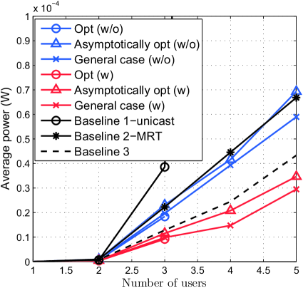
(a) Average power versus $K$. $M=4$, $\mathbf{r}=(2,2,3,3,4)$.

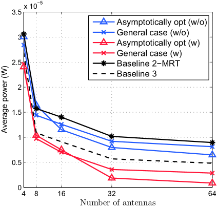
(b) Average power versus $M$. $K=4$, $\mathbf{r}=(2,3,3,4)$.

Figure 2: Average power versus $K$ and $M$.

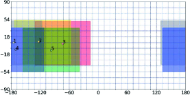
Figure 3: Viewing directions and corresponding FoVs of $5$ users [34].

First, we evaluate the average power over 1,000 random choices for the viewing directions of 1-5 users from 30 users from [34]. Fig. 2 (a) illustrates the average power versus the number of users $K$. Since the proposed optimal solutions for small multicast groups in the scenarios without and with user transcoding are valid only for $|\mathcal{K}_{\mathcal{S},l}|\leq 3,\mathcal{S}\in\mathcal{I},l\in\mathcal{L}_{\mathcal{S}}$, and $|\mathcal{S}|\leq 3,\mathcal{S}\in\mathcal{I}$, respectively. Therefore, we do not show their average powers for $K>3$ where the abovementioned conditions are not satisfied. We can observe that the average powers of the proposed solutions and baseline schemes increase with $K$, as the transmission load increases with $K$. When $K\leq 3$, the proposed solutions for the general case achieve close-to-optimal powers. Given the unsatisfactory performance of Baseline 1, we no longer compare with it in the remaining figures. Fig. 2 (b) illustrates the average power versus the number of antennas $M$. We can observe that the powers achieved by the proposed solutions and baseline schemes decrease with $M$. Also, when $M$ is sufficiently large, the proposed asymptotically optimal solutions reach close-to-optimal average powers, demonstrating the asymptotically optimalities of the proposed solutions for the case of a large antenna array.

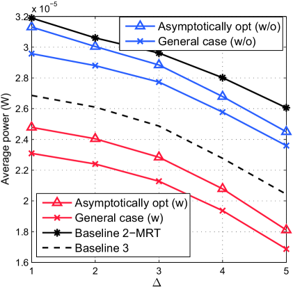
(a) Average power versus $\Delta$. $K=5$, $M=4$, $\mathbf{r}=(2,2,3,3,4)$.

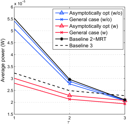
(b) Average power versus $\tau$. $K=5$, $M=4$.

Figure 4: Average power versus $\Delta$ and $\tau$.

Next, we show the impacts of the concentration of the viewing directions of all users and the similarity of the required quality levels of all users. We choose the viewing directions of 5 users out of 30 users from [34], i.e., $(\nu_{k},\gamma_{k})_{k\in\{1,\ldots,5\}}$, as shown in Fig. 3. To show the impact of the concentration of the viewing directions of all users, based on the chosen viewing directions, we consider five sets of viewing directions, i.e., $(\nu_{1}+\Delta,\gamma_{1}),(\nu_{2}+\Delta,\gamma_{2}),(\nu_{3},\gamma_{3}),(\nu_{4}-\Delta,\gamma_{4}),$ and $(\nu_{5}-\Delta,\gamma_{5})$, $\Delta=1,\ldots,5$, and evaluate the corresponding average powers. Note that $\Delta$ reflects the concentration of the viewing directions of the 5 users. In particular, the concentration increases with $\Delta$. Fig. 4 (a) shows the average power versus the concentration parameter $\Delta$. We can see that each multicast scheme’s average power decreases with $\Delta$, since multicast opportunities increase with $\Delta$. To show the impact of the similarity of the required quality levels, we consider three sets of required quality levels, i.e., $\bar{\mathbf{r}}_{\tau}=(\min\{\tau,3\},\min\{\tau+1,3\},3,\max\{3,5-\tau\},\max\{3,6-\tau\})$, $\tau=1,2,3$. Note that $\tau$ indicates the similarity of the required quality levels of the users. Specifically, the required quality levels are closer when $\tau$ is larger. Fig. 4 (b) illustrates the average power versus the similarity parameter $\tau$. We can see that when $\tau$ increases, the average power of each multicast scheme decreases, due to the rise of natural multicast opportunities. Furthermore, as $\tau$ increases, the gaps between the average powers of the multicast schemes in the scenario without user transcoding and those in the scenario with user transcoding decrease, as transcoding-enabled multicast opportunities decrease.

Fig. 2 and Fig. 4 show that the proposed solutions in the scenario with user transcoding outperform those in the scenario without user transcoding, which demonstrates the importance of using transcoding-enabled multicast opportunities in reducing power consumption. Fig. 2 and Fig. 4 also show that the proposed solutions outperform the baseline schemes. Specifically, the proposed solutions in the scenario without user transcoding outperform Baseline 1, as the proposed solutions utilizing multicast transmission offer higher spectral efficiency. The proposed solutions in the scenario without user transcoding outperform Baseline 2, as the proposed solutions carefully choose beamforming vectors. The proposed solutions in the scenario with user transcoding outperform Baseline 3, as the proposed solutions in the scenario with user transcoding optimally exploit transcoding-enabled multicast opportunities to reduce power consumption.

VI Conclusion

This paper studied the optimal wireless streaming of a multi-quality tiled 360 VR video to multiple users in a MIMO-OFDMA system. In the scenario without user transcoding, we minimized the total transmission power by optimizing the beamforming, and subcarrier, transmission power and rate allocation. This is a challenging mixed discrete-continuous optimization problem. We obtained a globally optimal solution for small multicast groups, an asymptotically optimal solution for a large antenna array, and a suboptimal solution for the general case. In the scenario with user transcoding, we minimized the weighted sum of the average total transmission power and the transcoding power by optimizing the quality level selection, beamforming, and subcarrier, transmission power, and rate allocation. This is a more challenging two-timescale mixed discrete-continuous optimization problem. We obtained a globally optimal solution for small multicast groups, an asymptotically optimal solution for a large antenna array, and a low-complexity suboptimal solution for the general case. Finally, numerical results showed that the proposed solutions have significant gains over existing schemes.

Appendix A: Proof of Theorem 1

First, we obtain a problem with the same optimal value as Problem 1. Let $(\bm{\mu}^{\star}(\mathbf{h}),\bm{\eta}^{\star}(\mathbf{h}),\mathbf{c}^{\star}(\mathbf{h})$, $\mathbf{w}^{\star}(\mathbf{h}))$ denote an optimal solution of Problem 1. By contradiction, we can easily show

$$c^{\star}_{\mathcal{S},l,n}(\mathbf{h})= \mu^{\star}_{\mathcal{S},l,n}(\mathbf{h})B\log_{2}\left(1+\right.$$

$$\left.\frac{\eta^{\star}_{\mathcal{S},l,n}(\mathbf{h})\min\limits_{k\in\mathcal{K}_{\mathcal{S},l}}\beta_{k}|\mathbf{h}_{k,n}^{H}\mathbf{w}^{\star}_{n}(\mathbf{h})|^{2}}{M\sigma^{2}}\right).$$

Thus, equivalently, we can eliminate $\mathbf{c}(\mathbf{h})$ and replace the constraints in (5), (6), and (7) with

$$\sum\limits_{n\in\mathcal{N}}\mu_{\mathcal{S},l,n}(\mathbf{h})B\log_{2}\left(1+\frac{\eta_{\mathcal{S},l,n}(\mathbf{h})\min\limits_{k\in\mathcal{K}_{\mathcal{S},l}}\beta_{k}|\mathbf{h}_{k,n}^{H}\mathbf{w}_{n}(\mathbf{h})|^{2}}{M\sigma^{2}}\right)$$

$$\geq|\mathcal{P}_{\mathcal{S}}|D_{l},~{}\mathcal{S}\in\mathcal{I},l\in\mathcal{L}_{\mathcal{S}}.$$ (51)

Define $P_{\mathcal{S},l,n}(\mathbf{h})=\mu_{\mathcal{S},l,n}(\mathbf{h})\eta_{\mathcal{S},l,n}(\mathbf{h})$, $\mathbf{\tilde{w}}_{\mathcal{S},l,n}(\mathbf{h})=\mathbf{w}_{n}(\mathbf{h})$, and

$$\widetilde{Q}_{\mathcal{S},l,n}(\mathbf{h})=\max\limits_{k\in\mathcal{K}_{\mathcal{S},l}}\frac{M\sigma^{2}}{\beta_{k}|\mathbf{h}_{k,n}^{H}\mathbf{w}_{n}(\mathbf{h})|^{2}},\mathcal{S}\in\mathcal{I},l\in\mathcal{L}_{\mathcal{S}},n\in\mathcal{N}.$$ (52)

By the change of variables of $\mathbf{P}(\mathbf{h})\triangleq(P_{\mathcal{S},l,n}(\mathbf{h}))_{\mathcal{S}\in\mathcal{I},l\in\mathcal{L}_{\mathcal{S}},n\in\mathcal{N}}$ and $\mathbf{\tilde{w}}(\mathbf{h})\triangleq(\tilde{\mathbf{w}}_{\mathcal{S},l,n}(\mathbf{h}))_{\mathcal{S}\in\mathcal{I},l\in\mathcal{L}_{\mathcal{S}},n\in\mathcal{N}}$, and introducing the auxiliary variable $\mathbf{\widetilde{Q}}(\mathbf{h})\triangleq(\widetilde{Q}_{\mathcal{S},l,n}(\mathbf{h}))_{\mathcal{S}\in\mathcal{I},l\in\mathcal{L}_{\mathcal{S}},n\in\mathcal{N}}$, the constraints in (4) and (51) can be transformed to (52) and the following constraints:

$$\|\tilde{\mathbf{w}}_{\mathcal{S},l,n}(\mathbf{h})\|_{2}=1,~{}\mathcal{S}\in\mathcal{I},l\in\mathcal{L}_{\mathcal{S}},n\in\mathcal{N},$$ (53)

$$\tilde{\mathbf{w}}_{\mathcal{S},l,n}(\mathbf{h})=\tilde{\mathbf{w}}_{\mathcal{S}^{\prime},l^{\prime},n}(\mathbf{h}),~{}\mathcal{S},\mathcal{S}^{\prime}\in\mathcal{I},l\in\mathcal{L}_{\mathcal{S}},l^{\prime}\in\mathcal{L}_{\mathcal{S}^{\prime}},n\in\mathcal{N},$$ (54)

$$\sum\limits_{n\in\mathcal{N}}\mu_{\mathcal{S},l,n}(\mathbf{h})B\log_{2}\left(1+\frac{P_{\mathcal{S},l,n}(\mathbf{h})}{\mu_{\mathcal{S},l,n}(\mathbf{h})\widetilde{Q}_{\mathcal{S},l,n}(\mathbf{h})}\right)$$

$$\geq|\mathcal{P}_{\mathcal{S}}|D_{l},~{}\mathcal{S}\in\mathcal{I},l\in\mathcal{L}_{\mathcal{S}}.$$ (55)

In addition, by contradiction, we can easily show that (52) can be equivalently replaced by the following constraints:

$$\begin{matrix}\widetilde{Q}_{\mathcal{S},l,n}(\mathbf{h})\geq\max\limits_{k\in\mathcal{K}_{\mathcal{S},l}}\frac{M\sigma^{2}}{\beta_{k}|\mathbf{h}_{k,n}^{H}\mathbf{\tilde{w}}_{\mathcal{S},l,n}(\mathbf{h})|^{2}},~{}\mathcal{S}\in\mathcal{I},l\in\mathcal{L}_{\mathcal{S}},n\in\mathcal{N}.\end{matrix}$$ (56)

Thus, Problem 1 and the following problem have the same optimal value.

Problem 13 (Equivalent Problem of Problem 1)

$$E^{\star}(\mathbf{h})=\min_{\bm{\mu}(\mathbf{h}),\mathbf{P}(\mathbf{h}),\mathbf{\tilde{w}}(\mathbf{h}),\mathbf{\widetilde{Q}}(\mathbf{h})}~{} \frac{1}{M}\sum\limits_{n\in\mathcal{N}}\sum\limits_{\mathcal{S}\in\mathcal{I}}\sum\limits_{l\in\mathcal{L}_{\mathcal{S}}}P_{\mathcal{S},l,n}(\mathbf{h})$$

$$\mathrm{s.t.}~{}~{}\eqref{cst:mu1},~{}\eqref{cst:mu2}, ~{}\eqref{cst:p},~{}\eqref{pf-tw},~{}\eqref{pf-tw2},~{}\eqref{pfcst-w0},~{}\eqref{cst:Q2}.$$

Denote $(\bm{\mu}^{\star}(\mathbf{h}),\bm{P}^{\star}(\mathbf{h}),\mathbf{\tilde{w}}^{\star}(\mathbf{h}),\widetilde{\mathbf{Q}}^{\star}(\mathbf{h}))$ an optimal solution.

Then, we obtain a problem with the same optimal value as Problem 13. Consider the following problem.

Problem 14 (Equivalent Problem of Problem 13)

$$E^{\ddagger}(\mathbf{h})=\min_{\bm{\mu}(\mathbf{h}),\mathbf{P}(\mathbf{h}),\mathbf{\tilde{w}}(\mathbf{h}),\mathbf{\widetilde{Q}}(\mathbf{h})}~{} \frac{1}{M}\sum\limits_{n\in\mathcal{N}}\sum\limits_{\mathcal{S}\in\mathcal{I}}\sum\limits_{l\in\mathcal{L}_{\mathcal{S}}}P_{\mathcal{S},l,n}(\mathbf{h})$$

$$\mathrm{s.t.}~{}~{}\eqref{cst:mu1},~{} \eqref{cst:mu2},~{}\eqref{cst:p},~{}\eqref{pf-tw},~{}\eqref{pfcst-w0},~{}\eqref{cst:Q2}.$$

Let $(\bm{\mu}^{\ddagger}(\mathbf{h}),\bm{P}^{\ddagger}(\mathbf{h}),\mathbf{\tilde{w}}^{\ddagger}(\mathbf{h}),\widetilde{\mathbf{Q}}^{\ddagger}(\mathbf{h}))$ denote an optimal solution. As Problem 13 has extra constraints, i.e., (54), compared to Problem 14, $E^{\star}(\mathbf{h})\geq E^{\ddagger}(\mathbf{h})$. Thus, it remains to show that $E^{\star}(\mathbf{h})\leq E^{\ddagger}(\mathbf{h})$. Based on an optimal solution of Problem 14, i.e., $(\bm{\mu}^{\ddagger}(\mathbf{h}),\bm{P}^{\ddagger}(\mathbf{h}),\mathbf{\tilde{w}}^{\ddagger}(\mathbf{h}),\widetilde{\mathbf{Q}}^{\ddagger}(\mathbf{h}))$, we construct a feasible solution of Problem 13, whose objective value is $E^{\ddagger}(\mathbf{h})$. Specifically, for all $n\in\mathcal{N}$, we construct $\mathbf{\tilde{w}}^{\diamond}_{\mathcal{S},l,n}(\mathbf{h})=\mathbf{\tilde{w}}^{\ddagger}_{\mathcal{S}_{n},l_{n},n}(\mathbf{h})$, $\mathcal{S}\in\mathcal{I}$, $l\in\mathcal{L}_{\mathcal{S}}$, where $(\mathcal{S}_{n},l_{n})$ satisfies $\mu_{\mathcal{S},l,n}^{\ddagger}(\mathbf{h})=1$. It is obvious that $(\bm{\mu}^{\ddagger}(\mathbf{h}),\bm{P}^{\ddagger}(\mathbf{h}),\mathbf{\tilde{w}}^{\diamond}(\mathbf{h}),\widetilde{\mathbf{Q}}^{\ddagger}(\mathbf{h}))$ is a feasible solution of Problem 13. Thus, we have $E^{\star}(\mathbf{h})\leq\frac{1}{M}\sum\nolimits_{n\in\mathcal{N}}\sum\nolimits_{\mathcal{S}\in\mathcal{I}}\sum\nolimits_{l\in\mathcal{L}_{\mathcal{S}}}P^{\ddagger}_{\mathcal{S},l,n}(\mathbf{h})=E^{\ddagger}(\mathbf{h}).$ By $E^{\star}(\mathbf{h})\geq E^{\ddagger}(\mathbf{h})$ and $E^{\star}(\mathbf{h})\leq E^{\ddagger}(\mathbf{h})$, we have $E^{\star}(\mathbf{h})=E^{\ddagger}(\mathbf{h})$.

Next, we show that Problem 14 and Problem 2 have the same optimal value. It is obvious that Problem 14 is equivalent to the following problem.

Problem 15 (Equivalent Problem of Problem 14 for $\mathbf{h}$)

$$E^{\ddagger}(\mathbf{h})=\min_{\bm{\mu}(\mathbf{h}),\mathbf{P}(\mathbf{h})}~{}\frac{1}{M}\sum\limits_{n\in\mathcal{N}}\sum\limits_{\mathcal{S}\in\mathcal{I}}\sum\limits_{l\in\mathcal{L}_{\mathcal{S}}}P_{\mathcal{S},l,n}(\mathbf{h})$$

$$\mathrm{s.t.}~{}~{}\eqref{cst:mu1},~{}\eqref{cst:mu2},~{}\eqref{cst:p},$$

$$\sum\nolimits_{n\in\mathcal{N}}\mu_{\mathcal{S},l,n}(\mathbf{h})B\log_{2}\left(1+\frac{P_{\mathcal{S},l,n}(\mathbf{h})}{\mu_{\mathcal{S},l,n}(\mathbf{h})\widetilde{Q}_{\mathcal{S},l,n}^{\star}(\mathbf{h})}\right)$$

$$\geq|\mathcal{P}_{\mathcal{S}}|D_{l},~{}\mathcal{S}\in\mathcal{I},l\in\mathcal{L}_{\mathcal{S}},k\in\mathcal{K}_{\mathcal{S},l},$$ (57)

where $\widetilde{Q}_{\mathcal{S},l,n}^{\star}(\mathbf{h})$ is given by the following problem.

$$\widetilde{Q}_{\mathcal{S},l,n}^{\star}(\mathbf{h})\triangleq \min_{\tilde{\mathbf{w}}_{\mathcal{S},l,n}(\mathbf{h})}\max_{k\in\mathcal{K}_{\mathcal{S},l}}\frac{M\sigma^{2}}{\beta_{k}|\mathbf{h}_{k,n}^{H}\tilde{\mathbf{w}}_{\mathcal{S},l,n}(\mathbf{h})|^{2}}$$ (58)

$$\mathrm{s.t.}~{}~{}\eqref{pf-tw}.$$

As

$$Q^{\dagger}_{\mathcal{S},l,n}(\mathbf{h})\overset{(a)}{=}\frac{\text{tr}(\mathbf{V}_{\mathcal{S},l,n}^{\dagger}(\mathbf{h}))}{\|\tilde{\mathbf{w}}_{\mathcal{S},l,n}^{\star}(\mathbf{h})\|_{2}^{2}}$$

$$\overset{(b)}{=}\left(\min_{k\in\mathcal{K}_{\mathcal{S},l}}\frac{\text{tr}(\beta_{k}\mathbf{h}_{k,n}\mathbf{h}_{k,n}^{H}\mathbf{V}^{\dagger}_{\mathcal{S},l,n})}{M\sigma^{2}}\right)\left(\max_{k\in\mathcal{K}_{\mathcal{S},l}}\frac{M\sigma^{2}}{\beta_{k}|\mathbf{h}_{k,n}^{H}\tilde{\mathbf{w}}_{\mathcal{S},l,n}^{\star}(\mathbf{h})|^{2}}\right)$$

$$\overset{(c)}{=}\max_{k\in\mathcal{K}_{\mathcal{S},l}}\frac{M\sigma^{2}}{\beta_{k}|\mathbf{h}_{k,n}^{H}\tilde{\mathbf{w}}_{\mathcal{S},l,n}^{\star}(\mathbf{h})|^{2}}=\tilde{Q}^{\star}_{\mathcal{S},l,n}(\mathbf{h}),$$ (59)

where $(a)$ is due to (53), $(b)$ is due to Claim 2 in [23], and $(c)$ is due to that $\frac{\min_{k\in\mathcal{K}_{\mathcal{S},l}}\text{tr}(\beta_{k}\mathbf{h}_{k,n}\mathbf{h}_{k,n}^{H}\mathbf{V}^{\dagger}_{\mathcal{S},l,n})}{M\sigma^{2}}=1$ (which can be easily shown by contradiction), $E^{\ddagger}(\mathbf{h})=E^{\dagger}(\mathbf{h})$.

Finally, we show that Problem 1 and Problem 2 have the same optimal value and characterize the relation between their optimal solutions. As $E^{\star}(\mathbf{h})=E^{\ddagger}(\mathbf{h})$ and $E^{\ddagger}(\mathbf{h})=E^{\dagger}(\mathbf{h})$, we know that the optimal values of Problem 1 and Problem 2 are identical, i.e.,

$$E^{\star}(\mathbf{h})=E^{\dagger}(\mathbf{h}).$$ (60)

In the sequel, we show that $(\bm{\mu}^{\dagger}(\mathbf{h}),\bm{\eta}^{\dagger}(\mathbf{h}),\mathbf{c}^{\dagger}(\mathbf{h}),\mathbf{w}^{\dagger}(\mathbf{h}))$ is an optimal solution of Problem 1. It is obvious that $(\bm{\mu}^{\dagger}(\mathbf{h}),\bm{\eta}^{\dagger}(\mathbf{h}),\mathbf{c}^{\dagger}(\mathbf{h}),\mathbf{w}^{\dagger}(\mathbf{h}))$ satisfies the constraints in (1), (2), (3), (5), and (7). It remains to show that $(\bm{\mu}^{\dagger}(\mathbf{h}),\bm{\eta}^{\dagger}(\mathbf{h}),\mathbf{c}^{\dagger}(\mathbf{h}),\mathbf{w}^{\dagger}(\mathbf{h}))$ satisfies (4) and (6). We have

$$\|\mathbf{v}_{\mathcal{S},l,n}^{\dagger}(\mathbf{h})\|_{2}\overset{(d)}{=}\sqrt{\text{tr}\left(\mathbf{V}_{\mathcal{S},l,n}^{\dagger}(\mathbf{h})\right)}=\sqrt{Q^{\dagger}_{\mathcal{S},l,n}(\mathbf{h})},$$ (61)

where $(d)$ is due to $\mathbf{V}_{\mathcal{S},l,n}^{\dagger}(\mathbf{h})=\mathbf{v}_{\mathcal{S},l,n}^{\dagger}(\mathbf{h})(\mathbf{v}_{\mathcal{S},l,n}^{\dagger}(\mathbf{h}))^{H}$. Thus, we have

$$\|\mathbf{w}^{\dagger}_{n}(\mathbf{h})\|_{2}\overset{(e)}{=}\|\sum\limits_{\mathcal{S}\in\mathcal{I}}\sum\limits_{l\in\mathcal{L}_{\mathcal{S}}}\mu_{\mathcal{S},l,n}^{\dagger}(\mathbf{h})\frac{\mathbf{v}^{\dagger}_{\mathcal{S},l,n}(\mathbf{h})}{\|\mathbf{v}_{\mathcal{S},l,n}^{\dagger}(\mathbf{h})\|_{2}}\|_{2}\overset{(f)}{=}1,$$ (62)

where $(e)$ is due to (13) and (61), and $(f)$ is due to (1) and (2). Thus, $\mathbf{w}^{\dagger}(\mathbf{h})$ satisfies (4). Besides, we have

$$\mu_{\mathcal{S},l,n}^{\dagger}(\mathbf{h})B\log_{2}\left(1+\frac{\eta_{\mathcal{S},l,n}^{\dagger}(\mathbf{h})\beta_{k}|\mathbf{h}_{n,k}^{H}\mathbf{w}_{n}(\mathbf{h})|^{2}}{M\sigma^{2}}\right)$$

$$\overset{(g)}{\geq}\mu_{\mathcal{S},l,n}^{\dagger}(\mathbf{h})B\log_{2}\left(1+\frac{P_{\mathcal{S},l,n}^{\dagger}(\mathbf{h})\beta_{k}|\mathbf{h}_{n,k}^{H}\mathbf{v}^{\dagger}_{\mathcal{S},l,n}(\mathbf{h})|^{2}}{M\sigma^{2}Q_{\mathcal{S},l,n}^{\dagger}(\mathbf{h})}\right)$$

$$\overset{(h)}{\geq}\mu_{\mathcal{S},l,n}^{\dagger}(\mathbf{h})B\log_{2}\left(1+\frac{P_{\mathcal{S},l,n}^{\dagger}(\mathbf{h})}{Q_{\mathcal{S},l,n}^{\dagger}(\mathbf{h})}\right)=c_{\mathcal{S},l,n}^{\dagger}(\mathbf{h}),$$ (63)

where $(g)$ is due to (12), (13), (1) and (2), and $(h)$ is due to (10) and $\mathbf{V}_{\mathcal{S},l,n}^{\dagger}(\mathbf{h})=\mathbf{v}_{\mathcal{S},l,n}^{\dagger}(\mathbf{h})(\mathbf{v}_{\mathcal{S},l,n}^{\dagger}(\mathbf{h}))^{H}$. Thus, $(\bm{\mu}^{\dagger}(\mathbf{h}),\bm{\eta}^{\dagger}(\mathbf{h}),\mathbf{c}^{\dagger}(\mathbf{h}),\mathbf{w}^{\dagger}(\mathbf{h}))$ satisfies (6). Therefore, $(\bm{\mu}^{\dagger}(\mathbf{h}),\bm{\eta}^{\dagger}(\mathbf{h}),\mathbf{c}^{\dagger}(\mathbf{h}),\mathbf{w}^{\dagger}(\mathbf{h}))$ is a feasible solution of Problem 1, implying

$$E^{\star}(\mathbf{h}) \leq\sum\nolimits_{n\in\mathcal{N}}\sum\nolimits_{\mathcal{S}\in\mathcal{I}}\sum\nolimits_{l\in\mathcal{L}_{\mathcal{S}}}\frac{\mu^{\dagger}_{\mathcal{S},l,n}(\mathbf{h})\eta^{\dagger}_{\mathcal{S},l,n}(\mathbf{h})}{M}$$

$$\overset{(i)}{\leq}\sum\limits_{n\in\mathcal{N}}\sum\limits_{\mathcal{S}\in\mathcal{I}}\sum\limits_{l\in\mathcal{L}_{\mathcal{S}}}\frac{P_{\mathcal{S},l,n}^{\dagger}(\mathbf{h})}{M}=E^{\dagger}(\mathbf{h})\overset{(j)}{=}E^{\star}(\mathbf{h}),$$ (64)

where $(i)$ is due to (1), (2) and (12), and $(j)$ is due to (60). Thus, we can conclude that $(\bm{\mu}^{\dagger}(\mathbf{h}),\bm{\eta}^{\dagger}(\mathbf{h}),\mathbf{c}^{\dagger}(\mathbf{h}),\mathbf{w}^{\dagger}(\mathbf{h}))$ achieves the optimal value of Problem 1 and is an optimal solution of Problem 1.

Appendix B: Proof of Theorem 2

First, we show that the problem in (58) and Problem 3 are equivalent. We have

$$\tilde{\mathbf{w}}_{\mathcal{S},l,n}^{\star}(\mathbf{h})\overset{(a)}{=} \frac{\tilde{\mathbf{w}}_{\mathcal{S},l,n}^{\star}(\mathbf{h})}{\|\tilde{\mathbf{w}}_{\mathcal{S},l,n}^{\star}(\mathbf{h})\|}\overset{(b)}{=}\frac{\mathbf{v}_{\mathcal{S},l,n}^{\dagger}(\mathbf{h})}{\|\mathbf{v}_{\mathcal{S},l,n}^{\dagger}(\mathbf{h})\|}\overset{(c)}{=}\frac{\mathbf{v}_{\mathcal{S},l,n}^{\dagger}(\mathbf{h})}{\sqrt{Q^{\dagger}_{\mathcal{S},l,n}(\mathbf{h})}}$$

$$\overset{(d)}{=} \frac{\mathbf{v}_{\mathcal{S},l,n}^{\dagger}(\mathbf{h})}{\sqrt{\max_{k\in\mathcal{K}_{\mathcal{S},l}}\frac{M\sigma^{2}}{\beta_{k}|\mathbf{h}_{k,n}^{H}\tilde{\mathbf{w}}_{\mathcal{S},l,n}^{\star}(\mathbf{h})|^{2}}}},$$ (65)

where $(a)$ is due to (53), $(b)$ is due to Claim 2 in [23], $(c)$ is due to (61), and $(d)$ is due to (59). Thus, we have

$$\mathbf{V}_{\mathcal{S},l,n}^{\dagger}(\mathbf{h})=\mathbf{v}_{\mathcal{S},l,n}^{\dagger}(\mathbf{h})(\mathbf{v}_{\mathcal{S},l,n}^{\dagger}(\mathbf{h}))^{H}$$

$$=\tilde{\mathbf{w}}_{\mathcal{S},l,n}^{\star}(\mathbf{h})(\tilde{\mathbf{w}}_{\mathcal{S},l,n}^{\star}(\mathbf{h}))^{H}\max_{k\in\mathcal{K}_{\mathcal{S},l}}\frac{M\sigma^{2}}{\beta_{k}|\mathbf{h}_{k,n}^{H}\tilde{\mathbf{w}}_{\mathcal{S},l,n}^{\star}(\mathbf{h})|^{2}}.$$ (66)

By (59) and (66), we can conclude that the problem in (58) and Problem 3 are equivalent.

Next, we obtain an asymptotically optimal solution of the problem in (58). Following the proof of Theorem 1 in [29], we can show that $\mathbf{\tilde{w}}_{\mathcal{S},l,n}^{\ast}(\mathbf{h})=\frac{\sum\nolimits_{k\in\mathcal{K}_{\mathcal{S},l}}\xi_{n,k}^{\ast}\mathbf{h}_{n,k}}{\left\|\sum\nolimits_{k\in\mathcal{K}_{\mathcal{S},l}}\xi_{n,k}^{\ast}\mathbf{h}_{n,k}\right\|_{2}}$ is asymptotically optimal for the problem in (58), where $\xi_{n,k}^{\ast}$ is an optimal solution of the following problem:

$$\min_{\xi_{n,k}}\max_{k\in\mathcal{K}_{\mathcal{S},l}}\frac{\sigma^{2}\sum\nolimits_{j\in\mathcal{K}}\xi_{n,j}^{2}}{\beta_{k}\xi_{n,k}^{2}}.$$ (67)

This problem is similar to Problem $\mathcal{Q}$ in [29]. Using the method proposed in [29], we have $\xi^{\ast}_{n,k}=\frac{1}{\sqrt{\beta_{k}}}$. Thus, the asymptotically optimal solution of the problem in (58) can be written as $\mathbf{\tilde{w}}_{\mathcal{S},l,n}^{\ast}(\mathbf{h})=\frac{\sum\nolimits_{k\in\mathcal{K}_{\mathcal{S},l}}\frac{1}{\sqrt{\beta_{k}}}\mathbf{h}_{n,k}}{\left\|\sum\nolimits_{k\in\mathcal{K}_{\mathcal{S},l}}\frac{1}{\sqrt{\beta_{k}}}\mathbf{h}_{n,k}\right\|_{2}}$.

Finally, we show that $\mathbf{V}_{\mathcal{S},l,n}^{\ast}(\mathbf{h})$ is an asymptotically optimal solution of Problem 3. By $\mathbf{V}_{\mathcal{S},l,n}^{\ast}(\mathbf{h})=\mathbf{v}_{\mathcal{S},l,n}^{\ast}(\mathbf{h})(\mathbf{v}_{\mathcal{S},l,n}^{\ast}(\mathbf{h}))^{H}$ and (22), we have

$$\mathbf{V}_{\mathcal{S},l,n}^{\ast}(\mathbf{h})=\tilde{\mathbf{w}}_{\mathcal{S},l,n}^{\ast}(\mathbf{h})(\tilde{\mathbf{w}}_{\mathcal{S},l,n}^{\ast}(\mathbf{h}))^{H}\max_{k\in\mathcal{K}_{\mathcal{S},l}}\frac{M\sigma^{2}}{\beta_{k}|\mathbf{h}_{k,n}^{H}\tilde{\mathbf{w}}_{\mathcal{S},l,n}^{\ast}(\mathbf{h})|^{2}}.$$ (68)

Since $\tilde{\mathbf{w}}_{\mathcal{S},l,n}^{\ast}(\mathbf{h})$ is an asymptotically optimal solution of the problem in (58) , by (66) and (68), we can conclude that $\mathbf{V}_{\mathcal{S},l,n}^{\ast}(\mathbf{h})$ is an asymptotically optimal solution of Problem 3.

Appendix C: Proof of Theorem 3

First, we show that the optimal value of Problem 10 is no greater than that of Problem 11, i.e., $E_{t}^{\dagger}\leq\bar{E}_{t}^{\ast}$. Based on an optimal solution of Problem 11, i.e., $(\bar{\mathbf{N}}^{\ast},\bar{\mathbf{P}}^{\ast},\mathbf{x}^{\ast})$, we construct a feasible solution of Problem 10, whose objective value is $\bar{E}^{\ast}$. Specifically, we construct $\bar{\mu}^{\ast}_{\mathcal{S},l,n}=\frac{\bar{N}^{\ast}_{\mathcal{S},l}}{N}$, $\bar{p}^{\ast}_{\mathcal{S},l,n}=\frac{\bar{P}^{\ast}_{\mathcal{S},l}}{N}$, $\mathcal{S}\in\mathcal{I},l\in\mathcal{L},n\in\mathcal{N}$. Then, it is obvious that $(\bm{\bar{\mu}}^{\ast},\bm{\bar{p}}^{\ast},\mathbf{x}^{\ast})$ satisfies the constraints of Problem 10, implying that it is a feasible solution of Problem 10. Besides, we have

$$E_{t}^{\dagger}\leq\sum\limits_{n\in\mathcal{N}}\sum\limits_{\mathcal{S}\in\mathcal{I}}\sum\limits_{l\in\mathcal{L}}\frac{\bar{p}^{\ast}_{\mathcal{S},l,n}}{M}+\alpha E_{\text{tc}}(\mathbf{x}^{\ast})\overset{(a)}{=}\bar{E}_{t}^{\ast},$$ (69)

where $(a)$ is due to $\bar{\mu}^{\ast}_{\mathcal{S},l,n}=\frac{\bar{N}^{\ast}_{\mathcal{S},l}}{N}$, $\bar{p}^{\ast}_{\mathcal{S},l,n}=\frac{\bar{P}^{\ast}_{\mathcal{S},l}}{N}$.

Next, we show that the optimal value of Problem 10 is no smaller than that of Problem 11, i.e., $E_{t}^{\dagger}\geq\bar{E}_{t}^{\ast}$. Base on an optimal solution of Problem 10, i.e., $(\bar{\bm{\mu}}^{\dagger},\bar{\bm{p}}^{\dagger},\mathbf{x}^{\dagger})$, we construct a feasible solution of Problem 11, whose objective value is $E_{t}^{\dagger}$. Specifically, we construct $\bar{N}^{\dagger}_{\mathcal{S},l}=\sum\nolimits_{n\in\mathcal{N}}\bar{\mu}^{\dagger}_{\mathcal{S},l,n}$, $\bar{P}^{\dagger}_{\mathcal{S},l}=\sum\nolimits_{n\in\mathcal{N}}\bar{p}^{\dagger}_{\mathcal{S},l,n}$, $\mathcal{S}\in\mathcal{I},l\in\mathcal{L},n\in\mathcal{N}$. It is obvious that $(\bm{\bar{N}}^{\dagger},\bm{\bar{P}}^{\dagger},\mathbf{x}^{\dagger})$ satisfies the constraints in (31), (32), (33), (44), (45), and (46). We also have

$$\frac{1}{N}\bar{N}^{\dagger}_{\mathcal{S},l}B\log_{2}\left(1+\frac{\bar{P}^{\dagger}_{\mathcal{S},l}}{\bar{Q}_{k}\bar{N}^{\dagger}_{\mathcal{S},l}}\right)$$

$$=\left(\sum\limits_{n\in\mathcal{N}}\frac{1}{N}\bar{\mu}^{\dagger}_{\mathcal{S},l,n}\right)B\log_{2}\left(1+\frac{\sum\limits_{n\in\mathcal{N}}\frac{1}{N}\bar{p}^{\dagger}_{\mathcal{S},l,n}}{\bar{Q}_{k}\sum\limits_{n\in\mathcal{N}}\frac{1}{N}\bar{\mu}_{\mathcal{S},l,n}}\right)$$

$$\overset{(b)}{\geq}\sum\limits_{n\in\mathcal{N}}\bar{\mu}^{\dagger}_{\mathcal{S},l,n}B\log_{2}\left(1+\frac{\bar{p}^{\dagger}_{\mathcal{S},l,n}}{\bar{Q}_{k}\bar{\mu}^{\dagger}_{\mathcal{S},l,n}}\right)$$

$$\overset{(c)}{\geq}|\mathcal{P}_{\mathcal{S}}|D_{l}x_{\mathcal{S},l,k},~{}\mathcal{S}\in\mathcal{I},l\in\mathcal{L},k\in\mathcal{S},n\in\mathcal{N},$$ (70)

where $(b)$ is due to the concavity of $\bar{\mu}_{\mathcal{S},l,n}B\log_{2}\left(1+\frac{\bar{p}_{\mathcal{S},l,n}}{\bar{Q}_{k}\bar{\mu}_{\mathcal{S},l,n}}\right)$ in $(\bar{\mu}_{\mathcal{S},l,n},\bar{p}_{\mathcal{S},l,n})$, and $(c)$ is due to (40). By (70), we know that $(\bm{\bar{N}}^{\dagger},\bm{\bar{P}}^{\dagger},\mathbf{x}^{\dagger})$ satisfies the constraints in (47). Thus, $(\bm{\bar{N}}^{\dagger},\bm{\bar{P}}^{\dagger},\mathbf{x}^{\dagger})$ is a feasible solution of Problem 11. In addition, we have

$$E_{t}^{\dagger}\overset{(d)}{=}\frac{1}{M}\sum\nolimits_{\mathcal{S}\in\mathcal{I}}\sum\nolimits_{l\in\mathcal{L}}\bar{P}^{\dagger}_{\mathcal{S},l}+\alpha E_{\text{tc}}(\mathbf{x}^{\dagger})\geq\bar{E}_{t}^{\ast},$$ (71)

where $(d)$ is due to $\bar{N}^{\dagger}_{\mathcal{S},l}=\sum\nolimits_{n\in\mathcal{N}}\bar{\mu}^{\dagger}_{\mathcal{S},l,n}$, $\bar{P}^{\dagger}_{\mathcal{S},l}=\sum\nolimits_{n\in\mathcal{N}}\bar{p}^{\dagger}_{\mathcal{S},l,n}$, $\mathcal{S}\in\mathcal{I},l\in\mathcal{L},n\in\mathcal{N}$.

Finally, we show that the optimal values of Problem 10 and Problem 11 are identical and characterize the relatioship between their optimal solutions. By (69) and (71), we have $E_{t}^{\dagger}=\bar{E}_{t}^{\ast}$. By $E_{t}^{\dagger}=\bar{E}_{t}^{\ast}$ and (69), we know that $(\bm{\bar{\mu}}^{\ast},\bm{\bar{p}}^{\ast},\mathbf{x}^{\ast})$ is an optimal solution of Problem 10. By $E_{t}^{\dagger}=\bar{E}_{t}^{\ast}$ and (71), we know that $(\bm{\bar{N}}^{\dagger},\bm{\bar{P}}^{\dagger},\mathbf{x}^{\dagger})$ is an optimal solution of Problem 11. Therefore, the proof of Theorem 3 is completed.

References

[1]
C. Guo, Y. Cui, Z. Liu, and D. Ng, “Optimal transmission of multi-quality tiled 360 VR video in MIMO-OFDMA systems,”
in Proc. of IEEE ICC, Jun. 2021.
[2]
R. Ju, J. He, F. Sun, J. Li, F. Li, J. Zhu, and L. Han, “Ultra wide view based
panoramic VR streaming,” in Proc. of the Workshop on
VR/AR Network, Aug. 2017, pp. 19–23.
[4]
T. Dang, and M. Peng, “Joint radio communication, caching, and computing design for mobile virtual reality delivery in fog radio access networks,” IEEE J. Select. Areas Commun., vol. 37, no. 7, pp. 1594-1607, Jul. 2019.
[5]
M. Chen, W. Saad, and C. Yin, “Virtual reality over wireless networks: quality-of-service model and learning-based resource management,” IEEE Trans. Commun., vol. 66, no. 11, pp. 5621-5635, Nov. 2018.
[6]
Y. Sun, Z. Chen, M. Tao, and H. Liu, “Communications, caching, and computing for mobile virtual reality: modeling and tradeoff,” IEEE Trans. Commun., vol. 67, no. 11, pp. 7573-7586, Nov. 2019.
[7]
V. R. Gaddam, M. Riegler, R. Eg, C. Griwodz, and P. Halvorsen, “Tiling in
interactive panoramic video: approaches and evaluation,” IEEE Trans.
Multimedia, vol. 18, no. 9, pp. 1819–1831, Sep. 2016.
[8]
X. Lan, X. Zhang, and Z. Guo, “CLS: A cross-user learning based system for improving QoE in 360-degree video adaptive streaming,” in Proc. of ACM Multimedia, Oct. 2018, pp. 564-572.
[9]
C. Jacob, R. Aksu, X. Corbillon, G. Simon, and V. Swaminathan, “Viewport-driven rate-distortion optimized 360 video streaming,” in Proc. of IEEE ICC, May 2018, pp. 1-7.
[10]
D. V. Nguyen, H. T. T. Tran, A. T. Pham, and T. C. Thang, “An optimal tile-based approach for viewport-adaptive 360-degree video streaming,” IEEE J. Emerging and Select. Top. Circuits Syst., vol. 9, no. 1, pp. 29-42, Mar. 2019.
[11]
C. Perfecto, M. S. Elbamby, J. D. Ser, and M. Bennis, “Taming the latency in multi-user VR 360: a QoE-aware deep learning-aided multicast framework,” IEEE Trans. on Commun, vol. 68, no. 4, pp. 2491-2508, Apr. 2020.
[12]
F. Hu, Y. Deng, and A. H. Aghvami, “Correlation-aware cooperative multigroup broadcast 360 video delivery network: a hierarchical deep reinforcement learning approach,” arXiv preprint arXiv:2010.11347, Oct. 2020.
[13]
C. Guo, Y. Cui, and Z. Liu, “Optimal multicast of tiled 360 VR
video,” IEEE Wireless Commun. Lett., vol. 8, no. 1, pp. 145–148,
Feb. 2019.
[14]
——, “Optimal multicast of tiled 360 VR video in OFDMA
systems,” IEEE Commun. Lett., vol. 22, no. 12, pp. 2563–2566, Oct.
2018.
[15]
H. Ahmadi, O. Eltobgy, and M. Hefeeda, “Adaptive multicast streaming of
virtual reality content to mobile users,” in Proc. of the on Thematic
Workshops of ACM Multimedia, Oct. 2017, pp. 170–178.
[16]
Z. Zhilong, Z. Ma, Y. Sun, and D. Liu, “Wireless multicast of virtual
reality videos with MPEG-I format,” IEEE Access, vol. 7,
pp. 176 693–176 705, Dec. 2019.
[17]
N. Kan, C. Liu, J. Zou, C. Li, and H. Xiong, “A server-side
optimized hybrid multicast-unicast strategy for multi-user adaptive
360-degree video streaming,” in Proc. of IEEE ICIP, Sep. 2019, pp.
141–145.
[18]
K. Long, C. Ye, Y. Cui, and Z. Liu, “Optimal multi-quality multicast for 360
virtual reality video,” in Proc. of IEEE GLOBECOM, Dec. 2018, pp.
1–6.
[19]
K. Long, Y. Cui, C. Ye, and Z. Liu, “Optimal wireless streaming of multi-quality 360 VR video by exploiting natural, relative smoothness-enabled and transcoding-enabled multicast opportunities,” IEEE Trans. Multimedia, 2020.
[20]
J. Joung, H. D. Nguyen, P. H. Tan, and S. Sun, “Multicast linear
precoding for MIMO-OFDM systems,” IEEE Commun. Lett.,
vol. 19, no. 6, pp. 993–996, Jun. 2015.
[21]
J. Xu, S. Lee, W. Kang, and J. Seo, “Adaptive resource allocation for
MIMO-OFDM based wireless multicast systems,” IEEE Trans.
Broadcast., vol. 56, no. 1, pp. 98–102, Mar. 2010.
[22]
G. Venkatraman, A. Tolli, M. Juntti, and L. Tran, “Multigroup
multicast beamformer design for MISO-OFDM with antenna selection,”
IEEE Trans. Signal Process., vol. 65, no. 22, pp. 5832–5847, Nov.
2017.
[23]
N. D. Sidiropoulos, T. N. Davidson, and Z.-Q. Luo, “Transmit beamforming for
physical-layer multicasting,” IEEE Trans. Signal Process., vol. 54,
no. 6, pp. 2239–2251, Jun. 2006.
[24]
J. Choi, “Minimum power multicast beamforming with superposition coding for
multiresolution broadcast and application to NOMA systems,”
IEEE Trans. Commun., vol. 63, no. 3, pp. 791–800, Mar. 2015.
[25]
J. G. Andrews and T. H. Meng, “Optimum power control for successive
interference cancellation with imperfect channel estimation,” IEEE
Trans. Wireless Commun., vol. 2, no. 2, pp. 375–383, Mar. 2003.
[26]
J. Lindblom, E. Karipidis, and E. G. Larsson, “Efficient computation of
pareto optimal beamforming vectors for the MISO interference
channel with successive interference cancellation,” IEEE Trans. Signal
Process., vol. 61, no. 19, pp. 4782–4795, Oct. 2013.
[27]
D. P. Bertsekas, Nonlinear Programming. Belmont, MA, USA: Athena Scientific, 1999.
[28]
Y. Huang and D. P. Palomar, “Rank-constrained separable semidefinite
programming with applications to optimal beamforming,” IEEE Trans.
Signal Process., vol. 58, no. 2, pp. 664–678, Feb. 2010.
[29]
Z. Xiang, M. Tao, and X. Wang, “Massive MIMO multicasting in
noncooperative cellular networks,” IEEE J. Sel. Areas. Commun.,
vol. 32, no. 6, pp. 1180–1193, Jun. 2014.
[30]
T. Lipp and S. Boyd, “Variations and extension of the convex–concave
procedure,” Optimization and Engineering, vol. 17, no. 2, pp.
263–287, Jun. 2016.
[31]
K. Long, C. Ye, Y. Cui, and Z. Liu, “Optimal transmission of multi-quality
tiled 360 VR video by exploiting multicast opportunities,” in
Proc. of IEEE GLOBECOM, Dec. 2019, pp. 1–6.
[32]
W. Xu, Y. Cui, and Z. Liu, “Optimal multi-view video transmission in
multiuser wireless networks by exploiting natural and view synthesisenabled
multicast opportunities,” IEEE Trans. Commun., vol. 68, no. 3, pp.
1494–1507, Mar. 2020.
[33]
C. Guo, Y. Cui, D. W. K. Ng, and Z. Liu, “Multi-quality multicast
beamforming with scalable video coding,” IEEE Trans. Commun.,
vol. 66, no. 11, pp. 5662–5677, Nov. 2018.
[34]
“360-degree videos head movements dataset,”
http://dash.ipv6.enstb.fr/headMovements/.