High-fidelity and low-latency universal neural vocoder based on multiband WaveRNN with data-driven linear prediction for discrete waveform modeling

Abstract

This paper presents a novel high-fidelity and low-latency universal neural vocoder framework based on multiband WaveRNN with data-driven linear prediction for discrete waveform modeling (MWDLP). MWDLP employs a coarse-fine bit WaveRNN architecture for 10-bit mu-law waveform modeling. A sparse gated recurrent unit with a relatively large size of hidden units is utilized, while the multiband modeling is deployed to achieve real-time low-latency usage. A novel technique for data-driven linear prediction (LP) with discrete waveform modeling is proposed, where the LP coefficients are estimated in a data-driven manner. Moreover, a novel loss function using short-time Fourier transform (STFT) for discrete waveform modeling with Gumbel approximation is also proposed. The experimental results demonstrate that the proposed MWDLP framework generates high-fidelity synthetic speech for seen and unseen speakers and/or language on 300 speakers training data including clean and noisy/reverberant conditions, where the number of training utterances is limited to 60 per speaker, while allowing for real-time low-latency processing using a single core of $\sim\!$ 2.1–2.7 GHz CPU with $\sim\!$ 0.57–0.64 real-time factor including input/output and feature extraction.

Index Terms: universal neural vocoder, low-latency with CPU, high-fidelity, data-driven LP, discrete modeling, STFT loss

1 Introduction

A neural vocoder [1, 2, 3] utilizes a neural network model to synthesize speech waveform samples from higher-level input conditioning, e.g., spectral-harmonic features. The use of neural vocoder has been a common feat in speech synthesis topics in recent years, surpassing the usage and the performance [4, 5] of conventional vocoders [6, 7]. In practice, there exists different types of neural vocoder architecture, which will be more suitable for one use case than another. Hence, it is worthwhile to develop a strong basis framework that can be flexibly deployed with meticulous requirements, such as high-fidelity output, real-time low-latency processing with low-computational machine, and multispeaker training data.

Generally, neural vocoder architectures can be categorized into two: autoregressive (AR) [8, 9, 10, 11] and non-AR [12, 13, 14, 15], where the former is based on sample-dependent synthesis and the latter is based on sample-independent synthesis. In practice, it is more difficult to optimize non-AR models for low-latency real-time processing while maintaining the performance due to the usual utilization of multiple layers (deep) of convolutional network. In this work, to handle low-latency usage in a more straightforward manner, a compact and sparse AR model based on recurrent neural network (WaveRNN) [9, 11] is utilized, where sequential computation, as in a low-delay streaming application, instead of parallel computation can still be achieved in real-time.

Essentially, the quality of a compact and sparse WaveRNN will be more limited compared to a larger and/or dense model [9, 11]. Therefore, it is necessary to increase the model capacity (hidden units), while still considering the size of the model footprint. As increasing hidden units also adds more complexity, multiband modeling [16, 17, 18] can be used to reduce the complexity for real-time low-latency applications. Henceforth, in this work, we utilize the use of multiband modeling for a sparse WaveRNN that employs relatively large hidden units for the gated recurrent unit (GRU) [19].

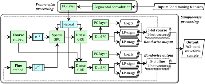
Figure 1: Diagram of the proposed multiband sparse WaveRNN with data-driven linear prediction (MWDLP) using 10-bit mu-law output architecture with coarse and fine bits.

Lastly, to enhance the model capability of handling multispeaker data (universal neural vocoder) as well as of producing high-fidelity output, we propose two novel techniques for discrete waveform modeling. First, we propose to use a data-driven linear prediction (LP) [20] technique for discrete waveform modeling, where the LP coefficients are estimated in a data-driven manner. Secondly, we propose to use loss function based on short-time Fourier transform (STFT) [15] with Gumbel approximation [21] for discrete waveform modeling. These proposed methods are applied on a sparse multiband WaveRNN that utilizes coarse-fine bit architecture for discrete modeling of 10-bit mu-law [22] waveform, which is called multiband WaveRNN with data-driven linear prediction (MWDLP). The experimental results demonstrate that the proposed MWDLP is able to generate high-fidelity synthetic speech for seen and unseen conditions with 300 speakers training data, where each speaker is limited to 60 training utterances, while allowing real-time low-latency usage on low-computational machines, which is, to the best of our knowledge, has never been achieved before.

2 Proposed MWDLP framework for discrete waveform modeling

Let $\bm{{s}}=[s_{1},\dotsc,s_{t_{s}},\dotsc,s_{T_{s}}]^{\top}$ be the sequence of discrete waveform samples and $\bm{{c}}=[\bm{{c}}^{\top}_{1},\dotsc,\bm{{c}}^{\top}_{t_{f}},\dotsc,\bm{{c}}^{\top}_{T_{f}}]^{\top}$ be the sequence of conditioning feature vectors, where $\bm{{c}}_{t_{f}}$ is a $d$-dimensional input feature vector. The sample-level sequence length is denoted as $T_{s}$ and that of frame-level is denoted as $T_{f}$. Consider that the number of bands in multiband processing as $M$, then, the sequence of waveform samples for the $m$th-band is denoted as $\bm{{s}}^{(m)}=[s^{(m)}_{1},\dotsc,s^{(m)}_{t},\dotsc,s^{(m)}_{T_{m}}]^{\top}$, where the length of subband waveform is denoted as $T_{m}=T_{s}/M$. Hence, the sequence of upsampled (repeated) conditioning feature vectors is denoted as $\bm{{c}}^{(u)}=[\bm{{c}}^{(u)^{\top}}_{1},\dotsc,\bm{{c}}^{(u)^{\top}}_{t},\dotsc,\bm{{c}}^{(u)^{\top}}_{T_{m}}]^{\top}$. The objective is to model the probability mass function (p.m.f.) of the discrete waveform as

$$p(\bm{{s}})=\!\prod_{m=1}^{M}\prod_{t=1}^{T_{m}}p(s^{(m)}_{t}|\bm{{c}}^{(u)}_{t}\!,\bm{{s}}^{(M)}_{t-1})=\!\prod_{m=1}^{M}\prod_{t=1}^{T_{m}}\bm{{p}}^{(m)^{\top}}_{t}\!\!\!\bm{{v}}^{(m)}_{t},\!\!$$ (1)

where $\bm{{s}}^{(M)}_{t-1}=[s^{(1)}_{t-1},\dotsc,s^{(m)}_{t-1},\dotsc,s^{(M)}_{t-1}]^{\top}$, $\bm{{p}}^{(m)}_{t}\!\!=\![p^{(m)}_{t}[1],\dotsc,p^{(m)}_{t}[b],\dotsc,p^{(m)}_{t}[B]]^{\top}\!\!\!$, $\bm{{v}}^{(m)}_{t}\!\!=\![v^{(m)}_{t}[1],\dotsc,v^{(m)}_{t}[b],\dotsc,v^{(m)}_{t}[B]]^{\top}\!\!\!$, $\sum_{b=1}^{B}v^{(m)}_{t}[b]\!=\!1$, $v^{(m)}_{t}[b]\!\in\!\{0,\!1\}$, $B$ is the number of sample bins, $\bm{{v}}^{(m)}_{t}$ is a 1-hot vector, and $\bm{{p}}^{(m)}_{t}$ is a probability vector (network output).

2.1 Data-driven LP for discrete modeling

In this work, we propose to use a data-driven LP [20] technique to compute the probability vector of discrete sample bins $\bm{{p}}^{(m)}_{t}$ in Eq. (1). Specifically, the probability of each sample bin $p^{(m)}_{t}[b]$ is given by the $\operatorname*{softmax}$ function as follows:

$$p^{(m)}_{t}[b]=\frac{\exp(\hat{o}^{(m)}_{t}[b])}{\sum_{j=1}^{B}\exp(\hat{o}^{(_{m})}_{t}[j])},$$ (2)

where $\exp(\cdot)$ denotes the exponential function, $\hat{o}^{(m)}_{t}[b]$ is the unnormalized probability (logit) of the $b$th sample bin for the $m$th band at time $t$, and the vector of logits containing all sample bins is given as $\hat{\bm{{o}}}^{(m)}_{t}=[\hat{o}^{(m)}_{t}[1],\dotsc,\hat{o}^{(m)}_{t}[b],\dotsc,\hat{o}^{(m)}_{t}[B]]^{\top}$.

Then, the proposed data-driven LP for discrete waveform modeling is formulated as follows:

$$\hat{\bm{{o}}}^{(m)}_{t}=\sum_{k=1}^{K}a^{(m)}_{t}[k]\bm{{v}}^{(m)}_{t-k}+\bm{{o}}^{(m)}_{t},$$ (3)

where the residual logit vector is denoted as $\bm{{o}}^{(m)}_{t}$, the $k$th data-driven LP coefficient of the $m$th band at time $t$ is denoted as $a^{(m)}_{t}[k]$, $k$ denotes the index of LP coefficient, and the total number of coefficients is denoted as $K$. The data-driven LP coefficient vector containing all coefficients for the $m$th band at time $t$ is given as $\bm{{a}}^{(m)}_{t}=[a^{(m)}_{t}[1],\dotsc,a^{(m)}_{t}[k],\dotsc,a^{(m)}_{t}[K]]^{\top}$. In Eq. (3), $\{\bm{{v}}^{(m)}_{t-1},\dotsc,\bm{{v}}^{(m)}_{t-K}\}$ are used as logit basis vectors corresponding to past $K$ discrete waveform samples $\{s_{t-1},\dotsc,s_{t-K}\}$, which are used for LP in the logit space.

2.2 Network architecture

The network diagram of the proposed MWDLP framework for the modeling of 10-bit mu-law waveform is depicted in Fig.1. Conditioning input features are fed into a segmental convolution layer that takes into account $r=5$ previous and $n=1$ succeeding frames to produce a $((r+1+n)\times d)$-dimensional feature vector from $d$-dimensional input feature vectors, which is then passed to a fully connected (FC) layer with $320$-dimensional output and $\operatorname*{ReLU}$ activation. Separate embedding layers with $64$-dimensionality are used to encode 1-hot vectors of 5-bit fine- and 5-bit coarse-parts of the waveform sample, respectively, which are shared between all bands. Sparse GRU has a relatively large number of hidden units ($1184$), while two separate dense GRUs have small number of hidden units ($32$).

Separate dual fully-connected (DualFC) layers are used for the fine- and coarse-bit outputs. Each DualFC layer produces two output channels that are combined by a trainable weighting vector, as in [11], where the weighting vector is activated by $\exp$ function and multiplied by a constant $0.5$. Each output channel of the DualFC consists of the parts that correspond to the data-driven LP vectors $\bm{{a}}^{(M)}_{t}=[\bm{{a}}^{(1)^{\top}}_{t},\dotsc,\bm{{a}}^{(m)^{\top}}_{t},\dotsc,\bm{{a}}^{(M)^{\top}}_{t}]^{\top}$ and to the logit vector $\bm{{o}}^{(M)}_{t}=[\bm{{o}}^{(1)^{\top}}_{t},\dotsc,\bm{{o}}^{(m)^{\top}}_{t},\dotsc,\bm{{o}}^{(M)^{\top}}_{t}]^{\top}$. The output part of the data-driven LP vectors consists of signs (LP-signs) $\bm{{a}}^{(sg_{M})}_{t}=[\bm{{a}}^{(sg_{1})^{\top}}_{t},\dotsc,\bm{{a}}^{(sg_{m})^{\top}}_{t},\dotsc,\bm{{a}}^{(sg_{M})^{\top}}_{t}]^{\top}$, i.e., with hyperbolic tangent ($\tanh$) activation, and of magnitudes (LP-mags) $\bm{{a}}^{(mg_{M})}_{t}=[\bm{{a}}^{(mg_{1})^{\top}}_{t},\dotsc,\bm{{a}}^{(mg_{m})^{\top}}_{t},\dotsc,\bm{{a}}^{(mg_{M})^{\top}}_{t}]^{\top}$, i.e., with $\exp$ activation. The data-driven LP coefficient vector is computed as $\bm{{a}}^{(M)}_{t}=\bm{{a}}^{(sg_{M})}_{t}\odot\bm{{a}}^{(mg_{M})}_{t}$, where $\odot$ denotes the Hadamard product. The last FC layers with $16$-dimensionality input (from the DualFC logits-part output) on $\operatorname*{ReLU}$ activation, $32$-dimensionality output on $\operatorname*{tanhshrink}$ activation ($x-\tanh(x)$), and shared over all bands, produce the residual logit vector $\bm{{o}}^{(m)}_{t}$.

2.3 STFT-based loss function for discrete modeling

In this work, we also propose an additional loss function based on STFT [15] for discrete waveform modeling, where Gumbel sampling [21] method is utilized. Specifically, it is used to obtain a sampled probability vector of each $m$th band at time $t$ $\hat{\bm{{p}}}^{(m)}_{t}=[\hat{p}^{(m)}_{t}[1],\dotsc,\hat{p}^{(m)}_{t}[b],\dotsc,\hat{p}^{(m)}_{t}[B]]^{\top}$, where a sampled probability of each $b$th bin $\hat{p}^{(m)}_{t}[b]$ is given by

$$\hat{p}^{(m)}_{t}[b]=\frac{\exp(\hat{\gamma}^{(m)}_{t}[b])}{\sum_{j=1}^{B}\exp(\hat{\gamma}^{(m)}_{t}[j])},$$ (4)

In Eq. (4), $\hat{\gamma}^{(m)}_{t}[b]$ denotes a sampled logit, where a sampled logit vector $\hat{\bm{{\gamma}}}^{(m)}_{t}=[\hat{\gamma}^{(m)}_{t}[1],\dotsc,\hat{\gamma}^{(m)}_{t}[b],\dotsc,\hat{\gamma}^{(m)}_{t}[B]]^{\top}$ is computed as

$$\hat{\bm{{\gamma}}}^{(m)}_{t}=\hat{\bm{{o}}}^{(m)}_{t}-\log(-\log(\bm{{u}})),\text{s. t.}\>\bm{{u}}\sim(0,1),$$ (5)

and $\bm{{u}}$ is a uniformly distributed $B$-dimensional vector.

Then, the discrete value of the sampled waveform bin $\hat{s}^{(m)}_{t}$ can be recovered while keeping the backpropagation path from the reparameterization with Gumbel sampling in Eq. (5) as

$$\hat{s}^{(m)}_{t}=f\bigg{(}\sum_{b=1}^{B}\>b\>\>\overline{\hat{p}}^{(m)}_{t}[b]\bigg{)},\>\>\text{s. t.}$$

$$\overline{\hat{p}}^{(m)}_{t}[b] =\begin{cases}\frac{\hat{p}^{(m)}_{t}[b]}{\max{(\hat{\bm{{p}}}^{(m)}_{t})}},&\!\!\text{if}\>\>\hat{p}^{(m)}_{t}[b]=\max{(\hat{\bm{{p}}}^{(m)}_{t})},\\ 0,&\!\!\text{else,}\end{cases}$$ (6)

where $\max(\bm{{p}})$ is a function that returns the maximum value of a vector $\bm{{p}}$ and $f(b)$ denotes a differentiable function that returns the waveform value of a discrete sample bin $b$, e.g., an inverse mu-law [22] function. Hence, the STFT-based loss is computed from the sampled waveform $\hat{\bm{{s}}}^{(m)}=[\hat{s}^{(m)}_{1},\dotsc,\hat{s}^{(m)}_{t},\dotsc,\hat{s}^{(m)}_{T_{m}}]^{\top}$ and the target waveform $\bm{{s}}^{(m)}$ as

$$\mathcal{L}_{\text{STFT}}^{(m)}=g(\operatorname*{STFT}(\bm{{\hat{s}}}^{(m)}),\operatorname*{STFT}(\bm{{s}}^{(m)})),$$ (7)

where $\operatorname*{STFT}(\cdot)$ denotes an STFT analysis function that produces frames of complex STFT spectra and $g(\cdot,\cdot)$ denotes a set of STFT-based loss functions. Ultimately, the loss of full-band waveform $\bm{{s}}$ can also be computed as in [23]. Note that the discretization through thresholding with $\max(\cdot)$ function in Eq. (6) is necessary to accommodate the $f(\cdot)$ function.

2.4 Sparsification and model complexity

In training, a sparsification procedure is performed for the recurrent matrices of the large sparse $1184$ GRU in Fig. (1), where the average target density from all recurrent matrices of update, reset, and new gates [19, 11] is $0.1$, and each target densities are $0.09$, $0.09$, and $0.12$, respectively. The complexity is computed as in [11, 17] with adjustments according to the MWDLP architecture. For a 24 kHz waveform model with $M=6$ bands and $K=8$ LP coefficients, the total complexity of the band-rate module is $\sim\,\!\!4.53$ GFLOPS, while for a 16 kHz model with $M=4$ and $K=8$, it is $\sim\,\!\!4.24$ GFLOPS.

Table 1: Training/Development speech dataset configurations. The number of training utterances per speaker is limited to $60$.

Language/dialect/condition	# Male	# Female
Spanish (4 dialects) [24]	$20$	$20$
Catalan, Galician [25]	$10$	$10$
Yoruba [26], isiXhosa [27]	$5$	$12$
Gujarati, Marathi [28]	$5$	$14$
Tamil, Telugu [28]	$10$	$10$
Bengali (Bangladeshi, Indian) [29]	$13$	$1$
Javanese, Khmer [29]	$5$	$15$
French (Emotional/Expressive) [30]	$4$	$4$
Japanese [31]	$29$	$29$
English [32]	$28$	$28$
English (Noisy/Reverberant) [33]	$14$	$14$

Table 2: Real-time factor (RTF) of MWDLP with $4$ kHz resolution per band and $8$ data-driven LP coefficients, which includes input/output and feature extraction (I/O + feat.).

RTF w/ I/O + feat. on 1-core CPU	16 kHz	24 kHz
Intel® Xeon® Gold 6230 $2.1$ GHz	$0.58$	$0.64$
Intel® Xeon® Gold 6142 $2.6$ GHz	$0.57$	$0.63$
Intel® Core™ i7-7500U $2.7$ GHz	$0.57$	$0.63$

3 Experimental evaluation

3.1 Experimental conditions

We used speech data from $300$ speakers [24, 25, 26, 27, 28, 29, 30, 31, 32] consisting of over $18$ languages/dialects including few expressive speech data and noisy/reverberant speech data. The number of training utterances per speaker was limited to $60$ and the number of development utterances per speaker was $5$, which were used for early stopping. The details of the training/development speech dataset are given in Table 1. Additionaly, for evaluation on unseen conditions, we also utilized speech data of another $3$ speakers/languages: a male Basque [25], a female Malayalam [28], and a female Chinese [5] speakers.

For the proposed MWDLP framework, as the conditioning input feature, we utilized $80$-dimensional mel-spectrogram, which was extracted from the STFT magnitude spectra. In STFT analysis, the shift length was set to $10$ ms, the window length was set to $27.5$ ms, and Hanning window was used. For $24$ kHz waveform, the FFT length was set to $2048$, while for $16$ kHz waveform, it was set to $1024$. The ablation objective evaluation was performed using the $24$ kHz models.

Table 3: Objective evaluation results excluding noisy/reverberant data with variations of data-driven linear prediction (LP) and the use of STFT loss (STFT).

Model	MCD [dB]	U/V [%]	F0 [Hz]	LSD [dB]
MWDLP 0LP	$2.88$	$12.17$	$17.28$	$4.93$
MWDLP 0LP+STFT	$2.97$	$12.18$	$17.67$	$5.05$
MWDLP 6LP	$2.87$	$13.17$	$17.53$	$4.95$
MWDLP 6LP+STFT	$2.91$	$13.03$	$17.51$	$4.93$
MWDLP 8LP	$2.87$	$12.33$	$17.25$	$4.82$
MWDLP 8LP+STFT	2.78	12.10	17.25	4.80
PWG	2.88	15.44	20.07	4.49
Fatchord	$6.03$	$27.60$	$17.22$	$7.32$
LPCNet	$4.09$	$13.50$	$21.82$	$11.92$

The hyperparameters of MWDLP were set as in Sections 2.2 and 2.4. In training, dropout with $0.5$ probability was used after the upsampling (repetition) of conditioning input features. RAdam [34] algorithm was used for the parameter optimization, where the learning rate was set to $0.0001$. Weight normalization [35] was used for convolution and fully-connected layers. The batch sequence length was set to $6$ frames and the batch size was set to $8$. Using a single NVIDIA RTX 2080Ti, the training time for a $24$ kHz model with a number of bands $M=6$, a number of data-driven LP $K=8$ (Section 2.1), and $5$ windowing configurations for the STFT-based loss (Section 2.3) was $\sim\!4.8$ days. On the other hand, the real-time factor (RTF) in synthesis was $0.57$–$0.64$ including input/output and feature extraction, which was obtained using a single core of $2.1$–$2.7$ GHz CPU as given in Table 2. The footprint size of the compiled model, i.e., the executable, was $16$ MB. The software has been made available at https://github.com/patrickltobing/cyclevae-vc-neuralvoco.

The number of data-driven LP coefficients $K$ was varied to $\{0,6,8\}$. In [36], it was recommended to use one coefficient per kHz plus two pairs of coefficients, each for spectral slope and voice quality, which puts $K=8$ to be the most suitable for a MWDLP model with $4$ kHz band-waveform resolution. The $5$ windowing configurations for the STFT-based loss were set for each band-resolution and full-band waveforms. On full-band, the FFT lengths were set to $\{2048,1024,512,256,128\}$ for $24$ kHz and $\{1024,512,256,128,128\}$ for $16$ kHz, while the shift lengths were set to $\{480,240,120,60,48\}$ for $24$ kHz and to $\{320,160,80,40,32\}$ for $16$ kHz. On band-waveform, the FFT lengths were set to $\{256,128,64,32,32\}$ and the shift lengths were set to $\{80,40,20,10,8\}$. In all cases, the window lengths were set to $2.5$ multiple of the shift lengths.

Pseudo-quadratic mirror filter (PQMF) [37] was used for the multiband analysis and synthesis [17]. The Kaiser prototype filter configurations were as follows: the order was set to $410$ for $24$ kHz or to $274$ for $16$ kHz, the $\beta$ coefficient was set to $43.12126$, and the cutoff ratio was set to $0.1$ for $24$ kHz or to $0.15$ for $16$ kHz. Pre-emphasis with $\alpha=0.85$ was applied to the full-band waveform before PQMF analysis.

Lastly, for additional baselines, we also developed $24$ kHz waveform models with a publicly available WaveRNN implementation https://github.com/fatchord/WaveRNN (Fatchord) and with Parallel WaveGAN (PWG) [15], which is a non-AR neural vocoder, and a $16$ kHz model using LPCNet [11]. The training sets were the same as for MWDLP, given in Table 1.

Table 4: Objective evaluation results on noisy/reverberant data. Number of data-driven linear prediction (LP) was varied including the use of STFT loss (STFT).

Model	MCD [dB]	LSD [dB]
MWDLP 0LP	$2.90$	$4.37$
MWDLP 0LP+STFT	$2.48$	$4.24$
MWDLP 6LP	$2.79$	$4.88$
MWDLP 6LP+STFT	$2.49$	$4.60$
MWDLP 8LP	$2.57$	$4.19$
MWDLP 8LP+STFT	2.44	4.04
PWG	2.41	4.16
Fatchord	$3.49$	$4.84$
LPCNet	$3.33$	$5.40$

3.2 Objective evaluation

In the objective evaluation, we measured the mel-cepstral distortion (MCD) [38], unvoiced/voiced decision error (U/V), root-mean-square error of fundamental frequency (F0), and log spectral distortion (LSD). On the measurements of MCD, U/V, and F0 accuracies, WORLD [7] was used to extract F0 and spectral envelope, where $28$-dimensional mel-cepstral coefficients were extracted with $0.466$ frequency warping for $24$ kHz and $0.41$ for $16$ kHz. For log-spectral distortion, $80$-dimensional mel-spectrogram extracted from the magnitude spectra as in Section 3.1 was used. To adjust for the phase differences between synthesized and target waveforms, dynamic-time-warping was computed with respect to the extracted mel-cepstra. $9969$ and $9752$ testing utterances were used for evaluation without and with noisy/reverberant speech, respectively.

The result of objective evaluation without noisy/reverberant speech test set is given in Table 3. It can be observed that the use of $8$ data-driven LP provides better accuracies on all MCD, U/V, F0, and LSD compared to without using data-driven LP and with $6$ data-driven LP. The use of STFT-based loss further improves the model with $8$ data-driven LP yielding the best accuracies on MCD, U/V, F0 and LSD with values of $2.78$ dB, $12.10~{}\!\%$, $17.25$ Hz and $4.80$ dB, respectively. On the other hand, the result of objective evaluation with noisy/reverberant speech test set is given in Table 4, where U/V and F0 measurements were reasonably omitted. In this result, it can be observed that the use of $8$ data-driven LP also provides better MCD and LSD values compared to without using data-driven LP or $6$ data-driven LP, while the use of STFT-based loss further improves it to yield the best MCD and LSD with values of $2.44$ dB and $4.04$ dB, respectively. Lower values on noisy/reverberant test set are mainly due to the non-existence of silent speech regions, especially for LPCNet model, where it tends to produce unclear/noisy sounds and for Fatchord model, where it generates too much noise/artifact even for clean speech. Overall, it has been shown that the tendency of consistent improvements is obtained by the proposed MWDLP with $8$ data-driven LP using STFT-based loss (MWDLP 8LP+STFT). Our preliminary testing by listening on the speech samples also suggests that the MWDLP 8LP+STFT provides the highest speech quality.

Table 5: Subjective evaluation results showing mean opinion score (MOS) from seen and unseen sets.

Model – MOS	Seen	Unseen	All
Original $24$ kHz	$4.56\pm 0.07$	$4.57\pm 0.07$	$4.57\pm 0.05$
Original $16$ kHz	$4.47\pm 0.09$	$4.56\pm 0.09$	$4.52\pm 0.06$
MWDLP $24$ kHz	$\bm{4.15\pm 0.09}$	$\bm{4.29\pm 0.09}$	$\bm{4.22\pm 0.06}$
MWDLP $16$ kHz	$\bm{3.98\pm 0.09}$	$\bm{4.29\pm 0.09}$	$\bm{4.13\pm 0.06}$
PWG $24$ kHz	$3.93\pm 0.11$	$4.20\pm 0.10$	$4.07\pm 0.07$
Fatchord $24$ kHz	$2.11\pm 0.11$	$2.13\pm 0.13$	$2.12\pm 0.08$
LPCNet $16$ kHz	$3.14\pm 0.11$	$3.22\pm 0.10$	$3.18\pm 0.08$

3.3 Subjective evaluation

In the subjective evaluation, we chose the MWDLP 8LP+STFT configurations for the $16$ and $24$ kHz waveform models, which were also compared with the Fatchord $24$ kHz and LPCNet $16$ kHz models, as well as the original $16$  and $24$ kHz waveforms. The number of evaluated speakers from the seen dataset of Table 1 was 3, which were a Spanish Female (Argentinian) [24], a Yoruba male [26], and an English male [32] speakers. The number of evaluated unseen speakers/language was $3$ as given in Section 3.1. The number of testing utterances per speaker was $10$, i.e., a total of $60$ listening web-pages. Corresponding languages of the audios were also shown to the listeners. The number of crowd-sourced listeners from Amazon Mechanical Turk was $20$.

The subjective evaluation result is shown in Table 5, where the $5$-scaled mean opinion score (MOS) values on the speech quality ranging from $1$ (very bad) to $5$ (very good) are given. It can be clearly observed that the proposed MWDLP gives the best performances compared to the $24$ kHz and $16$ kHz baseline models by achieving MOS values of $4.15$ and $4.29$ on seen and unseen data, respectively, for $24$ kHz model and of $3.98$ and $4.29$ on seen and unseen data, respectively, for $16$ kHz model. It can also be observed that the scores of seen speakers are lower than unseen speakers, which is due to the better recording quality for the evaluated unseen speakers. Note that the only systems that can be run real-time with low-latency processing on CPU are the proposed MWDLP and LPCNet [11]. Samples and demo are available at https://demo-mwdlp-interspeech2021.audioeval.net.

4 Conclusions

We have presented a novel real-time low-latency universal neural vocoder with high-fidelity output based on multiband WaveRNN using data-driven linear prediction for discrete waveform modeling (MWDLP). The proposed MWDLP framework utilizes a relatively large number of hidden units for the main RNN module, where sparsification and multiband modeling approaches are applied to reduce the effective model size and the model complexity. A novel data-driven linear prediction (LP) technique is proposed for the use in discrete waveform modeling, where the LP coefficients are estimated in a data-driven manner. Further, a novel approach for short-time Fourier transform (STFT)-based loss computation on discrete modeling with Gumbel approximation is also proposed. The results have demonstrated that the MWDLP framework is able to generate high-fidelity synthetic speech, where it is trained with a $300$ speakers dataset, with $0.57$–$0.64$ real-time factor using a single-core of $2.1$–$2.7$ GHz CPU.

5 Acknowledgements

This work was partly supported by JSPS KAKENHI Grant Number 17H06101 and JST, CREST Grant Number JPMJCR19A3.

References

- [1] A. Tamamori, T. Hayashi, K. Kobayashi, K. Takeda, and T. Toda, “Speaker-dependent WaveNet vocoder,” in Proc. INTERSPEECH, Stockholm, Sweden, Aug. 2017, pp. 1118–1122.
- [2] Y. Ai, H.-C. Wu, and Z.-H. Ling, “SampleRNN-based neural vocoder for statistical parametric speech synthesis,” in Proc. ICASSP, Calgary, Canada, Apr. 2018, pp. 5659–5663.
- [3] A. Oord, Y. Li, I. Babuschkin, K. Simonyan, O. Vinyals, K. Kavukcuoglu, G. Driessche, E. Lockhart, L. Cobo, F. Stimberg, and N. Casagrande, “Parallel WaveNet: Fast high-fidelity speech synthesis,” in Proc. ICML, Stockholm, Sweden, Jul. 2018, pp. 3918–3926.
- [4] J. Shen, R. Pang, R. J. Weiss, M. Schuster, N. Jaitly, Z. Yang, Z. Chen, Y. Zhang, Y. Wang, R. J. Skerry-Ryan, R. A. Saurous, Y. Agiomyrgiannakis, and Y. Wu, “Natural TTS synthesis by conditioning WaveNet on mel spectrogram predictions,” in Proc. ICASSP, Calgary, Canada, Apr. 2018, pp. 4779–4783.
- [5] Y. Zhao, W.-C. Huang, X. Tian, J. Yamagishi, R. K. Das, T. Kinnunen, Z. Ling, and T. Toda, “Voice Conversion Challenge 2020 intra-lingual semi-parallel and cross-lingual voice conversion,” in ISCA Joint Workshop for the Blizzard Challenge and Voice Conversion Challenge 2020, Shanghai, China, Oct. 2020, pp. 80–98.
- [6] H. Kawahara, I. Masuda-Katsuse, and A. De Cheveigné, “Restructuring speech representations using a pitch-adaptive time-frequency smoothing and an instantaneous-frequency-based F0 extraction: Possible role of a repetitive structure in sounds,” Speech Commun., vol. 27, pp. 187–207, 1999.
- [7] M. Morise, F. Yokomori, and K. Ozawa, “WORLD: A vocoder-based high-quality speech synthesis system for real-time applications,” IEICE Trans. Inf. Syst., vol. 99, no. 7, pp. 1877–1884, 2016.
- [8] A. v. d. Oord, S. Dieleman, H. Zen, K. Simonyan, O. Vinyals, A. Graves, N. Kalchbrenner, A. Senior, and K. Kavukcuoglu, “WaveNet: A generative model for raw audio,” arXiv preprint arXiv:1609.03499, 2016.
- [9] N. Kalchbrenner, E. Elsen, K. Simonyan, S. Noury, N. Casagrande, E. Lockhart, F. Stimberg, A. v. d. Oord, S. Dieleman, and K. Kavukcuoglu, “Efficient neural audio synthesis,” arXiv preprint arXiv:1802.08435, 2018.
- [10] Z. Jin, A. Finkelstein, G. Mysore, and J. Lu, “FFTNet: A real-time speaker-dependent neural vocoder,” in Proc. ICASSP, Calgary, Canada, Apr. 2018, pp. 2251–2255.
- [11] J.-M. Valin and J. Skoglund, “LPCNet: Improving neural speech synthesis through linear prediction,” in Proc. ICASSP, Brighton, UK, May 2019, pp. 5891–5895.
- [12] X. Wang, S. Takaki, and J. Yamagishi, “Neural source-filter-based waveform model for statistical parametric speech synthesis,” in Proc. ICASSP, Brighton, UK, May 2019, pp. 5916–5920.
- [13] R. Prenger, R. Valle, and B. Catanzaro, “WaveGlow: A flow-based generative network for speech synthesis,” in Proc. ICASSP, Brighton, UK, May 2019, pp. 3617–3621.
- [14] K. Kumar, R. Kumar, T. de Boissiere, L. Gestin, W. Z. Teoh, J. Sotelo, A. de Brébisson, Y. Bengio, and A. C. Courville., “MelGAN: Generative adversarial networks for conditional waveform synthesis,” in Advances in Neural Inf. Process. Syst., 2019, pp. 14 910–14 921.
- [15] R. Yamamoto, E. Song, and J.-M. Kim, “Parallel WaveGAN: A fast waveform generation model based on generative adversarial networks with multi-resolution spectrogram,” in Proc. ICASSP, Barcelona, Spain, May 2020, pp. 6199–6203.
- [16] T. Okamoto, T. Toda, Y. Shiga, and H. Kawai, “Improving FFTNet vocoder with noise shaping and subband approaches,” in Proc. SLT, Athens, Greece, Dec. 2018, pp. 304–311.
- [17] C. Yu, H. Lu, N. Hu, M. Yu, C. Weng, K. Xu, P. Liu, D. Tuo, S. Kang, G. Lei et al., “DurIAN: Duration informed attention network for multimodal synthesis,” arXiv preprint arXiv:1909.01700, 2019.
- [18] Q. Tian, Z. Zhang, H. Lu, L.-H. Chen, and S. Liu, “FeatherWave: An efficient high-fidelity neural vocoder with multi-band linear prediction,” arXiv preprint arXiv:2005.05551, 2020.
- [19] K. Cho, B. Van Merriënboer, C. Gulcehre, D. Bahdanau, F. Bougares, H. Schwenk, and Y. Bengio, “Learning phrase representations using RNN encoder-decoder for statistical machine translation,” arXiv preprint arXiv:1406.1078, 2014.
- [20] B. S. Atal and S. L. Hanauer, “Speech analysis and synthesis by linear prediction of the speech wave,” J. Acoust. Soc. Amer., vol. 50, no. 2B, pp. 637–655, 1971.
- [21] C. J. Maddison, D. Tarlow, and T. Minka, “A* sampling,” arXiv preprint arXiv:1411.0030, 2014.
- [22] ITUT-Recommendation, “G. 711: Pulse code modulation of voice frequencies,” 1988.
- [23] G. Yang, S. Yang, K. Liu, P. Fang, W. Chen, and L. Xie, “Multi-band MelGAN: Faster waveform generation for high-quality text-to-speech,” arXiv preprint arXiv:2005.05106, 2020.
- [24] A. Guevara-Rukoz, I. Demirşahin, F. He, S.-H. C. Chu, S. Sarin, K. Pipatsrisawat, A. Gutkin, A. Butryna, and O. Kjartansson, “Crowdsourcing Latin American Spanish for low-resource text-to-speech,” in Proc. LREC, Marseille, France, May 2020, pp. 6504–6513.
- [25] O. Kjartansson, A. Gutkin, A. Butryna, I. Demirşahin, and C. Rivera, “Open-source high quality speech datasets for Basque, Catalan and Galician,” in Proc. SLTU and CCURL, Marseille, France, May 2020, pp. 21–27.
- [26] A. Gutkin, I. Demirşahin, O. Kjartansson, C. Rivera, and K. Túbòsún, “Developing an open-source corpus of Yoruba speech,” Shanghai, China, Oct. 2020, pp. 404–408.
- [27] D. van Niekerk, C. van Heerden, M. Davel, N. Kleynhans, O. Kjartansson, M. Jansche, and L. Ha, “Rapid development of TTS corpora for four South African languages,” Stockholm, Sweden, Aug. 2017, pp. 2178–2182.
- [28] F. He, S.-H. C. Chu, O. Kjartansson, C. Rivera, A. Katanova, A. Gutkin, I. Demirşahin, C. Johny, M. Jansche, S. Sarin, and K. Pipatsrisawat, “Open-source multi-speaker speech corpora for building Gujarati, Kannada, Malayalam, Marathi, Tamil and Telugu speech synthesis systems,” in Proc. LREC, Marseille, France, May 2020, pp. 6494–6503.
- [29] K. Sodimana, P.-D. Silva, S. Sarin, O. Kjartansson, M. Jansche, K. Pipatsrisawat, and L. Ha, “A step-by-step process for building TTS voices using open source data and frameworks for Bangla, Javanese, Khmer, Nepali, Sinhala, and Sundanese,” in Proc. SLTU, Gurugram, India, Aug. 2018, pp. 66–70.
- [30] C. Le Moine and N. Obin, “Att-HACK: An expressive speech database with social attitudes,” in Proc. Speech Prosody, Tokyo, Japan, May 2020, pp. 744–748.
- [31] S. Takamichi, K. Mitsui, Y. Saito, T. Koriyama, N. Tanji, and H. Saruwatari, “JVS corpus: free Japanese multi-speaker voice corpus,” arXiv preprint arXiv:1908.06248, 2019.
- [32] C. Veaux, J. Yamagishi, and K. MacDonald, “Superseded-CSTR VCTK corpus: English multi-speaker corpus for CSTR voice cloning toolkit,” 2016.
- [33] C. Valentini-Botinhao, “Noisy reverberant speech database for training speech enhancement algorithms and TTS models,” 2017.
- [34] L. Liu, H. Jiang, P. He, W. Chen, X. Liu, J. Gao, and J. Han, “On the variance of the adaptive learning rate and beyond,” arXiv preprint arXiv:1908.03265, 2019.
- [35] T. Salimans and D. P. Kingma, “Weight normalization: A simple reparameterization to accelerate training of deep neural networks,” arXiv preprint arXiv:1602.07868, 2016.
- [36] J. D. Markel and A. H. Gray, Linear prediction of speech. Springer-Verlag, Berlin, 1976.
- [37] T. Q. Nguyen, “Near-perfect-reconstruction pseudo-QMF banks,” IEEE Trans. Sig. Process., vol. 42, no. 1, pp. 65–76, 1994.
- [38] M. Mashimo, T. Toda, K. Shikano, and N. Campbell, “Evaluation of cross-language voice conversion based on GMM and STRAIGHT,” in Proc. EUROSPEECH, Aalborg, Denmark, Sep. 2001.