Lookahead Acquisition Functions for Finite-Horizon Time-Dependent Bayesian Optimization and Application to Quantum Optimal Control

Abstract

We propose a novel Bayesian method to solve the maximization of a time-dependent expensive-to-evaluate stochastic oracle. We are interested in the decision that maximizes the oracle at a finite time horizon, given a limited budget of noisy evaluations of the oracle that can be performed before the horizon. Our recursive two-step lookahead acquisition function for Bayesian optimization makes nonmyopic decisions at every stage by maximizing the expected utility at the specified time horizon. Specifically, we propose a generalized two-step lookahead framework with a customizable value function that allows users to define the utility. We illustrate how lookahead versions of classic acquisition functions such as the expected improvement, probability of improvement, and upper confidence bound can be obtained with this framework. We demonstrate the utility of our proposed approach on several carefully constructed synthetic cases and a real-world quantum optimal control problem.

1 Introduction

We consider the maximization of an expensive-to-evaluate oracle $f(\mathbf{x},t)$, where $\mathbf{x}\in\bm{\mathcal{X}}\subset\mathbb{R}^{d}$ are the inputs or action parameters in a compact domain and $t$ is the context from a (possibly infinite) set of contexts $\mathcal{T}$. An observation $\hat{y}\in\mathbb{R}$ made by observing $f$ at the action-context pair $(\mathbf{x},t)$ is assumed to be corrupted by additive stochastic noise $\epsilon$; that is, $\hat{y}=f(\mathbf{x},t)+\epsilon$. Furthermore, we assume a context space $\mathcal{T}$ whose members have a unique ordering (hereafter “time”). We seek an action $\mathbf{x}^{*}_{T}$ at a given future time $T\in\mathcal{T}$ that solves

$$\operatornamewithlimits{arg\,max}_{\mathbf{x}\in\bm{\mathcal{X}}}f(\mathbf{x},T)$$ (1)

in as few stochastic observations of $f$ as possible. Such a problem fundamentally differs from general context-dependent bandit problems [17, 31] in that we are interested solely in the action that maximizes the oracle value $f$ at time $t=T$, as opposed to maximizing the cumulative oracle value until $T$. Additionally, we assume that only one observation can be made per time $t$. The time-dependent maximization that we address arises, for example, in quantum computing and control [21, 42], where values for the control parameter $\mathbf{x}$ are sought by using noisy observations $f(\mathbf{x},t)$ to achieve a desired task at future time $T$; see section 5.3. Another application relevant to our work is multistage stochastic programming for portfolio optimization [28, Ch. 1], where the goal is to find a policy $\{(\mathbf{x}_{i},t_{i}):~{}i=0,\ldots,n-1\}$ for redistributing assets to maximize the expected profit at $T=t_{n}$ and the profit at each stage is realized by querying a noisy oracle. In many settings, $\bm{\mathcal{X}}$ is a simple domain; here we assume that $\bm{\mathcal{X}}:=[0,1]^{d}$ so that the inputs $\mathbf{x}$ are normalized.

The main challenges of the problem (1) that we seek to address are (i) the absence of structure (e.g., convexity) in $f$ that could potentially be exploited, (ii) the high cost associated with each observation of $f$, and (iii) the time-varying setting where observations of $f$ cannot be made in the past or future. Bayesian optimization (BO) [5, 27] with Gaussian process (GP) priors [12, 26] suits the specific challenges posed by our problem (mainly (i) and (ii) mentioned above), where observations at each round $i$, $\hat{y}_{i}=f(\mathbf{x}_{i},t_{i})+\epsilon_{i}$, are made judiciously by leveraging information gained from previous observations, as a means of coping with the high costs of each observation. The key idea is to specify GP prior distributions on the oracle value and the noise. That is, $f(\mathbf{x},t)\sim\mathcal{GP}\left(0,k((\mathbf{x},t),(\mathbf{x}^{\prime},t^{\prime}))\right)$ and $\epsilon\sim\mathcal{GP}(0,\sigma^{2}_{\epsilon})$, where $\sigma^{2}_{\epsilon}$ is a constant noise variance. The covariance function $k$ captures the correlation between the observations in the joint $(\mathbf{x},t)$ space; here we use the product composite form given by $k((\mathbf{x},t),(\mathbf{x}^{\prime},t^{\prime}))=k_{\mathbf{x}}(\mathbf{x},\mathbf{x}^{\prime};\theta_{\mathbf{x}})\times k_{t}(t,t^{\prime};\theta_{t})$, where $\theta_{\mathbf{x}}$ and $\theta_{t}$ parameterize the covariance functions for $\mathbf{x}$ and $t$, respectively. We estimate the GP hyperparameters $\bm{\Omega}=\{\theta_{x},\theta_{t},\sigma^{2}_{\epsilon}\}$ from data by maximizing the marginal likelihood. We use the squared-exponential kernels defined as $k_{\mathbf{x}}(\mathbf{x},\mathbf{x}^{\prime})=\textnormal{exp}\left(-\frac{\|\mathbf{x}-\mathbf{x}^{\prime}\|^{2}}{2\theta^{2}_{\mathbf{x}}}\right)$ and $k_{t}(t,t^{\prime})=\textnormal{exp}\left(-\frac{\|t-t^{\prime}\|^{2}}{2\theta^{2}_{t}}\right)$. The posterior predictive distribution of the output $Y$, conditioned on available observations from the oracle, is given by

$$\begin{split}Y(\mathbf{x},t|\bm{\mathcal{D}}_{n},\bm{\Omega})&\sim\mathcal{GP}(\mu_{n}(\mathbf{x},t),\sigma^{2}_{n}(\mathbf{x},t)),~{}\quad\bm{\mathcal{D}}_{n}:=\{(\mathbf{x}_{i},t_{i}),\hat{y}_{i}\}_{i=1}^{n}\\ \mu_{n}(\mathbf{x},t)&=\mathbf{k}_{n}^{\top}[\mathbf{K}_{n}+\sigma_{\epsilon}^{2}\mathbf{I}]^{-1}\mathbf{y}_{n}\\ \sigma^{2}_{n}(\mathbf{x},t)&=k((\mathbf{x},t),(\mathbf{x},t))-\mathbf{k}_{n}^{\top}[\mathbf{K}_{n}+\sigma_{\epsilon}^{2}\mathbf{I}]^{-1}\mathbf{k}_{n},\end{split}$$ (2)

where $\mathbf{k}_{n}$ is a vector of covariances between $(\mathbf{x},t)$ and all observed points in $\bm{\mathcal{D}}_{n}$, $\mathbf{K}_{n}$ is a sample covariance matrix of observed points in $\bm{\mathcal{D}}_{n}$, $\mathbf{I}$ is the identity matrix, and $\mathbf{y}_{n}$ is the vector of all observations in $\bm{\mathcal{D}}_{n}$; (2) is then used as a surrogate model for $f$ in Bayesian optimization. Note that $\mu_{n}$ and $\sigma_{n}^{2}$ are the posterior mean and variance of the GP, respectively, where the subscript $n$ implies the conditioning based on $n$ past observations. BO then proceeds by defining an acquisition function, $\alpha(\mathbf{x},t)$, in terms of the GP posterior that is optimized in lieu of the expensive $f$ to select the next point $\mathbf{x}_{n+1}$ at $t_{n+1}$, and the process continues until a budget of $q$ observations is reached; see Algorithm 1. We denote by $\mathbf{x}_{i}$ and $\mathbf{x}_{t}$ a decision made by maximizing the acquisition function at $t_{i}$ and $t$, respectively. We use $\mathbf{x}_{t}^{*}$ to denote a maximizer of $f(\cdot,t)$.

1 Given: $\bm{\mathcal{D}}_{n}=\{(\mathbf{x}_{i},t_{i}),\hat{y}_{i}\}_{i=1}^{n}$, total budget $q$, schedule $\{t_{n+1},\ldots,t_{q}=T\}$, and GP hyperparameters $\bm{\Omega}$

Result: $(\mathbf{x}_{T},\hat{y}_{T})$

2 for $i=n+1,\ldots,q$,  do

3       Find $\mathbf{x}_{i}\in\underset{\mathbf{x}\in\bm{\mathcal{X}}}{\operatornamewithlimits{arg\,max}}~{}\alpha(\mathbf{x},t_{i})$   (acquisition function maximization based on $\bm{\Omega}$)

4       Observe $\hat{y}_{i}$ = $f(\mathbf{x}_{i},t_{i})+\epsilon_{i}$

5       Append $\bm{\mathcal{D}}_{i}=\bm{\mathcal{D}}_{i-1}\cup\{(\mathbf{x}_{i},t_{i}),\hat{y}_{i}\}$

6       Update GP hyperparameters $\bm{\Omega}$

7      

Algorithm 1 Generic Bayesian optimization

Typical acquisition functions in BO take a greedy (“myopic”) approach, where each $\mathbf{x}_{i}$ is selected as though it were the last, without accounting for the potential impact on future selections. Such myopic acquisition functions include the probability of improvement (PI) [18], the expected improvement (EI) [15, 22], and the GP upper confidence bound (UCB) [31], which are, respectively,

$$\begin{split}\alpha_{\textrm{PI}}(\mathbf{x},t)&=\Phi\left(z\right)\\ \alpha_{\textrm{EI}}(\mathbf{x},t)&=z\sigma_{n}(\mathbf{x},t)\Phi\left(z\right)+\sigma_{n}(\mathbf{x},t)\phi\left(z\right)\\ \alpha_{\textrm{UCB}}(\mathbf{x},t)&=\mu_{n}(\mathbf{x},t)+\beta^{1/2}\sigma_{n}(\mathbf{x},t),\end{split}$$ (3)

where $z=\frac{\mu_{n}(\mathbf{x},t)-\xi}{\sigma_{n}(\mathbf{x},t)}$; $\Phi$ and $\phi$ denote the standard normal cumulative and probability density functions, respectively; $\xi$ is a user-specified target; and $\beta$ is a confidence parameter. Whereas the PI and EI acquisition functions are probabilistic measures of improvement over a user-specified target, UCB is an optimistic estimate. Under suitable regularity conditions, the PI, EI, and UCB acquisition functions are guaranteed to achieve asymptotic consistency [6, 22, 31, 34] in BO. For a limited budget $q$, however, such acquisition functions can be suboptimal [11]. Furthermore, the myopic nature of these basic acquisition functions is such that they seek to maximize the oracle value at $t=T$ only when they arrive at $T$, meaning that the past ($t<T$) decisions are not necessarily made to facilitate making the best decision for $t=T$. On the other hand, we are interested in a strategy that seeks to maximize $f(\mathbf{x},T)$. Since the time horizon $t=T<\infty$, this is a finite-horizon problem.

For time-dependent objectives, an optimal decision may be horizon-dependent, which poses a challenge for improvement-based acquisition functions such as PI and EI. Because the target $\xi$ is typically chosen as the best observed value in $\{\hat{y}_{i}\}_{i=1}^{n}$, specifying an appropriate target when the maximum oracle value $\max f(\mathbf{x},t)$ changes with time $t$ is challenging. For example, what if the maximum oracle value at $T$ is much smaller than anything observed until current time $t$? A further challenge in our context is that observations at the target time $T$ are not realizable until we conclude the optimization. Therefore, in such situations, myopic acquisition functions that seek the best oracle value at the current $t$ may not necessarily be useful. Instead, we are interested in acquisition functions that optimize the long-sighted decision (at $t=T$) even if it means incurring a suboptimal oracle value at intermediate $t<T$. In the BO literature, strategies that make decisions by accounting for the decisions remaining in the future are generally referred to as lookahead approaches, which we adopt to solve our finite-horizon problem.

We now illustrate the benefit of a lookahead acquisition function in the context of time-dependent BO. Figure 1 shows the difference between the decisions made via EI and the lookahead acquisition function 2LEY introduced in section 2. The top left of the figure shows contours of the true (noise-free) oracle with a target horizon of $T=3.0$. We assume we have made $n$ decisions before $t_{n+1}=2.625$, and we are interested in making a decision at current $t_{n+1}$ (denoted by the horizontal dashed line). The top right shows the 2LEY and EI acquisition functions and the corresponding decisions made by maximizing each of them (denoted by vertical dashed lines). In the bottom row, we show the GP predictions at $T$, with each of the decisions made via the myopic and lookahead acquisition functions incorporated, along with the noise-free $f(\mathbf{x},T)$ for reference, and the final decisions at $T$ (denoted by vertical dashed lines). Notice that the lookahead decision results in a more accurate prediction of the global maximum at $T$ compared with the myopic decision. This illustration shows that lookahead acquisition functions have the potential to make better decisions than do myopic acquisition functions when the oracle value at a target (future) horizon is of interest. One could ask whether a randomly made decision that offers a space filling effect (e.g., $0\leq\mathbf{x}\leq 0.4$ at $t=2.625$ ) could better learn $f(\mathbf{x},T)$ and hence lead to a better final decision at $T$. We show that this is not the case, with a randomly chosen decision $(0.2474,2.625)$ that does not outperform the lookahead method; see bottom right of Figure 1.

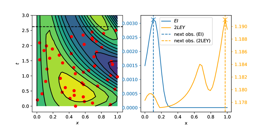
(a) Left: contour of $f(\mathbf{x},t)$ in $\bm{\mathcal{X}}\times\mathcal{T}$ with $T=3$. Red circles denote the locations of $n$ previous observations. Horizontal line denotes the time $t_{n+1}=2.625$ at which the next observation is to be made. Right: myopic (EI) and lookahead (2LEY) acquisition functions.

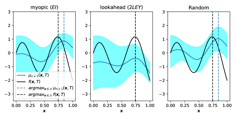
(b) GP prediction at $T$ with decisions incorporated from myopic (EI) and lookahead (2LEY) decisions as well as a decision chosen uniformly at random from $\boldsymbol{\mathcal{X}}$ at $t$. Shaded region represents 95% confidence region.

Figure 1: Comparison of the decisions made via a myopic (EI) and a lookahead (2LEY) acquisition function. The top right shows the acquisition functions and the respective decisions (maximizers). The GP predictions, incorporating the decision made via either of the acquisition functions, are shown in the bottom. One can see that if the final decision at $T$ is made as $\operatornamewithlimits{arg\,max}_{\mathbf{x}\in\bm{\mathcal{X}}}~{}\mu_{n+1}(\mathbf{x},T)$, then the lookahead approach predicts the maximizer at $T$ more accurately than does the myopic approach. A random decision $(0.2474,2.625)$, even though it is space filling, does not outperform the lookahead decision.

In foundational work on lookahead BO, Osborne [24] showed that proper Bayesian reasoning can be used to define an acquisition function where the ($n+1$)th observation is made by marginalizing a loss function at the final ($q$th) observation over all the remaining observations $(\mathbf{x}_{i},\hat{y}_{i})$, $i=n+2,\ldots,q$. Others have proposed lookahead EI in the context of finite-budget BO. For example, Ginsbourger and Le Riche [10] showed that the lookahead EI is a dynamic program that chooses the EI maximizer in expectation, considering all possible strategies of the same budget. A practical challenge with lookahead strategies is the computational tractability (as demonstrated in, for example, [10, 24]), which can be partially mitigated by various approximation methods [11, 19, 40]. Yue and Kontar [41] explored the theoretical properties of the approximate dynamic programming approach for multistep lookahead acquisition functions and discussed when these strategies are guaranteed to perform better than their myopic counterparts. In this work we draw inspiration from [24] to address the limited budget aspect of our problem. However, we propose a general framework for lookahead BO that readily applies to the finite-horizon, time-dependent BO; we are unaware of any previous work on this topic.

In the context of time-dependent BO, the only works we are aware of are [23] and [2]. We fundamentally differ from their approach in the following ways: (i) their goal is to track a time-varying optimum whereas ours is to predict it at the target horizon $T$), and (ii) they do not address the limited budget constraint as we do. Furthermore, setting $k_{t}(t_{i},t_{j})=(1-\epsilon)^{|t_{i}-t_{j}|/2}$ (where $\epsilon$ is the forgetting factor as defined in [2]), our method is equivalent to [2] if we myopically make decisions at each $t$ via UCB.

Another plausible way to solve the finite-horizon (target $t=T$) BO problem is to sequentially choose points that are most informative [7] about the maximizer at the target horizon; see, for example, [13, 14, 36]. Although such information-theoretic approaches are known to involve an intractable form of the information entropies, they are also highly reliant on an accurate underlying GP model [20].

In this work, we extend myopic acquisition functions in order to make nonmyopic decisions for finite-horizon BO. Specifically, we propose a generalized framework that specifies a value function that quantifies an objective at the target horizon $T$ and that can then be used in a lookahead acquisition function. Our main contributions are as follows.

1. We present the first strategy to solve finite-horizon BO for time-dependent oracles.

2. We propose lookahead versions of myopic acquisition functions (section 2) that are applicable to both finite-budget BO and finite-horizon, time-dependent settings.

3. We present a practical algorithm that recursively applies a two-step lookahead acquisition function (section 3) to make new observations time-dependent oracles.

4. We establish the utility of our method by demonstrating it on carefully constructed synthetic test functions (sections 5.1 and 5.2) and a real-world quantum optimal control problem (section 5.3).

Software that implements our lookahead framework for limited horizon, finite-budget time-dependent BO problems is available upon request and will be released publicly with the final version of this manuscript.

The remainder of the paper is organized as follows. In section 2 we present our generalized lookahead acquisition framework for generic value functions. In section 3 we present a recursive two-step lookahead approach that is more practical than a more-than-two-step lookahead approach. We discuss theoretical properties of our approach in section 4. We then present the results of our numerical experiments on synthetic test functions (sections 5.1 and 5.2) as well as a real-world quantum optimal control problem in section 5.3. We conclude the paper with an outlook on future work.

2 Generalized m-step lookahead acquisition function

Given the data from $n$ observations $\bm{\mathcal{D}}_{n}$, let us define a value function $\upsilon$ by

$$\upsilon_{n}(\mathbf{x},t;\boldsymbol{\omega}):=\mathbb{E}_{y\sim Y|\bm{\mathcal{D}}_{n}}\left[h(y(\mathbf{x},t);\boldsymbol{\omega})\right],$$ (4)

where $h$ is a scalar-valued function, $\boldsymbol{\omega}\in\mathbb{R}^{p}$ are parameters that parameterize $h$, $Y|\bm{\mathcal{D}}_{n}$ is the GP posterior given $n$ observations, and $y(\mathbf{x},t)$ is a sample path realized from $Y(\mathbf{x},t)$. For example, the PI, EI, and UCB acquisition functions can be obtained from defining $h$ as

$$\begin{split}h(y(\mathbf{x},t);\xi)&=y(\mathbf{x},t)-\xi\implies\upsilon(\mathbf{x},t;\xi)=\Phi\left(z\right)\qquad\text{(PI)}\\ h(y(\mathbf{x},t);\xi)&=[y(\mathbf{x},t)-\xi]^{+}\implies\upsilon(\mathbf{x},t;\xi)=z\sigma(\mathbf{x},t)\Phi\left(z\right)+\sigma_{n}(\mathbf{x},t)\phi\left(z\right)\qquad\text{(EI)}\\ h(y(\mathbf{x},t);\beta)&=y(\mathbf{x},t)+\beta^{1/2}\sigma(\mathbf{x},t)\implies\upsilon(\mathbf{x},t;\beta)=\mu(\mathbf{x},t)+\beta^{1/2}\sigma(\mathbf{x},t),\qquad\text{(UCB)}\end{split}$$ (5)

where recall that $\xi$ and $\beta$ are user-specified target and confidence parameters, respectively. Similarly, when $h$ is the identity function $h(y(\mathbf{x},t);\boldsymbol{\omega})=y(\mathbf{x},t)$, then $\upsilon(\mathbf{x},t)=\mu(\mathbf{x},t)$.

We use the following notation for conciseness:

$$\mathbf{x}^{t}_{n+1}:=(\mathbf{x},t_{n+1}) \bm{\mathcal{D}}_{n,j}:=\bm{\mathcal{D}}_{n}\bigcup_{i=1,\ldots,j}\{\mathbf{x}^{t}_{n+i},y_{n+i}\}$$

$$y_{n+1}:=y(\mathbf{x}^{t}_{n+1}) \mathbb{E}_{n,j}:=\mathbb{E}_{y\sim Y|\bm{\mathcal{D}}_{n,j}}$$

$$\mu_{n,j}:=\mathbb{E}_{n,j}Y,~{}~{}\sigma^{2}_{n,j}:=\mathbb{E}_{n,j}\left(Y-\mu_{n,j}\right)^{2} \upsilon^{T}_{n,j}:=\upsilon_{n,j}(\mathbf{x},T;\boldsymbol{\omega})=\mathbb{E}_{n,j}~{}\left[h(y(\mathbf{x},T);\boldsymbol{\omega})\right],$$

where we note that whenever we explicitly use $y(\mathbf{x},t)$, we refer to a sample path drawn from $Y(\mathbf{x},t)$ and therefore $y_{n+1}=y(\mathbf{x}_{n+1},t_{n+1})$ is a draw from $y(\mathbf{x},t)$ at $(\mathbf{x}_{n+1},t_{n+1})$. On the other hand, when we use $\hat{y}_{i}$, we refer to an observation of the oracle at $(\mathbf{x}_{i},t_{i})$. Similarly, note that $\bm{\mathcal{D}}_{n,k}$ contains $n$ oracle evaluations and $k$ candidate points $\mathbf{x}$ and the $k$ corresponding draws from the GP at times $t_{n+1}$, …, $t_{n+k}$. Furthermore, we note here that $\mathbf{x}^{t}_{n+1}$ is $d$-dimensional.

We define our $m$-step lookahead acquisition function as

$$\begin{split}\alpha_{m}(\mathbf{x}^{t}_{n+1})=\int\ldots\int&\left[\max_{\tilde{\mathbf{x}}\in\bm{\mathcal{X}}}~{}\upsilon_{n,m-1}(\tilde{\mathbf{x}},T;\boldsymbol{\omega})|\bm{\mathcal{D}}_{n,m-1}\right]~{}p(y_{n+m-2}|\bm{\mathcal{D}}_{n,m-2})\\ &p(\mathbf{x}^{t}_{n+m-1}|\bm{\mathcal{D}}_{n,m-2})\cdots p(y_{n}|\bm{\mathcal{D}}_{n})~{}dy_{n+m-2}\cdots dy_{n}~{}d\mathbf{x}^{t}_{n,m-1}\cdots d\mathbf{x}^{t}_{n+2}.\end{split}$$ (6)

Note that in (6), the inner maximization is always with respect to $\mathbf{x}$ at $t=T$ and that after evaluating the integral, the resulting expression is a function of $\mathbf{x}^{t}_{n+1}$. Furthermore, since we are interested in choosing the maximizer of $\alpha_{m}(\mathbf{x}^{t}_{n+1})$ for $t_{n+1}$, we do not marginalize $\mathbf{x}^{t}_{n+1}$. Computing (6) involves the computation of $m-1$ nested expectations. Additionally, when the expectations are approximated via Monte Carlo sampling, there is a total of $N\times(m-1)$ $d$-dimensional optimization solves due to the inner maximization in (6). The computation or even the Monte Carlo approximation of (6) becomes intractable as $m$ increases, warranting further approximation, as is done, for instance, in [11, 19, 41]. When $m=2$, however, the computation of (6) is much more straightforward, as we discuss in the following section.

3 Generalized two-step lookahead acquisition function

In this work, as a practical alternative to the computationally intractable multistep ($m>2$) lookahead acquisition function, we recursively optimize the two-step lookahead acquisition function (8) at each time step of the time-dependent BO problem; this process is graphically described in fig. 2. Given $\bm{\mathcal{D}}_{n}$ and with $m=2$, we define our two-step lookahead acquisition function by

$$\begin{array}[]{rl}\alpha_{2}(\mathbf{x},t_{n+1})\par&=\displaystyle\int\max_{\tilde{\mathbf{x}}\in\bm{\mathcal{X}}}~{}\left[\upsilon_{n,1}(\tilde{\mathbf{x}},T;\boldsymbol{\omega})|\,\bm{\mathcal{D}}_{n}\bigcup\{(\mathbf{x},t_{n+1}),y_{n+1}\}\right]~{}p(y_{n}|\bm{\mathcal{D}}_{n})~{}dy_{n},\end{array}$$ (7)

where $p(y_{n}|\bm{\mathcal{D}}_{n})$ is the probability density of the GP posterior distribution conditioned on $\bm{\mathcal{D}}_{n}$. We write (7) concisely as

$$\alpha_{2}(\mathbf{x}^{t}_{n+1})=\mathbb{E}_{n}\left[\max_{\tilde{\mathbf{x}}\in\bm{\mathcal{X}}}~{}\upsilon_{n,1}(\tilde{\mathbf{x}},T;\boldsymbol{\omega})|\bm{\mathcal{D}}_{n,1}\right].$$ (8)

In (8), recall that $\bm{\mathcal{D}}_{n,1}$ is the union of $\bm{\mathcal{D}}_{n}$ and the $n+1$th observation being a draw from the GP $Y_{n}$, and we compute $\upsilon_{n,1}(\tilde{\mathbf{x}},T;\boldsymbol{\omega})$ by taking the expectation with respect to $Y|\bm{\mathcal{D}}_{n,1}$. In general, it is not guaranteed that (8) admits a closed-form expression. Hence we make the Monte Carlo approximation

$$\alpha_{2}(\mathbf{x}^{t}_{n+1})\approx\hat{\alpha}_{2}(\mathbf{x}^{t}_{n+1}):=\frac{1}{N}\sum_{j=1}^{N}\max_{\tilde{\mathbf{x}}\in\bm{\mathcal{X}}}~{}\upsilon_{n,1}^{T,j},$$ (9)

where $\upsilon_{n,1}^{T,j}=\upsilon_{n,1}(\tilde{\mathbf{x}},T)|y^{j}_{n+1}$ with the $N$ iid samples $\{y^{j}_{n+1}:\,j=1,\ldots,N\}$ drawn from $Y_{n}$. In practice, the computation of (8) involves the following steps (given $\mathbf{x}_{n+1}$):

1. Generate $N$ iid samples $\{y^{j}_{n+1}\}_{i=1}^{N}$ drawing from $\mathcal{N}(\mu_{n}(\mathbf{x}_{n+1},t_{n+1}),\sigma_{n}^{2}(\mathbf{x}_{n+1},t_{n+1}))$.

2. For each $y^{j}_{n+1},~{}j=1,\ldots,N$

   1. update $\bm{\mathcal{D}}_{n}$ to $\bm{\mathcal{D}}_{n,1}$ to get GP posterior $Y|\bm{\mathcal{D}}_{n,1}$ and

   2. maximize a draw of the projected value function $\nu^{j}=\max_{\tilde{\mathbf{x}}\in\bm{\mathcal{X}}}~{}\upsilon_{n,1}(\tilde{\mathbf{x}},T)|\bm{\mathcal{D}}_{n,1}$.

3. Compute $\hat{\alpha}_{2}(\mathbf{x}_{n+1})\approx\frac{1}{N}\sum_{j=1}^{N}\nu^{j}$.

In order to make a decision at $t_{n+1}$, (8) needs to be maximized. We show how the maximization of the acquisition function can be done efficiently by constructing unbiased estimators of the acquisition function’s gradient. Under suitable regularity conditions, we can interchange the expectation and gradient operators (see theorem 4.2 ) to obtain

$$\nabla_{\mathbf{x}}\alpha_{2}(\mathbf{x}^{t}_{n+1})=\mathbb{E}_{n}\left[\nabla_{\mathbf{x}}~{}\max_{\tilde{\mathbf{x}}\in\bm{\mathcal{X}}}~{}\upsilon_{n,1}(\tilde{\mathbf{x}},T)|\bm{\mathcal{D}}_{n,1}\right].$$ (10)

Similar to the Monte Carlo approximation for the acquisition function presented in (9), (10) can be approximated as

$$\nabla_{\mathbf{x}}\alpha_{2}(\mathbf{x}^{t}_{n+1})\approx\tilde{\nabla}_{\mathbf{x}}\alpha_{2}(\mathbf{x}^{t}_{n+1})=\frac{1}{N}\sum_{i=1}^{N}d\nu^{i}:=\frac{1}{N}\sum_{i=1}^{N}\nabla_{\mathbf{x}}~{}\max_{\tilde{\mathbf{x}}\in\bm{\mathcal{X}}}~{}\upsilon_{n,1}^{T,i}.$$ (11)

In this way, sample-averaged gradients can be used in a gradient-based optimizer to efficiently optimize (8). We clarify the issues associated with computing the gradients of functions involving the $\max()$ operator as in (11) in Section 4.

We now illustrate in detail the two-step acquisition function for a specific value function.

Two-step lookahead expected oracle value (2LEY) acquisition function

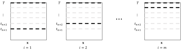
Figure 2: Recursive two-step lookahead method for time-dependent problems. Here, we start with $n$ observations up to $t_{n}$ and have $q-n$ remaining observations to make, where $q$ is the total budget. We sequentially select one point $\mathbf{x}_{n+i}$ at each step that maximizes the expected value function evaluated at $T$; this is denoted by the black dashed lines at $t_{n+i}$ and $T$, whereas the gray dashed lines denote the remaining decisions to be made. We repeat the same process until the decision is made at the penultimate step $i=q-1$. The final decision at $T$ is made by maximizing the value function at $T$.

As an illustration, we set $h$ to be the identity function, and hence $\upsilon_{n,1}(\mathbf{x},T)=\mu_{n,1}(\mathbf{x},T)|\bm{\mathcal{D}}_{n,1}$. We define our two-step lookahead expected oracle value (2LEY) acquisition function as

$$\begin{split}\alpha_{2LEY}(\mathbf{x}^{t}_{n+1}):=&\mathbb{E}_{n}\left[\underset{\tilde{\mathbf{x}}\in\bm{\mathcal{X}}}{\max}~{}\left.\mu_{n,1}(\tilde{\mathbf{x}},T)\right|\bm{\mathcal{D}}_{n,1}\right]\\ =&\mathbb{E}_{n}\left[\mu^{*}_{n,1}(\mathbf{x}^{t}_{n+1},T)\right],\end{split}$$ (12)

where $\mu^{*}_{n,1}=\mu_{n,1}(\mathbf{x}^{*},T)$ with $\mathbf{x}^{*}$ being a maximizer of $\mu_{n,1}(\mathbf{x},T)|\bm{\mathcal{D}}_{n,1}$ and $y_{n+1}$ is a draw from $\mathcal{N}\left(\mu_{n}(\mathbf{x}^{t}_{n+1}),\sigma_{n}^{2}(\mathbf{x}^{t}_{n+1})\right)$. The dependence of the second line of (12) on $\mathbf{x}^{t}_{n+1}$ can be seen by realizing that

$$\mu_{n,1}^{*}(\mathbf{x}^{t}_{n+1},T)=\mathbf{k}_{n+1}^{\top}\mathbf{K}^{-1}_{n+1}[\mathbf{y}_{n}^{\top},y_{n+1}]^{\top},$$ (13)

where $\mathbf{k}_{n+1}=[k\left((\mathbf{x}^{*},T),(\mathbf{x}_{1},t_{1})\right),\ldots,k\left((\mathbf{x}^{*},T),(\mathbf{x}_{n},t_{n})\right),k\left((\mathbf{x}^{*},T),(\mathbf{x}_{n+1},t_{n+1})\right)]^{\top}$, and $\mathbf{K}_{n+1,ij}=k\left((\mathbf{x}_{i},t_{i}),(\mathbf{x}_{j},t_{j})\right);~{}\forall i=1,\ldots,n+1,~{}j=1,\ldots,n+1$. The expectation in (12) is approximated as

$$\alpha_{2LEY}(\mathbf{x}^{t}_{n+1})=\mathbb{E}_{n}\left[\mu_{n,1}^{*}(\mathbf{x}^{t}_{n+1},T)\right]\approx\frac{1}{N}\sum_{j=1}^{N}\mu_{n,1}^{*}(\mathbf{x}^{t}_{n+1},T)|y^{j}_{n+1}.$$ (14)

The gradient of $\mu_{n,1}^{*}(\mathbf{x}^{t}_{n+1},T)$ with respect to $\mathbf{x}^{t}_{n+1}$ is given by

$$\begin{split}\nabla_{\mathbf{x}}\mu_{n,1}^{*}(\mathbf{x}^{t}_{n+1},T)=&\frac{\partial\mathbf{k}_{n+1}^{\top}}{\partial\mathbf{x}_{n+1}}\mathbf{K}^{-1}_{n+1}+\mathbf{k}_{n+1}^{\top}\frac{\partial\mathbf{K}^{-1}_{n+1}}{\partial\mathbf{x}_{n+1}}\\ =&\frac{\partial\mathbf{k}_{n+1}^{\top}}{\partial\mathbf{x}_{n+1}}\mathbf{K}^{-1}_{n+1}+\mathbf{k}_{n+1}^{\top}~{}\mathbf{K}^{-1}_{n+1}\frac{\partial\mathbf{K}_{n+1}}{\partial\mathbf{x}_{n+1}}\mathbf{K}^{-1}_{n+1},\end{split}$$ (15)

where $\frac{\partial\mathbf{K}_{n+1}}{\partial\mathbf{x}_{n+1}}$ is a matrix of elementwise derivatives and the second line follows from a well-known lemma on the derivative of a matrix inverse [26, pp. 201–202].

With a continuously differentiable kernel $k(\cdot,\cdot)$, we have that

$$\nabla_{\mathbf{x}}\alpha_{2LEY}(\mathbf{x}^{t}_{n+1})=\nabla_{\mathbf{x}}\mathbb{E}_{n}\left[\mu_{n,1}^{*}(\mathbf{x}^{t}_{n+1},T)\right]=\mathbb{E}_{n}\left[\nabla_{\mathbf{x}}\mu_{n,1}^{*}(\mathbf{x}^{t}_{n+1},T)\right],$$ (16)

where the interchange of the gradient and expectation operators is via theorem 4.2. Then the gradient is approximated as

$$\nabla_{\mathbf{x}}\alpha_{2LEY}(\mathbf{x}^{t}_{n+1})=\mathbb{E}_{n}\left[\nabla_{\mathbf{x}}\mu_{n,1}^{*}(\mathbf{x}^{t}_{n+1},T)\right]\approx\frac{1}{N}\sum_{j=1}^{N}\nabla_{\mathbf{x}}\mu_{n,1}^{*}(\mathbf{x}^{t}_{n+1},T)|y^{j}_{n+1}.$$ (17)

Furthermore, (14) and (17) are unbiased estimators for $\alpha_{2LEY}$ and $\nabla_{\mathbf{x}}\alpha_{2LEY}$, respectively; see theorem 4.2. This gradient can then be used in a gradient-based optimizer to maximize our two-step lookahead acquisition function in an efficient manner.

Similarly, the two-step lookahead extensions for EI, PI, and UCB are obtained by picking the corresponding value functions as $\alpha_{\textrm{EI}}(\mathbf{x},T)$, $\alpha_{\textrm{PI}}(\mathbf{x},T)$ and $\alpha_{\textrm{UCB}}(\mathbf{x},T)$ and are named respectively, $\alpha_{2LEI}$, $\alpha_{2LPI}$, and $\alpha_{2LUCB}$. Our overall algorithm recursively maximizes the two-step acquisition function until the penultimate step and maximizes the actual value function at the final step. The overall algorithm is graphically depicted in fig. 2 and is presented in Algorithm 2. We refer to Algorithm 2 with the value functions chosen as $\mu_{n,1}(\mathbf{x},T)$, $\alpha_{EI}$, $\alpha_{PI}$, and $\alpha_{UCB}$ as r2LEY, r2LEI, r2LPI, and r2LUCB, respectively.

1 Given: $\bm{\mathcal{D}}_{n}$, total budget $q$, schedule $\{t_{n+1},\ldots,t_{q}:=T\}$, and GP hyperparameters $\bm{\Omega}$

Result: $(\mathbf{x}_{T},\hat{y}_{T})$

2 for $i=n+1,\ldots,q-1$,  do

3       Define value function $\upsilon^{T}_{i-1,1}|\bm{\mathcal{D}}_{i-1,1}$

4       Find $\mathbf{x}_{i}=\underset{\mathbf{x}\in\bm{\mathcal{X}}}{\operatornamewithlimits{arg\,max}}~{}\hat{\alpha}_{2}(\mathbf{x},t_{i})$,   (acquisition function maximization)

5        with $\hat{\alpha}_{2}$ and $\nabla_{\mathbf{x}}~{}\hat{\alpha}_{2}$ evaluated via (9) and (11) resp.

6       Observe $\hat{y}_{i}$ = $f(\mathbf{x}_{i},t_{i})+\epsilon_{i}$

7       Append $\bm{\mathcal{D}}_{i}=\bm{\mathcal{D}}_{i-1}\cup\{(\mathbf{x}_{i},t_{i}),\hat{y}_{i}\}$

8       Update GP hyperparameters $\bm{\Omega}$

9      

10 end for

11Find $\mathbf{x}_{T}\in\underset{\mathbf{x}\in\bm{\mathcal{X}}}{\operatornamewithlimits{arg\,max}}~{}\upsilon_{q}(\mathbf{x},T)|\bm{\mathcal{D}}_{q-1}$   (value function maximization)

12 Observe $\hat{y}_{T}$ = $f(\mathbf{x}_{T},T)+\epsilon_{T}$

Algorithm 2 Recursive two-step lookahead Bayesian optimization

4 Theoretical properties

We now present the theoretical foundation of our method and a few properties. Let $\mathcal{Y}$ be the support of $y_{n+1}$, whose density is $p(y_{n+1})$. As before, let the domain of $\mathbf{x}^{t}_{n+1}$ be $\bm{\mathcal{X}}$.

We make the following remark about the differentiability of our acquisition function; this justifies the interchange of the gradient and expectation operators.

Remark 4.1

We write the inner term of our two-step lookahead acquisition function in (8) as $\max_{\mathbf{x}\in\bm{\mathcal{X}}}\mathbb{E}_{n,1}h(y)$, where we omit the arguments of $y$ and $\boldsymbol{\omega}$ for the sake of conciseness. The GP posterior mean $\mu(\mathbf{x},t)$ and standard deviation $\sigma(\mathbf{x},t)$ are continuously differentiable with the sufficient condition that we choose a continuously differentiable prior covariance kernel $k$ [29, 35]. We then use the reparameterization trick [38, 37] to write the GP sample path as $y(\mathbf{x},T):=\mu(\mathbf{x},T)+\sigma(\mathbf{x},T)\times\gamma$, where $\gamma\sim\mathcal{N}(0,1)$, which makes the differentiability of our acquisition function transparent.

From a purely implementation standpoint, we use the gradient $\nabla\max_{\tilde{\mathbf{x}}\in\bm{\mathcal{X}}}{\mathbb{E}_{n,1}~{}h(y)}$ if it exists and a subgradient [3] otherwise. In our implementation, the gradients are computed by backpropagating the output of the $\max()$ operation; in Appendix A we provide examples of how (sub)gradients are calculated for nonsmooth functions.

Let $\mathbf{x}^{*}$ be a maximizer of $\mathbb{E}_{n,1}h(y(\mathbf{x},T);\boldsymbol{\omega})=\upsilon_{n,1}(\mathbf{x},T)|\bm{\mathcal{D}}_{n,1}$. In what follows, we write $g^{*}(\mathbf{x}^{t}_{n+1},T,y_{n+1}):=\upsilon_{n,1}(\mathbf{x}^{*},T)|\bm{\mathcal{D}}_{n,1}$ to denote the maximum value of the value function at $T$ after having updated $\bm{\mathcal{D}}_{n}$ with $y_{n+1}$, and $\nabla_{\mathbf{x}}g^{*}:=\partial g^{*}(\mathbf{x}^{t}_{n+1},T,y_{n+1})/\partial\mathbf{x}^{t}_{n+1}$. Note again that the dependence of $g^{*}$ on $\mathbf{x}^{t}_{n+1}$ is due to $\bm{\mathcal{D}}_{n,1}$.

Theorem 4.2 (Interchange of gradient and expectation operators)

Let $\nabla_{\mathbf{x}}g^{*}$ exist, and let $g^{*}(\mathbf{x}^{t}_{n+1},T,y_{n+1})\times p(y_{n+1})$ and $\nabla_{\mathbf{x}}g^{*}\times p(y_{n+1})$ be continuous on $\bm{\mathcal{X}}\times\mathcal{Y}$. Further assume that there exist functions $q_{0}$ and $q_{1}$ such that

$$\begin{array}[]{rl}|g^{*}(\mathbf{x}^{t}_{n+1},T,y_{n+1})\times p(y_{n+1})|&\leq q_{0}(y_{n+1})\\ \|\nabla_{\mathbf{x}}g^{*}\times p(y_{n+1})\|&\leq q_{1}(y_{n+1})\end{array}\qquad\forall(\mathbf{x}^{t}_{n+1},y_{n+1})\in\bm{\mathcal{X}}\times\mathcal{Y},$$

where $\int_{\mathcal{Y}}q_{1}(y_{n+1})dy_{n+1}<\infty$ and $\int_{\mathcal{Y}}q_{2}(y_{n+1})dy_{n+1}<\infty$. Then,

$$\nabla_{\mathbf{x}}\mathbb{E}_{j}\left[g^{*}(\mathbf{x}^{t}_{n+1},T,y_{n+1})\right]=\mathbb{E}_{n}\left[\nabla_{\mathbf{x}}g^{*}(\mathbf{x}^{t}_{n+1},T,y_{n+1})\right].$$

Furthermore, a realization of $\nabla_{\mathbf{x}}g^{*}(\mathbf{x}^{t}_{n+1},T,y_{n+1})$ yields an unbiased estimate of the gradient of $\alpha_{2}(\mathbf{x}_{n+1}^{t})$ in (8).

Proof: Using $g^{*}(\mathbf{x}^{t}_{n+1})$ to denote $g^{*}(\mathbf{x}^{t}_{n+1},T,y_{n+1})$ for the sake of brevity, we have

$$\begin{split}\nabla_{\mathbf{x}}\alpha_{2}(\mathbf{x}^{t}_{n+1}):=\frac{\partial}{\partial\mathbf{x}^{t}_{n+1}}\mathbb{E}_{n}\left[g^{*}(\mathbf{x}^{t}_{n+1})\right]&=\underset{h\rightarrow 0}{\textnormal{lim}}~{}\frac{1}{h}\left\{\mathbb{E}_{n}\left[g^{*}(\mathbf{x}^{t}_{n+1}+h)\right]-\mathbb{E}_{n}\left[g^{*}(\mathbf{x}^{t}_{n+1})\right]\right\}\\ &=\underset{h\rightarrow 0}{\textnormal{lim}}~{}\left\{\mathbb{E}_{n}\frac{1}{h}\left[g^{*}(\mathbf{x}^{t}_{n+1}+h)-g^{*}(\mathbf{x}^{t}_{n+1})\right]\right\}\\ &=\underset{h\rightarrow 0}{\textnormal{lim}}~{}\left\{\mathbb{E}_{n}\frac{\partial g^{*}(\bar{\mathbf{x}}^{h}_{n+1})}{\partial\mathbf{x}_{n+1}}\right\},\\ \end{split}$$ (18)

where $\bar{\mathbf{x}}^{h}_{n+1}=\lambda\mathbf{x}^{t}_{n+1}+(1-\lambda)(\mathbf{x}^{t}_{n+1}+h)$ for some $\lambda\in[0,1]$ and the last line follows from the first-order mean value theorem. We bring the limit inside the integral by Lebesgue’s dominated convergence theorem to obtain

$$\frac{\partial}{\partial\mathbf{x}^{t}_{n+1}}\mathbb{E}_{n}\left[g^{*}(\mathbf{x}^{t}_{n+1})\right]=\mathbb{E}_{n}~{}\underset{h\rightarrow 0}{\textnormal{lim}}\frac{\partial g^{*}(\bar{\mathbf{x}}^{h}_{n+1})}{\partial\mathbf{x}^{t}_{n+1}}=\mathbb{E}_{n}\frac{\partial g^{*}(\mathbf{x}^{t}_{n+1})}{\partial\mathbf{x}^{t}_{n+1}}.$$ (19)

Since (18) holds, a realization $\partial g^{*}(\mathbf{x}^{t}_{n+1})/\partial\mathbf{x}^{t}_{n+1}$ yields an unbiased estimate of the gradient $\nabla_{\mathbf{x}}\alpha_{2}(\mathbf{x}^{t}_{n+1})$.  

Proposition 4.3 (Special case when $m=2$ and $\upsilon^{T}=\mu(\mathbf{x},T)$)

When $m=2$, our 2LEY acquisition function is equivalent to the knowledge gradient (KG) [8, 39] acquisition function offset by a constant factor.

Proof: The KG acquisition function, in the context of our problem, is given as

$$\alpha_{KG}(\mathbf{x}^{t}_{n+1})=\mathbb{E}_{n}\left[\underset{\tilde{\mathbf{x}}\in\bm{\mathcal{X}}}{\max}~{}\mu_{n,1}(\tilde{\mathbf{x}},T)|\bm{\mathcal{D}}_{n,1}\right]-\underset{\mathbf{x}\in\bm{\mathcal{X}}}{\max}~{}\mu_{n}(\mathbf{x},T).$$ (20)

With $m=2$, the 2LEY acquisition function at $\mathbf{x}_{n+1}$ is defined as follows:

$$\begin{split}\alpha_{2LEY}(\mathbf{x}^{t}_{n+1})&=\int_{y_{n}}\left[\max_{\tilde{\mathbf{x}}\in\bm{\mathcal{X}}}~{}\mathbb{E}_{n,1}~{}y(\tilde{\mathbf{x}},T)|\bm{\mathcal{D}}_{n,1}\right]p(y_{n}|\bm{\mathcal{D}}_{n})~{}dy_{n}\\ &=\int_{y_{n}}\left[\max_{\tilde{\mathbf{x}}\in\bm{\mathcal{X}}}~{}\mu_{n,1}(\tilde{\mathbf{x}},T)|\bm{\mathcal{D}}_{n,1}\right]p(y_{n}|\bm{\mathcal{D}}_{n})~{}dy_{n}\\ &=\mathbb{E}_{n}\left[\max_{\tilde{\mathbf{x}}\in\bm{\mathcal{X}}}~{}\mu_{n,1}(\tilde{\mathbf{x}},T)|\bm{\mathcal{D}}_{n,1}\right]\\ &=\alpha_{KG}(\mathbf{x}^{t}_{n+1})+\max_{\tilde{\mathbf{x}}\in\bm{\mathcal{X}}}~{}\mu_{n}(\tilde{\mathbf{x}},T),\end{split}$$ (21)

where the last line follows from eq. 20. Note that $\alpha_{2LEY}$ and $\alpha_{KG}$ share the same maximizer.  

Proposition 4.4 (Special case when $|T-t|\gg\theta_{t}$)

With the prior assumption $f(\mathbf{x},t)\sim\mathcal{GP}(0,k(\cdot,\cdot))$, where $k(\cdot,\cdot):=k_{\mathbf{x}}(\cdot,\cdot;~{}\theta_{\mathbf{x}})\times k_{t}(\cdot,\cdot;~{}\theta_{t})$, with $k_{\mathbf{x}}$ and $k_{t}$ being squared-exponential kernels, our two-step lookahead acquisition function approaches $\alpha_{2}(\mathbf{x}^{t}_{n+1})=\max_{\tilde{\mathbf{x}}\in\bm{\mathcal{X}}}{\upsilon_{n}(\tilde{\mathbf{x}},T)}$ as $|T-t_{n+1}|\rightarrow\infty$. In other words, far away from the target horizon $T$, $\alpha_{2}(\mathbf{x}^{t}_{n+1})$ approaches a constant function.

Proof: When $|T-t_{n+1}|\gg\theta_{t}$, then $k_{t}(t_{n+1},T)\approx 0$; this yields $k\left((\mathbf{x},t_{n+1}),(\mathbf{x},T)\right)\approx 0$. Let $\mu_{n}$ and $\sigma_{n}^{2}$ be the posterior mean and variance given $\bm{\mathcal{D}}_{n}$, respectively. Given another observation $y_{n+1}$ drawn from the GP $Y_{n}$ at $(\mathbf{x},t_{n+1})$, where $|T-t_{n+1}|\gg\theta_{t}$, the updated posterior mean and variance are given by

$$\begin{split}\mu_{n,1}=&\mathbf{k}^{\top}_{n+1}\mathbf{K}^{-1}_{n+1}[\mathbf{y}^{\top}_{n},y_{n+1}]^{\top}\approx[\mathbf{k}^{\top}_{n},0]\begin{bmatrix}\mathbf{K}_{n}&\mathbf{0}\\ \mathbf{0}&1\end{bmatrix}^{-1}[\mathbf{y}^{\top}_{n},y_{n+1}]^{\top}=\mu_{n}\\ \sigma^{2}_{n,1}=&1-\mathbf{k}^{\top}_{n+1}\mathbf{K}^{-1}_{n+1}\mathbf{k}_{n+1}\approx 1-[\mathbf{k}^{\top}_{n},0]\begin{bmatrix}\mathbf{K}_{n}&\mathbf{0}\\ \mathbf{0}&1\end{bmatrix}^{-1}[\mathbf{k}^{\top}_{n},0]^{\top}=\sigma_{n}^{2},\end{split}$$ (22)

where we have assumed, without loss of generality, that $k((\mathbf{x},t),(\mathbf{x},t))=1$ and have used the matrix inversion lemma. Therefore, writing our acquisition function using the reparameterization trick, we see that

$$\begin{split}\alpha_{2}(\mathbf{x}^{t}_{n+1})=&\mathbb{E}_{n}\left[\max_{\tilde{\mathbf{x}}\in\bm{\mathcal{X}}}{\mathbb{E}_{n,1}~{}h(y(\tilde{\mathbf{x}},T))}\right]\\ =&\mathbb{E}_{n}\left[\max_{\tilde{\mathbf{x}}\in\bm{\mathcal{X}}}{\mathbb{E}_{\gamma}~{}h(\mu_{n,1}(\tilde{\mathbf{x}},T)+\sigma_{n,1}(\tilde{\mathbf{x}},T)\gamma)}\right]\\ \approx&\mathbb{E}_{n}\left[\max_{\tilde{\mathbf{x}}\in\bm{\mathcal{X}}}{\mathbb{E}_{\gamma}~{}h(\mu_{n}(\tilde{\mathbf{x}},T)+\sigma_{n}(\tilde{\mathbf{x}},T)\gamma)}\right]\\ =&\max_{\tilde{\mathbf{x}}\in\bm{\mathcal{X}}}{\upsilon_{n}(\tilde{\mathbf{x}},T)},\end{split}$$ (23)

and thus, in the limit $|T-t_{n+1}|\rightarrow\infty$, $\alpha_{2}(\mathbf{x}^{t}_{n+1})=\max_{\tilde{\mathbf{x}}\in\bm{\mathcal{X}}}{\upsilon_{n}(\tilde{\mathbf{x}},T)}$.  

Remark 4.5

Following Proposition 4.4, one can see that if $k_{t}(t_{n+1},T)\approx 0$, then $k_{t}(t_{i},T)\approx 0,~{}\forall i=1,\ldots,n$ since $t_{i}>t_{i-1}$. This further leads to $\mathbf{k}_{n+1}\approx\mathbf{0}$ and hence $\mu_{n,1}\approx 0$ and $\sigma_{n,1}^{2}\approx 1$. This results in (for $|T-t_{n+1}|\gg\theta_{t}$),

$$\begin{split}\alpha_{2}(\mathbf{x}^{t}_{n+1})=&\mathbb{E}_{n}\left[\max_{\tilde{\mathbf{x}}\in\bm{\mathcal{X}}}{\mathbb{E}_{\gamma}~{}h(\mu_{n}(\tilde{\mathbf{x}},T)+\sigma_{n}(\tilde{\mathbf{x}},T)\gamma)}\right]\\ \approx&\mathbb{E}_{n}\left[\max_{\tilde{\mathbf{x}}\in\bm{\mathcal{X}}}{\mathbb{E}_{\gamma}~{}h(\gamma)}\right]\\ =&c,\end{split}$$ (24)

where $c$ is some constant. Suppose the $(n+1)$th decision is made by maximizing $\alpha_{2}(\mathbf{x}^{t}_{n+1})$ with a multistart local optimization procedure started from a set of starting points $\{\mathbf{x}\}\in\bm{\mathcal{X}}$, where $\{\mathbf{x}\}$ are sampled from distribution $p_{\mathbf{x}}$. Then, in the limit $|T-t_{n+1}|\rightarrow\infty$, decisions made via our lookahead acquisition function are equivalent to samples drawn randomly from $p_{\mathbf{x}}$.

We take advantage of this property and set $p_{\mathbf{x}}=\mathcal{U}(\bm{\mathcal{X}})$, where $\mathcal{U}$ is the uniform distribution. In practice, this could result in a decisions that explore $\bm{\mathcal{X}}$ when the $T$ is far away and hence can lead to improved learning of $f(\mathbf{x},t)$, thus facilitating a more accurate prediction of the maximum at $T$.

5 Numerical experiments

We demonstrate our proposed approach on synthetic test cases and a quantum optimal control problem.

We compare our method with widely used myopic approaches in BO, namely, EI, PI, and UCB. We refer to “EImumax” and “PImumax” as the EI and PI strategies, respectively, with the target $\xi$ set as the maximum of the GP posterior mean at the current step, that is, $\underset{\mathbf{x}\in\bm{\mathcal{X}}}{\max}~{}\mu(\mathbf{x},t)$. We set the confidence parameter for UCB to $\beta=2$. Additionally, we compare our method with “mumax,” which selects points by maximizing the GP posterior mean at the current time. We also make direct comparisons between the myopic acquisition functions and their lookahead counterparts. Moreover, we compare our method with a strategy that selects points uniformly at random from $\mathbf{x}\sim\mathcal{U}(\bm{\mathcal{X}})$; we call this acquisition function “Random.”

Our metric for comparison is the oracle value $f(\mathbf{x}_{T},T)$ at the target time $T$. Each query to $f(\mathbf{x},t)$ includes additive noise with mean zero and variance $\sigma_{\epsilon}^{2}=10^{-3}$. Each repetition of each experiment is provided with starting samples that include oracle evaluations at a set of points distributed with uniform spacing in $[0,t_{\textnormal{start}}]$ with each point sampled uniformly at random in $\bm{\mathcal{X}}$, where $t_{\textnormal{start}}<T$ is arbitrarily set for each experiment. Within each repetition the same starting samples are given to all acquisition functions.

5.1 Synthetic one-dimensional test cases

Our synthetic test functions take the form $f(\mathbf{x},t)=f_{\mathbf{x}}(\mathbf{x})+f_{\mathbf{x}t}(\mathbf{x},t)$ or $f(\mathbf{x},t)=f_{\textnormal{ref}}(\mathbf{x}(t))$ in order to induce time dependence to the maximizer of $f(\mathbf{x},t)$.

We first consider quadratic one-dimensional functions $f_{\mathbf{x}}$ over the domain $\bm{\mathcal{X}}=[0,1]$ with

$$f_{\mathbf{x}}(\mathbf{x})=-4(\mathbf{x}-0.5)^{2}.$$ (25)

The time-dependent component takes the following four forms:

$$\begin{split}\textnormal{Quadratic-a}:\quad f_{\mathbf{x}t}=&\sin\left(\pi(\mathbf{x}+t)\right)+\cos\left(\pi(\mathbf{x}+t)\right)\\ \textnormal{Quadratic-b}:\quad f_{\mathbf{x}t}=&\sin\left(\pi(\mathbf{x}t)\right)+\textnormal{cos}\left(\pi(\mathbf{x}t)\right)\\ \textnormal{Quadratic-c}:\quad f_{\mathbf{x}t}=&\sin\left(\pi(\mathbf{x}[t-3]^{+})\right)+\textnormal{cos}\left(\pi(\mathbf{x}[t-3]^{+})\right)\\ \textnormal{Quadratic-d}:\quad f_{\mathbf{x}t}=&2\mathbf{x}\textnormal{sin}(t)-\textnormal{sin}^{2}(t),\end{split}$$

where $[t-3]^{+}\equiv\max(0,t-3)$ is specified to induce movement of $\mathbf{x}_{t}^{*}$ for $t\geq 3$. fig. 3 shows the trajectories of $\mathbf{x}_{t}^{*}$, the maximizer at time $t$, for each of these test cases.

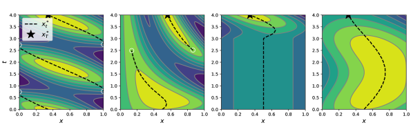
Figure 3: One-dimensional synthetic test cases. The dashed line represents the trajectory of $\mathbf{x}_{t}^{*}$.

These test cases are deliberately designed to reflect a variety of situations, such as discontinuous change of $\mathbf{x}^{*}_{t}$ (Quadratic-a and Quadratic-b) and sudden dynamics (Quadratic-c).

fig. 4 compares the points selected by our lookahead approach with various value functions and the corresponding myopic approaches. In each plot 20 repetitions are overlaid, with samples in $\bm{\mathcal{X}}\times[0,1]$ used to start all of the methods; white circles denote the points chosen by each method at times $t>1$. The lookahead BO does not try to track a moving maximizer, which results in points being more spread out in a space-filling fashion than with myopic acquisition functions. This approach is particularly beneficial in handling oracles whose maximizers can go through a discontinuous change (e.g., Quadratic-a and Quadratic-b). In the case of Quadratic-c, we demonstrate (see further details in fig. 5(b)) that our algorithm is able to handle oracles where $\mathbf{x}_{t}^{*}$ may undergo sudden dynamics ($\approx t=3.0$ in this case). For Quadratic-d, where the challenges of the other one-dimensional cases do not exist, the algorithm performs much better in predicting $\mathbf{x}_{T}^{*}$.

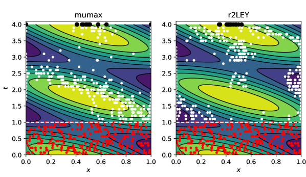
(a) Quadratic-a

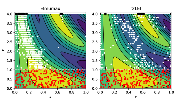
(b) Quadratic-b

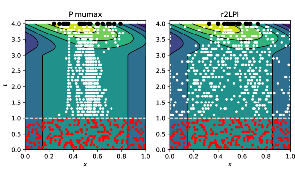
(c) Quadratic-c

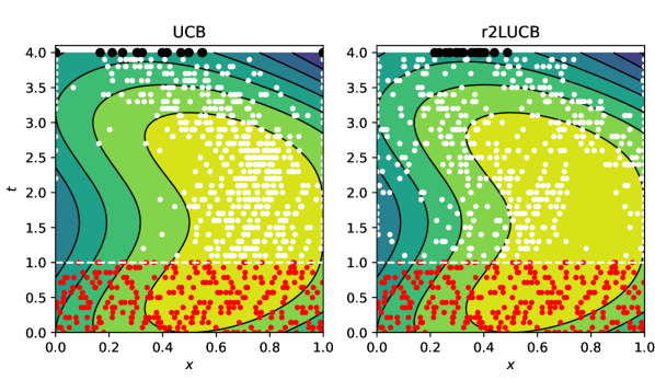
(d) Quadratic-d

Figure 4: Comparison of our two-step lookahead (right) and myopic (left) acquisition functions on the one-dimensional synthetic test cases. The plot shows an overlay of 20 repetitions of the algorithm with (shared) random starting points. The white circles denote the decision made at each step, and the contours in the background represents the true noise-free oracle $f(\mathbf{x},t)$

fig. 5 compares the time history of the average oracle value (over 20 replications with randomized starting points) resulting from decisions made via the myopic and lookahead acquisition functions. We present results for only Quadratic-a and Quadratic-c for the sake of brevity. One can see that the lookahead acquisition functions (dashed line plots) make decisions with lower oracle value during the early rounds. While the acquisition function per se does not seek to make decisions with low current oracle value, the consequence of looking ahead at $T$ is that decisions made at current $t$ may incur a low oracle value. This is a fundamental distinction between our proposed lookahead and the myopic acquisition functions. Also, the average oracle value at target time $T$ (denoted by the empty circle) is consistently higher than the myopic counterparts (denoted by the square). Furthermore, the predictions by the lookahead acquisition functions are with higher confidence, as visualized by the error bars (one standard deviation in the predictions) shown at $T$; note that we highlight the error bars for the lookahead acquisition functions in black.

The average oracle values at $T$ predicted by all the acquisition functions are somewhat consistent, with the r2LEY being one of the most competitive, including the rest of the test cases. For this reason, moving forward we predominately use the r2LEY as the representative lookahead acquisition function.

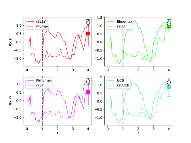
(a) Quadratic-a

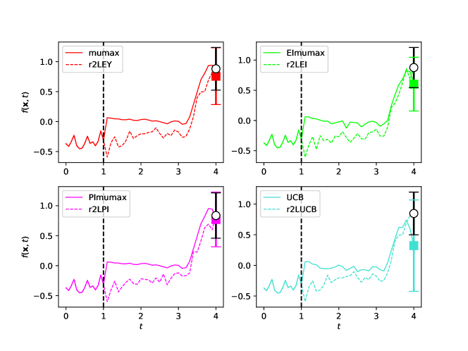
(b) Quadratic-c

Figure 5: Average of 20 replications with random starting points of the myopic (lookahead) acquisition function on one-dimensional test cases. The final point at $T=4$ is highlighted with square (circle) symbols and variability at $T$ is visualized via colored (black) error bars. The vertical dashed line represents the time until which $n=15$ starting points are collected and the total budget is set to $q=45$.

5.2 Synthetic higher dimensional test cases

We now demonstrate our method on higher-dimensional test functions, up to $d=6$. We begin by presenting a modified Griewank function ($d=2$) [32], where we multiply the original Griewank function $f_{\textnormal{ref}}$ by a Gaussian weight function in order to create a unique global maximum. Then, we modify the input $\mathbf{x}\in\bm{\mathcal{X}}=[-5,5]^{2}$ with a time-dependent rotation to yield the function

$$f(\mathbf{x},t)=f_{\textnormal{ref}}(\mathbf{x}(t))\times\textnormal{exp}~{}\left(-\|\mathbf{x}-\mathbf{x}_{0}\|^{2}/\ell\right),$$ (26)

where $\mathbf{x}_{0}=[3,0]$, $\ell\in\mathbb{R}_{+}$ is a scaling constant and $\mathbf{x}(t)=R(\zeta_{t})\times\mathbf{x},$ where

$$R(\zeta_{t})=\begin{bmatrix}\cos(\zeta_{t})&-\sin(\zeta_{t})\\ \sin(\zeta_{t})&\cos(\zeta_{t})\end{bmatrix}$$

is a $2\times 2$ rotation matrix and $\zeta_{t}=\pi t/4$. Time snapshots of this test function are shown in fig. 6 and illustrate a counterclockwise rotation of the unique global maximizer with time. As before, all oracle observations include additive mean zero noise with variance $\sigma_{\epsilon}^{2}=10^{-3}$.

The performance of all the myopic acquisition functions is compared against r2LEY in fig. 7, where the contour plot at $T$ is shown with the predictions from 20 repetitions of each acquisition function (black $\times$ symbols) overlaid. Note that the total budget is fixed at $q=90$, where $n=60$ is used in $\bm{\mathcal{X}}\times[2,3]$ to start the algorithm, and the target time is $T=4$. The lookahead acquisition function clearly predicts the global maximum at $T$ with greater consistency than the rest do; all but two repetitions predicted $\mathbf{x}_{T}$ such that $\|\mathbf{x}_{T}-\mathbf{x}^{*}_{T}\|<0.26$.

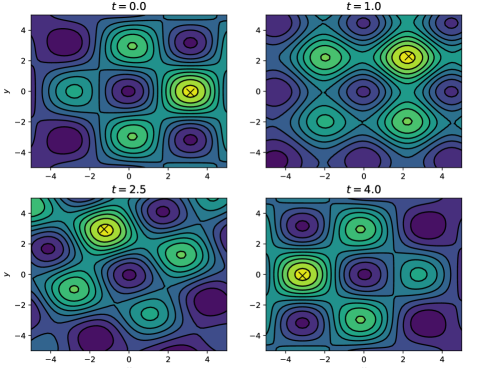
Figure 6: Time snapshots of the modified Griewank function. Notice the unique global maximum at each time and the counterclockwise rotation of the global maximizer with time.

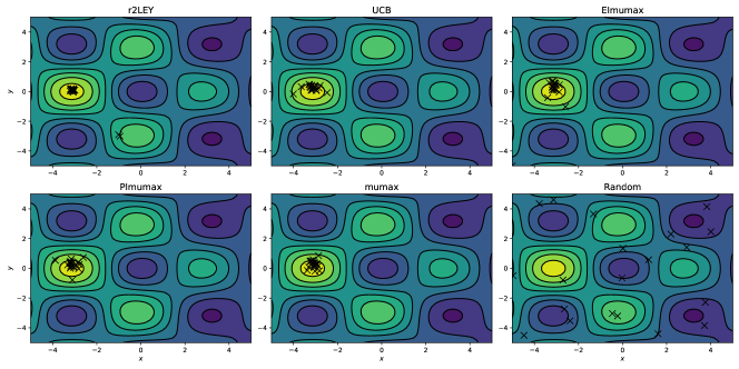
Figure 7: Predictions at $T=4.0$ on the modified Griewank test case. Symbols represent predictions at $T$ after 20 repetitions of each algorithm, and the contours represent the noise-free $f(\mathbf{x},T)$. The total budget is set to $q=90$, where $n=60$ samples in $2.0\leq t\leq 3.0$ are used to start each algorithm.

We also demonstrate our method on the Hartmann-3d ($d=3$) and Hartmann-6d ($d=6$) test functions. In both cases, the Hartmann function [32] is summed with $f_{\mathbf{x}t}(\mathbf{x},t)=\mathbf{1}^{\top}[2\textnormal{sin}(t)\mathbf{x}-\textnormal{sin}^{2}(t)\mathbf{1}]$ (where $\mathbf{1}$ is a vector of ones of length $d$) to induce movement of the maximum with time. For Hartmann-3d, the total budget is set to $q=120$ with $n=90$ samples queried in $[0,1]^{3}\times[2,3]$ to start the algorithm. For Hartmann-6d, we set $q=150$ with $n=120$ samples queried in $[0,1]^{3}\times[2,3]$ to start the algorithm, and our target time is $T=4$. Figure 8 shows the time histories of $f(\mathbf{x}_{i},t)$ averaged over 20 replications. The predictions at $T$ are highlighted by adding a marker in the plot. In both test functions, the lookahead acquisition function results in a higher oracle value $f(\mathbf{x}_{T},T)$ at the target time $T$ compared with other myopic acquisition functions.

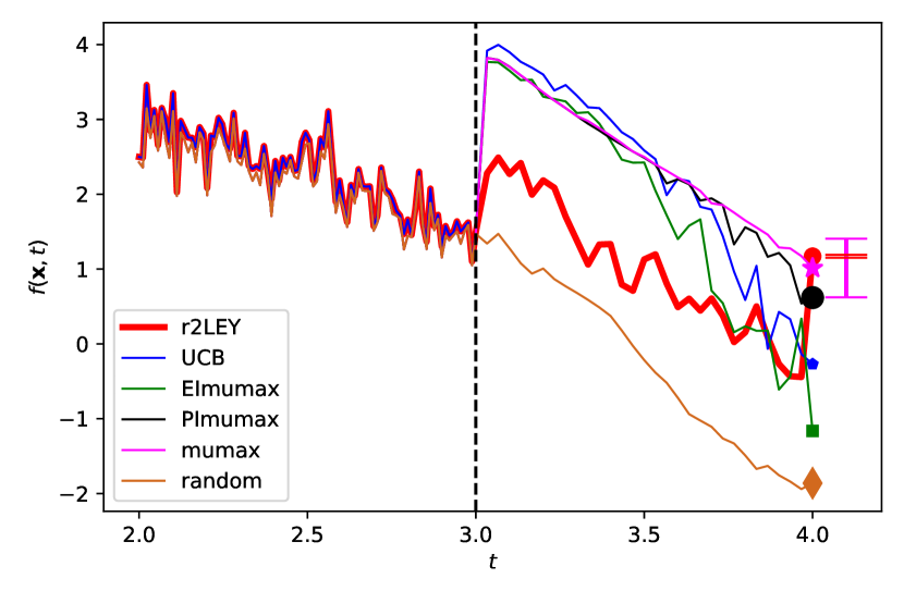
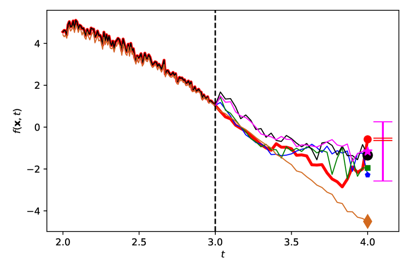
Figure 8: Hartmann-3d ($d=3$) and Hartmann-6d ($d=6$) test functions. Average of 20 repetitions. Left of vertical line corresponds to starting samples. The error bars for the oracle value at $T$ for the best two acquisition functions (r2LEY and mumax) shown are slightly shifted in time for better visibility. The r2LEY shows comparatively less variability.

5.3 Quantum optimal control

We next compare methods for optimizing time-dependent oracles on a challenging real-world problem. Optimally shaping electromagnetic fields to control quantum systems is a widespread application [4]; similar problems appear when controlling molecular transformations relevant to chemical, biological, and materials science applications. Quantum optimal control (QOC) is a method to shape electromagnetic fields to steer a quantum system toward a desired control target; see fig. 9 where the target is a specific outcome from a chemical reaction.

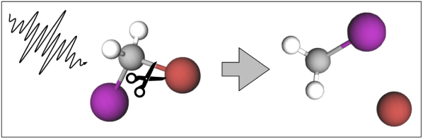
Figure 9: Illustration of QOC to control chemical reactions. A femtosecond laser controlled by QOC is used to provide control over the selective dissociation of molecules. Figure source: [21]

The problem we consider is based on a diatomic molecule HF, whose vibrational energy mode is modeled as a nonrotating Morse oscillator on a 1D grid that varies with time and is illuminated with a laser field to induce dissociation. The electromagnetic field is parameterized by a set of coefficients $\mathbf{x}\in\bm{\mathcal{X}}\subset\mathbb{R}^{5}$ that are the control parameters; more specifically, $\mathbf{x}$ contains the frequency components of the electromagnetic field. The digital quantum simulation of the Morse oscillator $f(\mathbf{x},t)$ takes as input the control parameter $\mathbf{x}$ and a terminal time $t\in[0,T]$—which is not to be confused with our target time $T$—whose output is the observable control objective that needs to be minimized with respect to $\mathbf{x}$. The cost of each query of the simulation increases monotonically with the terminal time $t$, and we are interested in finding the optimal control at a specific target time $T$. Since searching for the optimal control at $T$ is expensive, we seek to predict the optimal control at $T$ with cheaper evaluations of $f(\mathbf{x},t)$ for $t<T$.

In this regard, we use BO to find the control parameters $\mathbf{x}_{T}^{*}$ that maximize the negative value of $f(\mathbf{x},T),\forall\mathbf{x}\in\bm{\mathcal{X}}$. We begin by collecting observations of their system $\bm{\mathcal{D}}_{n}=\{(\mathbf{x}_{i},t_{i}),\hat{y}_{i}\},~{}i=1,\ldots,n$, which we use to fit a GP that emulates $f$ in $\bm{\mathcal{X}}\times{\mathcal{T}}$. Then, we sequentially make observations $\{(\mathbf{x}_{i},t_{i}),\hat{y}_{i}\},~{}i=n+1,\ldots,q$, where each $\mathbf{x}_{i}$ is selected by maximizing our proposed two-step lookahead acquisition function. Figure 10 provides a schematic of this problem. To conform to our problem setting, we allow evaluations only at increasing values of $t$. See [21] for more information about this problem.

We set the total budget to $q=180$, where $n=150$ samples are queried over $4000\leq t\leq 5000$ to start the algorithm and $T=6000$. The time histories of each acquisition function for the QOC problem are shown in fig. 11, where we include results from r2LEY and r2LPI among the lookahead approaches. The best-known maximum $f(\mathbf{x}^{*},T)=0.0$ at $T=6000$, which is shown in the figure as the black square. In terms of the average performance, the lookahead r2LEY outperforms all other methods, with the mumax being a close competitor, as shown in the top-left of Figure 11. We visualize the variability in the predictions at $T$ via boxplots in the top right of Figure 11, where we observe that the r2LEY has the highest median oracle value to interquartile distance ratio. This shows that although r2LEY does not result in the best median oracle value, it provides the most confident prediction, while still being competitive with UCB and mumax. Even though the lookahead method r2LPI does not necessarily outperform all the other myopic methods, it shows better performance—in terms of both average and median oracle value—compared with its myopic counterpart PImumax. This behavior is consistent with what was observed with the one-dimensional test cases presented in section 5.1.

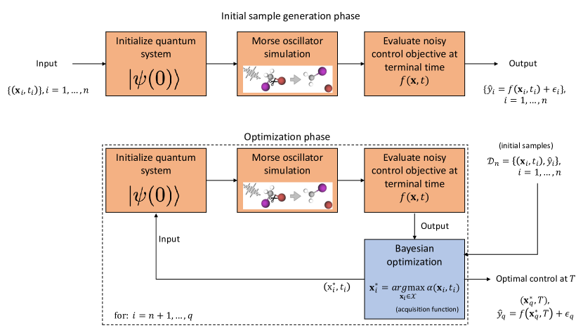
Figure 10: Overview of the quantum optimal control problem recreated from [21]. The quantum system dynamics, driven by a field parameterized by $\mathbf{x}$, are simulated for the time range $[0,t]$ (where $t$ is the terminal time), after which the control objective function $f(\mathbf{x},t)$ is calculated. A recent framework [21] is proposed for efficiently evaluating the control objective function by using a future quantum computer. During an initial sample generation phase, the control objective function is evaluated $n$ times to generate initial samples $\bm{\mathcal{D}}_{n}$ that are used by the GP to learn $f(\mathbf{x},t),~{}\mathbf{x}\in\bm{\mathcal{X}},t\in[0,t]$. Then, in the optimization phase, the trained GP is used in the BO framework to find the optimal control at target time $T$. The inputs at $(\mathbf{x}_{i},t_{i}),~{}i=,n+1,\ldots,q$ are chosen at optimal locations as guided by the BO acquisition function optimization.

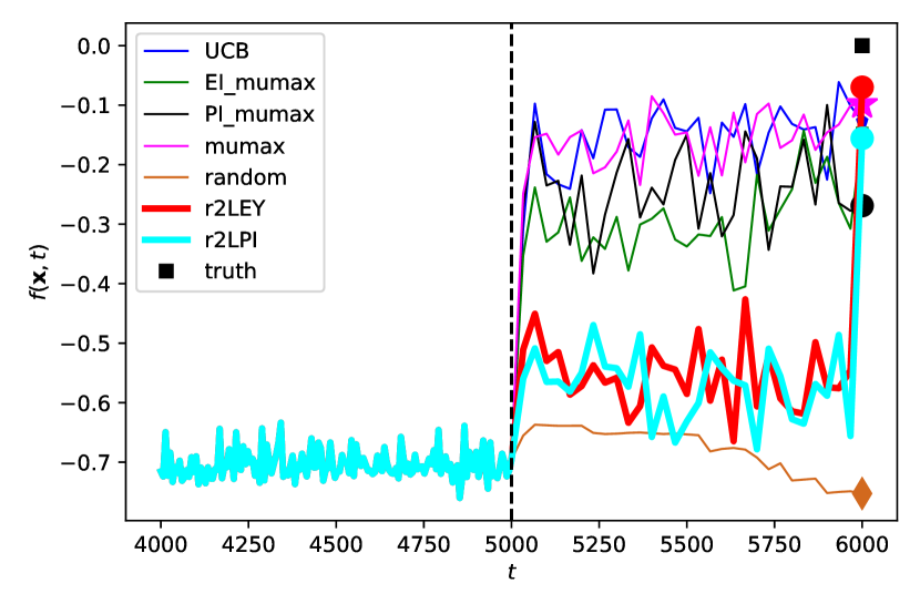
(a) Average $f(\mathbf{x},t)$ over 20 repetitions with randomized starting points. Left of vertical line denotes starting points.

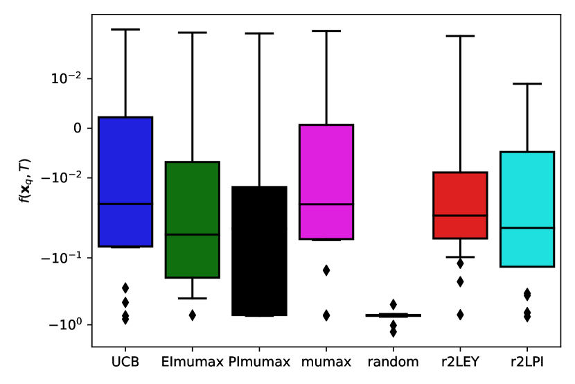
(b) Variability in the oracle value at $T$, $f(\mathbf{x},T)$.

Figure 11: Demonstration on the quantum optimal control problem.

5.4 Implementation details

We implemented our recursive lookahead Bayesian optimization framework in PyTorch [25] using the GP and BO libraries GPyTorch [9] and BoTorch, respectively [1]. For finite-horizon time-dependent BO with limited budget, the lookahead acquisition functions outperform their myopic counterparts in securing the best oracle value at the horizon. This improved accuracy comes at the cost of additional computational overhead in terms of optimizing the acquisition functions. Our Monte Carlo approximation to the acquisition function and its gradients, as presented in Line 5 of Algorithm 2, lends itself well to be used with a gradient-based optimizer. For further computational improvements, however, we also adopt the one-shot optimization of the lookahead acquisition function as implemented in BoTorch. The approach formulates line 4 of Algorithm 2 as a deterministic optimization problem over the joint $\mathbf{x}$ and $\mathbf{x}^{\prime}$, where $\mathbf{x}^{\prime}:=\{\mathbf{x}^{j}\}_{j=1}^{N}$ are the candidate maximizers or fantasy points. While this increases the dimensionality of the optimization problem from $d$ to $N+d$, we observe consistent results (with our Monte Carlo approach) with $N$ set to as small as 32, resulting in significant computational speedup. Moreover, the one-shot approach solves a deterministic optimization problem as opposed to a stochastic optimization problem with the Monte Carlo approach. We include both the Monte Carlo and one-shot approaches in our software and recommend the latter as the dimensionality $d$ of the problem increases; all the results presented in this work are based on the one-shot approach. For the $d=5$ QOC problem, the acquisition function optimization takes approximately 30 seconds of wall-clock time when run in serial. Because many of the time-dependent oracles we are targeting require significantly more computational cost and time, we consider the per-iterate cost of our approach to be trivial. Furthermore, the PyTorch framework allows for leveraging advanced computation hardware such as graphics processing units, which may allow for further computational efficiency.

6 Conclusions and future work

Bayesian optimization with a lookahead acquisition function outperforms well-known myopic acquisition functions in solving the finite-budget, finite-horizon, time-dependent maximization of an expensive stochastic oracle. Specifically, for such problems, the lookahead approach makes probabilistically sound decisions that give better average-case returns at the target horizon, while considering strategies that lead up to the target horizon. In this regard, the lookahead acquisition functions take advantage of the epistemic uncertainty—explained by the GP—in the predictions about the oracle. In this work we introduce a generalized framework that offers lookahead extensions to widely known myopic acquisition functions. We demonstrate our method on illustrative synthetic test functions (that involve discontinuities in the oracle maximizer) as well as a quantum optimal control application problem. Because of the lack of analytically closed-form expressions for our lookahead acquisition functions, their construction (and optimization) incurs more computational overhead than do the myopic acquisition functions. Such an overhead is insignificant, however, when optimizing expensive stochastic oracles that take, for example, hours of wall-clock time per evaluation. Overall, we demonstrate that our proposed acquisition function results in more confident and accurate predictions of the global maxima at the target horizon compared with Bayesian optimization using myopic acquisition functions.

The primary challenge with handling time-dependent optimization problems with BO is that the effect of the dynamics of the oracle has to be learned by a GP model. When the distance to the horizon is large, it is particularly challenging to train a global GP that emulates the oracle in $\bm{\mathcal{X}}\times\mathcal{T}$. A natural alternative is to work with local GPs within local regions that are dynamically updated. This is one avenue for future work that we are considering.

A related problem is multifidelity BO (see, e.g., [30, 16, 33]) in which one seeks to solve $\max_{\mathbf{x}\in\bm{\mathcal{X}}}~{}f(\mathbf{x})$ using observations of $\hat{f}(\mathbf{x},s)$. The fidelity is given by the parameter $s\in[0,1]$, with $f(\mathbf{x}):=\hat{f}(\mathbf{x},1)$ corresponding to the highest fidelity. Typically, there is a cost function $c(s)\in\mathbb{R}$, which is monotonically increasing in the fidelity level $s$. By placing a GP prior on the function $\hat{f}(\mathbf{x},s)$ directly, one can sequentially optimize acquisition functions such as

$$\max_{(\mathbf{x},s)\in\bm{\mathcal{X}}\times[0,1]}~{}\frac{\alpha(\mathbf{x},s)}{c(s)}.$$

Our problem is equivalent to the multifidelity BO problem with $s$ replaced by $t\in[0,T]$ with the following key differences:

1. In our case, $\hat{f}(\mathbf{x},T)$ can never be observed when $t<T$. More generally, any set $\{t_{i}\},i=1,\ldots,n$ has a unique ordering $t_{1}<\ldots<t_{n}$; and while we are at any $t_{i}$, evaluation of $f(\mathbf{x},t\neq t_{i})$ is not possible.

2. We make only one observation $f(\mathbf{x},t)$ for each $t\in[0,T]$.

3. The cost of each evaluation $c(s)=c$ is a constant. However, similar to the general multifidelity framework, we are still interested in maximizing $f(\mathbf{x},T)$.

Another area of future work is defining a time-dependent cost function that can be used within the multifidelity framework to also select the time schedule of observations automatically; this approach is of specific interest in handling continuous-time systems.

Appendix A Gradient computation with PyTorch

We show two examples of nondifferentiable functions in Figure 12: (i) $f(\mathbf{x})=\sin(|\mathbf{x}|)$ and (ii) $f(\mathbf{x})=\max(\mathbf{x},\mathbf{x}^{2})$. In (i) the nondifferentiability occurs at $\mathbf{x}=0$, and in (ii) the nondifferentiability occurs at both $\mathbf{x}=0$ and $\mathbf{x}=1.0$, where the subgradient returned by PyTorch is shown in the figure.

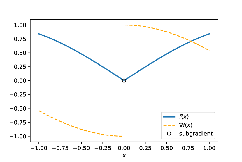
(a) $f(\mathbf{x})=\sin(|\mathbf{x}|)$

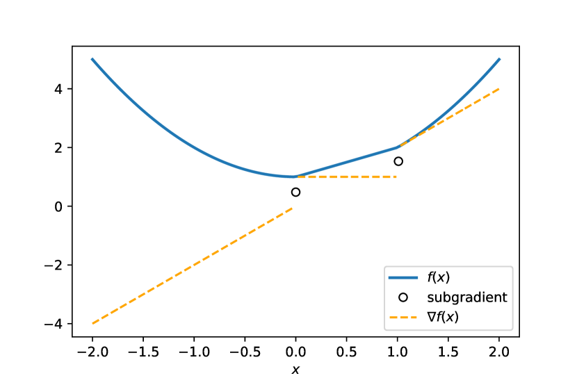
(b) $f(\mathbf{x})=\max(\mathbf{x},\mathbf{x}^{2})$

Figure 12: Examples of nondifferentiable functions and their (sub)gradients. At points of nondifferentiability, we indicate the subgradient returned by PyTorch.

References

- [1] M. Balandat, B. Karrer, D. R. Jiang, S. Daulton, B. Letham, A. G. Wilson, and E. Bakshy, BoTorch: Programmable Bayesian optimization in PyTorch, arXiv:1910.06403, (2019).
- [2] I. Bogunovic, J. Scarlett, and V. Cevher, Time-varying Gaussian process bandit optimization, in Proceedings of the 19th International Conference on Artificial Intelligence and Statistics, 2016, pp. 314–323.
- [3] S. Boyd, S. P. Boyd, and L. Vandenberghe, Convex Optimization, Cambridge University Press, 2004.
- [4] C. Brif, R. Chakrabarti, and H. Rabitz, Control of quantum phenomena: past, present and future, New Journal of Physics, 12 (2010), p. 075008.
- [5] E. Brochu, V. M. Cora, and N. De Freitas, A tutorial on Bayesian optimization of expensive cost functions, with application to active user modeling and hierarchical reinforcement learning, arXiv:1012.2599, (2010).
- [6] A. D. Bull, Convergence rates of efficient global optimization algorithms, Journal of Machine Learning Research, 12 (2011), pp. 2879–2904.
- [7] T. M. Cover and J. A. Thomas, Elements of Information Theory, John Wiley & Sons, 2012, https://doi.org/10.1002/047174882X.
- [8] P. I. Frazier, W. B. Powell, and S. Dayanik, A knowledge-gradient policy for sequential information collection, SIAM Journal on Control and Optimization, 47 (2008), pp. 2410–2439, https://doi.org/10.1137/070693424.
- [9] J. Gardner, G. Pleiss, K. Q. Weinberger, D. Bindel, and A. G. Wilson, GPyTorch: Blackbox matrix-matrix Gaussian process inference with GPU acceleration, in Advances in Neural Information Processing Systems, 2018, pp. 7576–7586.
- [10] D. Ginsbourger and R. Le Riche, Towards Gaussian process-based optimization with finite time horizon, in Contributions to Statistics, Springer, 2010, pp. 89–96, https://doi.org/10.1007/978-3-7908-2410-0_12.
- [11] J. Gonzalez, M. Osborne, and N. Lawrence, GLASSES: Relieving the myopia of Bayesian optimisation, in Proceedings of the 19th International Conference on Artificial Intelligence and Statistics, A. Gretton and C. C. Robert, eds., vol. 51 of Proceedings of Machine Learning Research, 2016, pp. 790–799, http://proceedings.mlr.press/v51/gonzalez16b.html.
- [12] R. B. Gramacy, Surrogates: Gaussian Process Modeling, Design and Optimization for the Applied Sciences, Chapman Hall/CRC, Boca Raton, Florida, 2020, http://bobby.gramacy.com/surrogates.
- [13] P. Hennig and C. J. Schuler, Entropy search for information-efficient global optimization, Journal of Machine Learning Research, 13 (2012), pp. 1809–1837.
- [14] J. M. Hernández-Lobato, M. W. Hoffman, and Z. Ghahramani, Predictive entropy search for efficient global optimization of black-box functions, in Advances in Neural Information Processing Systems, 2014, pp. 918–926.
- [15] D. R. Jones, M. Schonlau, and W. J. Welch, Efficient global optimization of expensive black-box functions, Journal of Global Optimization, 13 (1998), pp. 455–492, https://doi.org/10.1023/A:1008306431147.
- [16] K. Kandasamy, G. Dasarathy, J. Schneider, and B. Póczos, Multi-fidelity Bayesian optimisation with continuous approximations, arXiv:1703.06240, (2017).
- [17] A. Krause and C. S. Ong, Contextual Gaussian process bandit optimization, in Advances in Neural Information Processing Systems, 2011, pp. 2447–2455.
- [18] H. J. Kushner, A new method of locating the maximum point of an arbitrary multipeak curve in the presence of noise, Journal of Basic Engineering, 86 (1964), pp. 97–106, https://doi.org/10.1115/1.3653121.
- [19] R. Lam, K. Willcox, and D. H. Wolpert, Bayesian optimization with a finite budget: An approximate dynamic programming approach, in Advances in Neural Information Processing Systems, 2016, pp. 883–891.
- [20] D. J. MacKay, Information-based objective functions for active data selection, Neural Computation, 4 (1992), pp. 590–604, https://doi.org/10.1162/neco.1992.4.4.590.
- [21] A. B. Magann, M. D. Grace, H. A. Rabitz, and M. Sarovar, Digital quantum simulation of molecular dynamics and control, arXiv:2002.12497, (2020).
- [22] J. Mockus, V. Tiešis, and A. Žilinskas, The application of Bayesian methods for seeking the extremum, Towards Global Optimization, 2 (1978), pp. 117–129.
- [23] F. M. Nyikosa, M. A. Osborne, and S. J. Roberts, Bayesian optimization for dynamic problems, arXiv.org/1803.03432, (2018).
- [24] M. A. Osborne, Bayesian Gaussian Processes for Sequential Prediction, Optimisation and Quadrature, PhD thesis, Oxford University, UK, 2010.
- [25] A. Paszke, S. Gross, F. Massa, A. Lerer, J. Bradbury, G. Chanan, T. Killeen, Z. Lin, N. Gimelshein, L. Antiga, A. Desmaison, A. Kopf, E. Yang, Z. DeVito, M. Raison, A. Tejani, S. Chilamkurthy, B. Steiner, L. Fang, J. Bai, and S. Chintala, PyTorch: An imperative style, high-performance deep learning library, in Advances in Neural Information Processing Systems 32, H. Wallach, H. Larochelle, A. Beygelzimer, F. d'Alché-Buc, E. Fox, and R. Garnett, eds., Curran Associates, Inc., 2019, pp. 8024–8035, http://papers.neurips.cc/paper/9015-pytorch-an-imperative-style-high-performance-deep-learning-library.pdf.
- [26] C. E. Rasmussen and C. K. I. Williams, Gaussian Processes for Machine Learning, MIT Press, 2006, https://doi.org/10.7551/mitpress/3206.001.0001.
- [27] B. Shahriari, K. Swersky, Z. Wang, R. P. Adams, and N. De Freitas, Taking the human out of the loop: A review of Bayesian optimization, Proceedings of the IEEE, 104 (2015), pp. 148–175, https://doi.org/10.1109/jproc.2015.2494218.
- [28] A. Shapiro, D. Dentcheva, and A. Ruszczyński, Lectures on Stochastic Programming: Modeling and Theory, SIAM, 2014, https://doi.org/10.1137/1.9780898718751.
- [29] S. P. Smith, Differentiation of the Cholesky algorithm, Journal of Computational and Graphical Statistics, 4 (1995), pp. 134–147, https://doi.org/10.2307/1390762.
- [30] J. Song, Y. Chen, and Y. Yue, A general framework for multi-fidelity Bayesian optimization with Gaussian processes, in The 22nd International Conference on Artificial Intelligence and Statistics, PMLR, 2019, pp. 3158–3167.
- [31] N. Srinivas, A. Krause, S. M. Kakade, and M. Seeger, Gaussian process optimization in the bandit setting: No regret and experimental design, in Proceedings of the International Conference on Machine Learning, 2009.
- [32] S. Surjanovic and D. Bingham, Virtual library of simulation experiments: Test functions and datasets. Retrieved May 23, 2020, from http://www.sfu.ca/~ssurjano.
- [33] S. Takeno, H. Fukuoka, Y. Tsukada, T. Koyama, M. Shiga, I. Takeuchi, and M. Karasuyama, Multi-fidelity Bayesian optimization with max-value entropy search, arXiv:1901.08275, (2019).
- [34] E. Vazquez and J. Bect, Convergence properties of the expected improvement algorithm with fixed mean and covariance functions, Journal of Statistical Planning and Inference, 140 (2010), pp. 3088–3095, https://doi.org/10.1016/j.jspi.2010.04.018.
- [35] J. Wang, S. C. Clark, E. Liu, and P. I. Frazier, Parallel Bayesian global optimization of expensive functions, arXiv:1602.05149, (2016).
- [36] Z. Wang and S. Jegelka, Max-value entropy search for efficient Bayesian optimization, in Proceedings of the 34th International Conference on Machine Learning, vol. 70, 2017, pp. 3627–3635.
- [37] J. T. Wilson, F. Hutter, and M. P. Deisenroth, Maximizing acquisition functions for Bayesian optimization, arXiv:1805.10196, (2018).
- [38] J. T. Wilson, R. Moriconi, F. Hutter, and M. P. Deisenroth, The reparameterization trick for acquisition functions, arXiv:1712.00424, (2017).
- [39] J. Wu and P. Frazier, The parallel knowledge gradient method for batch Bayesian optimization, in Advances in Neural Information Processing Systems, 2016, pp. 3126–3134.
- [40] J. Wu and P. Frazier, Practical two-step lookahead Bayesian optimization, in Advances in Neural Information Processing Systems, 2019, pp. 9810–9820.
- [41] X. Yue and R. A. Kontar, Why non-myopic Bayesian optimization is promising and how far should we look-ahead? A study via rollout, in International Conference on Artificial Intelligence and Statistics, PMLR, 2020, pp. 2808–2818.
- [42] D. Zhu, N. M. Linke, M. Benedetti, K. A. Landsman, N. H. Nguyen, C. H. Alderete, A. Perdomo-Ortiz, N. Korda, A. Garfoot, C. Brecque, L. Egan, O. Perdomo, and C. Monroe, Training of quantum circuits on a hybrid quantum computer, Science Advances, 5 (2019), p. eaaw9918, https://doi.org/10.1126/sciadv.aaw9918.