High order complex contour discretization methods to simulate scattering problems in locally perturbed periodic waveguides

Abstract

In this paper, two high order complex contour discretization methods are proposed to simulate wave propagation in locally perturbed periodic closed waveguides. As is well known the problem is not always uniquely solvable due to the existence of guided modes. The limiting absorption principle is a standard way to get the unique physical solution. Both methods are based on the Floquet-Bloch transform which transforms the original problem to an equivalent family of cell problems. The first method, which is designed based on a complex contour integral of the inverse Floquet-Bloch transform, is called the CCI method. The second method, which comes from an explicit definition of the radiation condition, is called the decomposition method. Due to the local perturbation, the family of cell problems are coupled with respect to the Floquet parameter and the computational complexity becomes much larger. To this end, high order methods to discretize the complex contours are developed to have better performances. Finally we give the convergence results which we confirm with numerical examples.

Keywords: periodic waveguide, Floquet-Bloch transform, high order method, finite element method

1 Introduction

Periodic structures are widely used in applications such as photonic crystals, for details we refer to [37, 16, 15]. This topic also attracts the interests of many mathematicians and we refer to [24, 25, 4] for the studies from mathematical point of view. It is well known that this kind of problems is challenging due to existence of guided modes. To obtain the unique physical solution, the Limiting Absorption Principle (LAP) is a standard process. The LAP process is to define the physical solution by the limit of unique solutions with absorption, as the absorption parameter tends to zero. For simplicity, in this paper we call the solution from the LAP process an LAP solution. Significant progresses have been made in the past few years in the study of this kind of problem, from both theoretical and numerical point of view. For example, in [14] with an analysis on the resolvent of the differential operator, a radiation condition was given for LAP solution in a periodic half guide, and in [12] the authors gave the radiation condition as well as semi-analytic representations for LAP solutions in the full guide. On the other hand, with the singular perturbation theory (see [2]), the radiation condition is given by authors in [20]. With this method, radiation conditions for LAP solutions are also developed for periodic layers in 2D spaces and periodic open tubes in 3D spaces, see [20, 18, 19]. Besides the LAP, a Kondrat’ev’s weighted spaces based method was adopted by S. A. Nazarov in [31] and further works were carried out by him and his collaborators in [33, 36, 34, 35, 32]. On the other hand, numerical methods are also developed to compute the LAP solutions. For example, in [17] an algorithm was proposed to compute exact Dirichlet-to-Neumann maps from the LAP process and this method was extended to periodic structures with local perturbation [8, 10, 11, 9]. A method based on the doubling recursive procedure with an extrapolation technique was also developed to compute the DtN maps, see [5, 6, 38]. With a decomposition of Bloch waves, a numerical method was proposed for waveguides with different refractive indexes on both directions in [3].

In this paper, we develop two high order complex contour discretization methods to simulate wave scattered by local perturbations embedded in periodic closed waveguides. For both methods, the Floquet-Bloch transform is the key to transform the problem defined in 2D unbounded domain to an equivalent coupled family of cell problems. The idea comes from some older papers of the author and A. Lechleiter for (locally perturbed) periodic surfaces see [26, 28, 30, 29, 40]. Compared to the locally perturbed periodic waveguides, the surface scattering problems are always uniquely solvable thus the analysis is relatively easier. For the problems discussed in this paper, we need to introduce a radiation condition to describe the LAP solutions. The first (complex contour integral/CCI) method is based on the author’s previous work on purely periodic waveguides from both theoretical (see [42]) and numerical (see [41]) point of view. The second (decomposition) method comes from an explicit characterization of the radiation condition proposed in [36, 20]. For both methods, analytic formulations for LAP solutions are given as extensions of nonperturbed cases. Due to the local perturbation, the whole system is coupled with respect to the Floquet parameter thus it is a problem defined in 3D. Thus the computational complexity is much larger than for periodic problems, where the system is not coupled. Based on different types of singularities, we develop different high order algorithms for both formulations. Finally, we show that both numerical schemes converge super-algebraically in the domain of the Floquet parameters.

The remaining part of this paper is organized as follows. In the second section, the mathematical model is given and two explicit formulations via the Floquet-Bloch transform are given in the third section. In Section 4, different numerical schemes are developed, and numerical examples are shown in Section 5.

2 Mathematical model

Let the closed waveguide $\Omega:=\mathbb{R}\times(0,1)$ with the upper and lower boundaries $\Sigma_{-}:=\mathbb{R}\times\{0\},\,\Sigma_{+}:=\mathbb{R}\times\{1\}$. The scattering problem in $\Omega$ is described by the following equations:

$$\Delta u+k^{2}(n+q)u=f\text{ in }\Omega;\quad\frac{\partial u}{\partial x_{2}}=0\text{ on }\Sigma_{\pm}.$$ (1)

Here $n$ is $1$-periodic in $x_{1}$-direction, both $f$ and $q$ are compactly supported. Moreover both $n$ and $n+q$ are strictly positive, i.e., there is a constant $c>0$ such that

$$n(x)\geq c>0;\quad n(x)+q(x)\geq c>0\quad\text{ for all }x\in\Omega.$$

For convenience, we define the following periodicity cells and their boundaries:

$$\Omega_{j}:=\left(j-\frac{1}{2},j+\frac{1}{2}\right)\times(0,1);\quad\Gamma_{j}=\left\{j-\frac{1}{2}\right\}\times(0,1);$$

$$\Sigma_{-}^{j}=\left(j-\frac{1}{2},j+\frac{1}{2}\right)\times\{0\};\quad\Sigma_{+}^{j}=\left(j-\frac{1}{2},j+\frac{1}{2}\right)\times\{1\}.$$

Thus $\partial\Omega_{j}=\Gamma_{j}\cup\Sigma_{-}^{j}\cup\Gamma_{j+1}\cup\Sigma_{+}^{j}$. For simplicity, we assume that both $f$ and $q$ are supported in $\Omega_{0}$. For visualization of the locally perturbed periodic waveguide we refer to Figure 1.

Figure 1: Periodic waveguide with local perturbation (blue disk).

As is well known, the problem (1) is not always uniquely solvable for $k>0$. To carry out the LAP, we first consider the damped problem, by replacing $k^{2}$ with $k^{2}+\mathrm{i}{\varepsilon}$ where ${\varepsilon}>0$. It is well known that the damped problem is uniquely solvable in $H^{1}(\Omega)$. Then the limit of solution when ${\varepsilon}\rightarrow 0^{+}$ is set to be the physical solution, which is called an LAP solution in this paper. From [12, 42, 20], the radiation condition for LAP solutions in periodic waveguides have been described in different forms, and the forms are actually equivalent.

Definition 1 (Radiation Condition).

Suppose for the positive valued periodic refractive index $n$ and wavenumber $k>0$, there are no standing waves. Then an LAP solution for (1) satisfies the following radiation conditions:

$$u(x)=u_{+}(x)+\sum_{\ell\in L_{+}}a_{\ell}^{+}\varphi_{\ell}^{+}(x),\quad x_{1}>1/2;$$

$$u(x)=u_{-}(x)+\sum_{\ell\in L_{-}}a_{\ell}^{-}\varphi_{\ell}^{-}(x),\quad x_{1}<-1/2;$$

where $u_{+}$ ($u_{-}$) decays exponentially when $x_{1}\rightarrow+\infty(-\infty)$, $\varphi_{\ell}^{+}$ ($\varphi_{\ell}^{-}$) are propagating modes traveling to the right (left). $L_{+}$ ($L_{-}$) is the finite set of indexes for left (right) propagating modes and $a_{\ell}^{\pm}\in\mathbb{C}$ are coefficients.

For definitions of standing waves and propagating modes we refer to Section 3.1 for details. The explicit formulation of LAP solutions plays a crucial role in development of numerical methods. In this paper, we show two ways to develop different numerical schemes. For convenience, we first define a subset $H_{LAP}(\Omega)\subset H^{1}_{loc}(\Omega)$ which contains all the functions that satisfy the radiation condition.

Following [12], we first define the unbounded operator in $L^{2}(\Omega)$ by

$$B=-\frac{1}{n+q}\Delta\text{ in }D(B):=\left\{\varphi\in H^{1}(\Omega):\,\Delta u\in L^{2}(\Omega),\,\frac{\partial u}{\partial x_{2}}=0\text{ on }\Sigma_{\pm}\right\}.$$

We need the following assumption to guarantee our theory.

Assumption 2.

For the positive valued $k$, the equation $Bu=k^{2}u$ only has a trivial solution in $D(B)$.

Remark 3.

For perfectly periodic waveguide, an important result is that Assumption 2 always holds (see [12, 20]). However, when there is a local perturbation, nontrivial solution may exist.

Now we show an example of a $k>0$ such that $k^{2}$ lies in the point spectrum of $B$ for positive $n$ and $n+q$. Suppose $n$ and $f$ are defined by:

$$n(x)=\begin{cases}1,\quad|x-a_{0}|>0.3;\\ 9,\quad 0.1<|x-a_{0}|<0.3;\\ 1+8\,\zeta(|x-a_{0}|;0.1,0.3),\quad\text{otherwise.}\end{cases};\quad f(x)=\begin{cases}0,\quad|x-a_{0}|>0.3;\\ 0.5,\quad 0.1<|x-a_{0}|<0.3;\\ 0.5\,\zeta(|x-a_{0}|;0.1,0.3),\quad\text{otherwise;}\end{cases}$$

where $a_{0}=(0,0.5)^{\top}$, and $\zeta(t)$ is a $C^{4}$-continuous function defined by

$$\zeta(t;a,b)=\begin{cases}1,\quad t\leq a;\\ 0,\quad t\geq b;\\ 1-\left[\int_{\tau=a}^{b}(\tau-a)^{4}(\tau-b)^{4}\,\mathrm{d}\tau\,\right]^{-1}\left[\int_{\tau=a}^{t}(\tau-a)^{4}(\tau-b)^{4}\,\mathrm{d}\tau\,\right],\,a<t<b.\end{cases}$$

When $k^{2}=3.2$, the problem (1) with $q=0$ is uniquely solvable in $H^{1}(\Omega)$. The solution $u$ decays exponentially when $|x_{1}|\rightarrow\infty$ thus the radiation condition defined in Definition 13 is satisfied. The solution in $\Omega_{0}$ is shown in Figure 2, (a), which is strictly positive in $\overline{\Omega_{0}}$. Let $q=-k^{-2}f/u$ (see (b) in Figure 2), be the local perturbation. As $n+q$ is strictly positive (see (c) in Figure 2), $0\neq u$ is the solution satisfying (1) with $f=0$ and the radiation condition.

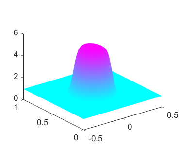
(a)	(b)	(c)

Figure 2: (a): numerical solution in $\Omega_{0}$; (b): the constructed local perturbation $q$; (c): the function $n+q$.

3 Explicit formulations of LAP solutions

In this section, we formulate the LAP solutions using two different methods introduced in [41] and [20], respectively. Note that the equation (1) can be rewritten as:

$$\Delta u+k^{2}nu=r\text{ in }\Omega,\quad\frac{\partial u}{\partial x_{2}}=0\text{ on }\partial\Sigma_{\pm}$$ (2)

where $r=f-k^{2}qu$, which depends on $u$, is compactly supported in $\Omega_{0}$. In this section, we extend the formulations of LAP solutions with purely periodic refractive indexes to periodic ones with local perturbations, and also prove the unique solvability of the formulations.

3.1 The $\alpha$-dependent periodic problems

From the Floquet theory, the $\alpha$-dependent periodic problems are particularly interesting as they are associated to the propagating modes (eigenfunctions). The strong formulation for the $\alpha$-dependent periodic problem is to find a periodic solution $v$ such that:

$$\Delta v+2\mathrm{i}\alpha\frac{\partial v}{\partial x_{1}}+(k^{2}n-\alpha^{2})v=g(x)\,\text{ in }\Omega_{0};\quad\frac{\partial v}{\partial x_{2}}=0\text{ on }\Sigma_{\pm}^{0},$$ (3)

where $g\in L^{2}(\Omega_{0})$. Note that $g=\mathcal{J}r=e^{-\mathrm{i}\alpha x_{1}}r$ (for the definition of $\mathcal{J}$ we refer to the end of this subsection), since $r$ is compactly supported in $\Omega_{0}$. For each $\alpha$, the weak formulation of the periodic problems is to find $v\in H^{1}_{per}(\Omega_{0})$ such that

$$\int_{\Omega_{0}}\left[\nabla v\cdot\nabla\overline{\psi}-\mathrm{i}\alpha\left(\frac{\partial v}{\partial x_{1}}\overline{\psi}-v\frac{\partial\overline{\psi}}{\partial x_{1}}\right)-(k^{2}n-\alpha^{2})v\overline{\psi}\right]\,\mathrm{d}x\,=-\int_{\Omega_{0}}g\overline{\psi}\,\mathrm{d}x\,$$ (4)

for any $\psi\in H^{1}_{per}(\Omega_{0})$. From Riesz representation theorem, there is an operator $A(\alpha,k):\,H^{1}_{per}(\Omega_{0})\rightarrow H^{1}_{per}(\Omega_{0})$ such that

$$\left<A(\alpha,k)\varphi,\psi\right>=\int_{\Omega_{0}}\left[\nabla\varphi\cdot\nabla\overline{\psi}-\mathrm{i}\alpha\left(\frac{\partial\varphi}{\partial x_{1}}\overline{\psi}-\varphi\frac{\partial\overline{\psi}}{\partial x_{1}}\right)-(k^{2}n-\alpha^{2})\varphi\overline{\psi}\right]\,\mathrm{d}x\,,$$

where $\left<\cdot,\cdot\right>$ is the inner product in the space $H^{1}_{per}(\Omega_{0})$. It is obvious that $A(\alpha,k)$ is a Fredholm operator (see [20]). When $k>0$ and $\alpha\in\mathbb{R}$, $A(\alpha,k)$ is a self-adjoint operator. There are operators $A_{1},A_{2},A_{3},A_{4}$ which do not depend on $\alpha$ and $k$ with obvious definitions such that

$$A(\alpha,k)=A_{1}+\alpha A_{2}+\alpha^{2}A_{3}+k^{2}A_{4}.$$ (5)

Thus $A(\alpha,k)$ depends analytically on both $\alpha$ and $k$. From [20], for fixed $k^{2}$, there are only finitely many $\alpha$’s in $[-\pi,\pi]$ such that $A(\alpha,k)$ is not invertible, which are called exceptional values. The set of exceptional values is denoted by $S(k)$. They are solutions of the quadratic eigenvalue problems for fixed $k$, thus can be computed in a standard way (for details we refer to Section 4.2). In the following, we introduce some definitions and notations concerning exceptional values without proofs. For details we refer to [5, 6, 12].

For any $\alpha\in[-\pi,\pi]$, there is a family of analytic functions $\mu_{i}(\alpha)$ defined in $[-\pi,\pi]$ such that:

$$(A_{1}+\alpha A_{2}+\alpha^{2}A_{3})\varphi=-\mu_{i}(\alpha)A_{4}.$$

For 2D periodic waveguide, none of the analytic functions is constant (see [12]). For any index $i$, the graph of the function $\mu_{i}$, i.e., $\{\big{(}\alpha,\mu_{i}(\alpha)\big{)}:\,\alpha\in[-\pi,\pi]\}$, is a dispersion curve. All the dispersion curves compose dispersion diagrams (see Figure 3).

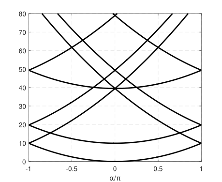
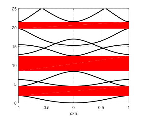
Figure 3: Dispersion diagrams for different $n$

For any fixed $k>0$, there is a finite set $I$ ( maybe empty, for example when $k^{2}$ lies in the red bands on the right picture of Figure 3) such that $S(k)=\Big{\{}\alpha\in[-\pi,\pi]:\,\exists\,i\in I,\,s.t.,\,\mu_{i}(\alpha)=k^{2}\Big{\}}$. Corresponding to each dispersion curve $\mu_{i}(\alpha)$, there is also a family of eigenfunctions $\{\varphi_{i}(\alpha,x):\,i\in I\}$ which also depend analytically on $\alpha$. When $\mu^{\prime}_{i}(\alpha)>0$ ($\mu^{\prime}_{i}(\alpha)<0$), then the corresponding eigenfunction $\varphi_{i}(\alpha,\cdot)$ propagates to the right (left); when $\mu^{\prime}_{i}(\alpha)=0$, then $\varphi_{i}(\alpha,\cdot)$ is a standing wave. For fixed $k>0$, $S(k)$ is divided into the following subsets:

$$S_{-}(k):=\left\{\alpha\in[0,2\pi]:\,\exists\,i\in I,\,s.t.,\,\mu_{i}(\alpha)=k^{2},\,\mu^{\prime}_{i}(\alpha)<0\right\};$$

$$S_{+}(k):=\left\{\alpha\in[0,2\pi]:\,\exists\,i\in I,\,s.t.,\,\mu_{i}(\alpha)=k^{2},\,\mu^{\prime}_{i}(\alpha)>0\right\};$$

$$S_{0}(k):=\left\{\alpha\in[0,2\pi]:\,\exists\,i\in I,\,s.t.,\,\mu_{i}(\alpha)=k^{2},\,\mu^{\prime}_{i}(\alpha)=0\right\}.$$

Note that when $S_{0}(k)\neq\emptyset$, the LAP does not work, so we have to make the following assumption.

Assumption 4.

In this paper, we assume that $S_{0}(k)=\emptyset$.

In [12], it has been proved that the positive valued $k$’s such that Assumptions 4 holds is only a discrete set, thus this assumption is reasonable.

At the end of this subsection, we apply the Floquet-Bloch transform to (1) (for details we refer to the appendix). Let us denote by $\mathcal{J}u$ the Floquet-Bloch transform of $u$ in $x_{1}$ direction (see Appendix), and set $v(\alpha,x):=(\mathcal{J}u)(\alpha,x)$ where $\alpha\in[-\pi,\pi]$. With formal calculation, $v(\alpha,\cdot)$ satisfies (3) and the solution $u$ is given by the inverse transform of $v$:

$$u(x)=\int_{-\pi}^{\pi}e^{\mathrm{i}\alpha x_{1}}v(\alpha,x)\,\mathrm{d}\alpha\,,\quad x\in\Omega_{0}.$$ (6)

From above arguments, (4) is uniquely solvable in $H^{1}_{per}(\Omega_{0})$ for all $\alpha\in[-\pi,\pi]\setminus S(k)$. From analytic Fredholm theory, the function $v$ is also extended to $\alpha\in\mathbb{C}$ (see Theorem 4 in [41]).

Theorem 5.

The Floquet-Bloch transformed field $v(\alpha,\cdot)=(\mathcal{J}u)(\alpha,\cdot)$ is extended to an analytic function for $\alpha\in\mathbb{C}\setminus\mathbb{F}$ (where $\mathbb{F}$ is a discrete set) and a meromorphic function for $\alpha\in\mathbb{C}$. Moreover, $e^{\mathrm{i}\alpha x_{1}}v(\alpha,\cdot)$ is periodic with respect to the real part of $\alpha$, i.e.,

$$e^{\mathrm{i}(\alpha+2\pi)x_{1}}v(\alpha+2\pi,\cdot)=e^{\mathrm{i}\alpha x_{1}}v(\alpha,\cdot),\quad\text{ for almost all }\alpha\in\mathbb{C}.$$

Note that when $S(k)\neq\emptyset$, $v(\alpha,\cdot)$ does not exist when $\alpha\in S(k)$ thus the inverse transform (6) is not well defined. The formulation (6) no longer works thus we need some modifications to give exact formulations for LAP solutions.

3.2 Complex contour integral method

In this subsection, we introduce the first method – the complex contour integral (CCI) method. To guarantee that the CCI method works, we have to make the following assumption.

Assumption 6.

Assume that $k>0$ such that $S_{-}(k)\cap S_{+}(k)=\emptyset$.

From [41], the positive valued $k$’s such that Assumptions 6 is satisfied is only a discrete set.

Remark 7.

Assumption 6 is actually not necessary for the LAP. For purely periodic case, the CCI method has been extended to the case without it in [41]. Concerning the length of this paper, we keep this assumption to only focus on the most important part.

Suppose that Assumption 4 and 6 are satisfied. The main idea of the CCI method is to modify the integral contour $[-\pi,\pi]$ in (6) such that the points in $S(k)$ are avoided. As the set $S(k)$ is finite, from the symmetry between $S_{+}(k)$ and $S_{-}(k)$ (see [41]), let

$$S_{+}(k)=\Big{\{}\widehat{\alpha}_{1}^{+},\dots,\widehat{\alpha}_{N}^{+}\Big{\}}\text{ and }S_{-}(k)=\Big{\{}\widehat{\alpha}_{1}^{-},\dots,\widehat{\alpha}_{N}^{-}\Big{\}}\quad\text{ where }{\widehat{\alpha}_{j}^{-}}=-\widehat{\alpha}_{j}^{+}.$$

First let the disk with center $\alpha$ and radius $\delta>0$ be denoted by $B(\alpha,\delta)$, and define

$$D_{\delta}:=\big{[}(-\pi,\pi)\times(0,+\infty)\big{]}\cup\left[\cup_{j=1}^{N}B\left(\widehat{\alpha}_{j}^{+},\delta\right)\right]\setminus\left[\cup_{j=1}^{N}\overline{B\left(\widehat{\alpha}_{j}^{-},\delta\right)}\right].$$

Define the new integral contour by:

$$\Lambda=\partial D_{\delta}\setminus\big{[}\{-\pi,\pi\}\times\mathbb{R}\big{]}.$$

With Assumption 4 and 6, we choose $\delta>0$ such that the following conditions are satisfied:

• any two disks do not have nonempty intersection;

• the closure of each disk only contains one exceptional value $\widehat{\alpha}_{j}^{\pm}$.

Suppose the problem (1) has an LAP solution $u\in H_{LAP}(\Omega)$, then $u$ is also the unique LAP solution of (2) with $r:=f-k^{2}qu$. In [41], the form of $u$ is given explicitly. Note that although $r$ depends on $u$, when $u$ is already a known LAP solution, we can still treat $r$ as some fixed function that is compactly supported in $\Omega_{0}$.

Theorem 8 (Theorem 7, [41]).

Assumption 4 and 6 hold. Then the LAP solution for (2) is given by

$$u(x):=\int_{\Lambda}e^{\mathrm{i}\alpha x_{1}}v(\alpha,x)\,\mathrm{d}\alpha\,,\quad x\in\Omega.$$ (7)

where $v(\alpha,\cdot)\in H^{1}_{per}(\Omega_{0})$ solves (4) for any fixed $\alpha\in\Lambda$ with $g(x)=e^{-\mathrm{i}\alpha x_{1}}r(x){=(\mathcal{J}r)(\alpha,x)}$.

Now we have to prove that with Assumption 2, 4 and 6, the problem (7) where $v(\alpha,\cdot)\in H^{1}_{per}(\Omega_{0})$ solves (4) for any fixed $\alpha\in\Lambda$ with $g(x)=e^{-\mathrm{i}\alpha x_{1}}\left(f(x)-k^{2}q(x)u(x)\right)$ has a unique solution in $H_{LAP}(\Omega)$, given any compactly supported $f\in L^{2}(\Omega_{0})$. Then the unique solution is the LAP solution for (1).

To describe the problem we first define the function space of the solution. Let $X:=L^{2}\left(\Lambda;H^{1}_{per}(\Omega_{0})\right)$. From the definition of $\Lambda$, the curve can be parameterized as $\Lambda:=\{s(t):=s_{1}(t)+\mathrm{i}s_{2}(t):\,t\in[0,1]\}$ where both $s_{1}$ and $s_{2}$ are real valued functions (for details we refer to Section 4.1). Then the norm of $X$ is defined as follows

$$\|\varphi\|_{X}=\left[\int_{0}^{1}\int_{\Omega_{0}}{\left[|\varphi(s(t),x)|^{2}+|\nabla_{x}\varphi(s(t),x)|^{2}\right]}|s^{\prime}(t)|\,\mathrm{d}x\,\,\mathrm{d}t\,\right]^{1/2}.$$

Since $v(\alpha,\cdot)$ satisfies(4), assume $\psi=\psi(\alpha,x)$ and integrating the equation on both sides with respect to $\alpha$ on the contour $\Lambda$, we arrive at the variational form of the problem.

The weak formulation is to find $v\in X$ such that

$$\int_{\Lambda}\left<A(\alpha,k)v(\alpha,\cdot),\psi(\alpha,\cdot)\right>\,\mathrm{d}\alpha\,=-\int_{\Lambda}\int_{\Omega_{0}}e^{-\mathrm{i}\alpha x_{1}}r(x)\overline{\psi(\alpha,x)}\,\mathrm{d}x\,\,\mathrm{d}\alpha\,$$

for all $\psi\in X$. From Riesz representation theorem, there is an operator ${\mathcal{A}}$ defined in $X$ such that

$$\left<{\mathcal{A}}\varphi,\psi\right>_{X}=\int_{\Lambda}\left<A(\alpha,k)\varphi(\alpha,\cdot),\psi(\alpha,\cdot)\right>\,\mathrm{d}\alpha\,,\quad\forall\,w,\,\psi\in X.$$

As any $\alpha\in\Lambda$ is not an exceptional value, $A(\alpha,k)$ is always invertible. Thus ${\mathcal{A}}$ is invertible in $X$.

As $r=f-k^{2}qu$, the variational formulation is written in the form:

$$\left<{\mathcal{A}}v,\psi\right>_{X}-k^{2}\int_{\Lambda}\int_{\Omega_{0}}e^{-\mathrm{i}\alpha x_{1}}q(x)u(x)\overline{\psi(\alpha,x)}\,\mathrm{d}x\,\,\mathrm{d}\alpha\,=-\int_{\Lambda}\int_{\Omega_{0}}e^{-\mathrm{i}\alpha x_{1}}f(x)\overline{\psi(\alpha,x)}\,\mathrm{d}x\,\,\mathrm{d}\alpha\,.$$ (8)

For simplicity, define the following operators. Let

$$({\mathcal{K}}v)(x):=\int_{\Lambda}e^{\mathrm{i}\alpha x_{1}}v(\alpha,x)\,\mathrm{d}\alpha\,,\quad x\in\Omega_{0}.$$

From Riesz representation theorem, there is an operator ${\mathcal{T}}$ in $H^{1}_{per}(\Omega_{0})$ such that

$$\left<{\mathcal{T}}\varphi,\psi\right>=\int_{\Omega_{0}}q(x)\varphi(x)\overline{\psi(x)}\,\mathrm{d}x\,,\,\text{ for any }\varphi,\,\psi\in H^{1}_{per}(\Omega_{0}).$$

As $H^{1}(\Omega_{0})$ is compactly embedded in $L^{2}(\Omega_{0})$, the operator ${\mathcal{T}}$ is also compact. Similarly, define $\mathcal{L}$ by:

$$\left<\mathcal{L}\varphi,\psi\right>=\int_{\Omega_{0}}\varphi(x)\overline{\psi(x)}\,\mathrm{d}x\,,\,\text{ for any }\varphi\in L^{2}(\Omega_{0}),\,\psi\in H^{1}_{per}(\Omega_{0}).$$

Then $\mathcal{L}$ is bounded from $L^{2}(\Omega_{0})$ to $H^{1}_{per}(\Omega_{0})$. Thus (8) is equivalent to

$$({\mathcal{A}}-k^{2}{\mathcal{K}}^{*}{\mathcal{T}}{\mathcal{K}}){v}=-{\mathcal{K}}^{*}\mathcal{L}f.$$ (9)

Now we study the property of the operator ${\mathcal{K}}$. We begin with a classical Minkowski integral inequality.

Lemma 9 ([13], Theorem 202).

Suppose $(S_{1},\mu_{1})$ and $(S_{2},\mu_{2})$ are two measure spaces and $F:S_{1}\times S_{2}\rightarrow\mathbb{R}$ is measurable. Then the following inequality holds for any $p\geq 1$

$$\left[\int_{S_{2}}\left|\int_{S_{1}}F(y,z)\,\mathrm{d}\mu\,_{1}(y)\right|^{p}\,\mathrm{d}\mu\,_{2}(z)\right]^{1/p}\leq\int_{S_{1}}\left(\int_{S_{2}}|F(y,z)|^{p}\,\mathrm{d}\mu\,_{2}(z)\right)^{1/p}\,\mathrm{d}\mu\,_{1}(y).$$ (10)

Lemma 10.

The operator ${\mathcal{K}}$ is bounded from $L^{2}(\Lambda;H^{m}(\Omega_{0}))$ to $H^{m}(\Omega_{0})$ for any fixed non-negative integer $m$. Especially, it is bounded from $X$ to $H^{1}(\Omega_{0})$.

Proof.

First consider the case when $m=0$. Given any $w\in C^{\infty}(\Lambda\times\Omega_{0})$, then ${\mathcal{K}}w$ is well defined and uniformly bounded for any $x\in\Omega_{0}$. Recall the parameterization of $\Lambda$,

$$\|{\mathcal{K}}w\|_{L^{2}(\Omega_{0})}=\left[\int_{\Omega_{0}}\left|\int_{\Lambda}e^{\mathrm{i}\alpha x_{1}}w(\alpha,x)\rm{d}\alpha\right|^{2}\,\mathrm{d}x\,\right]^{1/2}=\left[\int_{\Omega_{0}}\left|\int_{0}^{1}e^{\mathrm{i}s(t)x_{1}}w(s(t),x)s^{\prime}(t)\rm{d}t\right|^{2}\,\mathrm{d}x\,\right]^{1/2}.$$

Then from Lemma 9 (with $p=1$) and the Cauchy-Schwartz inequality,

$$\|{\mathcal{K}}w\|_{L^{2}(\Omega_{0})} =\left[\int_{\Omega_{0}}\left|\int_{0}^{1}e^{\mathrm{i}s(t)x_{1}}w(s(t),x)s^{\prime}(t)\rm{d}t\right|^{2}\,\mathrm{d}x\,\right]^{1/2}\leq\int_{0}^{1}\left(\int_{\Omega_{0}}|e^{\mathrm{i}s(t)x_{1}}w(s(t),x)|^{2}|s^{\prime}(t)|^{2}\,\mathrm{d}x\,\right)^{1/2}\,\mathrm{d}t\,$$

$$\leq\left(\int_{0}^{1}\int_{\Omega_{0}}|e^{\mathrm{i}s(t)x_{1}}w(s(t),x)|^{2}|s^{\prime}(t)|\,\mathrm{d}x\,\,\mathrm{d}t\,\right)^{1/2}\left({\int_{0}^{1}}|s^{\prime}(t)|\,\mathrm{d}t\,\right)^{1/2}\leq C\|w\|_{L^{2}(\Lambda;L^{2}(\Omega_{0}))}.$$

From the density of $C^{\infty}(\Lambda\times\Omega_{0})$ in $L^{2}(\Lambda;L^{2}(\Omega_{0}))$, the above inequality holds for all $w\in L^{2}(\Lambda;L^{2}(\Omega_{0}))$. Thus ${\mathcal{K}}$ is bounded from $L^{2}(\Lambda;L^{2}(\Omega_{j}))$ to $L^{2}(\Omega_{j})$. For $m\geq 1$, the proof is similar thus is omitted. So ${\mathcal{K}}$ is bounded from $L^{2}(\Lambda;H^{m}(\Omega_{0}))$ to $H^{m}(\Omega_{0})$ and particularly it is bounded from $X$ to $H^{1}(\Omega_{0})$. ∎

As ${\mathcal{A}}$ is invertible, ${\mathcal{K}}$ and ${\mathcal{T}}$ are bounded and ${\mathcal{T}}$ is compact, ${\mathcal{A}}-k^{2}{\mathcal{K}}^{*}{\mathcal{T}}{\mathcal{K}}$ is a Fredholm operator. Thus it is invertible if and only if it is an injection. Then we obtain the well-posedness of the problem (9) in the following theorem.

Theorem 11.

With Assumption 2, the operator ${\mathcal{A}}-k^{2}{\mathcal{K}}^{*}{\mathcal{T}}{\mathcal{K}}$ is invertible. That is, given any compactly supported $f\in L^{2}(\Omega_{0})$, the problem (9) has a unique solution in $X$.

Proof.

Suppose $v$ is a solution of (9) with $f=0$, i.e., $({\mathcal{A}}-k^{2}{\mathcal{K}}^{*}{\mathcal{T}}{\mathcal{K}})v=0$. Then $u={\mathcal{K}}v$ lies in $H^{1}(\Omega_{0})$. From [41], $u={\mathcal{K}}v$ is the LAP solution $r=-k^{2}qu$ in (2) thus it is the solution of (1) with $f=0$ and satisfies the radiation condition of Definition 1. From Assumption 2, $u=0$. Thus $v=0$, which implies that ${\mathcal{A}}-k^{2}{\mathcal{K}}^{*}{\mathcal{T}}{\mathcal{K}}$ is injective thus is invertible. So the problem (9) is well-posed in the space $X$. ∎

We have further regularity results for the solution ${v}$.

Corollary 12.

With Assumption 2, given any compactly supported $f\in L^{2}(\Omega_{0})$. The solution ${v}$ depends piecewise smoothly on $\alpha\in\Lambda$ and for fixed $\alpha$, ${v}(\alpha,\cdot)\in H^{2}_{per}(\Omega_{0})$.

Proof.

As for any $\alpha\in\Lambda$, $A(\alpha,k)$ is invertible and $\Lambda$ is a piecewise smooth curve, $A(\alpha,k)$ depends piecewise smoothly on $\alpha$ from the perturbation theory. For each fixed $\alpha\in\Lambda$, ${v}(\alpha,\cdot)\in H^{2}_{per}(\Omega_{0})$ from interior regularity.

∎

3.3 Decomposition method

In [18, 19] (also see [34], Chapter 5, paragraph 2), an explicit formulation of the radiation condition is given for periodic open tubes in 3D. However, since the method is easily transferred to this case, we introduce the decomposition method based on the definition without proofs. For simplicity, let

$$S(k):=\left\{\widehat{\beta}_{j}:\,j\in J\right\}\text{ where $J$ is a finite set}.$$

Although this set has already been introduced in previous subsections, we use different notations to indicate the elements in this set, just to avoid confusions. For any fixed $j$, the Fredholm operator $A(\widehat{\beta}_{j},k)$ is not an injection, and the null space $\widehat{Y}_{j}:=\mathcal{N}(A(\widehat{\beta}_{j},k))$ is finite dimensional with dimension $m_{j}$. There is an orthonormal eigensystem in $\widehat{Y}_{j}$

$$\Big{\{}(\lambda_{\ell,j},\widehat{\varphi}_{\ell,j}):\,\ell=1,2,\dots,m_{j}\Big{\}}$$ (11)

such that

$$\int_{\Omega_{0}}\left[-\mathrm{i}\frac{\partial\widehat{\varphi}_{\ell,j}}{\partial x_{1}}+\widehat{\beta}_{j}\widehat{\varphi}_{\ell,j}\right]\overline{\psi}\,\mathrm{d}x\,=\lambda_{\ell,j}k\int_{\Omega_{0}}n\widehat{\varphi}_{\ell,j}\overline{\psi}\,\mathrm{d}x\,\text{ for all }\psi\in\widehat{Y}_{j}$$ (12)

with normalization

$$2k\int_{\Omega_{0}}n\widehat{\varphi}_{\ell,j}\overline{\widehat{\varphi}_{\ell^{\prime},j}}\,\mathrm{d}x\,=\delta_{\ell,\ell^{\prime}}\text{ for }\ell,\ell^{\prime}=1,2,\dots,m_{j}.$$ (13)

Note that from the dispersion diagram, the positive integer $m_{j}$ indicates the number of dispersion curves that pass through the point $\left(\widehat{\beta}_{j},k^{2}\right)$. We can use the values of $\lambda_{\ell,j}$ to the direction of the eigenfunctions. When $\lambda_{\ell,j}>0$ ($<0$), the eigenfunction $\widehat{\varphi}_{\ell,j}$ propagates to the right (left) and $\widehat{\beta}_{j}\in S_{+}(k)$ ($S_{-}(k)$); when $\lambda_{\ell,j}=0$, $\widehat{\varphi}_{\ell,j}$ is a standing wave thus $\widehat{\beta}_{j}\in S_{0}(k)\neq\emptyset$. Since Assumption 4 holds, $\lambda_{\ell,j}\neq 0$ for all possible $\ell$ and $j$. In this case, it is possible that for some $j\in J$, $\lambda_{j,\ell}>0$ and $\lambda_{j,\ell^{\prime}}<0$ with $\ell\neq\ell^{\prime}$, which means Assumption 6 is not necessary for the decomposition method.

Let $\varphi_{\ell,j}:=e^{\mathrm{i}\widehat{\beta}_{j}x_{1}}{\widehat{\varphi}_{\ell,j}}$, then $\varphi_{\ell,j}$ is a $\widehat{\beta}_{j}$-quasi-periodic eigenfunction to the Helmholtz equation

$$\Delta\varphi_{\ell,j}+k^{2}n\varphi_{\ell,j}=0\text{ in }\Omega_{0};\quad\varphi_{\ell,j}=0\text{ on }\Sigma_{\pm}^{0}.$$

For each $j\in J$, let the space spanned by $\{\varphi_{\ell,j},\,\ell=1,2,\dots,m_{j}\}$ be denoted by $Y_{j}$.

With above notations, we are prepared to recall the radiation condition which is equivalent, but more explicit, compared to that defined in Definition 1.

Definition 13 (Theorem 3.7, [18]).

Suppose Assumption 2 and 4 hold.The LAP solution $u$ has a decomposition $u=u^{(1)}+u^{(2)}$ where $u^{(1)}\in H^{1}(\Omega)$ and $u^{(2)}$ has the form

$$u^{(2)}(x)=\psi^{+}(x_{1})\sum_{j\in{J}}\sum_{\lambda_{\ell,j}>0}f^{+}_{\ell,j}\varphi_{\ell,j}(x)+\psi^{-}(x_{1})\sum_{j\in{J}}\sum_{\lambda_{\ell,j}<0}f^{-}_{\ell,j}\varphi_{\ell,j}(x)$$ (14)

for some $f_{\ell,j}^{\pm}\in\mathbb{C}$ defined by (see [19])

$$f_{\ell,j}^{\pm}=f_{\ell,j}\ =\ \frac{\mathrm{i}}{|\lambda_{\ell,j}|}\int_{\Omega_{0}}r\,\overline{\varphi_{\ell,j}}\,\,\mathrm{d}x\,.$$ (15)

and

$$\psi^{+}(x_{1})\rightarrow 1\text{ as }x_{1}\rightarrow\infty,\,\psi^{+}(x_{1})\rightarrow 0\text{ as }x_{1}\rightarrow-\infty;\quad\psi^{-}(x_{1})=\psi^{+}(-x_{1}).$$

To simplify the representation, we assume that ${\rm supp}(q)\subset(-1/2+\delta,1/2-\delta)\times(0,1)$ for a $\delta\in(0,1/2)$, we can choose proper $\psi^{+}$ and $\psi^{-}$ such that $\psi^{\pm}(x_{1})q(x)=0$ for all $x\in\Omega$. For example, we can choose

$$\psi^{+}(x_{1})=1\text{ for }x_{1}\geq 1-\frac{\delta}{4}\text{ and }\psi^{+}(x_{1})=0\text{ for }x_{1}\leq 1-\frac{3\delta}{4}.$$

Replacing $u^{(2)}$ by its decomposition 14 in (2), we easily arrive at the following equation for $u^{(1)}$:

$$\Delta u^{(1)}+k^{2}nu^{(1)}={\mathcal{M}}(r),$$ (16)

where

$${\mathcal{M}}(r):=r-(\Delta+k^{2}n)u^{(2)}=r-\sum_{j\in J}\sum_{j=1}^{m}f_{\ell,j}\,g_{\ell,j}(x)$$

with the functions $g_{\ell,j}$ defined by:

$$g_{\ell,j}(x)=(\Delta+k^{2}n(x))\left[\psi^{\pm}(x_{1})\varphi_{\ell,j}(x)\right]=2(\psi^{\pm}(x_{1}))^{\prime}\frac{\partial\varphi_{\ell,j}}{\partial x_{1}}(x)+(\psi^{\pm}(x_{1}))^{{}^{\prime\prime}}\,\varphi_{\ell,j}(x)\text{ when }\pm\lambda_{\ell,j}>0.$$

From the property of $\psi^{\pm}$, ${\rm supp}\left(g_{\ell,j}\right)\subset\Omega_{0}$ for all $j$ and $\ell$, thus ${\mathcal{M}}(r)$ is also compactly supported in $\Omega_{0}$. It is easily checked that ${\mathcal{M}}$ is a bounded linear operator in $L^{2}\left(\Omega_{0}\right)$ and ${\rm ran}({\mathcal{M}})$ is orthogonal to $Y_{j}$ for any $j\in J$. For details we refer to Theorem 4.4 in [19].

Let $v(\beta,x):=\left(\mathcal{J}u^{(1)}\right)(\beta,x)$. Since $u^{(1)}$ decays exponentially as $|x_{1}|\rightarrow\infty$, $v(\beta,\cdot)\in H^{1}_{per}(\Omega_{0})$ exists for all $\beta\in[-\pi,\pi]$ and depends analytically on $\beta$ in the interval (and also extend analytically to a small neighbourhood of $[-\pi,\pi]$). For any fixed $\beta$, it is the unique solution of (4) with $r$ replaced by ${\mathcal{M}}(r)$.

Similarly to the CCI method, the weak formulation for the problem is to find $v\in L^{2}((-\pi,\pi);H^{1}_{per}(\Omega_{0}))$ such that

$$\int_{-\pi}^{\pi}\left<A(\beta,k)v(\beta,\cdot),{\psi(\beta,\cdot)}\right>\,\mathrm{d}\beta\,-k^{2}\int_{\Omega_{0}}{\mathcal{M}}\left(qu^{(1)}\right)\overline{\left(\int_{-\pi}^{\pi}e^{\mathrm{i}\beta x_{1}}\psi(\beta,x)\,\mathrm{d}\beta\,\right)}\,\mathrm{d}x$$ (17)

$$=-\int\limits_{\Omega_{0}}{\mathcal{M}}(f)\,\overline{\left(\int_{-\pi}^{\pi}e^{\mathrm{i}\beta x_{1}}\psi(\beta,x)\,\mathrm{d}\beta\,\right)}\,\,\mathrm{d}x\,.$$

Define the operator ${\mathcal{B}}$ by:

$$\left<{\mathcal{B}}v,\varphi\right>=\int_{-\pi}^{\pi}\left<A(\beta,k)v(\beta,x),{\varphi(\beta,x)}\right>\,\mathrm{d}\beta\,,\quad\text{ for all }v,\,\varphi\in L^{2}((-\pi,\pi);H^{1}_{per}(\Omega_{0})).$$

Then with the definition of ${\mathcal{T}}$ and $\mathcal{L}$ in the previous section, the variational form (17) is now equivalent to

$$\left({\mathcal{B}}-k^{2}\mathcal{J}{\mathcal{M}}{\mathcal{T}}\mathcal{J}^{-1}\right)v=-\mathcal{J}{\mathcal{M}}\mathcal{L}f.$$ (18)

As $A(\beta,k)$ is self-adjoint for real valued $\beta$, ${\mathcal{B}}$ is also self-adjoint. Thus the space $L^{2}((-\pi,\pi);H^{1}_{per}(\Omega_{0}))$ has the following decomposition:

$$L^{2}((-\pi,\pi);H^{1}_{per}(\Omega_{0}))={\rm ran}({\mathcal{B}})\oplus\ker({\mathcal{B}})\text{ and }{\rm ran}({\mathcal{B}})\bot\ker({\mathcal{B}}),$$

and ${\mathcal{B}}$ is an isomorphism from $Y:={\rm ran}({\mathcal{B}})$ to itself. Moreover, ${\rm ker}({\mathcal{B}})=\bigoplus_{j\in J}\widehat{Y}_{j}$. Since ${\rm ran}({\mathcal{M}})$ is orthogonal to all $Y_{j}$, ${\rm ran}(\mathcal{J}{\mathcal{M}})$ is orthogonal to $\widehat{Y}_{j}$, which implies that ${\rm ran}(\mathcal{J}{\mathcal{M}})\subset Y$. Thus the operator ${\mathcal{B}}-k^{2}\mathcal{J}{\mathcal{M}}{\mathcal{T}}\mathcal{J}^{-1}$ is an endomorphism of $Y$. As ${\mathcal{T}}$ is compact, the operator $\mathcal{J}{\mathcal{M}}{\mathcal{T}}\mathcal{J}^{-1}$ is a compact operator with range in $Y$. As ${\mathcal{B}}$ is invertible in $Y$, ${\mathcal{B}}-k^{2}\mathcal{J}{\mathcal{M}}{\mathcal{T}}\mathcal{J}^{-1}$ is a Fredholm operator. Thus we arrive at the well-posed result of (18).

Theorem 14.

Under assumption 2 and 4, then the operator ${\mathcal{B}}-k^{2}\mathcal{J}{\mathcal{M}}{\mathcal{T}}\mathcal{J}^{-1}$ is invertible in $Y$. Given any compactly supported $f\in L^{2}(\Omega_{0})$, the problem (18) has a unique solution in $Y$.

When $v$ is the unique solution of (18), then $u$ satisfies the radiation condition introduced in Definition 13. Thus it is the LAP solution for the problem (1).

Finally, we have to introduce a special technique for solving (18) numerically. Since $A(\beta,k)$ is not invertible in $H^{1}_{per}(\Omega_{0})$ when $\beta=\widehat{\beta}_{j}$, it is difficult to deal with such a point. To this end, we modify the formulation to avoid the singularities. Note that $v(\beta,\cdot)$ depends analytically on $\beta$ in $(-\pi-\delta,\pi+\delta)\times(-2\sigma,2\sigma)$ for sufficiently small $\delta,\,\sigma>0$. From Cauchy integral formula,

$$\oint_{C_{\sigma}}e^{\mathrm{i}\beta x_{1}}v(\beta,x)\,\mathrm{d}\beta\,=0,$$

where $C_{\sigma}$ is the boundary of the rectangle $[-\pi,\pi]\times[0,\sigma]$ which is oriented counter-clockwise. On the other hand, $e^{\mathrm{i}\beta x_{1}}v(\beta,\cdot)$ is $2\pi$-periodic with respect to the real part of $\beta$, this implies that the integrals on the left- and right edges cancel. Thus

$$\int_{-\pi}^{\pi}e^{\mathrm{i}\beta x_{1}}v(\beta,x)\,\mathrm{d}\beta\,=\int_{-\pi}^{\pi}e^{\mathrm{i}(\beta+\mathrm{i}\sigma)x_{1}}v(\beta+\mathrm{i}\sigma,x)\,\mathrm{d}\beta\,$$

where $v(\beta+\mathrm{i}\sigma,\cdot)$ solves (4) with parameter $\beta+\mathrm{i}\sigma$. In the numerical schemes, to avoid the singularities we always replace $\beta$ by $\beta+\mathrm{i}\sigma$ in the variational formulation (17).

4 Numerical schemes

In this section, we introduce two numerical schemes based on the two representations. For both methods, the periodic problems (4) are computed several times. So we briefly recall the finite element method for these problems at the very beginning.

Let ${\mathcal{M}}_{h}$ be a family of regular curved and quasi-uniform meshes which cover the domain $\Omega_{0}$. We also assume that the number and heights of nodal points on the left and right boundaries of $\Omega_{0}$ are the same, hence we can define functions that can be extended to periodic ones on the meshes. By omitting nodal points on the right boundary, we assume that the points $x_{j}$ ($j=1,2,\dots,M^{\prime}$) be all the nodal points, where $M^{\prime}$ is a positive integer. Let $M>M^{\prime}$ be a positive integer and $x_{j}$ ($j=M^{\prime}+1,\dots,M$) the points on the right boundary. Let $\{{\zeta}_{j}:\,j=1,2,\dots,M^{\prime}\}$ be the family of piecewise linear and globally continuous basis functions that vanish on $\Sigma_{\pm}^{0}$ defined on the meshes ${\mathcal{M}}_{h}$, and ${\zeta}_{j}(x_{\ell})=\delta_{j,\ell}$ where $j,\ell=1,2,\dots,M^{\prime}$ and where $\delta_{j,\ell}$ is the Kronecker delta function. Define the function $\zeta_{j}$ on $\Gamma_{1}$ by the value on $\Gamma_{0}$, then it is also extended periodically to $\Omega$ as a $1$-periodic function. Then we define the finite dimensional subspace:

$$V_{h}:={\rm span}\Big{\{}\zeta_{j}:\,j=1,2,\dots,M^{\prime}\Big{\}}\subset H^{1}_{per}(\Omega_{0}).$$

Then the solutions $v(\alpha,\cdot)$ are approximated in the finite dimensional subspace $V_{h}$.

In the next subsections, we introduce the two numerical methods based on formulations of the LAP solution by the complex contour integral and decomposition method. To simplify the process, we require the further assumption.

Assumption 15.

Assume that for any element $\alpha\in S(k)$, there is only one dispersion curve passing through $(\alpha,k^{2})$.

Note that although Assumption 15 is not necessary for both methods, the set with all the positive wave numbers such that Assumption 15 does not hold is only a zero set.

4.1 The CCI method

First we recall the variational form for the CCI method, i.e., find $v\in X$ such that

$$\begin{aligned} \int_{\Lambda}\left<A(\alpha,k)v(\alpha,\cdot),\psi(\alpha,\cdot)\right>\,\mathrm{d}\alpha\,-k^{2}\int_{\Lambda}\int_{\Omega_{0}}e^{-\mathrm{i}\alpha x_{1}}q(x)u(x)\overline{\psi(\alpha,x)}\,\mathrm{d}x\,\,\mathrm{d}\alpha\,\\ =-\int_{\Lambda}\int_{\Omega_{0}}e^{-\mathrm{i}\alpha x_{1}}f(x)\overline{\psi(\alpha,x)}\,\mathrm{d}x\,\,\mathrm{d}\alpha\,\end{aligned}$$ (19)

$$u(x)=\int_{\Lambda}e^{{\mathrm{i}\alpha x_{1}}}v(\alpha,x)\,\mathrm{d}\alpha\,.$$ (20)

In this subsection, we focus of the discretization of the curve $\Lambda$. The modified integral contour $\Lambda$ is composed of a finite number of intervals and semicircles, then the first step is to parameterize $\Lambda$ piecewisely:

$$\Lambda=\cup_{j=1}^{Q}\overline{\Big{\{}s_{j}(t)=s_{j}^{1}(t)+\mathrm{i}s^{2}_{j}(t):\,t\in I_{j}\Big{\}}},$$

where $I_{j}$ are closed bounded intervals. For each fixed $j=1,2\dots,Q$, $s_{j}^{1}$ and $s^{2}_{j}$ are real smooth functions on the interval $I_{j}$. With a proper parameterization, let the intervals $I_{1},\dots,I_{Q}$ be

$$I_{1}=(0,a_{1}),\,I_{2}=(a_{1},a_{2}),\dots,I_{j}=(a_{j-1},a_{j}),\dots,I_{Q}=(a_{Q-1},a_{Q})=(a_{Q-1},1),$$

then

$$\Lambda=\Big{\{}s(t)=s_{1}(t)+\mathrm{i}s_{2}(t):\,t\in[0,1]\Big{\}}$$

where $s_{1}=s_{j}^{1}$ and $s_{2}=s_{j}^{2}$ in each $I_{j}$, respectively. Since the trapezoidal rule converges much faster for smooth periodic functions than nonperiodic smooth functions (see [39]), we require

$$s^{(m)}_{j}\left(a_{j-1}\right)=s^{(m)}_{j}\left(a_{j}\right)=0,\quad\forall\,j=1,2,\dots,Q\text{ and }m=1,2.$$

Then $s^{\prime}(t)$ is smooth in $[0,1]$ and it can be extended to a periodic smooth function in $\mathbb{R}$. For details of this technique we refer to Section 9.6 in [22].

Replacing $\alpha$ by $s(t)$ in the equations (19)-(20) and letting $\widetilde{v}(t,x):=v(s(t),x)s^{\prime}(t)$, we arrive at the following equivalent equations:

$$\begin{aligned} \int_{0}^{1}\left<A(s(t),k)\widetilde{v}(t,\cdot),\psi(t,\cdot)\right>\,\mathrm{d}t\,-k^{2}\int_{0}^{1}\int_{\Omega_{0}}e^{-\mathrm{i}s(t)x_{1}}q(x)u(x)\overline{\psi(t,x)}s^{\prime}(t)\,\mathrm{d}x\,\,\mathrm{d}t\,\\ =-\int_{0}^{1}\int_{\Omega_{0}}e^{-\mathrm{i}s(t)x_{1}}f(x)\overline{\psi(t,x)}s^{\prime}(t)\,\mathrm{d}x\,\,\mathrm{d}t\,,\end{aligned}$$ (21)

$$u(x)=\int_{0}^{1}e^{\mathrm{i}s(t)x_{1}}\widetilde{v}(t,x)\,\mathrm{d}t\,.$$ (22)

The variational problem is to seek $\widetilde{v}\in\widetilde{X}:=L^{2}\left((0,1);H^{1}_{per}(\Omega_{0})\right)$ such that (21)-(22) hold for all test function $\psi\in\widetilde{X}$. From Corollary 12, $\widetilde{v}\in C^{\infty}_{per}\left([0,1];H^{2}_{per}(\Omega_{0})\right)$.

Now we discretize the system (21)-(22). As the finite element discretization in the domain $\Omega_{0}$ has already been introduced at the beginning of this section, we only introduce the trigonometric interpolation in the domain $[0,1]$. Let $N$ be a positive integer and the uniformly distributed nodal points be

$$t_{0}=0;\quad t_{j}=\frac{j}{N}\quad\forall\,j=1,2,\dots,N.$$

Suppose $N$ is an even number, then let us introduce the basic functions:

$$\xi_{\ell}(t):=\frac{1}{N}\sum_{m=-N/2+1}^{N/2}\exp\left(\mathrm{i}2\pi m(t-t_{\ell})\right),\,\ell=1,2,\dots,N.$$

It is well known that

$$\xi_{\ell}(t_{\ell^{\prime}})=\delta_{\ell,\ell^{\prime}}\text{ and }\int_{0}^{1}\xi_{\ell}(t)\xi_{\ell^{\prime}}(t)\,\mathrm{d}t\,=\frac{1}{N}\delta_{\ell,\ell^{\prime}}.$$

Now we are prepared to discretize the system (21)-(22) in the finite dimensional space:

$$\widetilde{X}_{N,h}:=\underbrace{V_{h}\bigoplus V_{h}\bigoplus\cdots\bigoplus V_{h}}_{N\text{ spaces }}.$$

Let $\widetilde{v}_{N,h}\in\widetilde{X}_{N,h}$ be the approximation of $\widetilde{v}$ of the form:

$$\widetilde{v}_{N,h}(t,x)=\sum_{\ell=1}^{N}\sum_{j=1}^{M}\widehat{v}_{\ell,j}\xi_{\ell}(t)\zeta_{j}(x),$$

then

$$u_{N,h}(x)=\sum_{j=1}^{M}\widehat{u}_{j}\zeta_{j}(x)\text{ where }\widehat{u}_{j}=\frac{1}{N}\sum_{\ell=1}^{N}e^{\mathrm{i}s(t_{\ell})x_{1}}\widehat{{v}}_{\ell,j}.$$ (23)

With the test function $\psi(t,x)=\xi_{\ell^{\prime}}(t)\zeta_{j^{\prime}}(x)$, (21)-(22) is discretized as:

$$\frac{1}{N}\delta_{\ell,\ell^{\prime}}\sum_{j=1}^{M^{\prime}}\widehat{v}_{\ell,j}\left<A(t_{\ell},k)\zeta_{j},\zeta_{j^{\prime}}\right>-\frac{k^{2}}{N}\sum_{j=1}^{{M^{\prime}}}\widehat{u}_{j}\left(\int_{\Omega_{0}}e^{-\mathrm{i}s(t_{\ell^{\prime}})x_{1}}q(x)\zeta_{j}(x){\zeta_{j^{\prime}}(x)}\,\mathrm{d}x\,\right)s^{\prime}(t_{\ell^{\prime}})$$ (24)

$$=-\frac{1}{N}\left(\int_{\Omega_{0}}e^{-\mathrm{i}s(t_{\ell^{\prime}})x_{1}}f(x)\zeta_{j^{\prime}}(x)\,\mathrm{d}x\,\right)s^{\prime}(t_{\ell^{\prime}}).$$

With (23) we also get the approximation of $u$, i.e., $u_{N,h}$, at the same time.

Finally the system (23)-(24) is summarized by the following system:

$$\left(\begin{matrix}A_{1}&0&\cdots&0&C_{1}\\ 0&A_{2}&\cdots&0&C_{2}\\ \vdots&\vdots&\ddots&\vdots&\vdots\\ 0&0&\cdots&A_{N}&C_{N}\\ B_{1}&B_{2}&\cdots&B_{N}&I\end{matrix}\right)\left(\begin{matrix}V_{1}\\ V_{2}\\ \vdots\\ V_{N}\\ U\end{matrix}\right)=\left(\begin{matrix}F_{1}\\ F_{2}\\ \vdots\\ F_{N}\\ 0\end{matrix}\right),$$ (25)

where $V_{j}=\left(\widehat{v}_{1,j},\dots,\widehat{v}_{M,j}\right)^{\top}$ and $U=\left(\widehat{u}_{1},\dots,\widehat{u}_{M}\right)^{\top}$. $A_{j}$ comes from the first term of (24), $C_{j}$ comes from the second term of (24), $B_{j}$ comes from (23), $F_{j}$ comes from the right hand side. The size of this system is $(N+1)M\times(N+1)M$. Note that $U$ is treated as an additional unknown vector just for a simpler representation of the linear system. Then the final task is to solve the linear sparse system with the size $(N+1)M\times(N+1)M$.

4.2 The decomposition method

We introduce the decomposition method in this subsection. Since Assumption 15 holds, $m_{j}=1$ for all $j\in J$, so we abbreviate the notations $\lambda_{\ell,j},\,\varphi_{\ell,j},\,g_{\ell,j}$ as $\lambda_{j},\,\varphi_{j},\,g_{j}$. First we define

$$f_{0}(x):={\mathcal{M}}(f)=f-\sum_{j\in J}\frac{\mathrm{i}}{|\lambda_{j}|}\left[\int_{\Omega_{0}}f(x)\overline{\varphi_{j}}\,\mathrm{d}x\,\right]g_{j}(x).$$ (26)

We simplify the second term in (17):

$$\int_{\Omega_{0}}{\mathcal{M}}\left(qu^{1}\right)\overline{\int_{-\pi}^{\pi}e^{\mathrm{i}\beta x_{1}}\psi(\beta,x)\,\mathrm{d}\beta\,}\,\mathrm{d}x\,=\int_{\Omega_{0}}u^{(1)}(x)\overline{\theta(x;\psi)}\,\mathrm{d}x\,$$

where $\theta(x;\psi)=q(x){\mathcal{M}}^{*}\left[\int_{-\pi}^{\pi}e^{\mathrm{i}\beta x_{1}}\psi(\beta,x)\,\mathrm{d}\beta\,\right]$ and ${\mathcal{M}}^{*}$ is the adjoint operator of ${\mathcal{M}}$ defined as:

$${\mathcal{M}}^{*}(f)=f(x)+\sum_{j\in J}\frac{\mathrm{i}}{|\lambda_{j}|}\varphi_{j}(x)\left[\int_{\Omega_{0}}\overline{g_{j}(y)}f(y)\,\mathrm{d}y\,.\right]$$

From the variational form (17) (note that $\beta$ is already replaced by $\beta+\mathrm{i}\sigma$):

$$\begin{aligned} \int_{-\pi}^{\pi}\left<A(\beta+\mathrm{i}\sigma,k)v(\beta{+\mathrm{i}\sigma},\cdot),\psi(\beta{+\mathrm{i}\sigma},\cdot)\right>\,\mathrm{d}\beta\,-k^{2}\int_{\Omega_{0}}u^{(1)}(x)\overline{\theta(x;\psi)}\,\mathrm{d}x\,\\ =-\int_{-\pi}^{\pi}\int_{\Omega_{0}}e^{-\mathrm{i}(\beta+\mathrm{i}\sigma)x_{1}}f_{0}(x)\overline{\psi(\beta{+\mathrm{i}\sigma},x)}\,\mathrm{d}x\,\,\mathrm{d}\beta\,;\end{aligned}$$ (27)

$$u^{(1)}(x)=\int_{-\pi}^{\pi}e^{\mathrm{i}(\beta+\mathrm{i}\sigma)x_{1}}v(\beta+\mathrm{i}\sigma,x)\,\mathrm{d}\beta\,.$$ (28)

To discretize (27)-(28), the first step is to approximate the exceptional values $\widehat{\beta}_{j}$ and the corresponding systems $\left\{\left(\lambda_{j},\widehat{\varphi}_{j}\right)\right\}$. This implementation is carried out by the following two steps. The first step is to find all the real eigenvalues and corresponding eigenspaces of the quadratic pencil $A(\alpha,k)=A_{1}+k^{2}A_{4}+\alpha A_{2}+\alpha^{2}A_{3}$ (see (5)). The operators are discretized by the finite element method and let $A_{1}^{h},A_{2}^{h},A_{3}^{h},A_{4}^{h},B_{1}^{h},B_{2}^{h}$ be the corresponding matrices. A standard way to solve above quadratic eigenvalue problem is to solve the following linearized problems:

$$B_{1}^{h}W^{h}=\lambda B_{2}^{h}W^{h},$$ (29)

where

$$B_{1}^{h}:=\left(\begin{matrix}A_{1}^{h}+k^{2}A_{4}^{h}&0\\ 0&I\end{matrix}\right),\quad B_{2}^{h}=\left(\begin{matrix}-A_{2}^{h}&-A_{3}^{h}\\ I&0\end{matrix}\right).$$

By solving this problem, we find all the eigenvalues and eigenfunctions

$$\left\{\left(\widehat{\beta}_{j}^{h},\widehat{\varphi}_{j}^{h}\right):\,j\in J^{h}\right\}.$$

We normalize the function $\widetilde{\varphi}_{j}^{h}$ by

$$2k\int_{\Omega_{0}}n(x)\widehat{\varphi}^{h}_{j}(x)\overline{\widehat{\varphi}^{h}_{j}(x)}\,\mathrm{d}x\,=1.$$

Since the discretized matrices approximate the exact ones when $h\rightarrow 0$, for sufficiently small $h>0$, $J^{h}=J$ and

$$\left|\widehat{\beta}_{j}^{h}-\widehat{\beta}_{j}\right|=O(h^{2}),\quad\left\|\widehat{\varphi}_{j}^{h}-\widehat{\varphi}_{j}\right\|_{H^{1}_{per}(\Omega_{0})}=O(h)$$

hold for all $j\in J$. For details of the error estimation we refer to [21, 1, 7]. When Assumption 15 no longer holds, we refer to the Appendix for details.

Using (12) we also get the parameter $\lambda_{j}^{h}$. Let $\varphi^{h}_{j}(x):=e^{\mathrm{i}\widehat{\beta}_{j}^{h}x_{1}}\widehat{\varphi}^{h}_{j}(x)$, then the system $\Big{\{}(\lambda^{h}_{j},\varphi^{h}_{j})\Big{\}}$ for fixed $j\in J$ is the numerical approximation of (11) with the following convergence result:

$$\left|\lambda^{h}_{j}-\lambda_{j}\right|=O(h^{2}),\quad\left\|{\varphi}_{j}^{h}-{\varphi}_{j}\right\|_{H^{1}(\Omega_{0})}=O(h).$$ (30)

With these values and functions, we get the function $\theta^{h}(x;\psi)$ by replacing $\lambda_{j}$, $\varphi_{j}$ by $\lambda_{j}^{h}$, $\varphi_{j}^{h}$.

Now we are prepared to discretize the system (27)-(28) with $\theta(x;\psi)$ replaced by $\theta^{h}(x;\psi)$, and $f_{0}(x)$ replaced by $f_{0}^{h}(x)$. The related solutions are denoted by $v_{h}(\beta,x)$ and $u^{(1)}_{h}(x)$. With this substitution, $u$ reads:

$$u(x)=u^{(1)}_{h}(x)+u^{(2)}_{h}(x)$$ (31)

where $u^{({1})}_{h}$ solves

$$\Delta u^{({1})}_{h}+k^{2}nu^{({1})}_{h}=\sum_{j\in J}\frac{\mathrm{i}}{|\lambda_{j}^{h}|}\int_{\Omega_{0}}f(x)\overline{\varphi_{j}^{h}(x)}\,\mathrm{d}x\,g_{j}^{h}(x)$$

and $g_{j}^{h}$ is defined in the same way as $g_{j}$ replacing $\varphi_{j}$ by $\varphi_{j}^{h}$. Let $g$ be a complex valued smooth function defined in $[0,1]$ such that $g(t)=\mathrm{Re}\,(g(t))+\mathrm{i}\sigma$ and

$$\mathrm{Re}\,(g(0))=-\pi\text{ and }\mathrm{Re}\,(g(1))=\pi,\quad g^{(m)}(0)=g^{(m)}(1)=0\quad\text{for all }\,m=1,2,\dots.$$

Replace $\beta+\mathrm{i}\sigma$ by $g(t)$ in (27)-(28) and $\theta(x;\psi)$ by $\theta^{h}(x;\psi)$, and define $\widetilde{v}(t,x):=v^{h}(g(t),x)g^{\prime}(t)$, then $\widetilde{v}\in C^{\infty}_{per}\left([0,1];H^{2}_{per}(\Omega_{0})\right)$. We arrive at the variational form for $\widetilde{v}$, i.e., find $\widetilde{v}\in L^{2}\left((0,1);H^{1}_{per}(\Omega_{0})\right)$ such that

$$\begin{aligned} \int_{0}^{1}\left<A(g(t),k)\widetilde{v}(t,\cdot),\psi(t,\cdot)\right>\,\mathrm{d}t\,-k^{2}\int_{\Omega_{0}}u^{(1)}_{h}(x)\overline{\theta^{h}(x;\psi)}\,\mathrm{d}x\,\\ =-\int_{0}^{1}\int_{\Omega_{0}}e^{-\mathrm{i}g(t)x_{1}}f_{0}^{h}(x)\overline{\psi(t,x)}g^{\prime}(t)\,\mathrm{d}x\,\,\mathrm{d}t\,;\end{aligned}$$ (32)

$$u^{(1)}_{h}(x)=\int_{0}^{1}e^{\mathrm{i}g(t)x_{1}}\widetilde{v}(t,x)\,\mathrm{d}t\,.$$ (33)

Here $f_{0}^{h}$ is defined in (26) by replacing $\varphi_{j}$ by $\varphi^{h}_{j}$.

We use the same discretization as in the CCI method and consider the discretized problem in the space $\widetilde{X}_{N,h}$, where $\widetilde{v}_{N,h}\subset\widetilde{X}_{N,h}$ is given by:

$$\widetilde{v}_{N,h}=\sum_{\ell=1}^{N}\sum_{j=1}^{M}\widehat{v}_{\ell,j}\xi_{\ell}(t)\zeta_{j}(x).$$

Then

$$u^{(1)}_{N,h}=\sum_{j=1}^{M}\widehat{u}_{j}\zeta_{j}(x)\text{ where }\widehat{u}_{j}=\frac{1}{N}\sum_{\ell=1}^{N}e^{\mathrm{i}g(t_{\ell})x_{1}}\widehat{v}_{\ell,j}$$ (34)

With the test function $\psi(t,x)=\xi_{\ell^{\prime}}(t)\zeta_{j^{\prime}}(x)$, we get the discretized form of the system (32)-(33):

$$\frac{1}{N}\delta_{\ell,\ell^{\prime}}\sum_{j=1}^{M}\widehat{v}_{\ell,j}\left<A(t_{\ell},k)\zeta_{j},\zeta_{j^{\prime}}\right>-k^{2}\sum_{j=1}^{M}\widehat{u}_{j}\left(\int_{\Omega_{0}}\zeta_{j}(x)\overline{\theta(x;\xi_{\ell^{\prime}}(t)\zeta_{j^{\prime}}(x))}\,\mathrm{d}x\,\right)$$ (35)

$$=-\frac{1}{N}\left(\int_{\Omega_{0}}e^{-\mathrm{i}g(t_{\ell^{\prime}})x_{1}}f_{0}^{h}(x)\overline{\zeta_{j^{\prime}}(x)}\,\mathrm{d}x\,\right)g^{\prime}(t_{\ell^{\prime}}).$$

As in the CCI method, we approximate $u^{(1)}_{h}$ by $u^{(1)}_{N,h}$ with coefficients defined by (34). Finally the system (34)-(35) is summarized by the following system:

$$\left(\begin{matrix}\widetilde{A}_{1}&0&\cdots&0&\widetilde{C}_{1}\\ 0&\widetilde{A}_{2}&\cdots&0&\widetilde{C}_{2}\\ \vdots&\vdots&\ddots&\vdots&\vdots\\ 0&0&\cdots&\widetilde{A}_{N}&\widetilde{C}_{N}\\ \widetilde{B}_{1}&\widetilde{B}_{2}&\cdots&\widetilde{B}_{N}&I\end{matrix}\right)\left(\begin{matrix}V_{1}\\ V_{2}\\ \vdots\\ V_{N}\\ U\end{matrix}\right)=\left(\begin{matrix}\widetilde{F}_{1}\\ \widetilde{F}_{2}\\ \vdots\\ \widetilde{F}_{N}\\ 0\end{matrix}\right),$$ (36)

where $\widetilde{A}_{j}$ comes from the first term of (35), $\widetilde{C}_{j}$ comes from the second term of (35), $\widetilde{B}_{j}$ comes from (34), $\widetilde{F}_{j}$ comes from the right hand side. The size of this system is $(N+1)M\times(N+1)M$.

4.3 Error estimations

In the last part of this section, we present the error estimations for both algorithms. Since both solutions $\widetilde{w}(t,x)$ of (21)-(22) and the solution $\widetilde{v}(t,x)$ of (32)-(33) lie in the space $C^{\infty}_{per}\left([0,1];H^{2}_{per}(\Omega_{0})\right)$, we can use the error estimation given in [40]. The first result is the error estimation of the interpolation in the finite dimensional space $\widetilde{X}_{N,h}$. Combining equation (32) in [40] and (46) in [28], we have the following results.

Theorem 16.

Suppose $v\in C^{\infty}_{per}\left([0,1];H^{2}_{per}(\Omega_{0})\right)$ and $v_{N,h}$ is the interpolation of $v$ in the subspace $\widetilde{X}_{N,h}$. Then

$$\min_{v_{N,h}\in\widetilde{X}_{N,h}}\|v-v_{N,h}\|_{L^{2}\left([0,1];H^{1}_{per}(\Omega_{0})\right)}\leq C\left(N^{-n}+h\right)\|v\|_{C^{\infty}_{per}\left([0,1];H^{2}_{per}(\Omega_{0})\right)},$$

where $n$ can be any positive integer and $C$ depending on $\|v\|_{C^{n}([0,1];H^{2}_{per}(\Omega_{0}))}$ .

This implies that the interpolation decays super algebraically with respect to the parameter $1/N$ but linearly with respect to $h$. With this result, we get the error estimations for finite element solutions of the variational problems (21)-(22) and (32)-(33).

Theorem 17 (Theorem 4, [40]).

Let $\widetilde{w}$ be the exact solution of (21)-(22) and $\widetilde{w}_{N,h}$ be the finite element solution of the corresponding discretized form (23)-(24). Let $\widetilde{v}$ be the exact solution of (32)-(33) and $\widetilde{v}_{N,h}$ be the finite element solution of (34)-(35). For sufficiently small $h>0$ and sufficiently large positive integer $N$, we have the following error estimations:

$$\left\|\widetilde{w}-\widetilde{w}_{N,h}\right\|_{L^{2}([0,1]\times\Omega_{0})}\leq Ch\left(N^{-n}+h\right)\|\widetilde{w}\|_{C^{\infty}_{per}\left([0,1];H^{2}_{per}(\Omega_{0})\right)};$$ (37)

$$\left\|\widetilde{v}-\widetilde{v}_{N,h}\right\|_{L^{2}([0,1]\times\Omega_{0})}\leq Ch\left(N^{-n}+h\right)\|\widetilde{v}\|_{C^{\infty}_{per}\left([0,1];H^{2}_{per}(\Omega_{0})\right)}$$ (38)

where $C$ is a parameter depending on $n$.

For both methods, we get the original solution from (23), and the error is also easily obtained:

$$\left\|u-u_{N,h}\right\|_{L^{2}(\Omega_{0})}\leq Ch\left(N^{-n}+h\right)\|\widetilde{v}\|_{C^{\infty}_{per}\left([0,1];H^{2}_{per}(\Omega_{0})\right)};$$ (39)

$$\left\|u^{(1)}_{h}-u^{(1)}_{N,h}\right\|_{L^{2}(\Omega_{0})}\leq Ch\left(N^{-n}+h\right)\|\widetilde{v}\|_{C^{\infty}_{per}\left([0,1];H^{2}_{per}(\Omega_{0})\right)}.$$ (40)

For the CCI method, the final error estimation is already obtained by (39). Then in the following, we mainly focus on the decomposition method.

Recall (30), we have the error bound $\left\|u^{(1)}-u^{(1)}_{h}\right\|_{L^{2}(\Omega_{0})}\leq O(h)$, which converges only linearly with respect to $h$. However, recall (31),

$$u(x)=u^{(1)}_{h}(x)+u^{(2)}_{h}(x)$$

and the numerical solution is given by

$$u_{N,h}=u^{(1)}_{N,h}(x)+u^{(2)}_{h}(x).$$

Finally we get the error estimate for the decomposition method:

$$\left\|u-{u}_{N,h}\right\|_{L^{2}(\Omega_{0})}=\left\|u^{(1)}_{h}-u^{(1)}_{N,h}\right\|_{L^{2}(\Omega_{0})}\leq Ch\left(N^{-n}+h\right)\|\widetilde{v}\|_{C^{\infty}_{per}\left([0,1];H^{2}_{per}(\Omega_{0})\right)}.$$ (41)

5 Numerical examples

In this section, we give some numerical examples to show the efficiency of both methods. For both cases, we apply the same finite element discretization for quasi-periodic problem (4), and the meshsize $h$ is chosen as $0.005,0.01,0,02,0,04$. The parameter $N$ is chosen as $4,8,16,32,64$.

We show numerical results for two different examples. For both examples, $f$ and $q$ are the same. $f$ is already defined in Remark 2, and $q$ is defined by:

$$q(x)=\begin{cases}0,\quad|x-b_{0}|>0.15;\\ 2,\quad 0.1<|x-b_{0}|<0.15;\\ 2\zeta(|x-b_{0}|;0.1,0.15),\quad\text{otherwise.}\end{cases}$$

where $b_{0}=(0.2,0.2)^{\top}$. In Example 1, the periodic refractive index $n=n_{1}$ is defined also in Remark 2, while in Example 2,

$$n(x)=n_{2}(x)=3+\sin(4\pi x_{1}).$$

The wave number is chosen as $\sqrt{17}$ in Example 1 and $\sqrt{12}$ in Example 2. We plot the dispersion diagrams for both examples in Figure 4. From the diagrams we get the set of exceptional values: For Example 1,

$$S(k)=\big{\{}-0.9577,\,0.9577\big{\}}\text{ and }S_{-}(k)=\big{\{}-0.9577\big{\}},\,S_{+}(k)=\big{\{}0.9577\big{\}};$$

while for Example 2,

$$S(k)=\big{\{}-1.0326,\,1.0326\big{\}}\text{ and }S_{-}(k)=\big{\{}1.0326\big{\}},\,S_{+}(k)=\big{\{}-1.0326\big{\}}.$$

Note that since the above results are numerical, they are not exact. Based on the exceptional values, we also show the integral contour $\Lambda$ in Figure 5.

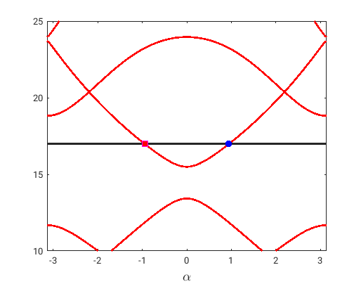
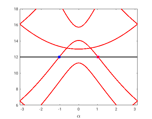
(a)	(b)

Figure 4: Dispersion diagrams: Example 1 in (a) and Example 2 in (b). Blue dots are points in $S_{+}(k)$ and purple squares are points in $S_{-}(k)$.

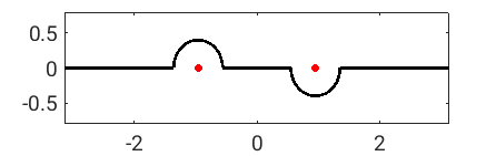
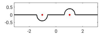
(a)	(b)

Figure 5: Integral contour $\Lambda$: Example 1 in (a) and Example 2 in (b). Red dots exceptional values.

5.1 The convergence of exceptional values

First, we show the convergence of the approximated exceptional values with respect to the meshsize $h$. As the convergence of eigenfunctions and $\lambda_{\ell,j}^{h}$ are similar, they are omitted here. For $h=0.04,0.02,0.01,0.005$, we compute the exceptional values and the positive ones are listed in Table 1.

	$h=0.04$	$h=0.02$	$h=0.01$	$h=0.005$
Example 1	0.8982	0.9435	0.9549	0.9577
Example 2	1.0738	1.0387	1.0337	1.0326

Table 1: Positive exceptional values computed with different $h$’s.

If the values at $h=0.005$ is treated as “exact”, then we plot the relative error with respect to the parameter $h$ in logarithmic scales in the first picture in Figure 6. From the plot, the slope of the red curve is about $2.2$ and that of the blue one is about $2.6$, which corresponds to (and even a little faster than) the convergence of the finite element method. Thus the convergence rates for the exceptional values are even faster than expected, i.e., $O(h^{2})$.

5.2 Numerical results

In this section, we focus on the numerical results obtained by the proposed methods. For both examples, we use a completely different method given in [6] to produce “exact solutions”. In the computation we use Lagrangian element with meshsize $0.005$ and an extrapolation technique with data points $0.001,0.0005,0.00025$, and the solution is denoted by $u_{exa}$. Then the error is estimated as:

$$err_{N,h}=\frac{\|u_{N,h}-u_{exa}\|_{L^{2}(\Omega_{0})}}{\|u_{exa}\|_{L^{2}(\Omega_{0})}}.$$

For the decomposition method, the parameter $\sigma$ is chosen to be $0.2$. For the relative errors with different examples and methods we refer to Table 2-5. From the four tables, the relative errors decrease as $h$ gets smaller and $N$ gets larger, but the decrease stops at the level of $3\times 10^{-3}$. This may due to the lack of accuracy of the “exact solutions”.

	$h=0.04$	$h=0.02$	$h=0.01$	$h=0.005$
$N=16$	$1.98$E$-1$	$1.85$E$-1$	$1.80$E$-1$	$1.78$E$-1$
$N=32$	$8.87$E$-2$	$5.26$E$-2$	$4.30$E$-2$	$4.06$E$-2$
$N=64$	$6.21$E$-2$	$1.96$E$-2$	$7.54$E$-3$	$4.60$E$-3$
$N=128$	$6.12$E$-2$	$1.87$E$-2$	$6.60$E$-3$	$3.82$E$-3$
$N=256$	$6.12$E$-2$	$1.87$E$-2$	$6.60$E$-3$	$3.82$E$-3$

Table 2: Relative error for Example 1, CCI method.

	$h=0.04$	$h=0.02$	$h=0.01$	$h=0.005$
$N=16$	$7.89$E$-2$	$2.00$E$-2$	$5.42$E$-3$	$3.13$E$-3$
$N=32$	$8.27$E$-2$	$2.05$E$-2$	$5.44$E$-3$	$3.09$E$-3$
$N=64$	$8.38$E$-2$	$2.08$E$-2$	$5.44$E$-3$	$3.05$E$-3$
$N=128$	$8.36$E$-2$	$2.08$E$-2$	$5.44$E$-3$	$3.05$E$-3$
$N=256$	$8.36$E$-2$	$2.08$E$-2$	$5.44$E$-3$	$3.05$E$-3$

Table 3: Relative error for Example 1, decomposition method.

	$h=0.04$	$h=0.02$	$h=0.01$	$h=0.005$
$N=16$	$6.87$E$-2$	$4.63$E$-2$	$4.28$E$-2$	$4.22$E$-2$
$N=32$	$4.80$E$-2$	$1.51$E$-2$	$7.07$E$-3$	$5.78$E$-3$
$N=64$	$4.71$E$-2$	$1.36$E$-2$	$4.67$E$-3$	$2.98$E$-3$
$N=128$	$4.71$E$-2$	$1.36$E$-2$	$4.69$E$-3$	$3.02$E$-3$
$N=256$	$4.71$E$-2$	$1.36$E$-2$	$4.69$E$-3$	$3.02$E$-3$

Table 4: Relative error for Example 2, CCI method.

	$h=0.04$	$h=0.02$	$h=0.01$	$h=0.005$
$N=16$	$9.01$E$-2$	$8.04$E$-2$	$7.92$E$-2$	$7.92$E$-2$
$N=32$	$4.92$E$-2$	$3.25$E$-2$	$3.05$E$-2$	$3.03$E$-2$
$N=64$	$3.71$E$-2$	$1.11$E$-2$	$4.83$E$-3$	$3.84$E$-3$
$N=128$	$3.70$E$-2$	$1.08$E$-2$	$4.11$E$-3$	$2.92$E$-3$
$N=256$	$3.70$E$-2$	$1.08$E$-2$	$4.12$E$-3$	$2.94$E$-3$

Table 5: Relative error for Example 2, decomposition method.

Now let’s turn to the convergence rate. For both examples and methods, we study the dependence of the errors on $h$ and $N$ separately. To study the dependence on $h$, we fix a large $N$, i.e., $N=256$ and let the solutions with $h=0.005$ be the “exact” ones. Then we show the relative errors

$$err_{256,h}=\frac{\|u_{256,h}-u_{256,0.005}\|_{L^{2}(\Omega_{0})}}{\|u_{256,0.005}\|_{L^{2}(\Omega_{0})}}$$

in Table 6. To study the dependence on $N$, we fix $h=0.005$ and let the solutions with $N=256$ be “exact” ones. Then we show the relative errors

$$err_{N,0.005}=\frac{\|u_{N,0.005}-u_{256,0.005}\|_{L^{2}(\Omega_{0})}}{\|u_{256,0.005}\|_{L^{2}(\Omega_{0})}}.$$

in Table 7. We also plot the data in logarithmic scales in Figure 6. (b) shows the dependence on $h$ and (c) shows the dependence on $N$. In Figure 6 (b), the four curves are almost straight and the slopes are almost 2. This shows that the convergence rate with respect to $h$ is about $O(h^{2})$. In (c), the curves are no longer close to straight ones and the slopes get faster as $\log N$ gets larger. This implies that the convergence rate is super-algebraic. Both results coincide with the error estimations given in Theorem 17.

	Example 1 (CCI)	Example 1 (D)	Example 2 (CCI)	Example 2 (D)
$h=0.04$	$5.96$E$-2$	$8.32$E$-2$	$4.54$E$-2$	$3.55$E$-2$
$h=0.02$	$1.60$E$-2$	$2.00$E$-2$	$1.18$E$-2$	$9.11$E$-3$
$h=0.01$	$3.35$E$-3$	$3.98$E$-3$	$2.34$E$-3$	$1.79$E$-3$

Table 6: Relative errors with different $h$’s for fixed $N=256$.

	Example 1 (CCI)	Example 1 (D)	Example 2 (CCI)	Example 2 (D)
$N=16$	$1.76$E$-1$	$1.17$E$-4$	$4.28$E$-2$	$8.02$E$-2$
$N=32$	$3.87$E$-2$	$5.52$E$-5$	$5.82$E$-3$	$3.13$E$-2$
$N=64$	$1.37$E$-3$	$4.06$E$-6$	$1.16$E$-4$	$3.71$E$-3$
$N=128$	$1.57$E$-6$	$4.94$E$-8$	$4.30$E$-8$	$4.47$E$-5$

Table 7: Relative errors with different $N$’s for fixed $h=0.005$.

Finally, we also show the error between the two different methods with the same parameters. Since the super-algebraic convergence of both algorithms with respect to $N$ is already shown, we fix $N=256$ and compute the relative errors for different $h$’s:

$$err_{h,256}=\frac{\left\|u^{CCI}_{256,h}-u^{D}_{256,h}\right\|_{L^{2}(\Omega_{0})}}{\left\|u^{CCI}_{256,h}\right\|_{L^{2}(\Omega_{0})}}$$

where $u^{CCI}_{N,h}$ and $u^{D}_{N,h}$ are numerical results obtained from the CCI method and decomposition method, respectively. The relative errors are shown in Table 8. The data are also plotted in logarithmic scales in (d) in Figure 6. For Example 1, the slope of the curve is about $1.8$ and for Example 2, the slope is about $1.9$. The results also correspond to the error analysis of the finite element method and the convergence of exceptional values shown in (a) in Figure 6. Moreover, since the solutions for both methods coincide with each other, we can trust both algorithms.

	$h=0.04$	$h=0.02$	$h=0.01$	$h=0.005$
Example 1	$5.08$E$-2$	$1.76$E$-2$	$4.80$E$-3$	$1.25$E$-3$
Example 2	$1.25$E$-2$	$3.44$E$-3$	$8.68$E$-4$	$2.20$E$-4$

Table 8: Relative error between two methods.

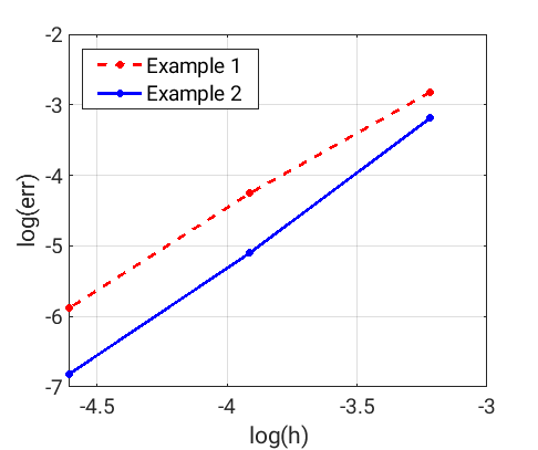
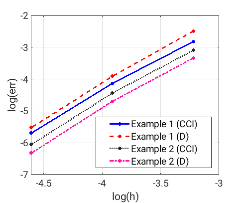
(a)	(b)
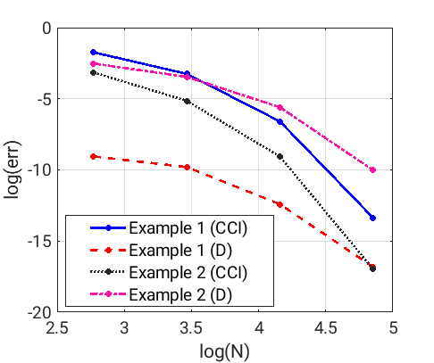
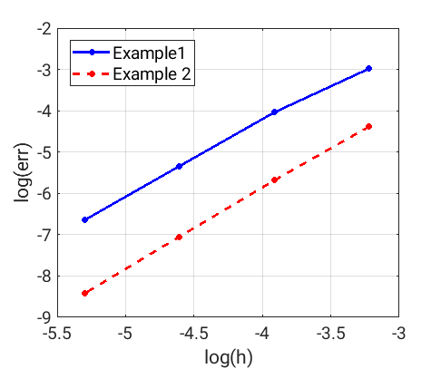
(c)	(d)

Figure 6: Convergence of exceptional values (a), relative errors depend on $h$ (b) and $N$ (c).

6 Conclusion

In the last section of this paper, we compare the two algorithms. Both methods have second order convergence with respect to the meshsize and converge super algebraically with respect to the number of nodal points on $[0,1]$. The computational complexity is also similar with the same parameters. Both methods need to be computed by two steps. In the first step, the exceptional values and eigenfunctions are computed, where a normalization process is needed for the decomposition method. Note that, the computation of the normalization is so small that it can be omitted, since $m_{j}$ is always a very small number. In the second step, we need to solve the linear system (25) for the CCI method, and (36) for the decomposition method. Both matrices are of the same type and size, so the computational complexities and time are also similar.

Both methods also have their advantages and disadvantages. The CCI method requires the additional Assumption 6 which is not necessary for the LAP process and the decomposition method. Fortunately this only excludes a discrete subset of $(0,+\infty)$. The propagating modes are not obtained from the CCI method. But for the CCI method, we don’t need very accurate approximations for the exceptional values. On the other hand, the decomposition method needs good approximations for the exceptional values, but it does not need Assumption 6 and the propagating modes are also computed directly. Moreover, due to the corners on the contour in Figure 5, the error from the complex contour discretization is expected to be larger than the decomposition method for the same $N$. Since both algorithms converge super-algebraically with respect to the parameter $N$, they are very efficient and we can choose either algorithm according to different settings and requirements.

Appendix

6.1 Smooth and analytic functions in Banach spaces

First we recall definitions of smooth and analytic functions with values in Banach spaces.

Definition 18.

Suppose $F$ is a map from an open set $U\subset\mathbb{C}^{N}$ into a complex Banach space $X$. Then

• $F$ is analytic at $z_{0}\in U$ if there is an $R>0$ and a series $\{f_{n}:\,n\in\mathbb{N}\}\subset X$ such that

  $$F(z)=\sum_{n=0}^{\infty}\frac{(z-z_{0})^{n}}{n!}f_{n}$$

  converges uniformly for $z\in B(z_{0},R)\cap U$ where $B(z_{0},R)$ is the disk with center $z_{0}$ and radius $R$.

• $F$ is smooth at $z_{0}\in U$ if its Fréchet derivative exists for any order.

With Definition 18, we can easily define spaces $C^{\omega}([a,b];H^{s}(\Omega_{0}))$, $C^{\infty}([a,b];H^{s}(\Omega_{0}))$ where the functions depend analytically or smoothly on the first variable. The space $C^{\infty}_{per}([a,b];H^{s}(\Omega_{0}))$ is the subspace of $C^{\infty}([a,b];H^{s}(\Omega_{0}))$ with an additional periodic condition on the first variable.

We introduce the Floquet-Bloch transform. For a function $\varphi\in C_{0}^{\infty}(\Omega)$, define the transform

$$(\mathcal{J}\varphi)(\alpha,x):=(2\pi)^{-1/2}\sum_{j\in\mathbb{Z}}\varphi\left(x+\left(\begin{matrix}j\\ 0\end{matrix}\right)\right)e^{-\mathrm{i}\alpha(x_{1}+j)}.$$

It is easily checked that with fixed $\alpha\in\mathbb{R}$, $(\mathcal{J}\varphi)(\alpha,\cdot)$ is $1$-periodic in $x_{1}$-direction. For fixed $x\in\Omega_{0}$, $e^{\mathrm{i}\alpha x_{1}}(\mathcal{J}\varphi)(\alpha,x)$ is $2\pi$-periodic in $\alpha$. The properties of the transform are recalled in the following theorem. For details we refer to [23, 27].

Theorem 19.

The Floquet-Bloch transform is extended to an isometry between $H^{s}(\Omega)$ and $L^{2}((-\pi,\pi);H^{s}_{per}(\Omega_{0}))$ for any $s\in\mathbb{R}$ and its inverse transform is:

$$\left(\mathcal{J}^{-1}\psi\right)(x)=\frac{1}{2\pi}\int_{-\pi}^{\pi}\psi(\alpha,x)e^{\mathrm{i}\alpha x_{1}}\,\mathrm{d}\alpha\,.$$

Moreover, the adjoint operator of $\mathcal{J}$ with respect to the inner product of $L^{2}((-\pi,\pi);L^{2}(\Omega_{0}))$, denoted by $\mathcal{J}^{*}$, equals to $\mathcal{J}^{-1}$.
$\mathcal{J}\varphi$ depends analytically on $\alpha$ if and only if $\varphi$ decays exponentially when $|x_{1}|\rightarrow\infty$.
Note here the subscript ${per}$ is to indicate that the function is periodic with respect to $x_{1}$.

6.2 Normalization of the eigensystem

In this subsection, the Assumption 15 no longer holds. Then by solving (29), we find all eigenvalues and eigenfunctions

$$\left\{\left(\widehat{\beta}_{j}^{h},\widetilde{\varphi}_{\ell,j}^{h}\right):\,j\in J^{h},\,\ell=1,2,\dots,m_{j}\right\},$$

where $m_{j}$ is a positive integer. Then we normalize the system to get the eigenfunction $\widehat{\varphi}^{h}_{\ell,j}$ such that it satisfies (12) and (13). The eigenfunctions are of the form

$$\widehat{\varphi}_{\ell,j}^{h}(x)=\sum_{\ell^{\prime}=1}^{m_{j}}c_{\ell,\ell^{\prime}}^{j}\,\widetilde{\varphi}_{\ell^{\prime},j}^{h}(x)$$ (42)

where the coefficients $c_{\ell,\ell^{\prime}}^{j}\in\mathbb{C}$. Thus the problem is then to find out the approximated eigenvalues $\lambda_{\ell,j}^{h}$ and coefficients $c^{j,h}_{\ell,\ell^{\prime}}$ for all $\ell,\ell^{\prime}=1,2,\dots,m_{j}$. From (12), for fixed $\ell=1,2,\dots,m_{j}$,

$$\sum_{\ell^{\prime}=1}^{m_{j}}c^{j,h}_{\ell,\ell^{\prime}}\left(\int_{\Omega_{0}}\left[-\mathrm{i}\frac{\partial}{\partial x_{1}}\widetilde{\varphi}_{\ell^{\prime},j}^{h}+\widehat{\beta}_{j}\widetilde{\varphi}_{\ell^{\prime},j}^{h}\right]\right)\overline{\widetilde{\varphi}_{\ell^{\prime\prime},j}^{h}}\,\mathrm{d}x\,=\lambda^{h}_{\ell,j}\sum_{\ell^{\prime}=1}^{m_{j}}c^{j,h}_{\ell,\ell^{\prime}}\left(k\int_{\Omega_{0}}\widetilde{\varphi}_{\ell^{\prime},j}^{h}\overline{\widetilde{\varphi}_{\ell^{\prime\prime},j}^{h}}\,\mathrm{d}x\,\right)$$

holds for any $\ell^{\prime\prime}=1,2,\dots,m_{j}$. Let

$$a^{j}_{\ell,\ell^{\prime}}=\int_{\Omega_{0}}\left[-\mathrm{i}\frac{\partial}{\partial x_{1}}\widetilde{\varphi}_{\ell^{\prime},j}^{h}+\widehat{\beta}_{j}\widetilde{\varphi}_{\ell^{\prime},j}^{h}\right]\overline{\widetilde{\varphi}_{\ell,j}^{h}}\,\mathrm{d}x\,;\quad b^{j}_{\ell,\ell^{\prime}}=k\int_{\Omega_{0}}\widetilde{\varphi}_{\ell^{\prime},j}^{h}\overline{\widetilde{\varphi}_{\ell,j}^{h}}\,\mathrm{d}x\,,$$

then

$$\left(\begin{matrix}a^{j}_{1,1}&a^{j}_{1,2}&\cdots&a^{j}_{1,m_{j}}\\ a^{j}_{2,1}&a^{j}_{2,2}&\cdots&a^{j}_{2,m_{j}}\\ \vdots&\vdots&\cdots&\vdots\\ a^{j}_{m_{j},1}&a^{j}_{m_{j},2}&\cdots&a^{j}_{m_{j},m_{j}}\end{matrix}\right)\left(\begin{matrix}c^{j,h}_{\ell,1}\\ c^{j,h}_{\ell,2}\\ \vdots\\ c^{j,h}_{\ell,m_{j}}\end{matrix}\right)=\lambda^{h}_{\ell,j}\left(\begin{matrix}b^{j}_{1,1}&b^{j}_{1,2}&\cdots&b^{j}_{1,m_{j}}\\ b^{j}_{2,1}&b^{j}_{2,2}&\cdots&b^{j}_{2,m_{j}}\\ \vdots&\vdots&\cdots&\vdots\\ b^{j}_{m_{j},1}&b^{j}_{m_{j},2}&\cdots&b^{j}_{m_{j},m_{j}}\end{matrix}\right)\left(\begin{matrix}c^{j,h}_{\ell,1}\\ c^{j,h}_{\ell,2}\\ \vdots\\ c^{j,h}_{\ell,m_{j}}\end{matrix}\right).$$

By solving this generalized eigenvalue problem, we get all the coefficients $c^{j,h}_{\ell,\ell^{\prime}}$ and eigenvalues $\lambda^{h}_{\ell,j}$. Then the function $\widehat{\varphi}^{h}_{\ell,j}$ is obtained directly by (42). Finally, we normalize the functions $\widehat{\varphi}^{h}_{\ell,j}$ by

$$2k\int_{\Omega_{0}}n(x)\widehat{\varphi}^{h}_{\ell,j}(x)\overline{\widehat{\varphi}^{h}_{\ell,j}(x)}\,\mathrm{d}x\,=1.$$

References

- [1] A. Bermudez, R. G. Duran, R. Rodriguez, and J. Solomin. Finite element analysis of a quadratic eigenvalue problem arising in dissipative acoustics. SIAM Journal on Numerical Analysis, 38(1):267–291, 2000.
- [2] D. L. Colton and R. Kress. Integral equation methods in scattering theory. Krieger, repr. ed., with corr. edition, 1992.
- [3] T. Dohnal and B. Schweizer. A bloch wave numerical scheme for scattering problems in periodic wave-guides. SIAM J. Numer. Anal., 56(3):1848–1870, 2018.
- [4] W. Dörfler, A. Lechleite, M. Plum, G. Schneider, and C. Wieners. Photonic crystals: Mathematical analysis and numerical approximation, 2011.
- [5] M. Ehrhardt, H. Han, and C. Zheng. Numerical simulation of waves in periodic structures. Commun. Comput. Phys., 5:849–870, 2009.
- [6] M. Ehrhardt, J. Sun, and C. Zheng. Evaluation of scattering operators for semi-infinite periodic arrays. Commun. Math. Sci., 7:347–364, 2009.
- [7] C. Engström. Spectral approximation of quadratic operator polynomials arising in photonic band structure calculations. Numer. Math., 126:413–440, 2014.
- [8] S. Fliss. Analyse mathématique et numérique de problèmes de propagation des ondes dans des milieux périodiques infinis localement perturbés. PhD thesis, Ecole Polytechnique, 2009.
- [9] S. Fliss. A dirichlet-to-neumann approach for the exact computation of guided modes in photonic crystal waveguides. SIAM Journal on Scientific Computing, 35(2):B438–B461, 2013.
- [10] S. Fliss and P. Joly. Exact boundary conditions for time-harmonic wave propagation in locally perturbed periodic media. Appl. Numer. Math., 59:2155–2178, 2009.
- [11] S. Fliss and P. Joly. Wave propagation in locally perturbed periodic media(case with absorption): Numerical aspects. J. Comput. Phys., 231:1244–1271, 2012.
- [12] S. Fliss and P. Joly. Solutions of the time-harmonic wave equation in periodic waveguides: asymptotic behaviour and radiation condition. Arch. Rational Mech. Anal., 2015.
- [13] G. H. Hardy, J. E. Littlewood, and G. Pólya. Inequalities. Cambridge Mathematical Library. Cambridge University Press, 2nd edition, 1988.
- [14] V. Hoang. The limiting absorption principle for a periodic semin-infinite waveguide. SIAM J. Appl. Math., 71(3):791–810, 2011.
- [15] J.D. Joannopoulos, R.D. Meade, and N. J. Winn. Photonic Crystal-Molding the Flow of Light. Princton University Press, 1995.
- [16] S.G. Johnson and J. D. Joannopoulos. Photonic Crystal - The road from theory to practice. Kluwer Academic Publishers, 2002.
- [17] P. Joly, J.-R. Li, and S. Fliss. Exact boundary conditions for periodic waveguides containing a local perturbation. Commun. Comput. Phys., 1:945–973, 2006.
- [18] A. Kirsch. Scattering by a periodic tube in : part i. the limiting absorption principle. Inverse Problems, 35(10):104004, 2019.
- [19] A. Kirsch. Scattering by a periodic tube in : part ii. the radiation condition. Inverse Problems, 35(10):104005, 2019.
- [20] A. Kirsch and A. Lechleiter. A radiation condition arising from the limiting absorption principle for a closed full‐ or half‐waveguide problem. Math. Meth. Appl. Sci., 41(10):3955–3975, 2018.
- [21] W. G. Kolata. Approximation in variationally posed eigenvalue problems. Numerische Mathematik, 29(2):159–171, 1978.
- [22] R. Kress. Numerical Analysis. Springer, 1998.
- [23] P. Kuchment. Floquet Theory for Partial Differential Equations, volume 60 of Operator Theory. Advances and Applications. Birkhäuser, Basel, 1993.
- [24] P. Kuchment. The mathematics of photonic crystals. In Mathematical modelling in optical science, volume 22 of Frontiers in Applied Mathematics, page Chapter 7, Philadelphia, 2001. SIAM.
- [25] P. Kuchment and B. Ong. On guided waves in photonic crystal waveguides. In P. Kuchment, editor, Waves in Periodic and Random Media, volume 339 of Contemporary Mathematics, pages 105–116. AMS, 2003.
- [26] A. Lechleiter. The Floquet-Bloch transform and scattering from locally perturbed periodic surfaces. J. Math. Anal. Appl., 446(1):605–627, 2017.
- [27] A. Lechleiter and D.-L. Nguyen. Scattering of Herglotz waves from periodic structures and mapping properties of the Bloch transform. Proc. Roy. Soc. Edinburgh Sect. A, 231:1283–1311, 2015.
- [28] A. Lechleiter and R. Zhang. A convergent numerical scheme for scattering of aperiodic waves from periodic surfaces based on the Floquet-Bloch transform. SIAM J. Numer. Anal, 55(2):713–736, 2017.
- [29] A. Lechleiter and R. Zhang. A Floquet-Bloch transform based numerical method for scattering from locally perturbed periodic surfaces. SIAM J. Sci. Comput., 39(5):B819–B839, 2017.
- [30] A. Lechleiter and R. Zhang. Non-periodic acoustic and electromagnetic scattering from periodic structures in 3d. Comput. Math. Appl., 74(11):2723–2738, 2017.
- [31] S. A. Nazarov. Elliptic boundary value problems with periodic coefficients in a cylinder. Math. USSR Izv., 18(1):89–99, 1982.
- [32] S. A. Nazarov. The mandelshtam energy radiation conditions and the umov-poynting vector in elastic waveguides. Probl. Mat. Anal., 72:101–146, 2013.
- [33] S. A. Nazarov. Umov-mandelshtam radiation conditions in elastic periodic waveguides. Sb. Math., 205(7):953–982, 2014.
- [34] S. A. Nazarov and B. A. Plamenevsky. On radiation conditions for selfadjoint elliptic problems. Dokl. Akad. Nauk SSSR, 311(3):532–536, 1990.
- [35] S. A. Nazarov and B. A. Plamenevsky. Radiation principles for selfadjoint elliptic problems. Probl. Mat. Fiz., 13:192–244, 1991.
- [36] S. A. Nazarov and B. A. Plamenevsky. Elliptic Problems in domains with piecewise smooth boundaries, vol 13 of the De Gruyter Expositions in Mathematics. Walter de Gruyter & Co., Berlin, 1994.
- [37] K. Sadoka. Optical Properties of Photonic Crystals. Springer, 2001.
- [38] J. Sun and C. Zheng. Numerical scattering analysis of te plane waves by a metallic diffraction grating with local defects. J. Opt. Soc. Am. A, 26(1):156–162, 2009.
- [39] J.A.C. Weideman. Numerical integration of periodic functions: a few examples. Am. Math. Mon., 109(1):21–35, 2002.
- [40] R. Zhang. A high order numerical method for scattering from locally perturbed periodic surfaces. SIAM J. Sci. Comput., 40(4):A2286–A2314, 2018.
- [41] R. Zhang. Numerical method for scattering problems in periodic waveguides. Numer. Math., 148:959–996, 2021.
- [42] R. Zhang. Spectrum decomposition of translation operators in periodic waveguide. SIAM Journal on Applied Mathematics, 81(1):233–257, 2021.