Monte Carlo Filtering Objectives: A New Family of Variational Objectives to Learn Generative Model and Neural Adaptive Proposal for Time Series

Abstract

Learning generative models and inferring latent trajectories have shown to be challenging for time series due to the intractable marginal likelihoods of flexible generative models. It can be addressed by surrogate objectives for optimization. We propose Monte Carlo filtering objectives (MCFOs), a family of variational objectives for jointly learning parametric generative models and amortized adaptive importance proposals of time series. MCFOs extend the choices of likelihood estimators beyond Sequential Monte Carlo in state-of-the-art objectives, possess important properties revealing the factors for the tightness of objectives, and allow for less biased and variant gradient estimates. We demonstrate that the proposed MCFOs and gradient estimations lead to efficient and stable model learning, and learned generative models well explain data and importance proposals are more sample efficient on various kinds of time series data.

1 Introduction

Learning a generative model with latent variables for time series is of interest in many applications. However, exact inference and marginalization are often intractable for flexible generative models, making it challenging to learn. There are a few popular approaches to circumvent these difficulties: implicit methods that learn generative models by comparing generated samples to data distributions like Generative Adversarial Networks (GANs) (Goodfellow et al., 2014); and explicit methods that define surrogate objectives of the intractable marginal log-likelihood like Variational Autoencoder (VAEs) (Kingma and Welling, 2014), or tractable marginals by invertible transformations like Normalizing Flows (NFs) (Rezende and Mohamed, 2015). Explicit methods are often preferable when latent/encoded information is of importance, e.g. filtering and smoothing problems for some subsequent tasks. In this work, we mainly focus on the second approach and propose a family of surrogate filtering objectives to learn generative models and adaptive importance proposal models for time series.

Researchers have introduced various surrogate objectives using variational approximations of intractable posterior for time series, known as evidence lower bounds (ELBOs), such as STONE (Bayer and Osendorfer, 2014), VRNN (Chung et al., 2015), SRNN (Fraccaro et al., 2016), DKF (Krishnan et al., 2017), KVAE (Fraccaro et al., 2017). However, they typically suffer from a general issue caused by the limited flexibility of the variational approximations, thus restricting the learning of generative models. To alleviate this constraint, IWAE (Burda et al., 2016) proposes a tighter objective by averaging importance weights of multiple samples drawn from a variational approximation. Monte Carlo objectives (MCOs) (Mnih and Rezende, 2016) generalizes the IWAE objective and ELBOs for non-sequential data. AESMC (Le et al., 2018), FIVO (Maddison et al., 2017), and VSMC (Naesseth et al., 2018) extend this idea for sequential data using the estimators by Sequential Monte Carlo (SMC) and propose closely related surrogates objectives for learning.

Inspired by MCOs and the sequential variants, we propose Monte Carlo filtering objectives (MCFOs), a new family of surrogate objectives for generative models of time series, that

• broadens previously limited choices of estimators for time series other than SMC,

• possesses unique properties such as monotonic convergence and asymptotic bias, revealing the factors that determine a tighter objective: the number of samples and importance proposals,

• reduces high variance in gradient estimates of proposal models common in state-of-the-art algorithms, without introducing bias, which allows for faster convergence and sample efficient proposal models.

The paper is organized as follows: we first review the definition of MCOs and discuss common limitations of existing filtering variants. In Section 3, we derive MCFOs, explain their relations to other objectives and important properties. We demonstrate two instances of MCFOs with SMC and Particle Independence Metropolis-Hasting (PIMH) to learn models on 1) Linear Gaussian State Space Models (LGSSMs), 2) nonlinear, non-Gaussian, high dimensional SSMs of video sequences, 3) non-Markovian music sequences.

2 Background

2.1 Monte Carlo Objectives

For a generative model with observation $\mathbf{x}$ and latent state $\mathbf{z}$, a Monte Carlo objective (MCO) (Mnih and Rezende, 2016) is defined as an estimate of the marginal log-likelihood $\log p(\mathbf{x})$ by samples drawn from a proposal distribution $q$:

$$\mathbb{E}_{q(\mathbf{z})}[\log R]=\log p(\mathbf{x})-\mathbb{E}_{q(\mathbf{z})}[\log\frac{p(\mathbf{x})}{R}]\leq\log p(\mathbf{x}),$$ (1)

where $R$ is any unbiased estimator of $p(\mathbf{x})$ that $\mathbb{E}[R]=p(\mathbf{x})$. It is also a lower bound of $\log p(\mathbf{x})$ as can be shown using Jensen’s inequality. When an estimator takes a single sample from $q$ and $R={p(\mathbf{x},\mathbf{z})}/{q(\mathbf{z})}$, the MCO can be identified as ELBO in variational inference (Mnih and Gregor, 2014). When an estimator averages importance weights from $K$ samples, $R^{K}=K^{-1}\sum_{i=1}^{K}{p(\mathbf{z}^{i},\mathbf{x})}/{q(\mathbf{z}^{i})}$, it yields an importance weighted ELBO (IW-ELBO) (Burda et al., 2016; Domke and Sheldon, 2018). This bound is proven to be tighter with increasing $K$ and asymptotically converges to $\log p(\mathbf{x})$, as $K\rightarrow\infty$.

2.2 Sequential Monte Carlo

For a sequential observation $\mathbf{x}_{1:T}$ with latent trajectory $\mathbf{z}_{1:T}$, the generative process can be factorized as $p(\mathbf{z}_{1:T},\mathbf{x}_{1:T})=p(\mathbf{z}_{1})p(\mathbf{x}_{1}|\mathbf{z}_{1})\prod_{t=2}^{T}p(\mathbf{z}_{t}|\mathbf{z}_{1:t-1},\mathbf{x}_{1:t-1})p(\mathbf{x}_{t}|\mathbf{z}_{1:t},\mathbf{x}_{1:t-1})$. Inferring latent trajectory, $p(\mathbf{z}_{1:T}|\mathbf{x}_{1:T})$, is of importance for marginalization and learning of generative models, however, it is usually intractable.

Sequential Monte Carlo (SMC) (Doucet and Johansen, 2009) approximates a target distribution, specifically $p(\mathbf{z}_{1:T}|\mathbf{x}_{1:T})$, using a set of weighted sample trajectories $\{\tilde{w}_{T}^{i},\hat{\mathbf{z}}_{1:T}^{i}\}_{i=1:K}$. It combines Sequential Importance Sampling (SIS) with resampling, and consists of four main steps:

• Sample $K$ particles $\hat{\mathbf{z}}^{i}_{t}$ from proposal $q(\mathbf{z}_{t}|\bar{\mathbf{z}}^{i}_{1:t-1},\mathbf{x}_{1:t})$ with previously resampled trajectories $\bar{\mathbf{z}}^{i}_{1:t-1}$;

• Append to trajectory $\hat{\mathbf{z}}^{i}_{1:t}=(\hat{\mathbf{z}}^{i}_{t},\bar{\mathbf{z}}^{i}_{1:t-1})$;

• Weight trajectories with $\tilde{w}_{t}^{i}={w_{t}^{i}}/{\sum_{j=1}^{K}w_{t}^{j}}$, where
  $w_{t}^{i}={p(\mathbf{x}_{1:t},\hat{\mathbf{z}}_{1:t}^{i}|\mathbf{x}_{1:t-1},\bar{\mathbf{z}}^{i}_{1:t-1})}/{q(\hat{\mathbf{z}}^{i}_{t}|\bar{\mathbf{z}}^{i}_{1:t-1},\mathbf{x}_{1:t})}$;

• Resample from $\{\tilde{w}_{t}^{i},\hat{\mathbf{z}}_{1:t}^{i}\}$ to obtain equally-weighted particles $\bar{\mathbf{z}}^{i}_{1:t}=\hat{\mathbf{z}}_{1:t}^{A_{t-1}^{i}}$, with ancestral indices $A^{i}_{t-1}$.

This iteration continues until time $T$. Besides being an approximate inference, SMC also gives an unbiased estimate of the marginal likelihood $p(\mathbf{x}_{1:T})$ by the importance weights:

$$\hat{p}(\mathbf{x}_{1:T})=\prod_{t=1}^{T}\left(\frac{1}{K}\sum_{i=1}^{K}w_{t}^{i}\right).$$ (2)

The variance of this estimate, accessed by the so-called Effective Sample Size (ESS) for sample efficiency, is largely dependent on the proposal distributions $q$. We refer to (Doucet and Johansen, 2009) for a more in-depth discussion.

2.3 Variational Filtering Objectives

To learn a generative model for time series data, various ELBO-like surrogate objectives have been proposed using different factorizations of generative models and approximations $q(\mathbf{z}_{1:T}|\mathbf{x}_{1:T})$. IW-ELBO can be extended to sequences by changing from Importance Sampling (IS) to SIS estimator $R^{K}=K^{-1}\sum_{i=1}^{K}{p(\mathbf{z}_{1:T}^{i},\mathbf{x}_{1:T})}/{q(\mathbf{z}_{1:T}^{i})}$. However, such an estimator suffers from exponential growth of variance with the length of sequences.To improve this, AESMC, FIVO and VSMC propose three closely related MCOs, exploiting the SMC estimators (2):

$$\text{ELBO}_{\text{SMC}}=\mathbb{E}_{Q_{\text{SMC}}}\bigg{[}\sum_{t=1}^{T}\log\underbrace{\left(\frac{1}{K}\sum_{i=1}^{K}w_{t}^{i}\right)}_{R_{t}^{K}}\bigg{]}$$ (3)

$$Q_{\text{SMC}}(z_{1:T}^{1:K})=\int\left(\prod_{i=1}^{K}q(z_{1}^{i})\right)$$

$$\quad\quad\quad\quad\prod_{t=2}^{T}\prod_{i=1}^{K}\left(q(z_{t}^{i}|z_{1:t-1}^{A_{t-1}^{i}})\cdot\frac{w_{t-1}^{A_{t-1}^{i}}}{\sum_{j}w_{t-1}^{j}}\right)dA_{1:T-1}^{1:K}.$$

It is found that the learning of generative models via the objective suffers high variance in gradient estimation, since importance weight $w_{t}^{i}$ does not allow for smooth gradient computation. We show that simply ignoring some high variance term in the gradient estimate as the suggested solution in previous methods, introduces an extra bias and leads to non-optimality of proposal and generative parameters at convergence. To tackle these problems and extend variational filtering objectives, we propose MCFOs, and discuss their important properties in the following sections.

3 Monte Carlo Filtering Objectives

Instead of constructing variational lower bound from (2), we leverage the following decomposition of joint marginal log-likelihood:

$$\log p(\mathbf{x}_{1:T})=\log p(\mathbf{x}_{1})+\sum_{t=2}^{T}\log p(\mathbf{x}_{t}|\mathbf{x}_{1:t-1}).$$ (4)

Nonetheless, $\log p(\mathbf{x}_{t}|\mathbf{x}_{1:t-1})$ is usually intractable, which makes learning a generative model by maximizing (4) only possible in some limited cases. Instead, we define $\mathcal{L}_{t}^{K}$, an MCO to $\log p(\mathbf{x}_{t}|\mathbf{x}_{1:t-1})$ with $K$ samples:

$$\mathcal{L}_{t}^{K}=\mathbb{E}_{Q_{t}^{K}}[\log R_{t}^{K}],$$ (5)

$$Q_{t}^{K}(\mathbf{z}_{1:t}^{1:K}|\mathbf{x}_{1:t})=p(\mathbf{z}_{1:t-1}^{1:K}|\mathbf{x}_{1:t-1})\cdot\prod_{i=1}^{K}q(\mathbf{z}_{t}^{i}|\mathbf{z}_{1:t-1}^{i},\mathbf{x}_{1:t}),$$

$$R_{t}^{K}=\frac{1}{K}\sum_{i=1}^{K}\frac{p(\mathbf{z}_{1:t}^{i},\mathbf{x}_{1:t})}{p(\mathbf{z}_{1:t-1}^{i},\mathbf{x}_{1:t-1})q(\mathbf{z}_{t}^{i}|\mathbf{z}_{1:t-1}^{i},\mathbf{x}_{1:t})},$$

specifically $$\mathcal{L}_{1}^{K} \log p(\mathbf{x}_{1})$$ for ,

$$Q_{1}^{K}(\mathbf{z}_{1}^{1:K}|\mathbf{x}_{1})=\prod_{i=1}^{K}q(\mathbf{z}_{1}^{i}|\mathbf{x}_{1}),~{}~{}R_{1}^{K}=\frac{1}{K}\sum_{i=1}^{K}\frac{p(\mathbf{z}_{1}^{i},\mathbf{x}_{1})}{q(\mathbf{z}_{1}^{i}|\mathbf{x}_{1})},$$

where $q(\mathbf{z}_{t}|\mathbf{z}_{1:t-1},\mathbf{x}_{1:t})$ and $q(\mathbf{z}_{1}|\mathbf{x}_{1})$ are the proposal distributions, $R_{t}^{K}$ and $R_{1}^{K}$ are the unbiased estimators of $p(\mathbf{x}_{t}|\mathbf{x}_{1:t-1})$ and $p(\mathbf{x}_{1})$ using $K$ samples; see Appendix B.1 for derivations. Summing up the series of MCOs in (5), we then define a Monte Carlo filtering objective (MCFO), $\mathcal{L}_{\text{MCFO}}$:

$$\mathcal{L}_{\text{MCFO}}^{K}(\mathbf{x}_{1:T},p,q)=\sum_{t=1}^{T}\mathcal{L}_{t}^{K}\leq\log p(\mathbf{x}_{1:T}),$$

as the lower bound of $\log p(\mathbf{x}_{1:T})$. To avoid notation clutter, we leave out arguments on $\mathcal{L}_{\text{MCFO}}^{K}$ and $Q_{t}^{K}$ whenever the context permits.

Considering the filtering problem for which future observations have no impact on the current posterior, replacing $p(\mathbf{z}_{1:t-1}^{1:K}|\mathbf{x}_{1:t-1})$ in $Q_{t}^{K}$ with $K$ sample approximations $\hat{p}(\mathbf{z}_{1:t-1}^{1:K}|\mathbf{x}_{1:t-1})=\sum_{i=1}^{K}\tilde{w}_{t-1}^{i}\delta(\mathbf{z}_{1:t-1}^{i}-\hat{\mathbf{z}}_{1:t-1}^{i})$ retrieves the definition of $\text{ELBO}_{\text{SMC}}$ in (3). The objective can be considered as an estimate of MCFOs by SMC and is consistent to MCFOs with the asymptotic bias of $\mathcal{O}(1/K)$; see Appendix B.2 for detailed discussion. MCFOs can freely choose other estimator alternatives such as PIMH (Andrieu et al., 2010) and unbiased MCMC with couplings (Jacob et al., 2017) to further improve sampling efficiency of SMC.

3.1 Properties of MCFOs

Except for the general properties inherited from MCOs such as bound and consistency, the convergence of MCFOs is monotonic like IW-ELBO, but unique to earlier filtering objectives. Additionally, the asymptotic bias of MCFOs can be shown to relate to the total variances of estimators.

Proposition 1.

(Properties of MCFOs). Let $\mathcal{L}_{\text{MCFO}}^{K}$ be an MCFO of $\log p(\mathbf{x}_{1:T})$ by a series of unbiased estimators $R_{t}$ of $p(\mathbf{x}_{t}|\mathbf{x}_{1:t-1})$ using $K$ samples. Then,

1. (Bound) $\log p(\mathbf{x}_{1:T})\geq\mathcal{L}_{\text{MCFO}}^{K}$.

2. (Monotonic convergence) $\mathcal{L}_{\text{MCFO}}^{K+1}\geq\mathcal{L}_{\text{MCFO}}^{K}\geq\ldots\geq\mathcal{L}_{\text{MCFO}}^{1}$.

3. (Consistency) If $p(\mathbf{z}_{1},\mathbf{x}_{1})/q(\mathbf{z}_{1}|\mathbf{x}_{1})$ and ${p(\mathbf{z}_{1:t},\mathbf{x}_{1:t})}/{(p(\mathbf{z}_{1:t-1},\mathbf{x}_{1:t-1})q(\mathbf{z}_{t}|\mathbf{z}_{1:t-1},\mathbf{x}_{1:t}))}$ for all $t\in[2,T]$ are bounded, then $\mathcal{L}_{\text{MCFO}}^{K}\rightarrow\log p(\mathbf{x}_{1:T})$ as K $\rightarrow\infty$.

4. (Asymptotic Bias) For a large K, the bias of bound is related to the variance of estimator $R_{t}$, $\mathbb{V}[R_{t}]$,

   $$\lim_{K\rightarrow\infty}K(\log p(\mathbf{x}_{1:T})-\mathcal{L}_{\text{MCFO}}^{K})=\sum_{t=1}^{T}\frac{\mathbb{V}[R_{t}]}{2p(\mathbf{x}_{t}|\mathbf{x}_{1:t-1})^{2}}.$$

Proof.

See Appendix B.3.

Although increasing the number of samples $K$ leads to a tighter MCFO, a too large $K$ is infeasible in terms of computational and memory. It has also been shown that larger $K$ may deteriorate to learn proposals (Rainforth et al., 2018). An appropriate $K$ is a critical hyperparameters that affects learning and inference. On the other hand, asymptotic bias suggests another way for a tighter bound, i.e. using less variant estimators $R_{t}$, which is something that has been overlooked in recent literature. It explains why the bounds defined by SMC are tighter than IW-ELBO by SIS. Thus, a proposal model that permits less variant $R_{t}$, either designed or learned, is another key instrument.

3.2 Optimal Importance Proposals

Considering proposals $q$ as an argument of MCFOs, we can derive the optimal proposals when they maximize the bound.

Proposition 2.

(Optimal importance proposals $q^{*}$ for an MCFO). The bound is maximized and exact to $\log p(\mathbf{x}_{1:T})$ when the importance proposals are

$$q^{*}(\mathbf{z}_{1}|\mathbf{x}_{1})=p(\mathbf{z}_{1}|\mathbf{x}_{1}),$$

$$\text{for all }t=2:T$$

$$q^{*}(\mathbf{z}_{t}|\mathbf{z}_{1:t-1},\mathbf{x}_{1:t})=\frac{p(\mathbf{z}_{1:t}|\mathbf{x}_{1:t})}{p(\mathbf{z}_{1:t-1}|\mathbf{x}_{1:t-1})}=p(\mathbf{z}_{t}|\mathbf{z}_{1:t-1},\mathbf{x}_{1:t}).$$

Proof.

See Appendix B.4.

The optimal importance proposals always propagate samples from the previous filtering posterior $p(\mathbf{z}_{1:t-1}|\mathbf{x}_{1:t-1})$ to the new target $p(\mathbf{z}_{1:t}|\mathbf{x}_{1:t})$, thus leads MCFOs to be exact. For SSMs that assume Markovian latent variables and conditional independent observations, the optimal importance proposals are further simplified to $p(\mathbf{z}_{t}|\mathbf{z}_{t-1},\mathbf{x}_{t})$ (Doucet et al., 2000, Proposition 2). For common intractable problems, though the filtering posteriors and optimal proposals are not accessible, we can learn a parametric adaptive importance proposal model jointly with generative models by optimizing MCFOs.

3.3 Learning Generative and Proposal Models

Method	$\triangledown_{\boldsymbol{\phi}}$	$\triangledown_{\boldsymbol{\theta}}$
MCFO	See (7)	See (8)
AESMC/FIVO/VSMC	$$\triangledown_{\boldsymbol{\theta},\boldsymbol{\phi}}\log\hat{p}(\mathbf{x}_{1:T})+\sum_{t=2}^{T}\log\frac{\hat{p}(\mathbf{x}_{1:t})}{\hat{p}(\mathbf{x}_{1:t-1})}\left(\sum_{i=1}^{K}\triangledown_{\boldsymbol{\theta},\boldsymbol{\phi}}\log({w_{t-1}^{A_{t-1}^{i}}}/{\sum_{j}w_{t-1}^{j}})\right)$$ (6)
IWAE	$\triangledown_{\boldsymbol{\theta},\boldsymbol{\phi}}f_{\boldsymbol{\theta},\boldsymbol{\phi}}(\mathbf{x}_{1:T},\tilde{g}_{\boldsymbol{\phi}}(\mathbf{x}_{1:T}^{1},\boldsymbol{\epsilon}_{1:T}^{1}),\ldots,\tilde{g}_{\boldsymbol{\phi}}(\mathbf{x}_{1:T},\boldsymbol{\epsilon}_{1:T}^{K}))$, where $\tilde{g}$ is reparameterized function of $q_{\boldsymbol{\phi}}(\mathbf{z}_{1:T}|\mathbf{x}_{1:T})$
NASMC	$\sum_{t=1}^{T}\sum_{i=1}^{K}\tilde{w}_{t}^{i}\triangledown_{\boldsymbol{\phi}}\log q_{\boldsymbol{\phi}}(\hat{\mathbf{z}}_{t}^{i}|\mathbf{x}_{1:t},\hat{\mathbf{z}}_{1:t-1}^{A_{t-1}^{i}})$	$\sum_{t=1}^{T}\sum_{i=1}^{K}\tilde{w}_{t}^{i}\triangledown_{\boldsymbol{\theta}}\log p_{\boldsymbol{\theta}}(\hat{\mathbf{z}}_{t}^{i},\mathbf{x}_{t}|\mathbf{x}_{1:t-1},\hat{\mathbf{z}}_{1:t-1}^{A_{t-1}^{i}})$

Table 1: Comparison of gradient estimates by MCFO, AESMC/FIVO/VSMC, IWAE, NASMC.

To illustrate the learning of a flexible importance proposal and/or a generative model, we explicitly parameterize generative model $p_{\boldsymbol{\theta}}$ and proposal model $q_{\boldsymbol{\phi}}$ by $\boldsymbol{\theta}$ and $\boldsymbol{\phi}$ respectively, and optimize them by gradient-based algorithms.

Earlier methods suffer from high variance in gradient estimate due to the second term in (6) in Table 1. This is mainly caused by 1) large magnitudes of $\log\hat{p}(\mathbf{x}_{1:T})$, especially at the beginning of training (Mnih and Gregor, 2014); and 2) high variance in the gradient for non-smooth categorical distribution of discrete ancestral indices $A_{t-1}^{i}$ in SMC. FIVO and VSMC propose to ignore the high variance term to stabilize and accelerate convergence. However, it comes at the cost of an induced bias that cannot be eliminated by increasing the number of samplesand deteriorates the convergence to optimum (Roeder et al., 2017).

MCFOs circumvent the issue for $\triangledown_{\boldsymbol{\phi}}\mathcal{L}_{\text{MCFO}}^{K}$ by the reparameterization trick (Kingma and Welling, 2014) without an extra bias. Assuming the proposal distribution $q_{\boldsymbol{\phi}}$ is reparameterizable (Mohamed et al., 2020), $\triangledown_{\boldsymbol{\phi}}\mathcal{L}_{t}^{K}$ is estimated less variantly by:

$$\triangledown_{\boldsymbol{\phi}}\mathcal{L}_{t}^{K}=\mathbb{E}_{p_{\boldsymbol{\theta}}(\mathbf{z}_{1:t-1}^{i}|\mathbf{x}_{1:t-1})}\big{[}\triangledown_{\boldsymbol{\phi}}\mathbb{E}_{q_{\boldsymbol{\phi}}(\mathbf{z}_{t}^{i}|\mathbf{z}_{1:t-1}^{i},\mathbf{x}_{1:t})}$$ (7)

$$\quad\left(\log\frac{1}{K}\sum_{i=1}^{K}\frac{p_{\boldsymbol{\theta}}(\mathbf{z}_{1:t}^{i},\mathbf{x}_{1:t})}{p_{\boldsymbol{\theta}}(\mathbf{z}_{1:t-1}^{i},\mathbf{x}_{1:t-1})q_{\boldsymbol{\phi}}(\mathbf{z}_{t}^{i}|\mathbf{z}_{1:t-1}^{i},\mathbf{x}_{1:t})}\right)\big{]}$$

$$\simeq \triangledown_{\boldsymbol{\phi}}f_{\boldsymbol{\theta},\boldsymbol{\phi}}(\mathbf{x}_{1:t},\hat{\mathbf{z}}_{1:t-1}^{1:K},$$

$$\quad\underbrace{g_{\boldsymbol{\phi}}(\hat{\mathbf{z}}_{1:t-1}^{1},\boldsymbol{\epsilon}^{i},\mathbf{x}_{1:t}),\ldots,g_{\boldsymbol{\phi}}(\hat{\mathbf{z}}_{1:t-1}^{K},\boldsymbol{\epsilon}^{K},\mathbf{x}_{1:t})}_{\text{reparameterization trick, }\hat{\mathbf{z}}_{t}^{i}=g_{\boldsymbol{\phi}}(\hat{\mathbf{z}}_{1:t-1}^{i},\boldsymbol{\epsilon}^{i},\mathbf{x}_{1:t})}),$$

where $\{\hat{\mathbf{z}}_{1:t}^{i}\}_{i=1:K}$ are K sample trajectories, e.g. from SMC, and can be specified with ancestral indices $A_{t-1}^{i}$ when resampling applies, $f_{\boldsymbol{\theta},\boldsymbol{\phi}}(\cdot)$ is the logarithm average function $\log\frac{1}{K}\sum_{i=1}^{K}\left(\frac{\cdot}{\cdot}\right)$, and $\boldsymbol{\epsilon}^{i}$ is a sample from a base distribution $p(\boldsymbol{\epsilon})$. The same trick cannot directly apply to $\triangledown_{\boldsymbol{\theta}}\mathcal{L}_{t}^{K}$, because of the existence of $\boldsymbol{\theta}$ in the expectation. Instead, we use the score function of $p(\mathbf{x}_{t}|\mathbf{x}_{1:t-1})$ to estimate $\triangledown_{\boldsymbol{\theta}}\mathcal{L}_{t}^{K}$:

$$\triangledown_{\boldsymbol{\theta}}\mathcal{L}_{t}^{K}\simeq\sum_{i=1}^{K}\tilde{w}^{i}_{t}\triangledown_{\boldsymbol{\theta}}\log p_{\boldsymbol{\theta}}(\mathbf{x}_{t},\hat{\mathbf{z}}_{t}^{i}|\mathbf{x}_{1:t-1},\hat{\mathbf{z}}_{1:t-1}^{i}),$$ (8)

where $\tilde{w}^{i}_{t}$ are the normalized importance weights of $\hat{\mathbf{z}}_{1:t}^{i}$; see Appendix B.5 and B.6 for detailed derivation of (7) and (8). Essentially, the score function estimate is equivalent as dropping the high variance term in (6) for $\triangledown_{\boldsymbol{\theta}}$.

NASMC (Gu et al., 2015) is closely related to MCFOs with SMC implementation in terms of $\triangledown_{\boldsymbol{\theta}}$, and RWS (Bornschein and Bengio, 2015) is a special case of NASMC that replaces SMC by SIS. These two methods, however, construct a different surrogate objectives for optimizing $\boldsymbol{\phi}$. While NASMC and RWS minimize the approximated inclusive KL-divergence, $\text{KL}(\hat{p}_{\boldsymbol{\theta}}(\mathbf{z}_{1:t}|\mathbf{x}_{1:t})||q_{\boldsymbol{\phi}}(\mathbf{z}_{1:t}|\mathbf{x}_{1:t}))$, MCFOs minimize the disclusive KL-divergence, $\text{KL}(Q_{t}^{K}(\mathbf{z}_{1:t}^{1:K}|\mathbf{x}_{1:t})||p_{\boldsymbol{\theta}}(\mathbf{z}_{1:t}^{1:K}|\mathbf{x}_{1:t}))$, on the extended latent space as the dual problem of maximizing surrogate objectives. When the family of proposals is adequately flexible to include simple true posteriors, both NASMC and MCFOs converge to the same optimum. To fit a potentially complex multi-modal posterior, the simple proposal learned by NASMC and RWS tends to have undesired low density everywhere in order to cover all modalities, thus impairs the sample efficiency of estimators and restricts the learning of generative models. For MCFOs, $Q_{t}^{K}(\mathbf{z}_{1:t}^{1:K}|\mathbf{x}_{1:t})$ is naturally a mixture of simple proposal distributions $q_{\phi}$ with importance weights $\tilde{w}_{t-1}^{i}$, which remains flexible to fit multi-modal posteriors, while sustaining sample efficiency.

Furthermore, when the latent and observation variables of generative models are assumed to be finite-order Markovian, both gradients of MCFOs can be updated in an incremental manner which makes them well suited for arbitrarily long sequences and data streams.

4 Experiments

We seek to evaluate our method in experiments by answering: 1) what is the side-effect of ignoring the high variance term as proposed in earlier methods; 2) do the gradient estimates of MCFOs reduce the variance without the cost of additional bias; 3) how does the number of samples affect the learning of generative models and how sample efficient are the learned proposal models? We evaluate two instances of MCFOs, MCFO-SMC and MCFO-PIMH, using SMC and PIMH respectively to learn generative and proposal models on LGSSM, non-Gaussian, nonlinear, high dimensional SSMs of video sequences, and non-Markovian polyphonic music sequences. We restrict the form of posteriors to $q_{\boldsymbol{\phi}}(\mathbf{z}_{t}|\mathbf{z}_{t-1},\mathbf{x}_{t})$ for SSM cases to encode history into low dimensional representations, while using VRNN (Chung et al., 2015) to accommodate long temporal dependencies for non-Markovian data. To be noted, all models are amortized over all time instances.

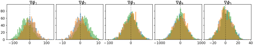
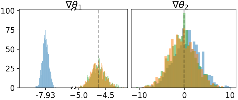
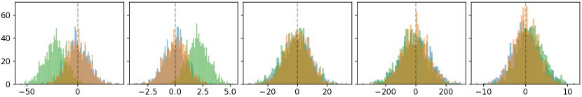
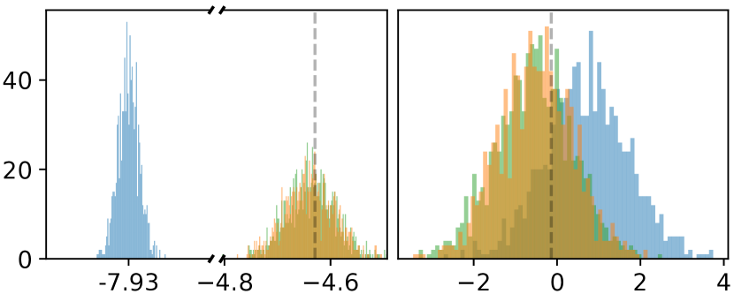
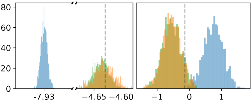
Figure 1: Gradient estimates of IWAE, AESMC, MCFO with respect to generative and proposal parameters at their optima with different numbers of samples $K$; Top: $K=10$, Middle: $K=100$, Bottom: $K=1000$.

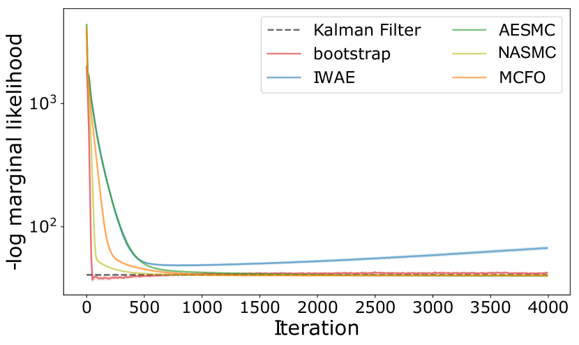
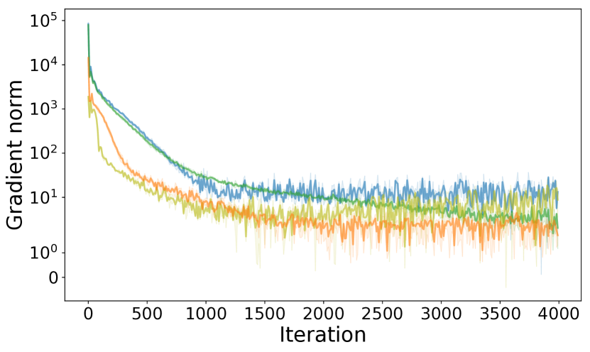
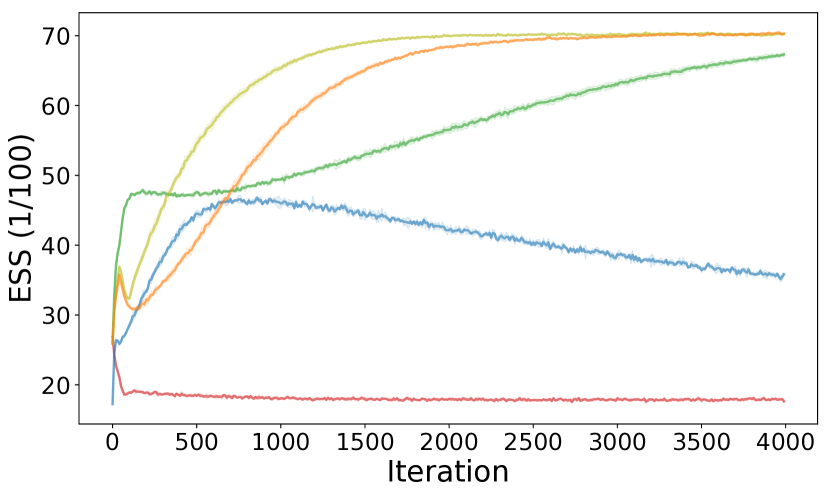
Figure 2: Left: Negative marginal log-likelihoods (NLLs) on test data. Middle: Gradient norms of parameters. Right: Effective sample size (ESS). Lines indicate the average of 3 random seed trainings and shaded areas for standard deviation. See Figure 7 for the convergence of generative and proposal parameters, $\boldsymbol{\theta}$ and $\boldsymbol{\phi}$ in Appendix D.2.

4.1 Gradient Estimation

Following (Rainforth et al., 2018; Le et al., 2018), we carry out experiments to examine gradient estimators on a tractable LGSSM, defined by $\theta_{1}$ and $\theta_{2}$, and importance proposal $q_{\boldsymbol{\phi}}(\mathbf{z}_{t}|\mathbf{z}_{t-1},\mathbf{x}_{t})$, parameterized by $\boldsymbol{\phi}$:

$$p(z_{1})=\mathcal{N}(z_{1};\mu_{0},\sigma_{0}^{2}),p_{\boldsymbol{\theta}}(z_{t}|z_{t-1})=\mathcal{N}(z_{t};\theta_{1}z_{t-1},\Sigma_{Q}),$$ (9)

$$p_{\boldsymbol{\theta}}(x_{t}|z_{t})=\mathcal{N}(x_{t};\theta_{2}z_{t},\Sigma_{R}),$$

$$q_{\boldsymbol{\phi}}(z_{1}|x_{1})=\mathcal{N}(z_{1};\phi_{1}x_{1}+\phi_{2},\Sigma_{q,1}),$$

$$q_{\boldsymbol{\phi}}(z_{t}|z_{t-1},x_{t})=\mathcal{N}(z_{t};\phi_{3}z_{t-1}+\phi_{4}x_{t}+\phi_{5},\Sigma_{q,t}).$$

See Appendix C.1 for detailed derivations.

The gradient estimates are computed by backwards automatic differentiation (Baydin et al., 2017) on the objectives defined by IWAE, AESMC and MCFO-SMC w.r.t. $\boldsymbol{\theta}$ and $\boldsymbol{\phi}$ using sequences generated by the LGSSM. AESMC is implemented ignoring the high variance term in (6) as suggested. Figure 1 shows 1000 gradient samples by all three methods under different numbers of samples, $K$, when both $\boldsymbol{\theta}$ and $\boldsymbol{\phi}$ are at their optima.

For $\triangledown\boldsymbol{\phi}$, the induced bias of AESMC is distinct and does not disappear with increasing $K$, which makes parameters unable to converge to the exact optimum. Although increasing $K$ decreases the variance for all methods, it is specially detrimental to AESMC for which gradient estimates are barely close to true gradients (Rainforth et al., 2018), but beneficial to IWAE and MCFO. For $\triangledown\boldsymbol{\theta}$, MCFO and AESMC have similar estimates close to the analytical gradients, while IWAE estimates are substantially deviated due to the high variance of SIS estimators. Given the empirical gain of an alternating strategy with optimizing IWAE objective for $\boldsymbol{\phi}$ and AESMC for $\boldsymbol{\theta}$ (Le et al., 2018), training by MCFOs is expected to have a similar performance but with less computations. See Appendix D.1 for more gradient estimates at other locations.

4.2 Learning and Inference on LGSSMs

To examine the learning of generative and proposal parameters, we generate 5000 trajectories by LGSSM in (9) with $\theta_{1}=0.9$, $\theta_{2}=1.2$, of which 4000 are for training and rest for testing. Figure 2 illustrates 5 benchmarking methods including bootstrap filtering (Särkkä, 2013), IWAE, AESMC, NASMC and MCFO-SMC, using the same initialization and optimizer; see Appendix D.2 for experiment setups. Note that bootstrap uses prior as proposal, thus no proposal parameter needs to learn. To evaluate the performance of learned proposal models for sample efficiency and tightness of lower bound, we report the variance of estimators by $\text{ESS}=(\sum_{i}(\tilde{w}_{t}^{i})^{2})^{-1}$, and average over test sequences.

MCFO-SMC and NASMC learn more sample efficient proposal models than bootstrap, AESMC and IWAE, and converge to the exact analytic optimum. Although AESMC does not differ significantly in terms of NLLs from MCFO and NASMC, the bias in gradient estimates shown previously, causes it slow to converge and cannot converge to the exact optimum. MCFO learns both generative and proposal models faster than AESMC. For this simple case, NASMC converges faster than MCFOs, since fitting a Gaussian proposal with NASMC to the uni-modal Gaussian posterior of LGSSM is easier than fitting a mixture of Gaussian proposals with MCFO. However, NASMC may fail to learn multi-modal posteriors for general intractable problems, as shown in the next section. Furthermore, increasing the number of samples and replacing SMC by PIMH with different number of sweeps only slightly improve the learning by MCFOs, see more results in Appendix D.2.

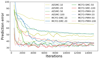
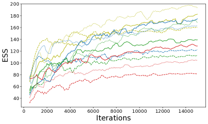
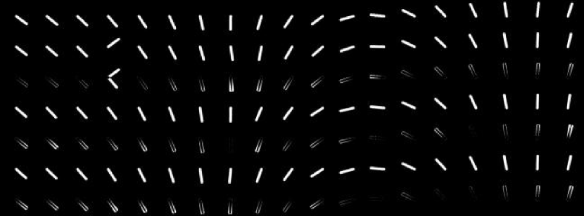
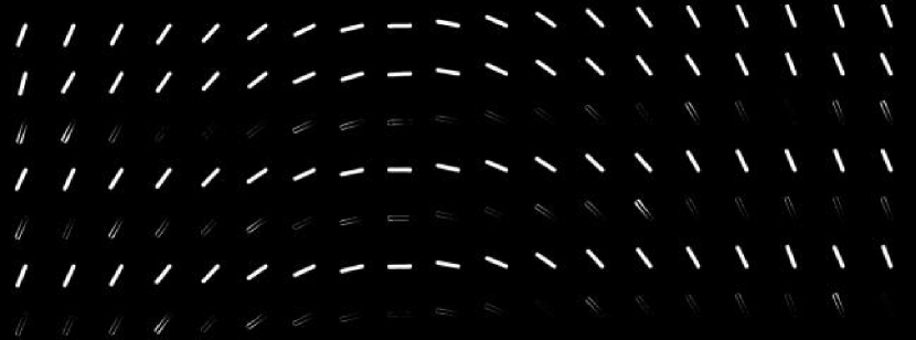
Figure 3: Left, Middle: One-step prediction errors and ESS on the test sets of generative and proposal models learned by AESMC, MCFO-SMC, MCFO-PIMH with $K=10,20,50,100$, evaluated by SMC with 1000 samples and moving average over 3 evaluation runs. Right: Two sequences with one-step predictions by AESMC, MCFO-SMC and MCFO-PIMH with $K=100$. Each row is Bernoulli mean of observations, the one-step predictions and the absolute differences between predictions and observations by AESMC, MCFO-SMC and MCFO-PIMH.

	$K$	AESMC	MCFO-SMC	MCFO-PIMH	$K$	AESMC	MCFO-SMC	MCFO-PIMH
Prediction	10	65.53 $\pm$ 0.18	47.54 $\pm$ 0.94	42.14 $\pm$ 1.49	50	50.84 $\pm$ 0.16	34.06 $\pm$ 1.46	37.01 $\pm$ 1.47
ESS		160.04 $\pm$ 1.97	180.97 $\pm$ 3.16	195.62 $\pm$ 3.05		112.53 $\pm$ 2.42	139.24 $\pm$ 2.46	168.78$\pm$ 4.51
Prediction	20	51.13 $\pm$ 0.37	37.18 $\pm$ 0.72	33.82 $\pm$ 2.06	100	37.87 $\pm$ 0.21	36.17 $\pm$ 1.82	33.71 $\pm$ 0.98
ESS		122.51 $\pm$ 1.89	172.99 $\pm$ 3.46	163.01 $\pm$ 2.10		81.93 $\pm$ 0.82	130.09 $\pm$ 2.12	104.53 $\pm$ 1.94

Table 2: One-step prediction errors and ESS on the test set of generative and proposal models learned by AESMC, MCFO-SMC, MCFO-PIMH with $K=10,20,50,100$, evaluated by SMC with 1000 samples averaged over last 1000 iterations.

Methods	Nottingham	JSB chorales	MuseData	Piano-midi.de
MCFO-SMC-10	2.23 $\pm$0.16	3.87 $\pm$0.09	3.79 $\pm$0.10	6.24$\pm$0.14
MCFO-SMC-20	2.14 $\pm$0.13	3.69 $\pm$0.12	3.65 $\pm$0.11	6.11$\pm$0.15
MCFO-PIMH-10	2.12 $\pm$0.10	3.63 $\pm$0.07	3.59 $\pm$0.08	6.08$\pm$0.09
MCFO-PIMH-20	2.06 $\pm$0.08	3.54 $\pm$0.08	3.48 $\pm$0.10	6.03 $\pm$0.12
FIVO	2.58 $\dagger$ (2.60 $\pm$ 0.18)	4.08 $\dagger$ (3.90 $\pm$0.14)	5.80 $\dagger$ (5.85$\pm$0.15)	6.41 $\dagger$ (6.37$\pm$0.19)
IWAE	2.52 $\dagger$ (2.50 $\pm$ 0.25)	5.77 $\dagger$ (5.43$\pm$0.20)	6.54 $\dagger$ (6.28$\pm$0.23)	6.74 $\dagger$ (6.54$\pm$0.21)
NASMC (Gu et al., 2015) $\dagger$	2.72	3.99	6.89	7.61
SRNN (Fraccaro et al., 2016) $\dagger$	2.94	4.74	6.28	8.20
STONE (Bayer and Osendorfer, 2014) $\dagger$	2.85	6.91	6.16	7.13

Table 3: Estimated NLL per time on polyphonic test sets by SMC with 500 particles. MCFOs, FIVO and IWAE are evaluated by 10 runs, and both FIVO and IWAE, trained the same as MCFO-SMC-10, are reported in parenthesis. $\dagger$ is originally reported in (Maddison et al., 2017).

4.3 Video Sequences

To assess MCFOs in more general cases, we simulate 1000 video sequences of a single pendulum system in gym (Brockman et al., 2016), out of which 500 are used for testing. Each sequence contains 20 $32\times 32$ pixel grayscale images representing factorized Bernoulli distributions of high-dimensional observations; see examples in Figure 3. The transition and proposal distributions, $p_{\boldsymbol{\theta}}(\mathbf{z}_{t}|\mathbf{z}_{t-1})$ and $q_{\boldsymbol{\phi}}(\mathbf{z}_{t}|\mathbf{x}_{t},\mathbf{z}_{t-1})$, are parameteric Gaussian MLPs, while observation models, $p_{\boldsymbol{\theta}}(\mathbf{x}_{t}|\mathbf{z}_{t})$, are parameteric Bernoulli MLPs. The latent dimension is set to 3, and optimizers and model definitions are the same for all methods; see Appendix E for a detailed description of experiment setups.

Figure 3 shows the commonly used one-step prediction errors in observations and ESSs on the test set, evaluated by SMC with 1000 particles on the models trained by AESMC, MCFO-SMC and MCFO-PIMH with $K=10,20,50,100$. Additionally, Table 2 reports both metrics averaged over the last 1000 iterations of trainings. Note that NASMC fails to converge in this task regardless of $K$. Compared to AESMC, both MCFO-SMC and MCFO-PIMH, show quicker convergences, lower prediction errors and higher ESSs that indicate more sample efficient proposal models, especially at smaller $K$. Furthermore, Figure 11 in Appendix E shows that MCFOs implicitly regularize for simpler generative models. Although MCFO-PIMH converges faster than MCFO-SMC and AESMC because of better Monte Carlo approximations, the improvement at convergence is marginally small considering that it requires more computations for each sweep in PIMH. Increasing $K$ does improve generative model learning, but slightly impairs the sample efficiency of proposal models. No statistically significant gain is observed to increase $K$ over 200. Therefore, the sweet spot of $K$ needs to balance the performance of generation and inference.

4.4 Polyphonic Music

To demonstrate the performance of MCFOs for non-Markovian high dimensional data with complex temporal dependencies, we train VRNN models with MCFO-SMC and MCFO-PIMH on four polyphonic music datasets (Boulanger et al., 2012). We preprocess all musical notes to 88-dimensional binary sequences and configure generative and proposal models as in (Maddison et al., 2017); see Appendix F for experiment details. Table 3 reports the estimated NLLs using 500 samples, as with the other benchmarked methods, on the models trained by MCFO-SMC and MCFO-PIMH with 10, 20 samples. As can be seen for all four datasets, MCFO-SMC and MCFO-PIMH are either superior or comparable to the other state-of-the-art algorithms.

5 Conclusion

We introduce Monte Carlo filtering objectives (MCFOs), a new family of variational filtering objectives for learning generative and amortized importance proposal models of time series. MCFOs extend to a wider choice of estimators and accommodate important theoretical properties to achieve tighter objectives. We show empirically that MCFOs and the proposed gradient estimators facilitate more stable and efficient learning on parametric generative and importance proposal models, compared to a number of state-of-the-art methods in various tasks. In future works, we would like to extend MCFOs to smoothing problems and explore tractable MCFOs by flow-based methods.

Appendix

A Sampling Methods of Sequences

A.1 Sequential Monte Carlo

Algorithm 1 Sequential Monte Carlo

0:  observation sequence $\mathbf{x}_{1:T}$, the number of particles $K$, proposal distributions $\{q(\mathbf{z}_{t}|\mathbf{z}_{1:t-1},\mathbf{x}_{1:t})\}_{t=1:T}$, joint likelihoods $\{p(\mathbf{x}_{1:t},\mathbf{z}_{1:t})\}_{t=1:T}$

1:  Sample $\hat{\mathbf{z}}_{1}^{i}$ from $q_{1}(\mathbf{z}_{1})$, for $i=1:K$

2:  Compute weights $w_{1}^{i}=\frac{p(\mathbf{x}_{1},\hat{\mathbf{z}}_{1}^{i})}{q(\hat{\mathbf{z}}_{1}^{i}|\mathbf{x}_{1})}$ and normalize weights $\tilde{w}_{1}^{i}=\frac{w_{1}^{i}}{\sum_{j=1}^{K}w_{1}^{j}}$

3:  Resample $\bar{\mathbf{z}}_{1}^{i}$ from $\{\tilde{w}_{1}^{i},\hat{\mathbf{z}}_{1}^{i}\}$

4:  for $t=2:T$ do

5:     Sample $\hat{\mathbf{z}}_{t}^{i}$ from $q(\mathbf{z}_{t}|\bar{\mathbf{z}}_{1:t-1}^{i},\mathbf{x}_{1:t})$

6:     Set $\hat{\mathbf{z}}^{i}_{1:t}=(\bar{\mathbf{z}}_{1:t-1}^{i},\hat{\mathbf{z}}_{t}^{i})$

7:     Compute weights    $w_{t}^{i}=\frac{p(\mathbf{x}_{1:t},\hat{\mathbf{z}}_{1:t}^{i})}{p(\bar{\mathbf{z}}^{i}_{1:t-1},\mathbf{x}_{1:t-1})q(\hat{\mathbf{z}}^{i}_{t}|\bar{\mathbf{z}}^{i}_{1:t-1},\mathbf{x}_{1:t})}$, and normalize weights $\tilde{w}_{t}^{i}=\frac{w_{t}^{i}}{\sum_{j=1}^{K}w_{t}^{j}}$

8:     Resample $\bar{\mathbf{z}}_{1:t}^{i}=\hat{\mathbf{z}}_{1:t}^{A_{t-1}^{i}}$ from $\{\tilde{w}_{t}^{i},\hat{\mathbf{z}}_{1:t}^{i}\}$, where $A_{t-1}^{i}$ is the anstral index

9:  end for

10:  return  weighted trajectories $\{w_{1:T}^{i},\hat{\mathbf{z}}^{i}_{1:T}\}_{i=1:K}$, marginal likelihood estimates $\hat{p}(\mathbf{x}_{1:T})=\prod_{t=1}^{T}\frac{1}{K}\sum_{i=1}^{K}w_{t}^{i}$

AESMC, VSMC and FIVO, define three closely related MCOs, exploit the estimators by SMC as in (2). The main differences between these objectives lie in their implementations of SMCs: AESMC implements the classic SMC as [Doucet and Johansen, 2009, Section 3.5]; VSMC assumes Markovian latent variables and conditional independence of observation so that proposal models are simplified to the form of $q(\mathbf{z}_{t}|\mathbf{z}_{t-1},\mathbf{x}_{t})$ and observation conditionals to $p(\mathbf{x}_{t}|\mathbf{z}_{t})$ in the generative models; FIVO defines objectives using the adaptive resampling SMC [Doucet and Johansen, 2009, Section 3.5], but it uses a fixed resampling schedule as AESMC during training.

A.2 Particle Independence Metropolis-Hastings

Although resampling in SMC substantially decreases the variance in estimates of marginal likelihoods compared to Sequential Importance Sampling (SIS), the approximations of SMC deteriorate when the sample components are not rejuvenated at subsequent time steps [Andrieu et al., 2010]. To give a more reliable approximation of the posterior, particle independence Metropolis-Hastings (PIMH) [Andrieu et al., 2010] uses SMC approximations as proposal distributions in Metropolis-Hastings (MH) iterations, and compute the acceptance ratio using the estimates of marginal distributions by SMC. Algorithm 2 provides pseudo-code for sampling with PIMH.

To be noted, the PIMH sampler itself might not be a serious competitor to standard SMC and the potential improvement comes along with increased computational cost. Combining with other MCMC transitions e.g. PIMH implemented in particle marginal Metropolis-Hastings is found to better target to the true posterior of latent variables and model parameters. We use PIMH in our experiments as a complement to standard SMC to investigate whether better approximations of posteriors lead to better learning in generative and proposal models. To be noted, the number of SMC sweeps per iteration, $M$, needs to be specified by the user, thus PIMH requires more computations compared to standard SMC.

Algorithm 2 Particle independent Metropolis-Hastings

1:  Run SMC to obtain approximate $\hat{p}(\mathbf{z}_{1:T}|\mathbf{x}_{1:T})$, and sample $\mathbf{z}_{1:T}(0)$ from $\hat{p}(\mathbf{z}_{1:T}|\mathbf{x}_{1:T})$ and compute marginal likelihood estimates $\hat{p}(\mathbf{x}_{1:T})(0)$.

2:  for $m=1:M$ do

3:     run SMC to sample $\mathbf{z}^{*}_{1:T}$ from $\hat{p}(\mathbf{z}_{1:T}|\mathbf{x}_{1:T})$ and compute $\hat{p}(\mathbf{x}_{1:T})^{*}$

4:     with probability $\min(1,\frac{\hat{p}(\mathbf{x}_{1:T})^{*}}{\hat{p}(\mathbf{x}_{1:T})(m-1)})$, update $\mathbf{z}_{1:T}(m)=\mathbf{z}^{*}_{1:T}$ and $\hat{p}(\mathbf{x}_{1:T})(m)=\hat{p}(\mathbf{x}_{1:T})^{*}$

5:     otherwise $\mathbf{z}_{1:T}(m)=\mathbf{z}_{1:T}(m-1)$ and $\hat{p}(\mathbf{x}_{1:T})(m)=\hat{p}(\mathbf{x}_{1:T})(m-1)$

6:  end for

B Monte Carlo Filtering Objectives (MCFOs)

B.1 Derivation of MCFOs

Using Jensen’s inequality, we could derive an MCO, $\mathcal{L}_{t}^{K}$, for each conditional marginal log-likelihood $\log p(\mathbf{x}_{t}|\mathbf{x}_{1:t-1})$:

$$\log p(\mathbf{x}_{t}|\mathbf{x}_{1:t-1}) =\log\int p(\mathbf{z}_{1:t-1}|\mathbf{x}_{1:t-1})q(\mathbf{z}_{t}|\mathbf{z}_{1:t-1},\mathbf{x}_{1:t})\frac{p(\mathbf{z}_{1:t},\mathbf{x}_{1:t})}{p(\mathbf{z}_{1:t-1},\mathbf{x}_{1:t-1})q(\mathbf{z}_{t}|\mathbf{z}_{1:t-1},\mathbf{x}_{1:t})}\mathrm{d}\mathbf{z}_{1:t}$$ (10)

$$\geq\int p(\mathbf{z}_{1:t-1}^{1:K}|\mathbf{x}_{1:t-1})\prod_{i=1}^{K}q(\mathbf{z}_{t}^{i}|\mathbf{z}_{1:t-1}^{i},\mathbf{x}_{1:t})$$

$$\quad\underbrace{\quad\quad\quad\quad\quad\log\left(\frac{1}{K}\sum_{i=1}^{K}\frac{p(\mathbf{z}_{1:t}^{i},\mathbf{x}_{1:t})}{p(\mathbf{z}_{1:t-1}^{i},\mathbf{x}_{1:t-1})q(\mathbf{z}_{t}^{i}|\mathbf{z}_{1:t-1}^{i},\mathbf{x}_{1:t})}\right)\mathrm{d}\mathbf{z}_{1:t}^{1:K}}_{\mathcal{L}_{t}^{K}}$$

$$=\mathbb{E}_{Q_{t}^{K}(\mathbf{z}_{1:t}^{1:K}\mid\mathbf{x}_{1:t})}\left[\log R_{t}^{K}(\mathbf{z}_{1:t}^{1:K},\mathbf{x}_{1:t})\right],$$

$$\quad\quad\quad\quad Q_{t}^{K}(\mathbf{z}_{1:t}^{1:K}\mid\mathbf{x}_{1:t})=p(\mathbf{z}_{1:t-1}^{1:K}|\mathbf{x}_{1:t-1})\prod_{i=1}^{K}q(\mathbf{z}_{t}^{i}|\mathbf{z}_{1:t-1}^{i},\mathbf{x}_{1:t}),$$

$$\quad\quad\quad\quad R_{t}^{K}(\mathbf{z}_{1:t}^{1:K},\mathbf{x}_{1:t})=\frac{1}{K}\sum_{i=1}^{K}\frac{p(\mathbf{z}_{1:t}^{i},\mathbf{x}_{1:t})}{p(\mathbf{z}_{1:t-1}^{i},\mathbf{x}_{1:t-1})q(\mathbf{z}_{t}^{i}|\mathbf{z}^{i}_{1:t-1},\mathbf{x}_{1:t})}.$$

Specifically for $\log p(\mathbf{x}_{1})$:

$$\log p(\mathbf{x}_{1}) =\log\int\frac{p(\mathbf{z}_{1},\mathbf{x}_{1})}{q(\mathbf{z}_{1}|\mathbf{x}_{1})}q(\mathbf{z}_{1}|\mathbf{x}_{1})\mathrm{d}\mathbf{z}_{1}$$ (11)

$$\geq\underbrace{\int\prod_{i=1}^{K}q(\mathbf{z}_{1}^{i}|\mathbf{x}_{1})\log\left(\frac{1}{K}\sum_{i=1}^{K}\frac{p(\mathbf{z}_{1}^{i},\mathbf{x}_{1})}{q(\mathbf{z}_{1}^{i}|\mathbf{x}_{1})}\right)\mathrm{d}\mathbf{z}_{1}^{1:K}}_{\mathcal{L}_{1}^{K}}$$

$$=\mathbb{E}_{Q_{1}^{K}(\mathbf{z}_{1}^{1:K}\mid\mathbf{x}_{1})}\left[\log R_{1}^{K}(\mathbf{z}_{1}^{1:K},\mathbf{x}_{1})\right],$$

$$\quad\quad\quad\quad Q_{1}^{K}(\mathbf{z}_{1}^{1:K}\mid\mathbf{x}_{1})=\prod_{i=1}^{K}q(\mathbf{z}_{1}^{i}|\mathbf{x}_{1}),$$

$$\quad\quad\quad\quad R_{1}^{K}(\mathbf{z}_{1}^{1:K},\mathbf{x}_{1})=\frac{1}{K}\sum_{i=1}^{K}\frac{p(\mathbf{z}_{1}^{i},\mathbf{x}_{1})}{q(\mathbf{z}_{1}^{i}|\mathbf{x}_{1})}.$$

We define $\mathcal{L}_{\text{MCFO}}^{K}$ as the summation of $\mathcal{L}_{t}^{K}$:

$$\log p(\mathbf{x}_{1:T}) =\log p(\mathbf{x}_{1})+\sum_{t=2}^{T}\log p(\mathbf{x}_{t}|\mathbf{x}_{1:t-1})$$

$$\geq\sum_{t=1}^{T}\mathcal{L}_{t}^{K}=\mathcal{L}_{\text{MCFO}}^{K}.$$

B.2 Relation between MCFOs and FIVOs

Considering the filtering problem that assumes that future observations have no impact on the posterior, FIVO defined by the SMC estimator in (2) can be decomposed as:

$$\mathbb{E}_{\hat{p}(\mathbf{z}_{1:T}|\mathbf{x}_{1:T})}\left[\log\hat{p}(\mathbf{x}_{1:T})\right]$$

$$= \mathbb{E}_{\hat{p}(\mathbf{z}_{1:T}|\mathbf{x}_{1:T})}\left[\log\left(\prod_{t=1}^{T}\left(\frac{1}{K}\sum_{i=1}^{K}w_{t}^{i}\right)\right)\right]$$

$$= \sum_{t=1}^{T}\mathbb{E}_{\hat{p}(\mathbf{z}_{1:t-1}^{1:K}|\mathbf{x}_{1:t-1})\cdot\prod_{i=1}^{K}q(\mathbf{z}_{t}^{i}|\mathbf{z}_{1:t-1}^{i},\mathbf{x}_{1:t})}\left[\log\left(\frac{1}{K}\sum_{i=1}^{K}w_{t}^{i}\right)\right]$$

$$= \sum_{t=1}^{T}\mathbb{E}_{\hat{p}(\mathbf{z}_{1:t-1}^{1:K}|\mathbf{x}_{1:t-1})\cdot\prod_{i=1}^{K}q(\mathbf{z}_{t}^{i}|\mathbf{z}_{1:t-1}^{i},\mathbf{x}_{1:t})}\left[\log\left(\frac{1}{K}\sum_{i=1}^{K}\frac{p(\mathbf{z}_{1:t}^{i},\mathbf{x}_{1:t})}{p(\mathbf{z}_{1:t-1}^{i},\mathbf{x}_{1:t-1})q(\mathbf{z}_{t}^{i}|\mathbf{z}_{1:t-1}^{i},\mathbf{x}_{1:t})}\right)\right].$$

If replacing $p(\mathbf{z}_{1:t-1}^{1:K}|\mathbf{x}_{1:t-1})$ in $Q_{t}^{K}(\mathbf{z}_{1:t}^{1:K}|\mathbf{x}_{1:t})$ of MCFO by K sample approximation $\hat{p}(\mathbf{z}_{1:t-1}^{1:K}|\mathbf{x}_{1:t-1})$, the bound leads to the definition of FIVOs.

By defining $\psi(\mathbf{z}_{1:t-1}^{1:K})$ as a test function

$$\psi(\mathbf{z}_{1:t-1}^{1:K})=\int\prod_{i=1}^{K}q(\mathbf{z}_{t}^{i}|\mathbf{z}_{1:t-1}^{i},\mathbf{x}_{1:t})\left[\log\left(\frac{1}{K}\sum_{i=1}^{K}\frac{p(\mathbf{z}_{1:t}^{i},\mathbf{x}_{1:t})}{p(\mathbf{z}_{1:t-1}^{i},\mathbf{x}_{1:t-1})q(\mathbf{z}_{t}^{i}|\mathbf{z}_{1:t-1}^{i},\mathbf{x}_{1:t})}\right)\right]\mathrm{d}\mathbf{z}_{t}^{1:K},$$

each term in MCFO is the expectation of the test function over $p(\mathbf{z}_{1:t-1}^{1:K}|\mathbf{x}_{1:t-1})$:

$$\mathcal{L}_{t}^{K}:=\int p(\mathbf{z}_{1:t-1}^{1:K}|\mathbf{x}_{1:t-1})\psi(\mathbf{z}_{1:t-1}^{1:K})\mathrm{d}\mathbf{z}_{1:t-1}^{1:K},$$

while each term in FIVO is the expectation over $\hat{p}(\mathbf{z}_{1:t-1}^{1:K}|\mathbf{x}_{1:t-1})$

$$\hat{\mathcal{L}}_{t}^{K}:=\int\hat{p}(\mathbf{z}_{1:t-1}^{1:K}|\mathbf{x}_{1:t-1})\psi(\mathbf{z}_{1:t-1}^{1:K})\mathrm{d}\mathbf{z}_{1:t-1}^{1:K}=\sum_{i=1}^{K}\tilde{w}_{t-1}^{i}\psi(\hat{\mathbf{z}}_{1:t-1}^{1:K}).$$

Therefore, each $\hat{\mathcal{L}}_{t}^{K}$ of FIVOs could be considered as an estimate on $\mathcal{L}_{t}^{K}$ of MCFOs using approximations $\hat{p}(\mathbf{z}_{1:t-1}^{1:K}|\mathbf{x}_{1:t-1})=\sum_{i=1}^{K}\tilde{w}_{t-1}^{i}\delta(\mathbf{z}_{1:t-1}^{1:K}-\hat{\mathbf{z}}_{1:t-1}^{1:K})$. Although this estimate is biased for finite number of samples $K$, it is consistent and its asymptotic bias is given by

$$\lim_{K\rightarrow\infty}K(\mathcal{L}_{t}^{K}-\hat{\mathcal{L}}_{t}^{K}) =\int\frac{p^{2}(\mathbf{z}_{1:t-1}^{1:K}|\mathbf{x}_{1:t-1})}{q(\mathbf{z}_{1:t-1}^{1:K})}(\psi(\mathbf{z}_{1:t-1}^{1:K})-\mathcal{L}_{t}^{K})\mathrm{d}\mathbf{z}_{1:t-1}^{1:K},$$

where $q(\mathbf{z}_{1:t-1}^{1:K})$ is proposal distribution of $p(\mathbf{z}_{1:t-1}^{1:K}|\mathbf{x}_{1:t-1})$, marginalized over resampling ancestral indexes. It also shows that the asymptotic bias is at $\mathcal{O}(1/K)$.

B.3 Properties of MCFOs

Proposition.

(Properties of MCFOs). Let $\mathcal{L}_{\text{MCFO}}^{K}$ be an MCFO of $\log p(\mathbf{x}_{1:T})$ by a series of unbiased estimators $R_{t}$ of $p(\mathbf{x}_{t}|\mathbf{x}_{1:t-1})$ using $K$ samples. Then,

1. (Bound) $\log p(\mathbf{x}_{1:T})\geq\mathcal{L}_{\text{MCFO}}^{K}$.

2. (Monotonic convergence) $\mathcal{L}_{\text{MCFO}}^{K+1}\geq\mathcal{L}_{\text{MCFO}}^{K}\geq\ldots\geq\mathcal{L}_{\text{MCFO}}^{1}$.

3. (Consistency) If $p(\mathbf{z}_{1},\mathbf{x}_{1})/q(\mathbf{z}_{1}|\mathbf{x}_{1})$ and ${p(\mathbf{z}_{1:t},\mathbf{x}_{1:t})}/{(p(\mathbf{z}_{1:t-1},\mathbf{x}_{1:t-1})q(\mathbf{z}_{t}|\mathbf{z}_{1:t-1},\mathbf{x}_{1:t}))}$ for all $t\in[2,T]$ are bounded, then $\mathcal{L}_{\text{MCFO}}^{K}\rightarrow\log p(\mathbf{x}_{1:T})$ as K $\rightarrow\infty$.

4. (Asymptotic Bias) For a large K, the bias of bound is related to the variance of estimator $R_{t}$, $\mathbb{V}[R_{t}]$,

   $$\lim_{K\rightarrow\infty}K(\log p(\mathbf{x}_{1:T})-\mathcal{L}_{\text{MCFO}}^{K})=\sum_{t=1}^{T}\frac{\mathbb{V}[R_{t}]}{2p(\mathbf{x}_{t}|\mathbf{x}_{1:t-1})^{2}}.$$

Proof.

1. Following Jensen’s inequality for each $\log p(\mathbf{x}_{t}|\mathbf{x}_{1:t-1})$ and $\log p(\mathbf{x}_{1})$ in (10) and (11) that

   $$\log p(\mathbf{x}_{1:T}) =\log p(\mathbf{x}_{1})+\sum_{t=2}^{T}\log p(\mathbf{x}_{t}|\mathbf{x}_{1:t-1})$$

   $$\geq\sum_{t=1}^{T}\mathcal{L}_{t}^{K}=\mathcal{L}_{\text{MCFO}}^{K}.$$

2. Following the similar logic as [Burda et al., 2016, Theorem 1], let $l$ and $k$ be positive integers and $k>l$, set $I\subset\{1,\ldots,k\}$ with $|I|=l$ are uniformly distributed subset of unique indices of $\{1,\ldots,k\}$. Using

   $$\mathbb{E}_{I=\{i_{1},\ldots,i_{l}\}}\left[\frac{1}{l}\sum_{j=1}^{l}a_{i_{j}}\right]=\frac{1}{k}\sum_{i=1}^{k}a_{i},$$

   and Jensen’s inequality, we obtain

   $$\mathcal{L}_{t}^{k} =\int p(\mathbf{z}_{1:t-1}^{1:k}|\mathbf{x}_{1:t-1})\prod_{i=1}^{k}q(\mathbf{z}_{t}^{i}|\mathbf{z}_{1:t-1}^{i},\mathbf{x}_{1:t})$$

   $$\quad\quad\quad\quad\left[\log\left(\frac{1}{k}\sum_{i=1}^{k}\frac{p(\mathbf{z}_{1:t}^{i},\mathbf{x}_{1:t})}{p(\mathbf{z}_{1:t-1}^{i},\mathbf{x}_{1:t-1})q(\mathbf{z}_{t}^{i}|\mathbf{z}^{i}_{1:t-1},\mathbf{x}_{1:t})}\right)\right]\mathrm{d}\mathbf{z}_{1:t}^{1:k}$$

   $$=\mathbb{E}_{\mathbf{z}_{1:t}^{1},\ldots,\mathbf{z}_{1:t}^{k}}\left[\log\left(\frac{1}{k}\sum_{i=1}^{k}\frac{p(\mathbf{z}_{1:t}^{i},\mathbf{x}_{1:t})}{p(\mathbf{z}_{1:t-1}^{i},\mathbf{x}_{1:t-1})q(\mathbf{z}_{t}^{i}|\mathbf{z}^{i}_{1:t-1},\mathbf{x}_{1:t})}\right)\right]$$

   $$=\mathbb{E}_{\mathbf{z}_{1:t}^{1},\ldots,\mathbf{z}_{1:t}^{k}}\left[\log\mathbb{E}_{I=\{i_{1},\ldots,i_{l}\}}\left[\frac{1}{l}\sum_{j=1}^{l}\frac{p(\mathbf{z}_{1:t}^{i_{j}},\mathbf{x}_{1:t})}{p(\mathbf{z}_{1:t-1}^{i_{j}},\mathbf{x}_{1:t-1})q(\mathbf{z}_{t}^{i_{j}}|\mathbf{z}^{i_{j}}_{1:t-1},\mathbf{x}_{1:t})}\right]\right]$$

   $$\geq\mathbb{E}_{\mathbf{z}_{1:t}^{1},\ldots,\mathbf{z}_{1:t}^{k}}\left[\mathbb{E}_{I=\{i_{1},\ldots,i_{l}\}}\left[\log\left(\frac{1}{l}\sum_{j=1}^{l}\frac{p(\mathbf{z}_{1:t}^{i_{j}},\mathbf{x}_{1:t})}{p(\mathbf{z}_{1:t-1}^{i_{j}},\mathbf{x}_{1:t-1})q(\mathbf{z}_{t}^{i_{j}}|\mathbf{z}^{i_{j}}_{1:t-1},\mathbf{x}_{1:t})}\right)\right]\right]$$

   $$\geq\mathbb{E}_{\mathbf{z}_{1:t}^{1},\ldots,\mathbf{z}_{1:t}^{l}}\left[\log\left(\frac{1}{l}\sum_{i=1}^{l}\frac{p(\mathbf{z}_{1:t}^{i},\mathbf{x}_{1:t})}{p(\mathbf{z}_{1:t-1}^{i},\mathbf{x}_{1:t-1})q(\mathbf{z}_{t}^{i}|\mathbf{z}^{i}_{1:t-1},\mathbf{x}_{1:t})}\right)\right]=\mathcal{L}_{t}^{l}.$$

   Specifically,

   $$\mathcal{L}_{1}^{k} =\int\prod_{i=1}^{k}q(\mathbf{z}_{1}^{i}|\mathbf{x}_{1})\log\left(\frac{1}{k}\sum_{i=1}^{k}\frac{p(\mathbf{z}_{1}^{i},\mathbf{x}_{1})}{q(\mathbf{z}_{1}^{i}|\mathbf{x}_{1})}\right)\mathrm{d}\mathbf{z}_{1}^{1:k}$$

   $$=\mathbb{E}_{\mathbf{z}_{1}^{1},\ldots,\mathbf{z}_{1}^{k}}\left[\log\mathbb{E}_{I=\{i_{1},\ldots,i_{l}\}}\left[\frac{1}{l}\sum_{j=1}^{l}\frac{p(\mathbf{z}_{1}^{i_{j}},\mathbf{x}_{1})}{q(\mathbf{z}_{1}^{i_{j}}|\mathbf{x}_{1})}\right]\right]$$

   $$\geq\mathbb{E}_{\mathbf{z}_{1}^{1},\ldots,\mathbf{z}_{1}^{l}}\left[\log\frac{1}{l}\sum_{i=1}^{l}\frac{p(\mathbf{z}_{1}^{i},\mathbf{x}_{1})}{q(\mathbf{z}_{1}^{i}|\mathbf{x}_{1})}\right]=\mathcal{L}_{1}^{l}.$$

   Therefore,

   $$\mathcal{L}_{\text{MCFO}}^{k} =\sum_{t=1}^{T}\mathcal{L}_{t}^{k}\geq\sum_{t=1}^{T}\mathcal{L}_{t}^{l}=\mathcal{L}_{\text{MCFO}}^{l}.$$

3. For $t=1$, consider estimator $R_{1}^{K}$ as a random variable. If $p(\mathbf{z}_{1},\mathbf{x}_{1})/q(\mathbf{z}_{1}|\mathbf{x}_{1})$ is bounded, following strong law of large number that $R_{1}^{K}$ converges to $p(\mathbf{x}_{1})$ almost surely. Since the logarithmic function is continuous, $\log R_{1}^{K}$ converges to $\log p(\mathbf{x}_{1})$ almost surely. Similarly, if $p(\mathbf{z}_{1:t},\mathbf{x}_{1:t})/p(\mathbf{z}_{1:t-1},\mathbf{x}_{1:t-1})q(\mathbf{z}_{t}|\mathbf{z}_{1:t-1},\mathbf{x}_{1:t})$ for all $t=2:T$, $\log R_{t}^{K}$ converges to $\log p(\mathbf{x}_{t}|\mathbf{x}_{1:t-1})$ almost surely. And $R_{t}^{K}$ for all $t$ is uniformly integrable. By Vitali’s convergence theorem, $\mathcal{L}_{\text{MCFO}}^{K}=\sum_{t=1}^{T}\mathbb{E}[\log R_{t}^{K}]\rightarrow\log p(\mathbf{x}_{1:T})$ as $K\rightarrow\infty$.

4. [Domke and Sheldon, 2018, Theorem 3] proves that asymptotic bias for an MCO for unbiased estimator $R_{t}^{K}$ relates the variance of $R_{t}$ defined by single sample, $\mathbb{V}[R_{t}]$,

   $$\lim_{K\rightarrow\infty}K(\log p(\mathbf{x}_{t}|\mathbf{x}_{1:t-1})-\mathbb{E}_{Q_{t}^{K}}\left[\log R_{t}^{K}\right])=\frac{\mathbb{V}[R_{t}]}{2\log p(\mathbf{x}_{t}|\mathbf{x}_{1:t-1})^{2}},$$

   where $R_{t}=\dfrac{p(\mathbf{z}_{1:t},\mathbf{x}_{1:t})}{p(\mathbf{z}_{1:t-1},\mathbf{x}_{1:t-1})q(\mathbf{z}_{t}|\mathbf{z}_{1:t-1},\mathbf{x}_{1:t})}$, $R_{1}=\dfrac{p(\mathbf{z}_{1},\mathbf{x}_{1})}{q(\mathbf{z}_{1}|\mathbf{x}_{1})}$. When $T$ is finite,

   $$\lim_{K\rightarrow\infty}K(\log p(\mathbf{x}_{1:T})-\mathcal{L}_{\text{MCFO}}^{K})$$

   $$= \lim_{K\rightarrow\infty}K\left(\sum_{t=1}^{T}\log p(\mathbf{x}_{t}|\mathbf{x}_{1:t-1})-\sum_{t=1}^{T}\mathbb{E}_{Q_{t}^{K}}\left[\log R_{t}^{K}\right]\right)$$

   $$= \sum_{t=1}^{T}\lim_{K\rightarrow\infty}K\left(\log p(\mathbf{x}_{t}|\mathbf{x}_{1:t-1})-\mathbb{E}_{Q_{t}^{K}}\left[\log R_{t}^{K}\right]\right)$$

   $$= \sum_{t=1}^{T}\frac{\mathbb{V}[R_{t}]}{2\log p(\mathbf{x}_{t}|\mathbf{x}_{1:t-1})^{2}}.$$

   Considering $T\rightarrow\infty$, using (Tannery’s Theorem) that if $b_{t}=\dfrac{\mathbb{V}[R_{t}]}{2\log p(\mathbf{x}_{t}|\mathbf{x}_{1:t-1})^{2}}$ remains bounded that $b_{t}\leq M_{t}$ for all $t\geq 1$ and $\sum_{t=1}^{\infty}M_{t}<\infty$, then

   $$\lim_{K\rightarrow\infty}K(\log p(\mathbf{x}_{1:T})-\mathcal{L}_{\text{MCFO}}^{K})$$

   $$= \lim_{K\rightarrow\infty}\sum_{t=1}^{\infty}K\left(\log p(\mathbf{x}_{t}|\mathbf{x}_{1:t-1})-\mathbb{E}_{Q_{t}^{K}}\left[\log R_{t}^{K}\right]\right)$$

   $$= \sum_{t=1}^{\infty}\lim_{K\rightarrow\infty}K\left(\log p(\mathbf{x}_{t}|\mathbf{x}_{1:t-1})-\mathbb{E}_{Q_{t}^{K}}\left[\log R_{t}^{K}\right]\right)$$

   $$= \sum_{t=1}^{\infty}\frac{\mathbb{V}[R_{t}]}{2\log p(\mathbf{x}_{t}|\mathbf{x}_{1:t-1})^{2}}.$$

   Therefore, asymptotic bias is valid for sequences of any length.

∎

B.4 Optimal Importance Proposals

Proposition.

Optimal importance proposal $q^{*}$ for an MCFO. The bound is maximized and exact to $\log p(\mathbf{x}_{1:T})$ when the optimal importance proposals are

$$q^{*}(\mathbf{z}_{1}|\mathbf{x}_{1})=p(\mathbf{z}_{1}|\mathbf{x}_{1}),$$

$$q^{*}(\mathbf{z}_{t}|\mathbf{z}_{1:t-1},\mathbf{x}_{1:t})=p(\mathbf{z}_{t}|\mathbf{z}_{1:t-1},\mathbf{x}_{1:t})=\frac{p(\mathbf{z}_{1:t}|\mathbf{x}_{1:t})}{p(\mathbf{z}_{1:t-1}|\mathbf{x}_{1:t-1})}, \text{for all }t=2:T.$$

Proof.

$\mathcal{L}_{\text{MCFO}}^{K}$ becomes exact if and only if $\mathcal{L}_{t}^{K}$ is exact for all $t$. $\log p(\mathbf{x}_{t}|\mathbf{x}_{1:t-1})$ is composed of lower bound $\mathcal{L}_{t}^{K}$ and tightness gap:

$$\log p(\mathbf{x}_{t}|\mathbf{x}_{1:t-1}) =\int p(\mathbf{z}_{1:t-1}^{1:K}|\mathbf{x}_{1:t-1})\prod_{i=1}^{K}q(\mathbf{z}_{t}^{i}|\mathbf{z}_{1:t-1}^{i},\mathbf{x}_{1:t})$$

$$\quad\underbrace{\quad\quad\quad\quad\quad\log\left(\frac{1}{K}\sum_{i=1}^{K}\frac{p(\mathbf{z}_{1:t}^{i},\mathbf{x}_{1:t})}{p(\mathbf{z}_{1:t-1}^{i},\mathbf{x}_{1:t-1})q(\mathbf{z}_{t}^{i}|\mathbf{z}_{1:t-1}^{i},\mathbf{x}_{1:t})}\right)\mathrm{d}\mathbf{z}_{1:t}^{1:K}}_{\mathcal{L}_{t}^{K}}$$

$$+\int p(\mathbf{z}_{1:t-1}^{1:K}|\mathbf{x}_{1:t-1})\prod_{i=1}^{K}q(\mathbf{z}_{t}^{i}|\mathbf{z}_{1:t-1}^{i},\mathbf{x}_{1:t})$$

$$\quad\quad\quad\quad\log\dfrac{p(\mathbf{x}_{t}|\mathbf{x}_{1:t-1})}{\frac{1}{K}\sum_{i=1}^{K}\frac{p(\mathbf{z}_{1:t}^{i},\mathbf{x}_{1:t})}{p(\mathbf{z}_{1:t-1}^{i},\mathbf{x}_{1:t-1})q(\mathbf{z}_{t}^{i}|\mathbf{z}_{1:t-1}^{i},\mathbf{x}_{1:t})}}\mathrm{d}\mathbf{z}_{1:t}^{1:K},$$

where

$$\int p(\mathbf{z}_{1:t-1}^{1:K}|\mathbf{x}_{1:t-1})\prod_{i=1}^{K}q(\mathbf{z}_{t}^{i}|\mathbf{z}_{1:t-1}^{i},\mathbf{x}_{1:t})\log\dfrac{p(\mathbf{x}_{t}|\mathbf{x}_{1:t-1})}{\frac{1}{K}\sum_{i=1}^{K}\frac{p(\mathbf{z}_{1:t}^{i},\mathbf{x}_{1:t})}{p(\mathbf{z}_{1:t-1}^{i},\mathbf{x}_{1:t-1})q(\mathbf{z}_{t}^{i}|\mathbf{z}_{1:t-1}^{i},\mathbf{x}_{1:t})}}\mathrm{d}\mathbf{z}_{1:t}^{1:K}$$

$$= -\int p(\mathbf{z}_{1:t-1}^{1:K}|\mathbf{x}_{1:t-1})\prod_{i=1}^{K}q(\mathbf{z}_{t}^{i}|\mathbf{z}_{1:t-1}^{i},\mathbf{x}_{1:t})\log\frac{1}{K}\sum_{i=1}^{K}\frac{p(\mathbf{z}_{1:t}^{i}|\mathbf{x}_{1:t})}{p(\mathbf{z}_{1:t-1}^{i}|\mathbf{x}_{1:t-1})q(\mathbf{z}_{t}^{i}|\mathbf{z}_{1:t-1}^{i},\mathbf{x}_{1:t})}\mathrm{d}\mathbf{z}_{1:t}^{1:K}.$$

For any $K$ and $\mathbf{z}_{1:t}^{i}$ $\forall i$, the lower bound $\mathcal{L}_{t}^{K}$ is exact when the gap becomes zero that

$$q^{*}(\mathbf{z}_{t}|\mathbf{z}_{1:t-1},\mathbf{x}_{1:t})=\frac{p(\mathbf{z}_{1:t}|\mathbf{x}_{1:t})}{p(\mathbf{z}_{1:t-1}|\mathbf{x}_{1:t-1})}.$$

Specifically, $\log p(\mathbf{x}_{1})$ is decomposed to lower bound $\mathcal{L}_{1}^{K}$ and the gap:

$$\log p(\mathbf{x}_{1}) =\underbrace{\int\prod_{i=1}^{K}q(\mathbf{z}_{1}^{i}|\mathbf{x}_{1})\log\left(\frac{1}{K}\sum_{i=1}^{K}\frac{p(\mathbf{z}_{1}^{i},\mathbf{x}_{1})}{q(\mathbf{z}_{1}^{i}|\mathbf{x}_{1})}\right)\mathrm{d}\mathbf{z}_{1}^{1:K}}_{\mathcal{L}_{1}^{K}}$$

$$\quad\quad+\int\prod_{i=1}^{K}q(\mathbf{z}_{1}^{i}|\mathbf{x}_{1})\log\dfrac{p(\mathbf{x}_{1})}{\frac{1}{K}\sum_{i=1}^{K}\frac{p(\mathbf{z}_{1}^{i},\mathbf{x}_{1})}{q(\mathbf{z}_{1}^{i}|\mathbf{x}_{1})}}\mathrm{d}\mathbf{z}_{1}^{1:K},$$

where

$$\int\prod_{i=1}^{K}q(\mathbf{z}_{1}^{i}|\mathbf{x}_{1})\log\dfrac{p(\mathbf{x}_{1})}{\frac{1}{K}\sum_{i=1}^{K}\frac{p(\mathbf{z}_{1}^{i},\mathbf{x}_{1})}{q(\mathbf{z}_{1}^{i}|\mathbf{x}_{1})}}\mathrm{d}\mathbf{z}_{1}^{1:K}=-\int\prod_{i=1}^{K}q(\mathbf{z}_{1}^{i}|\mathbf{x}_{1})\log\frac{1}{K}\sum_{i=1}^{K}\frac{p(\mathbf{z}_{1}^{i}|\mathbf{x}_{1})}{q(\mathbf{z}_{1}^{i}|\mathbf{x}_{1})}\mathrm{d}\mathbf{z}_{1}^{1:K}.$$

For any $K$ and $\mathbf{z}_{1}^{i}$ $\forall i$, the lower bound $\mathcal{L}_{1}^{K}$ is exact when the gap becomes zero that

$$q^{*}(\mathbf{z}_{1}|\mathbf{x}_{1})=p(\mathbf{z}_{1}|\mathbf{x}_{1}).$$

∎

B.5 Gradient $\triangledown_{{\boldsymbol{\theta},\boldsymbol{\phi}}}\mathbb{E}_{Q_{t}^{K}}[\log R_{t}^{K}]$

$$\triangledown_{\boldsymbol{\theta},\boldsymbol{\phi}}\mathcal{L}_{t}^{K}=\triangledown_{{\boldsymbol{\theta},\boldsymbol{\phi}}}\mathbb{E}_{Q_{t}^{K}}[\log R_{t}^{K}] =\underbrace{\int\triangledown_{\boldsymbol{\theta},\boldsymbol{\phi}}\left(p_{\boldsymbol{\theta}}(\mathbf{z}_{1:t-1}^{1:K}|\mathbf{x}_{1:t-1})\prod_{i=1}^{K}q_{\boldsymbol{\phi}}(\mathbf{z}_{t}^{i}|\mathbf{z}_{1:t-1}^{i},\mathbf{x}_{1:t})\right)\log R_{t}^{K}\mathrm{d}\mathbf{z}_{1:t}^{1:K}}_{\leavevmode\hbox to7.49pt{\vbox to7.49pt{\text{[drawing]}}}}$$

$$\quad\quad+\underbrace{\int p_{\boldsymbol{\theta}}(\mathbf{z}_{1:t-1}^{1:K}|\mathbf{x}_{1:t-1})\prod_{i=1}^{K}q_{\boldsymbol{\phi}}(\mathbf{z}_{t}^{i}|\mathbf{z}_{1:t-1}^{i},\mathbf{x}_{1:t})\triangledown_{\boldsymbol{\theta},\boldsymbol{\phi}}\log R_{t}^{K}\mathrm{d}\mathbf{z}_{1:t}^{1:K}}_{\leavevmode\hbox to7.49pt{\vbox to7.49pt{\text{[drawing]}}}},$$

where

$$\triangledown_{\boldsymbol{\theta}}\log R_{t}^{K} =\dfrac{\dfrac{1}{K}\displaystyle\sum_{i=1}^{K}\triangledown_{\boldsymbol{\theta}}\left(\dfrac{p_{\boldsymbol{\theta}}(\mathbf{z}_{1:t}^{i},\mathbf{x}_{1:t})}{p_{\boldsymbol{\theta}}(\mathbf{z}_{1:t-1}^{i},\mathbf{x}_{1:t-1})q_{\boldsymbol{\phi}}(\mathbf{z}_{t}^{i}|\mathbf{z}_{1:t-1}^{i},\mathbf{x}_{1:t})}\right)}{\dfrac{1}{K}\displaystyle\sum_{i=1}^{K}\dfrac{p_{\boldsymbol{\theta}}(\mathbf{z}_{1:t}^{i},\mathbf{x}_{1:t})}{p_{\boldsymbol{\theta}}(\mathbf{z}_{1:t-1}^{i},\mathbf{x}_{1:t-1})q_{\boldsymbol{\phi}}(\mathbf{z}_{t}^{i}|\mathbf{z}_{1:t-1}^{i},\mathbf{x}_{1:t})}}$$

$$=\dfrac{\displaystyle\sum_{i=1}^{K}\triangledown_{\boldsymbol{\theta}}\log p_{\boldsymbol{\theta}}(\mathbf{z}_{t}^{i},\mathbf{x}_{t}|\mathbf{z}_{1:t-1}^{i},\mathbf{x}_{1:t-1})\cdot\dfrac{p_{\boldsymbol{\theta}}(\mathbf{z}_{t}^{i},\mathbf{x}_{t}|\mathbf{z}_{1:t-1}^{i},\mathbf{x}_{1:t-1})}{q_{\boldsymbol{\phi}}(\mathbf{z}_{t}^{i}|\mathbf{z}_{1:t-1}^{i},\mathbf{x}_{1:t})}}{\displaystyle\sum_{i=1}^{K}\dfrac{p_{\boldsymbol{\theta}}(\mathbf{z}_{t}^{i},\mathbf{x}_{t}|\mathbf{z}_{1:t-1}^{i},\mathbf{x}_{1:t-1})}{q_{\boldsymbol{\phi}}(\mathbf{z}_{t}^{i}|\mathbf{z}_{1:t-1}^{i},\mathbf{x}_{1:t})}}$$

$$=\sum_{i=1}^{K}\tilde{w}_{t,\boldsymbol{\theta},\boldsymbol{\phi}}^{i}\triangledown_{\boldsymbol{\theta}}\log p_{\boldsymbol{\theta}}(\mathbf{z}_{t}^{i},\mathbf{x}_{t}|\mathbf{z}_{1:t-1}^{i},\mathbf{x}_{1:t-1}),$$

$$\triangledown_{\boldsymbol{\phi}}\log R_{t}^{K} =\dfrac{\dfrac{1}{K}\displaystyle\sum_{i=1}^{K}\triangledown_{\boldsymbol{\phi}}\left(\dfrac{p_{\boldsymbol{\theta}}(\mathbf{z}_{1:t}^{i},\mathbf{x}_{1:t})}{p_{\boldsymbol{\theta}}(\mathbf{z}_{1:t-1}^{i},\mathbf{x}_{1:t-1})q_{\boldsymbol{\phi}}(\mathbf{z}_{t}^{i}|\mathbf{z}_{1:t-1}^{i},\mathbf{x}_{1:t})}\right)}{\dfrac{1}{K}\displaystyle\sum_{i=1}^{K}\dfrac{p_{\boldsymbol{\theta}}(\mathbf{z}_{1:t}^{i},\mathbf{x}_{1:t})}{p_{\boldsymbol{\theta}}(\mathbf{z}_{1:t-1}^{i},\mathbf{x}_{1:t-1})q_{\boldsymbol{\phi}}(\mathbf{z}_{t}^{i}|\mathbf{z}_{1:t-1}^{i},\mathbf{x}_{1:t})}}$$

$$=-\sum_{i=1}^{K}\tilde{w}_{t,\boldsymbol{\theta},\boldsymbol{\phi}}^{i}\triangledown_{\boldsymbol{\theta}}\log q_{\boldsymbol{\phi}}(\mathbf{z}_{t}^{i}|\mathbf{z}_{1:t-1}^{i},\mathbf{x}_{1:t}),$$

$$\triangledown_{\boldsymbol{\theta}}\left(p_{\boldsymbol{\theta}}(\mathbf{z}_{1:t-1}^{1:K}|\mathbf{x}_{1:t-1})\prod_{i=1}^{K}q_{\boldsymbol{\phi}}(\mathbf{z}_{t}^{i}|\mathbf{z}_{1:t-1}^{i},\mathbf{x}_{1:t})\right)$$

$$= \triangledown_{\boldsymbol{\theta}}\log p_{\boldsymbol{\theta}}(\mathbf{z}_{1:t-1}^{1:K}|\mathbf{x}_{1:t-1})\left(p_{\boldsymbol{\theta}}(\mathbf{z}_{1:t-1}^{1:K}|\mathbf{x}_{1:t-1})\prod_{i=1}^{K}q_{\boldsymbol{\phi}}(\mathbf{z}_{t}^{i}|\mathbf{z}_{1:t-1}^{i},\mathbf{x}_{1:t})\right),$$

$$\triangledown_{\boldsymbol{\phi}}\left(p_{\boldsymbol{\theta}}(\mathbf{z}_{1:t-1}^{1:K}|\mathbf{x}_{1:t-1})\prod_{i=1}^{K}q_{\boldsymbol{\phi}}(\mathbf{z}_{t}^{i}|\mathbf{z}_{1:t-1}^{i},\mathbf{x}_{1:t})\right)$$

$$= \sum_{i=1}^{K}\triangledown_{\boldsymbol{\phi}}\log q_{\boldsymbol{\phi}}(\mathbf{z}_{t}^{i}|\mathbf{z}_{1:t-1}^{i},\mathbf{x}_{1:t})\left(p_{\boldsymbol{\theta}}(\mathbf{z}_{1:t-1}^{1:K}|\mathbf{x}_{1:t-1})\prod_{i=1}^{K}q_{\boldsymbol{\phi}}(\mathbf{z}_{t}^{i}|\mathbf{z}_{1:t-1}^{i},\mathbf{x}_{1:t})\right).$$

Therefore, the gradient with respect to $\boldsymbol{\theta}$ is estimated by:

$$\simeq\log R_{t}^{K}(\hat{\mathbf{z}}_{1:t}^{1:K},\mathbf{x}_{1:t})\triangledown_{\boldsymbol{\theta}}\log p_{\boldsymbol{\theta}}(\hat{\mathbf{z}}_{1:t-1}^{1:K}|\mathbf{x}_{1:t-1}),$$

$$\simeq\sum_{i=1}^{K}\tilde{w}_{t,\boldsymbol{\theta},\boldsymbol{\phi}}^{i}\triangledown_{\boldsymbol{\theta}}\log p_{\boldsymbol{\theta}}(\hat{\mathbf{z}}_{t}^{i},\mathbf{x}_{t}|\hat{\mathbf{z}}_{1:t-1}^{i},\mathbf{x}_{1:t-1}),$$

$$\quad\quad\quad\hat{\mathbf{z}}_{1:t-1}^{i}\sim p_{\boldsymbol{\theta}}(\mathbf{z}_{1:t-1}|\mathbf{x}_{1:t-1}),\quad\quad\hat{\mathbf{z}}_{t}^{i}\sim q_{\boldsymbol{\phi}}(\mathbf{z}_{t}|\hat{\mathbf{z}}_{1:t-1}^{i},\mathbf{x}_{1:t}),$$

and the gradient with respect to $\boldsymbol{\phi}$ is estimated by:

$$\simeq\log R_{t}^{K}(\hat{\mathbf{z}}_{1:t}^{1:K},\mathbf{x}_{1:t})\sum_{i=1}^{K}\triangledown_{\boldsymbol{\phi}}\log q_{\boldsymbol{\phi}}(\hat{\mathbf{z}}_{t}^{i}|\hat{\mathbf{z}}_{1:t-1}^{i},\mathbf{x}_{1:t}),$$

$$\simeq-\sum_{i=1}^{K}\tilde{w}_{t,\boldsymbol{\theta},\boldsymbol{\phi}}^{i}\triangledown_{\boldsymbol{\theta}}\log q_{\boldsymbol{\phi}}(\hat{\mathbf{z}}_{t}^{i}|\hat{\mathbf{z}}_{1:t-1}^{i},\mathbf{x}_{1:t}),$$

$$\quad\quad\quad\hat{\mathbf{z}}_{1:t-1}^{i}\sim p_{\boldsymbol{\theta}}(\mathbf{z}_{1:t-1}|\mathbf{x}_{1:t-1}),\quad\quad\hat{\mathbf{z}}_{t}^{i}\sim q_{\boldsymbol{\phi}}(\mathbf{z}_{t}|\hat{\mathbf{z}}_{1:t-1}^{i},\mathbf{x}_{1:t}).$$

B.6 Score Function of $p_{\boldsymbol{\theta}}(\mathbf{x}_{t}|\mathbf{x}_{1:t-1})$

Fisher’s identity gives the score function of $p_{\boldsymbol{\theta}}(\mathbf{x}_{t}|\mathbf{x}_{1:t-1})$ related to the distribution and derivative with respect to parameters:

$$\triangledown_{\boldsymbol{\theta}}\log p_{\boldsymbol{\theta}}(\mathbf{x}_{1:t}) =\dfrac{\triangledown_{\boldsymbol{\theta}}p_{\boldsymbol{\theta}}(\mathbf{x}_{1:t})}{p_{\boldsymbol{\theta}}(\mathbf{x}_{1:t})}$$

$$=\int\dfrac{\triangledown_{\boldsymbol{\theta}}p_{\boldsymbol{\theta}}(\mathbf{x}_{1:t},\mathbf{z}_{1:t})}{p_{\boldsymbol{\theta}}(\mathbf{x}_{1:t})}d\mathbf{z}_{1:t}$$

$$=\int\dfrac{\triangledown_{\boldsymbol{\theta}}\log p_{\boldsymbol{\theta}}(\mathbf{x}_{1:t},\mathbf{z}_{1:t})p_{\boldsymbol{\theta}}(\mathbf{x}_{1:t},\mathbf{z}_{1:t})}{p_{\boldsymbol{\theta}}(\mathbf{x}_{1:t})}d\mathbf{z}_{1:t}$$

$$=\int p_{\boldsymbol{\theta}}(\mathbf{z}_{1:t}|\mathbf{x}_{1:t})\triangledown_{\boldsymbol{\theta}}\log p_{\boldsymbol{\theta}}(\mathbf{x}_{1:t},\mathbf{z}_{1:t})d\mathbf{z}_{1:t}.$$

Assuming the filtering problem that the latent variable does not condition on future observations, the score function of $p_{\boldsymbol{\theta}}(\mathbf{x}_{t}|\mathbf{x}_{1:t-1})$ using SMC estimates becomes:

$$\triangledown_{\boldsymbol{\theta}}\log p_{\boldsymbol{\theta}}(\mathbf{x}_{t}|\mathbf{x}_{1:t-1}) =\triangledown_{\boldsymbol{\theta}}\log p_{\boldsymbol{\theta}}(\mathbf{x}_{1:t})-\triangledown_{\boldsymbol{\theta}}\log p_{\boldsymbol{\theta}}(\mathbf{x}_{1:t-1})$$

$$=\int p_{\boldsymbol{\theta}}(\mathbf{z}_{1:t}|\mathbf{x}_{1:t})\triangledown_{\boldsymbol{\theta}}\log p_{\boldsymbol{\theta}}(\mathbf{x}_{1:t},\mathbf{z}_{1:t})d\mathbf{z}_{1:t}$$

$$\quad\quad\quad\quad-\int p_{\boldsymbol{\theta}}(\mathbf{z}_{1:t-1}|\mathbf{x}_{1:t-1})\triangledown_{\boldsymbol{\theta}}\log p_{\boldsymbol{\theta}}(\mathbf{x}_{1:t-1},\mathbf{z}_{1:t-1})d\mathbf{z}_{1:t-1}$$

$$=\int p_{\boldsymbol{\theta}}(\mathbf{z}_{1:t}|\mathbf{x}_{1:t})\triangledown_{\boldsymbol{\theta}}\log p_{\boldsymbol{\theta}}(\mathbf{x}_{t},\mathbf{z}_{t}|\mathbf{x}_{1:t-1},\mathbf{z}_{1:t-1})d\mathbf{z}_{1:t}$$

$$\simeq\sum_{i=1}^{K}\tilde{w}_{t,\boldsymbol{\theta},\boldsymbol{\phi}}^{i}\triangledown_{\boldsymbol{\theta}}p_{\boldsymbol{\theta}}(\mathbf{x}_{t},\hat{\mathbf{z}}_{t}^{i}|\mathbf{x}_{1:t-1},\hat{\mathbf{z}}_{1:t-1}^{i}),$$

$$\quad\quad\quad\tilde{w}_{t,\boldsymbol{\theta},\boldsymbol{\phi}}^{i}=\dfrac{w_{t,\boldsymbol{\theta},\boldsymbol{\phi}}^{i}}{\sum_{j=1}^{K}w_{t,\boldsymbol{\theta},\boldsymbol{\phi}}^{j}},w_{t,\boldsymbol{\theta},\boldsymbol{\phi}}^{i}=\dfrac{p_{\boldsymbol{\theta}}(\mathbf{z}_{t}^{i},\mathbf{x}_{t}|\mathbf{z}_{1:t-1}^{i},\mathbf{x}_{1:t-1})}{q_{\boldsymbol{\phi}}(\mathbf{z}_{t}^{i}|\mathbf{z}_{1:t-1}^{i},\mathbf{x}_{1:t})},$$

$$\quad\quad\quad\hat{\mathbf{z}}_{1:t-1}^{i}\sim p_{\boldsymbol{\theta}}(\mathbf{z}_{1:t-1}|\mathbf{x}_{1:t-1}),\quad\quad\hat{\mathbf{z}}_{t}^{i}\sim q_{\boldsymbol{\phi}}(\mathbf{z}_{t}|\hat{\mathbf{z}}_{1:t-1}^{i},\mathbf{x}_{1:t}).$$

C Linear Gaussian State Space Model (LGSSM)

C.1 Optimal Proposals of LGSSM

The optimal proposal $q(z_{t}|x_{1:t},z_{1:t-1})$ for LGSSM defined in (9) to have zero variance of important weights is:

$$q^{*}(z_{1}|x_{1})=p(z_{1}|x_{1}),$$

$$q^{*}(z_{t}|z_{1:t-1},x_{1:t})=p(z_{t}|x_{t},z_{t-1}),$$

where

$$p(z_{1}|x_{1})=\dfrac{p(z_{1},x_{1})}{p(x_{1})}=\dfrac{p(x_{1}|z_{1})p(z_{1})}{\int p(x_{1}|z_{1})p(z_{1})\mathrm{d}z_{1}}=\dfrac{\mathcal{N}(x_{1};\theta_{2}z_{1},\Sigma_{R})\mathcal{N}(z_{1};\mu_{0},\sigma_{0}^{2})}{\int\mathcal{N}(x_{1};\theta_{2}z_{1},\Sigma_{R})\mathcal{N}(z_{1};\mu_{0},\sigma_{0}^{2})\mathrm{d}z_{1}}$$

$$= \mathcal{N}(z_{1};\frac{\Sigma_{R}}{\Sigma_{R}+\sigma_{0}^{2}\theta_{2}^{2}}\mu_{0}+\frac{\sigma_{0}^{2}\theta_{2}}{\Sigma_{R}+\sigma_{0}^{2}\theta_{2}^{2}}x_{1},\frac{\sigma_{0}^{2}\Sigma_{R}}{\Sigma_{R}+\sigma_{0}^{2}\theta_{2}^{2}}),$$

$$p(z_{t}|x_{t},z_{t-1})=\dfrac{p(x_{t}|z_{t})p(z_{t}|z_{t-1})}{p(x_{t}|z_{t-1})}=\dfrac{\mathcal{N}(x_{t};\theta_{2}z_{t},\Sigma_{R})\mathcal{N}(z_{t};\theta_{1}z_{t-1},\Sigma_{Q})}{\int\mathcal{N}(x_{t};\theta_{2}z_{t},\Sigma_{R})\mathcal{N}(z_{t};\theta_{1}z_{t-1},\Sigma_{Q})\mathrm{d}z_{t}}$$

$$= \mathcal{N}(z_{t};\frac{\Sigma_{R}\theta_{1}}{\Sigma_{R}+\Sigma_{Q}\theta_{2}^{2}}z_{t-1}+\frac{\Sigma_{Q}\theta_{2}}{\Sigma_{R}+\Sigma_{Q}\theta_{2}^{2}}x_{t},\frac{\Sigma_{Q}\Sigma_{R}}{\Sigma_{R}+\Sigma_{Q}\theta_{2}^{2}}).$$

C.2 Gradient $\triangledown_{\boldsymbol{\theta}}\log p(x_{1:T})$

$\log p(x_{1:T})$ for LGSSM defined in (9) is tractable:

$$\log p(x_{1:T})=\log p(x_{1})+\sum_{t=2}^{T}\log p(x_{t}|x_{1:t-1}),$$

$$\log p(x_{1})\sim\mathcal{N}(x_{1};\theta_{2}m_{1}^{-}(\boldsymbol{\theta}),S_{1}(\boldsymbol{\theta})),$$

$$\log p(x_{t}|x_{1:t-1})\sim\mathcal{N}(x_{t};\theta_{2}m_{t}^{-}(\boldsymbol{\theta}),S_{t}(\boldsymbol{\theta})),$$

where

$$m_{t}^{-}(\boldsymbol{\theta})=\theta_{1}m_{t-1}(\boldsymbol{\theta}),\quad\quad S_{t}(\boldsymbol{\theta})=\theta_{2}^{2}P_{t}^{-}(\boldsymbol{\theta})+\Sigma_{R},\quad\quad P_{t}^{-}(\boldsymbol{\theta})=\theta_{1}^{2}P_{t-1}(\boldsymbol{\theta})+\Sigma_{Q},$$

$$m_{1}^{-}(\boldsymbol{\theta})=\mu_{0},\quad\quad S_{1}(\boldsymbol{\theta})=\theta_{2}^{2}\sigma_{0}^{2}+\Sigma_{R},$$

$$v_{t}(\boldsymbol{\theta})=x_{t}-\theta_{2}m_{t}^{-}(\boldsymbol{\theta}),\quad\quad m_{t}(\boldsymbol{\theta})=m_{t}^{-}(\boldsymbol{\theta})+K_{t}(\boldsymbol{\theta})v_{t}(\boldsymbol{\theta}),$$

$$K_{t}(\boldsymbol{\theta})=\dfrac{\theta_{2}P_{t}^{-}(\boldsymbol{\theta})}{S_{t}(\boldsymbol{\theta})},\quad\quad P_{t}(\boldsymbol{\theta})=P_{t}^{-}(\boldsymbol{\theta})-K_{t}(\boldsymbol{\theta})^{2}S_{t}(\boldsymbol{\theta}).$$

Gradient of joint marginal log-likelihood w.r.t. $\boldsymbol{\theta}$, $\triangledown_{\boldsymbol{\theta}}\log p(x_{1:T})$:

$$\triangledown_{\boldsymbol{\theta}}\log p(x_{1:T})=\triangledown_{\boldsymbol{\theta}}\log p(x_{1})+\sum_{t=2}^{T}\triangledown_{\boldsymbol{\theta}}\log p(x_{t}|x_{1:t-1}),$$

$$\triangledown_{\boldsymbol{\theta}}\log p(x_{t}|x_{1:t-1})=-\frac{1}{2}\triangledown_{\boldsymbol{\theta}}\log S_{t}(\boldsymbol{\theta})+\frac{1}{2}\dfrac{\triangledown_{\boldsymbol{\theta}}S_{t}(\boldsymbol{\theta})v_{t}(\boldsymbol{\theta})^{2}}{S_{t}(\boldsymbol{\theta})^{2}}-\dfrac{v_{t}(\boldsymbol{\theta})}{S_{t}(\boldsymbol{\theta})},$$

$$\triangledown_{\boldsymbol{\theta}}\log p(x_{1})=-\frac{1}{2}\triangledown_{\boldsymbol{\theta}}\log S_{1}(\boldsymbol{\theta})+\frac{1}{2}\dfrac{\triangledown_{\boldsymbol{\theta}}S_{1}(\boldsymbol{\theta})v_{1}(\boldsymbol{\theta})^{2}}{S_{1}(\boldsymbol{\theta})^{2}}-\dfrac{v_{1}(\boldsymbol{\theta})}{S_{1}(\boldsymbol{\theta})},$$

where

$$\triangledown_{\theta_{1}}S_{t}(\boldsymbol{\theta})=\triangledown_{\theta_{1}}P_{t}^{-}(\boldsymbol{\theta})\theta_{2}^{2},\quad\quad\triangledown_{\theta_{2}}S_{t}(\boldsymbol{\theta})=\triangledown_{\theta_{2}}P_{t}^{-}(\boldsymbol{\theta})\theta_{2}^{2}+2P_{t}^{-}(\boldsymbol{\theta})\theta_{2},$$

$$\triangledown_{\theta_{1}}P_{t}^{-}(\boldsymbol{\theta})=2\theta_{1}P_{t-1}(\boldsymbol{\theta})+\theta_{1}^{2}\triangledown_{\theta_{1}}P_{t-1}(\boldsymbol{\theta}),\quad\quad\triangledown_{\theta_{2}}P_{t}^{-}(\boldsymbol{\theta})=\theta_{1}^{2}\triangledown_{\theta_{2}}P_{t-1}(\boldsymbol{\theta}),$$

$$\triangledown_{\boldsymbol{\theta}}P_{t}(\boldsymbol{\theta})=2\triangledown_{\boldsymbol{\theta}}P_{t}^{-}(\boldsymbol{\theta})-2K_{t}(\boldsymbol{\theta})S_{t}(\boldsymbol{\theta})\triangledown_{\boldsymbol{\theta}}K_{t}(\boldsymbol{\theta})-K_{t}(\boldsymbol{\theta})^{2}\triangledown_{\boldsymbol{\theta}}S_{t}(\boldsymbol{\theta}),$$

$$\triangledown_{\theta_{1}}K_{t}(\boldsymbol{\theta})=\frac{\theta_{2}\triangledown_{\theta_{1}}P_{t}^{-}(\boldsymbol{\theta})}{S_{t}(\boldsymbol{\theta})}-\frac{\theta_{2}P_{t}^{-}(\boldsymbol{\theta})\triangledown_{\theta_{1}}S_{t}(\boldsymbol{\theta})}{S_{t}(\boldsymbol{\theta})^{2}},$$

$$\triangledown_{\theta_{2}}K_{t}(\boldsymbol{\theta})=\dfrac{\theta_{2}\triangledown_{\theta_{2}}P_{t}^{-}(\boldsymbol{\theta})+P_{t}^{-}(\boldsymbol{\theta})}{S_{t}(\boldsymbol{\theta})}-\dfrac{\theta_{2}P_{t}^{-}(\boldsymbol{\theta})\triangledown_{\theta_{2}}S_{t}(\boldsymbol{\theta})}{S_{t}(\boldsymbol{\theta})^{2}},$$

$$\triangledown_{\theta_{1}}v_{t}(\boldsymbol{\theta})=-\theta_{2}\triangledown_{\theta_{1}}m_{t}^{-}(\boldsymbol{\theta}),\quad\quad\triangledown_{\theta_{2}}v_{t}(\boldsymbol{\theta})=-m_{t}^{-}(\boldsymbol{\theta})-\theta_{2}\triangledown_{\theta_{2}}m_{t}^{-}(\boldsymbol{\theta}),$$

$$\triangledown_{\theta_{1}}m_{t}^{-}(\boldsymbol{\theta})=m_{t-1}(\boldsymbol{\theta})+\theta_{1}\triangledown_{\theta_{1}}m_{t-1}(\boldsymbol{\theta}),\quad\quad\triangledown_{\theta_{2}}m_{t}^{-}(\boldsymbol{\theta})=\theta_{1}\triangledown_{\theta_{2}}m_{t-1}(\boldsymbol{\theta})$$

$$\triangledown_{\boldsymbol{\theta}}m_{t}(\boldsymbol{\theta})=\triangledown_{\boldsymbol{\theta}}m_{t}^{-}(\boldsymbol{\theta})+v_{t}(\boldsymbol{\theta})\triangledown_{\boldsymbol{\theta}}K_{t}(\boldsymbol{\theta})+K_{t}(\boldsymbol{\theta})\triangledown_{\boldsymbol{\theta}}v_{t}(\boldsymbol{\theta}),$$

$$\triangledown_{\boldsymbol{\theta}}P_{1}^{-}(\boldsymbol{\theta})=0,\quad\quad\triangledown_{\boldsymbol{\theta}}m_{1}^{-}(\boldsymbol{\theta})=0.$$

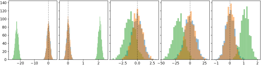
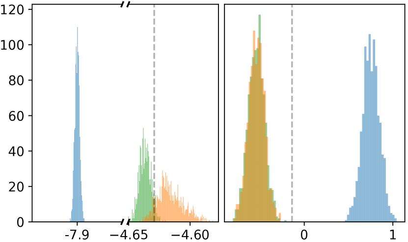
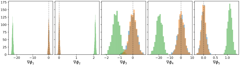
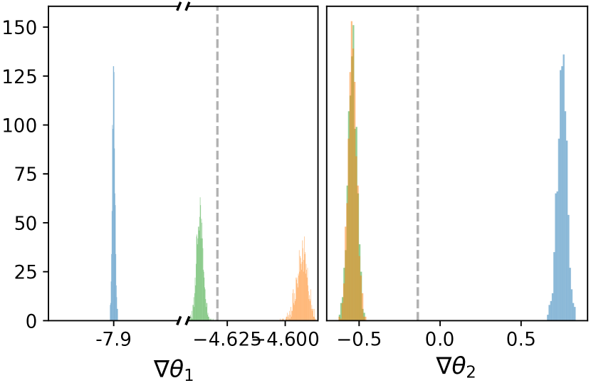
Figure 4: Gradient estimates of IWAE, AESMC, MCFO by Automatic Differentiation and analytic gradient of marginal log-likelihood w.r.t. generative and proposal parameters at the same optima as Figure 1; Top:K = 10000, Low: K = 100000.

Methods	K	$\triangledown\phi_{1}$	$\triangledown\phi_{2}$	$\triangledown\phi_{3}$	$\triangledown\phi_{4}$	$\triangledown\phi_{5}$
MCFO	1	0.45 $\pm$ 104.50	-0.05 $\pm$ 10.01	-0.97 $\pm$ 82.39	2.19 $\pm$ 870.35	0.07 $\pm$ 27.33
AESMC		-29.34 $\pm$ 108.92	2.33 $\pm$ 10.11	1.75 $\pm$ 90.75	-27.07 $\pm$ 904.10	1.35 $\pm$ 31.45
IWAE		1.24 $\pm$ 106.79	0.09 $\pm$ 3.29	-0.35 $\pm$ 89.99	-12.45 $\pm$ 995.37	0.89 $\pm$ 30.07
MCFO	10	0.29 $\pm$ 34.84	-0.03 $\pm$ 3.24	-0.57 $\pm$ 27.40	1.99 $\pm$ 284.15	-0.05 $\pm$ 9.33
AESMC		-22.81 $\pm$ 35.04	2.12 $\pm$ 3.25	-0.92 $\pm$ 27.70	-22.49 $\pm$ 294.92	0.88 $\pm$ 9.49
IWAE		-0.96 $\pm$ 35.46	0.09 $\pm$ 3.29	-0.35 $\pm$ 28.85	-9.80 $\pm$ 284.94	0.65 $\pm$ 10.00
MCFO	100	-0.37 $\pm$ 10.77	0.04 $\pm$ 1.00	-0.25$\pm$ 8.52	-3.21 $\pm$ 86.13	0.10 $\pm$ 2.87
AESMC		-22.13 $\pm$ 10.59	2.05 $\pm$ 0.98	-1.38 $\pm$ 8.99	-19.99 $\pm$ 91.75	1.10$\pm$ 3.04
IWAE		0.22 $\pm$ 11.11	-0.02 $\pm$ 1.03	-0.27 $\pm$ 9.61	-3.93 $\pm$ 98.78	0.08 $\pm$ 3.35
MCFO	1000	0.11 $\pm$ 3.39	0.00 $\pm$ 0.31	-0.04 $\pm$ 2.75	-0.19 $\pm$ 27.93	0.02 $\pm$ 0.93
AESMC		-22.39 $\pm$ 3.42	2.08 $\pm$ 0.32	-1.38 $\pm$ 2.87	-20.17$\pm$ 29.54	1.12 $\pm$ 0.99
IWAE		0.13 $\pm$ 3.58	-0.01 $\pm$ 0.33	-0.01 $\pm$ 2.89	-0.13$\pm$ 30.07	0.01 $\pm$ 1.01
MCFO	10000	-0.04 $\pm$ 1.10	0.00 $\pm$ 0.10	-0.02 $\pm$ 0.85	-0.31 $\pm$ 8.76	0.01 $\pm$ 0.29
AESMC		-22.55 $\pm$ 1.12	2.09 $\pm$ 0.10	-1.27 $\pm$ 0.91	-19.48 $\pm$ 9.18	1.10$\pm$ 0.31
IWAE		-0.01 $\pm$ 1.15	0.00 $\pm$ 0.11	-0.03 $\pm$ 0.91	-0.09 $\pm$ 9.49	0.01 $\pm$ 0.32
MCFO	100000	-0.01 $\pm$ 0.33	0.00 $\pm$ 0.031	0.01 $\pm$ 0.28	0.09 $\pm$ 2.79	0.00 $\pm$ 0.092
AESMC		-22.56$\pm$ 0.34	2.09 $\pm$ 0.032	-1.27 $\pm$ 0.27	-19.57 $\pm$ 2.73	1.11 $\pm$ 0.092
IWAE		0.00 $\pm$ 0.34	0.00 $\pm$ 0.032	0.00 $\pm$ 0.29	-0.04 $\pm$ 2.97	0.00 $\pm$ 0.099

Methods	K	$\triangledown\theta_{1}$	$\triangledown\theta_{2}$
MCFO	10	-4.64 $\pm$ 0.14	-0.52 $\pm$ 2.94
AESMC		-4.63 $\pm$ 0.14	-0.45 $\pm$ 2.81
IWAE		-7.93 $\pm$ 0.059	0.51 $\pm$ 2.94
MCFO	100	-4.64$\pm$0.046	-0.51 $\pm$0.88
AESMC		-4.64 $\pm$ 0.046	-0.54 $\pm$ 0.92
IWAE		-7.93 $\pm$ 0.020	0.71 $\pm$ 0.99
MCFO	1000	-4.63 $\pm$0.018	-0.55$\pm$0.28
AESMC		-4.64 $\pm$ 0.015	-0.55 $\pm$ 0.29
IWAE		-7.93$\pm$0.0060	0.75 $\pm$0.30
MCFO	10000	-4.62$\pm$0.0056	-0.54 $\pm$0.089
AESMC		-4.64 $\pm$ 0.0046	-0.54$\pm$0.092
IWAE		-7.93$\pm$0.00189	0.75 $\pm$0.095
MCFO	100000	-4.59 $\pm$ 0.0024	-0.54 $\pm$ 0.026
AESMC		-4.64 $\pm$ 0.0015	-0.54$\pm$ 0.027
IWAE		-7.93$\pm$ 0.00059	0.75 $\pm$ 0.030

Table 4: The mean and standard deviation of gradient estimates with respect to parameters $\boldsymbol{\phi}$ and $\boldsymbol{\theta}$ reported in Figure 1 and 4.

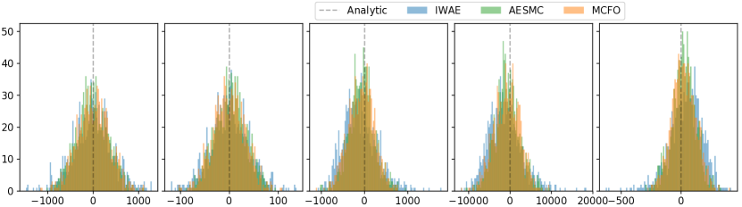
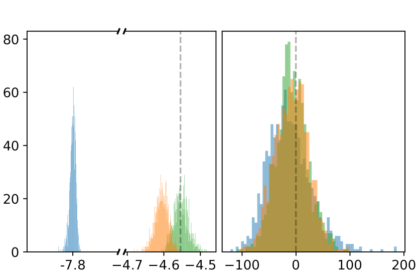
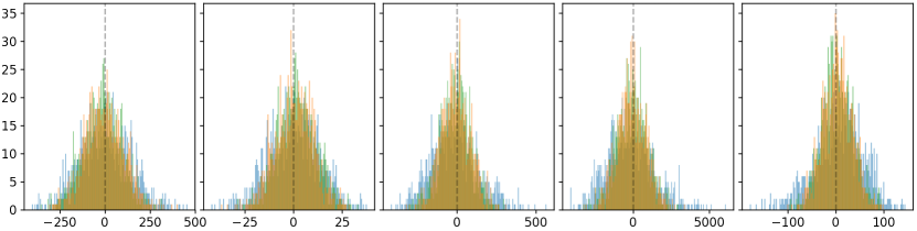
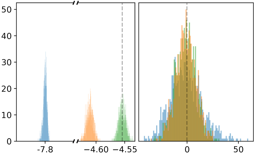
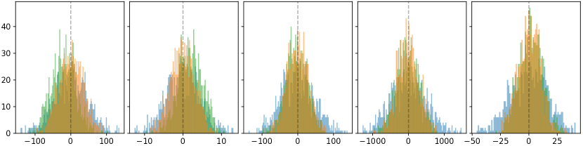
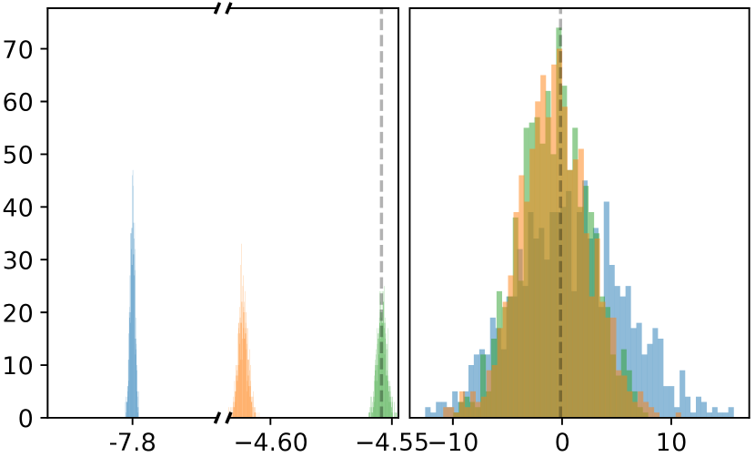
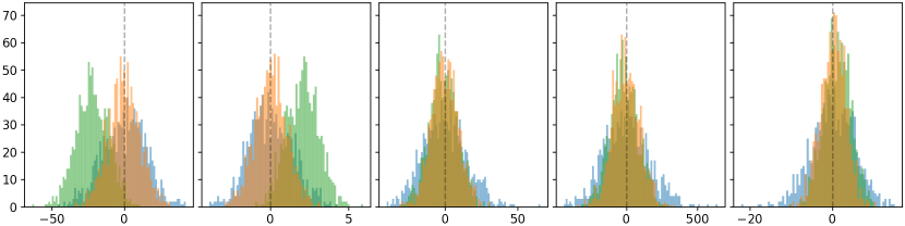
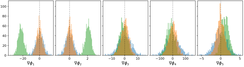
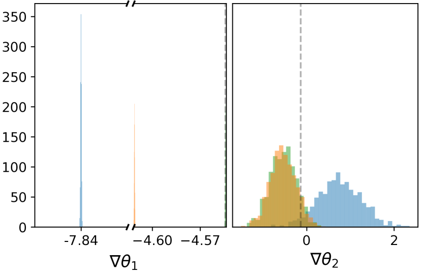
Figure 5: Gradient estimates of IWAE, AESMC, MCFO with respect to generative and proposal parameters at their optima with smaller variance of observation model, $\Sigma_{R}$, under different $K=10,100,1000,10000,100000$ from top to bottom respectively.

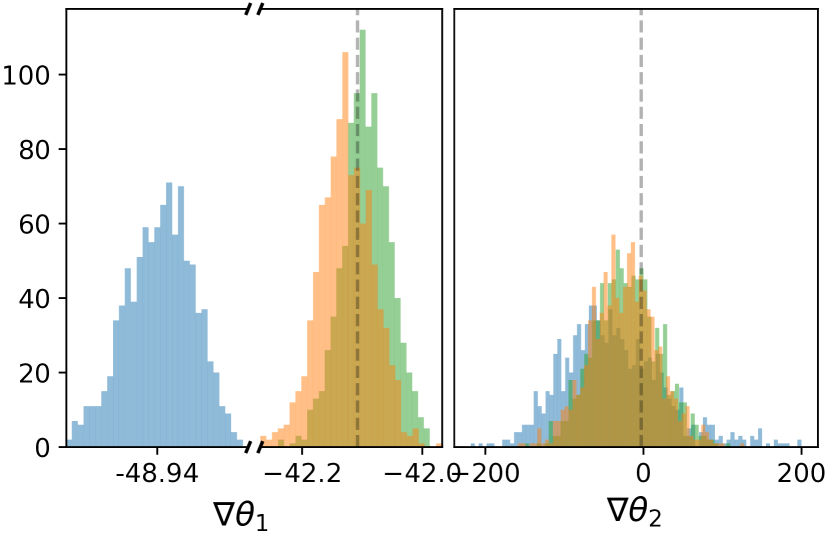
(a) K=10

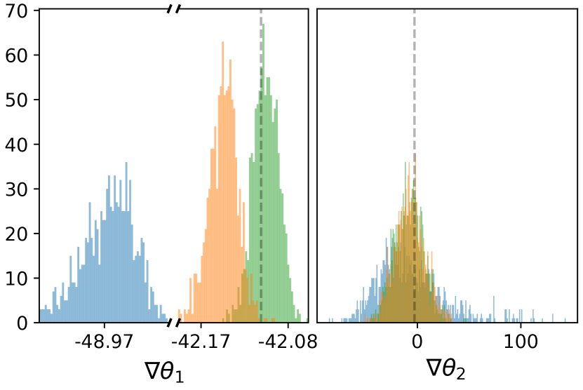
(b) K=100

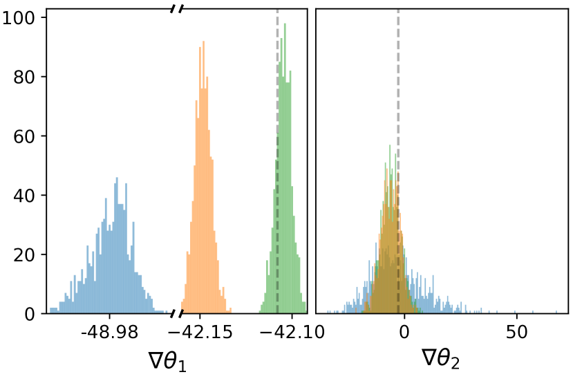
(c) K=1000

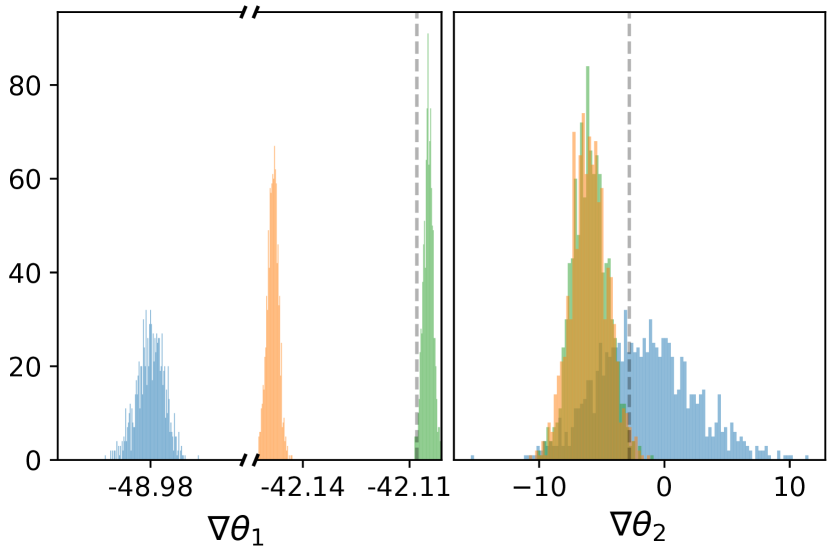
(d) K=10000

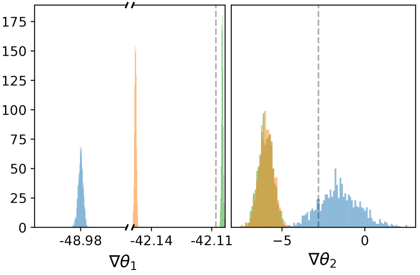
(e) K=100000

Figure 6: Gradient estimates of IWAE, AESMC, MCFO with respect to generative parameters, $\boldsymbol{\theta}$ at non-optima with different numbers of samples $K$ as 10, 100, 1000, 10000, 100000 respectively.

D Experiment on LGSSM

D.1 Gradient Estimate on LGSSM

Figure 4 shows gradient estimates with the numbers of samples $K=\{10000,100000\}$ at the same optima as Figure 1 when LGSSM parameters are set as: $\theta_{1}=0.9$, $\theta_{2}=10$, $\mu_{0}=0.5$, $\sigma_{0}=1.0$, $\Sigma_{Q}=1.0$, $\Sigma_{R}=1.0$. The bias in the estimates of $\triangledown\boldsymbol{\phi}$ by AESMC is distinguished and does not reduce with increasing $K$, while that by IWAE and MCFO is close to the true gradient. The variance of estimates on both $\boldsymbol{\theta}$ and $\boldsymbol{\phi}$ decreases at the order of $\mathcal{O}(1/K)$ (the standard deviation decreases at $\mathcal{O}(1/\sqrt{K})$ in Table 4) while the bias reduces substantially only when $K$ is small i.e. from 10 to 100.

It is found that the bias and variance reduction of gradient estimates are not uniform in the parameter space. For instance, Figure 5 shows the gradient estimates when observation variance $\Sigma_{R}$ is set as 0.01, which is lower than Figure 1 and Figure 4. The variance of gradient estimates in Figure 5 have higher variance on $\triangledown\boldsymbol{\phi}$ and $\triangledown\theta_{2}$ but lower on $\triangledown\theta_{1}$ for all three methods. Although the bias on $\triangledown\boldsymbol{\phi}$ is less distinguishable than in Figure 1, it cannot be removed with increasing the number of samples.

Except for the gradient estimates at the parameters’ optima, Figure 6 illustrates the estimates of gradient $\triangledown\boldsymbol{\theta}$ at non-optima, which of the generative parameters $\boldsymbol{\theta}$ are set to $\theta_{1}=0.6,\theta_{2}=8$. To compare to the analytic gradients, the local optima of proposal parameters are used for all surrogate objectives. The estimates by IWAE have higher variance and bias in $\theta_{1}$, but lower bias in $\theta_{2}$. Estimates by AESMC and MCFO have similar bias and variance on $\theta_{2}$ and $\theta_{1}$.

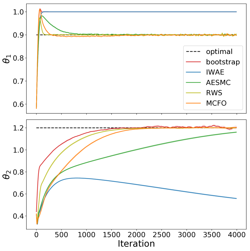
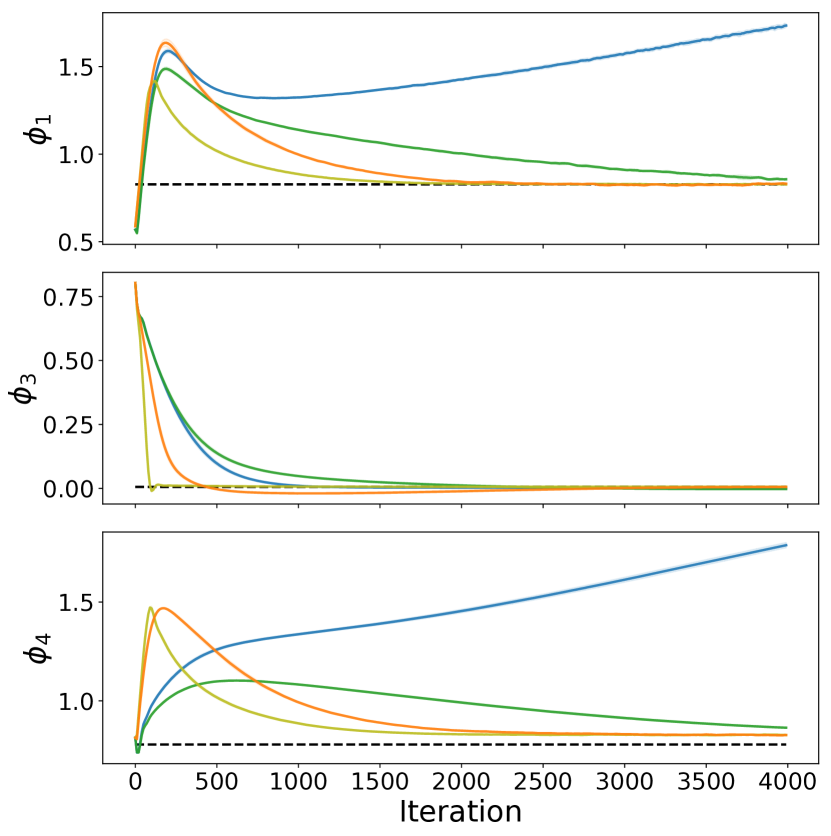
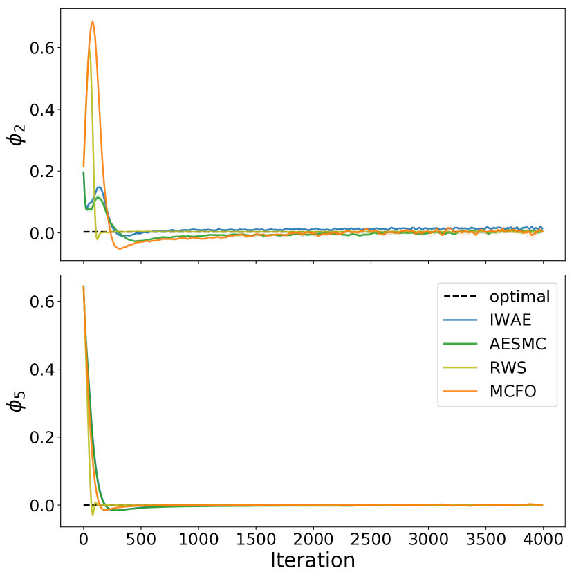
Figure 7: Parameters of generative and proposal, $\boldsymbol{\theta}$ and $\boldsymbol{\phi}$ during the training as Figure 2.

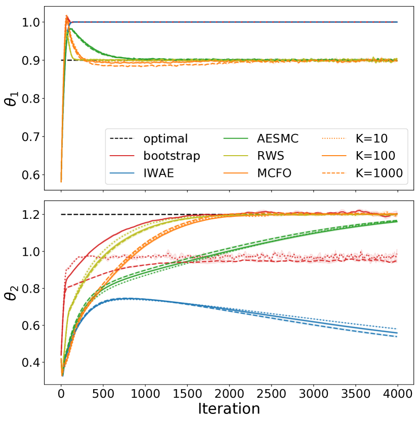
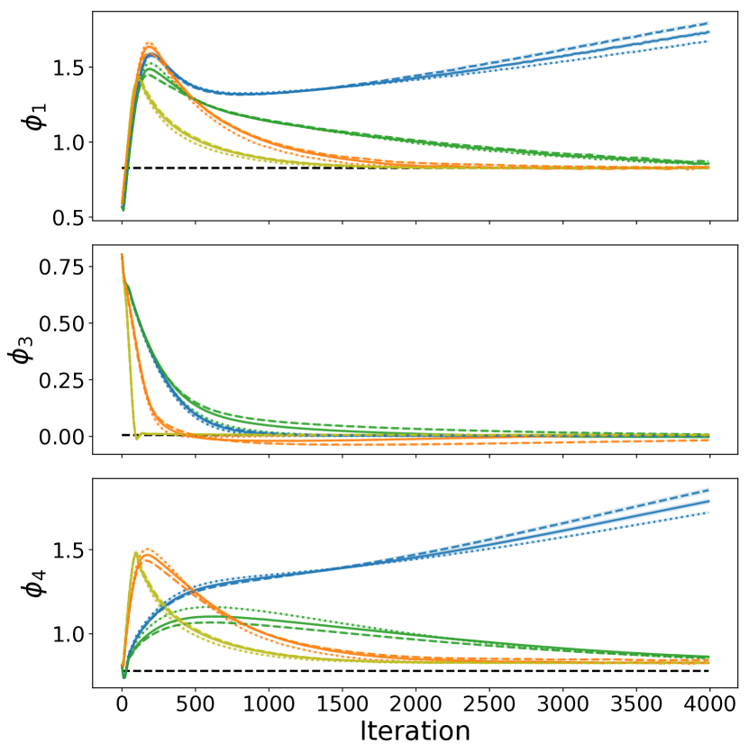
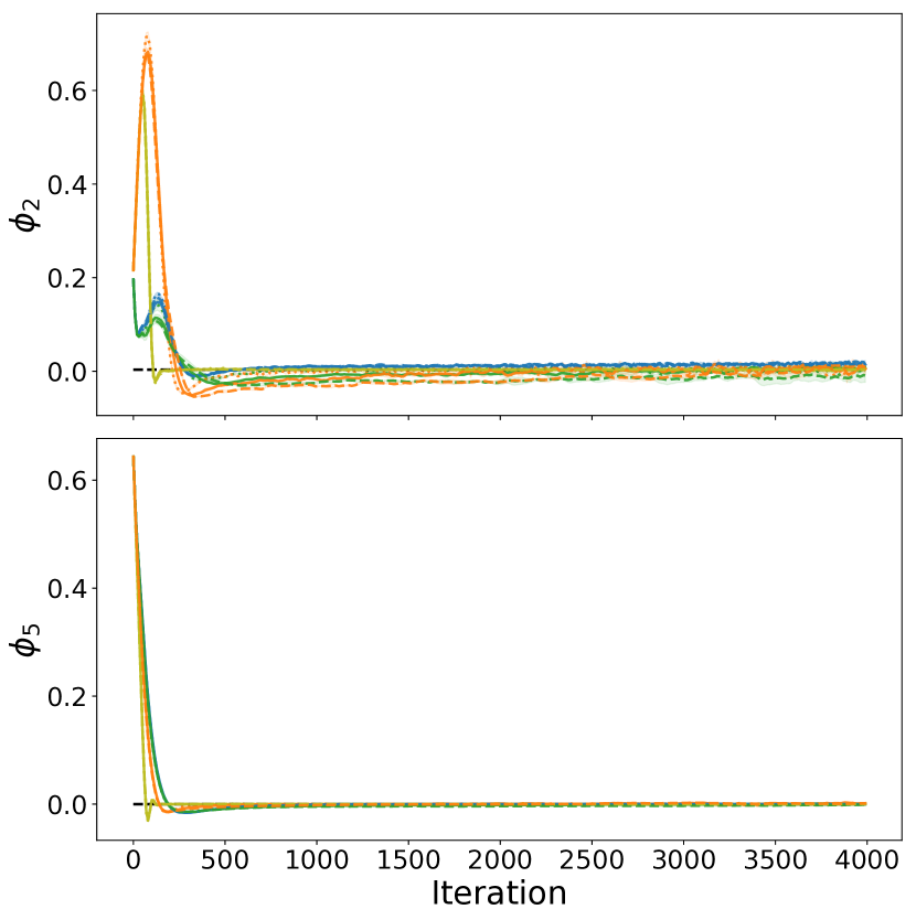
Figure 8: Learning of generative and proposal parameters for LGSSM with different numbers of samples. Top left: Negative marginal log-likelihoods on test data and gradient norms of all parameters. Top right: Generative model parameters $\theta_{1}$ and $\theta_{2}$. Bottom left: 3 proposal weights $\phi_{1}$, $\phi_{3}$ and $\phi_{4}$. Bottom right: 2 bias parameters $\phi_{2}$ and $\phi_{5}$. Lines indicate the average of 3 random seed trainings and shaded areas for standard deviation.

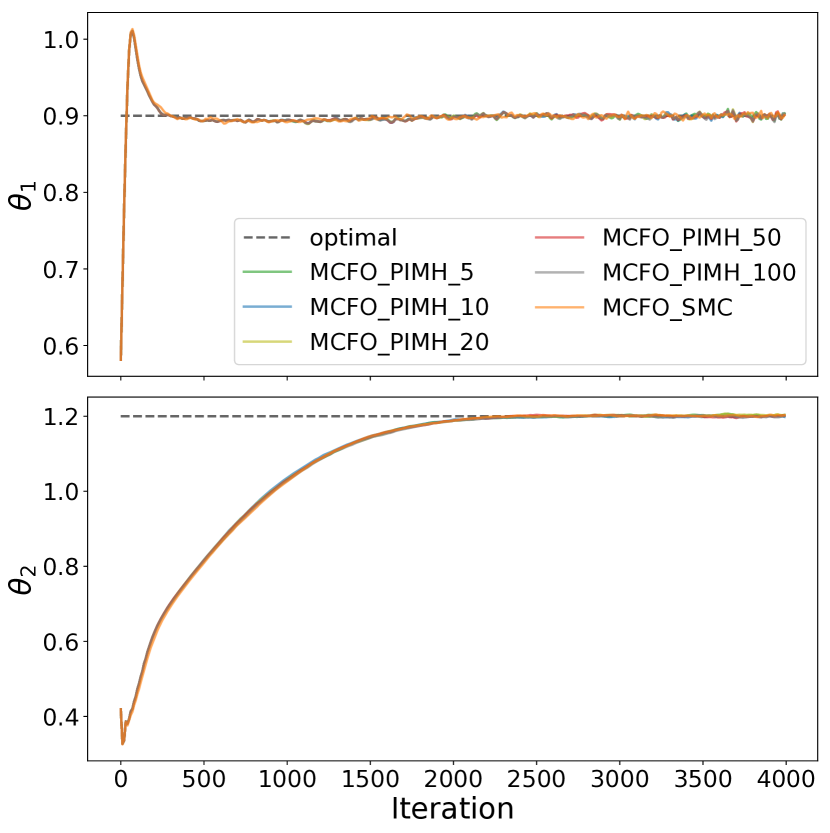
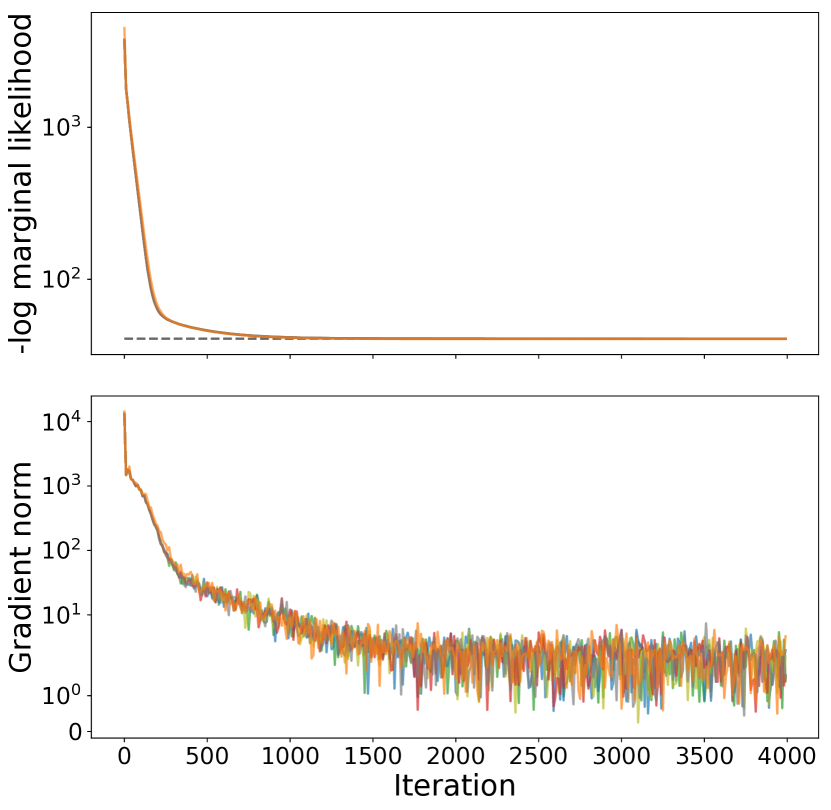
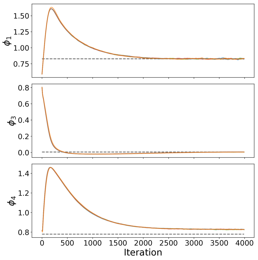
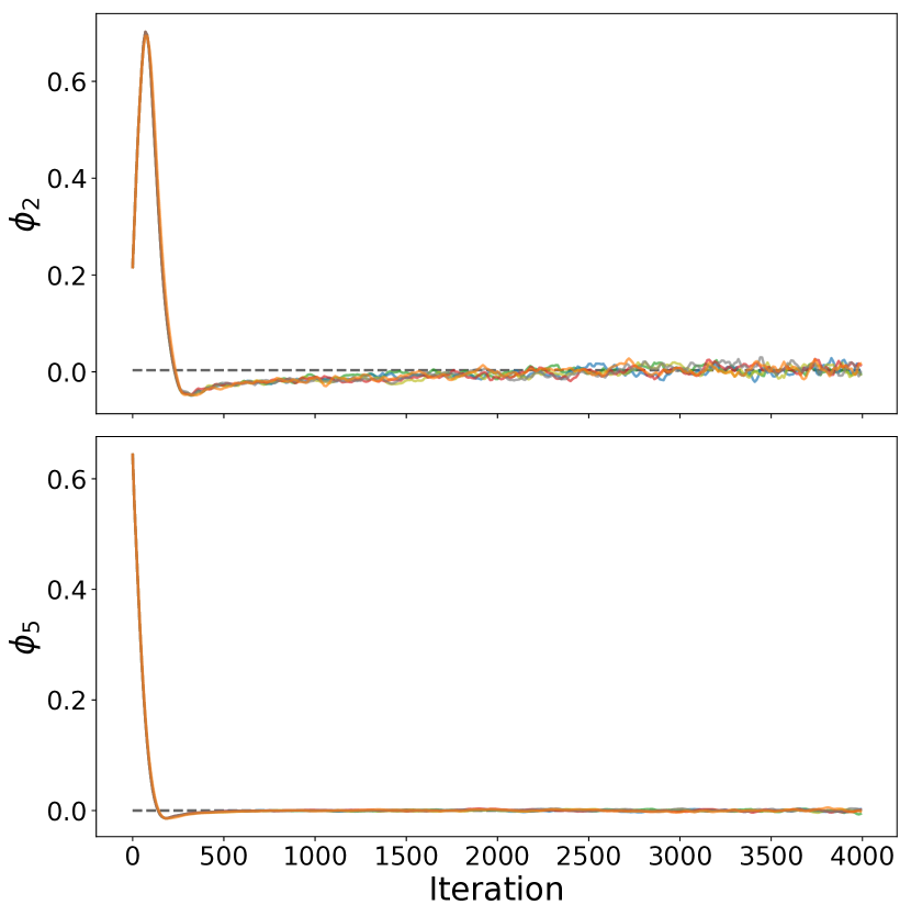
Figure 9: Top left: Generative model parameters $\theta_{1}$ and $\theta_{2}$. Top right: Negative marginal log-likelihoods on test data and gradient norms of all parameters. Bottom left: 3 proposal weights $\phi_{1}$, $\phi_{3}$ and $\phi_{4}$. Bottom right: 2 bias parameters $\phi_{2}$ and $\phi_{5}$. Lines indicate on different samplers and numbers of MH iterations.

D.2 Learning Generative and Proposal Parameters

The training and test datasets are generated by LGSSM with parameters $\mu_{0}=0.5$, $\sigma_{0}=1$, $\theta_{1}=0.9$, $\theta_{2}=1.2$, $\Sigma_{Q}=1.0$, $\Sigma_{R}=0.01$. We use Adam optimizer with default settings and the learning rate is constant as 0.01 for all methods. The numbers of samples for learning generative and proposal parameters are chosen from 10, 100, 1000.

Figure 7 shows the convergence of parameters, $\boldsymbol{\theta}$ and $\boldsymbol{\phi}$, during the same training as Figure 2. MCFO and RWS converge faster than other methods, while IWAE and bootstrap fail to converge to the optimum of parameters. In addition to $K=100$, Figure 8 shows the training when $K=10,1000$. The convergences of parameters are similar for AESMC, RWS and MCFO with different $K$ while bootstrap and IWAE are more sensitive to $K$. More samples accelerate convergence marginally on $\boldsymbol{\theta}$ while making $\boldsymbol{\phi}$ slower to converge. Figure 9 shows the comparisons of MCFO-SMC and MCFO-PIMH, using gradient estimates by SMC and PIMH with different numbers of MH iterations. For the simple LGSSM, MCFO-PIMH converges slightly faster that the early overshoot is restricted, compared to MCFO-SMC, but increasing numbers of MH iterations does not make much difference on this simple learning task.

E Pendulum Video Sequences

To evaluate MCFOs on more general state space models, we create a video sequence dataset of a single pendulum system as inspired by [Le et al., 2018]. Different to [Le et al., 2018], the SSM defined here has more complex latent trajectories than a random walk. The latent state space model of a single pendulum system is defined with angle $\omega$ and angular velocity $\dot{\omega}$ by:

$$\dot{\omega}_{t+1}=\frac{3}{ml^{2}}(mg\frac{l}{2}\sin\varphi_{t})\Delta t+\dot{\omega}_{t},$$

$$\omega_{t+1}=\dot{\omega}_{t}\Delta t+\omega_{t},$$

$$\begin{bmatrix}\dot{\omega}_{t+1}\\ \varphi_{t+1}\end{bmatrix}=g(\begin{bmatrix}\dot{\omega}_{t}\\ \omega_{t}\end{bmatrix})+\mathcal{N}(0,0.1^{2}),$$

where $\Delta t=0.05$, $g=10$, $m=1$, $l=1$ is specified in gym to create video sequences by projecting the angles of pendulum, $\omega$ to $32\times 32$ grayscale images as the Bernoulli distribution of binary observations.

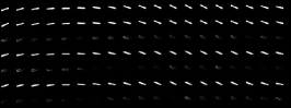
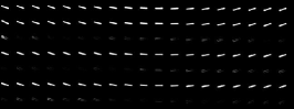
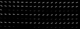
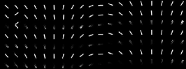
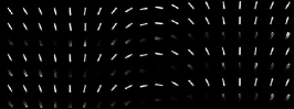
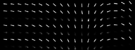
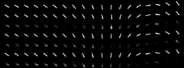
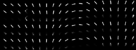
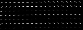
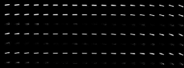
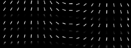
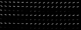
Figure 10: More sequence examples of filtering and one-step prediction by AESMC, MCFO-SMC and MCFO-PIMH with $K=100$. The first row is Bernoulli observations, followed by the one-step predictions and the absolute differences of predictions and observations of AESMC, MCFO-SMC and MCFO-PIMH.

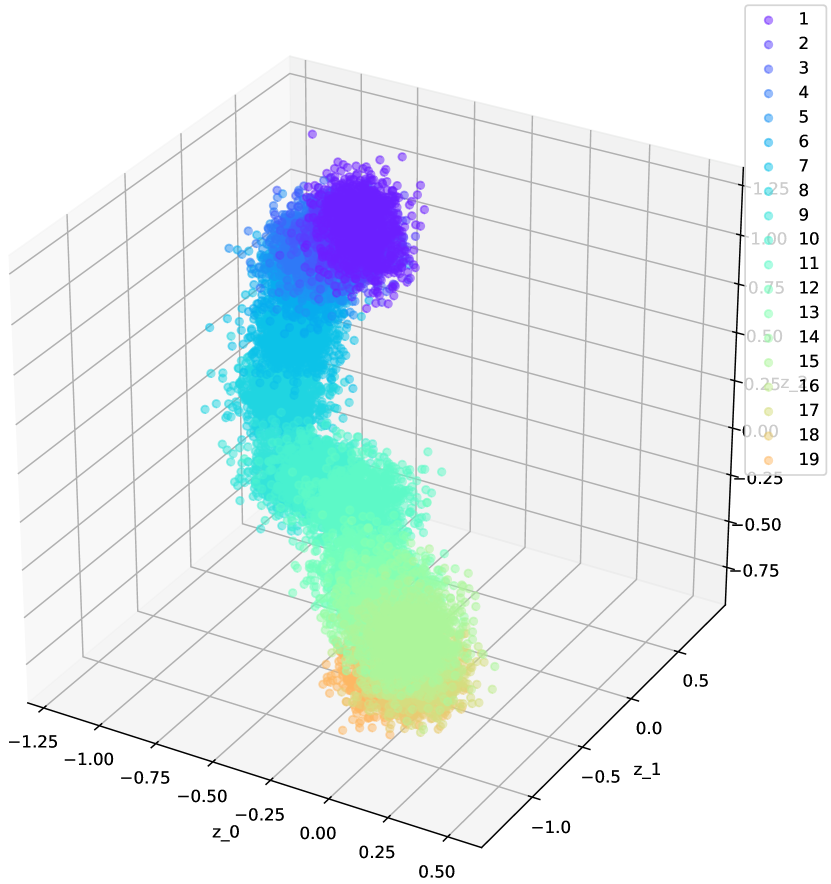
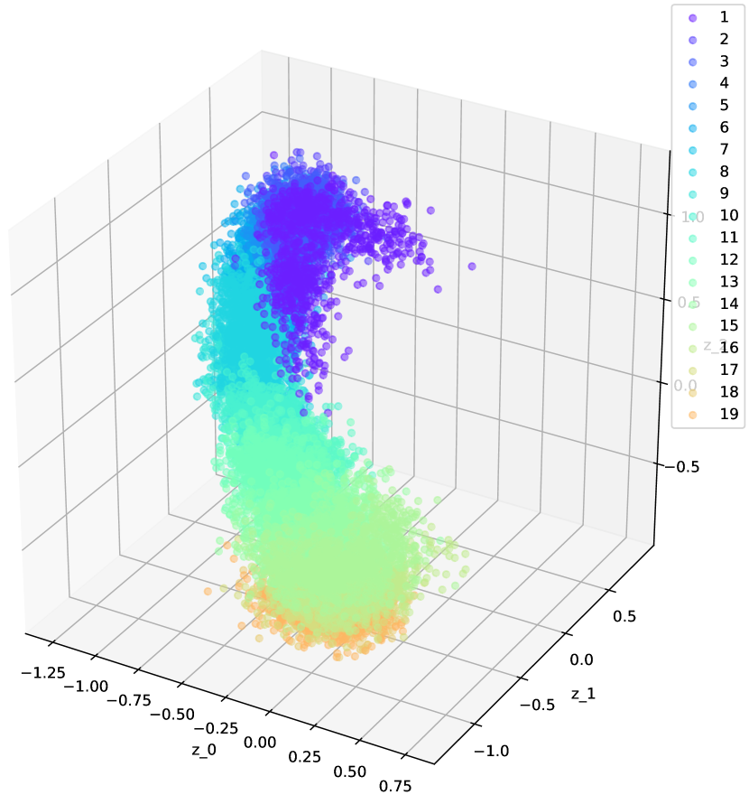
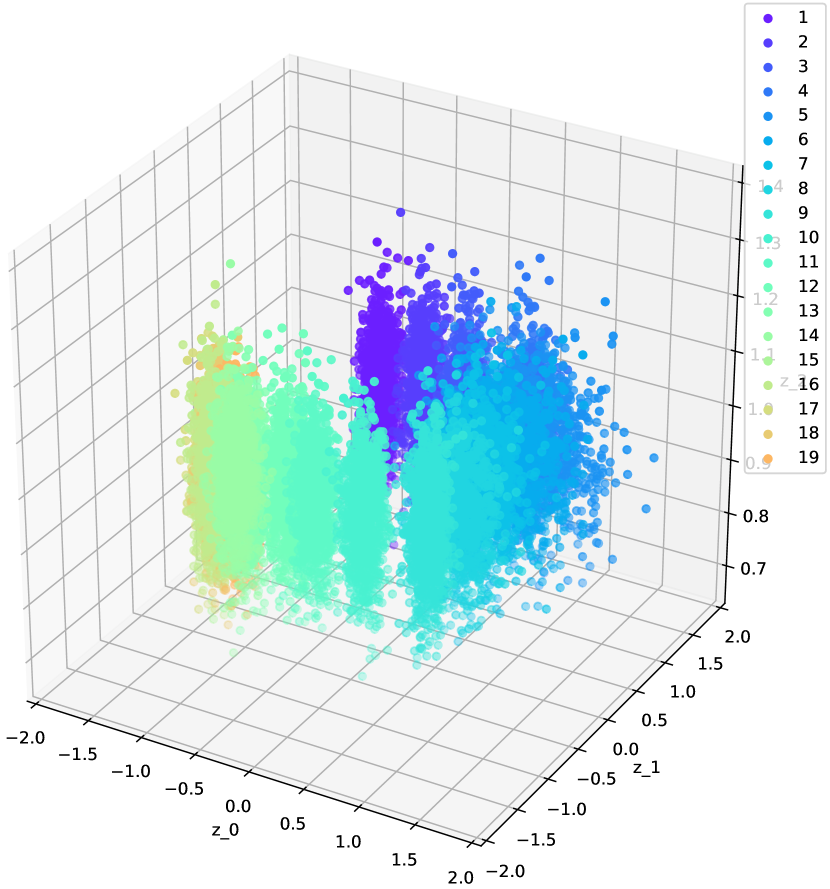
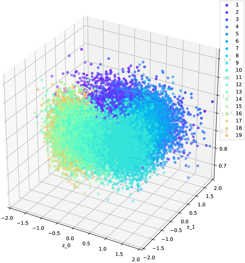
Figure 11: Visualization of 1000 samples of filtering and one-step ahead prediction in latent space; left is filtering inference samples and right is one-step ahead prediction samples. Top: AESMC-100. Bottom: MCFO-SMC-100.

All training by different objectives use the same generative and proposal model definitions. The latent dimension is set as 3 and all distributions on the latent variables are assumed to be Gaussian. The transition model $p_{\boldsymbol{\theta}}(\mathbf{z}_{t}|\mathbf{z}_{t-1})$ is specified as $\mathcal{N}(\mathbf{z}_{t};\boldsymbol{\mu}_{\boldsymbol{\theta}}(\mathbf{z}_{t-1}),\boldsymbol{\sigma}_{\boldsymbol{\theta}}^{2}(\mathbf{z}_{t-1}))$ with its mean and variance parameterized by Multi-layer perceptrons (MLPs) with 1 hidden layer of 64 units. The observation model $p_{\boldsymbol{\theta}}(\mathbf{x}_{t}|\mathbf{z}_{t})$ is assumed to be factorized Bernoulli distribution $\text{Bern}(\mathbf{x}_{t};\boldsymbol{\mu}_{\boldsymbol{\theta}}(\mathbf{z}_{t}))$, its mean is parameterized by a 4-hidden-layer MLP with 16, 64, 512, 2048 units. Instead of mixing $\mathbf{z}_{t-1}$ and $\mathbf{x}_{t}$ at first layer of NN, the proposal model $q_{\boldsymbol{\phi}}(\mathbf{z}_{t}|\mathbf{z}_{t-1},\mathbf{x}_{t})\sim\mathcal{N}(\mathbf{z}_{t};\boldsymbol{\mu}_{\boldsymbol{\phi}}(\mathbf{z}_{t-1},\mathbf{x}_{t}),\boldsymbol{\sigma}_{\boldsymbol{\phi}}^{2}(\mathbf{z}_{t-1},\mathbf{x}_{t}))$, first encodes $\mathbf{x}_{t}$ to low dimensional representation by a 2-hidden-layer MLP with 128, 32 units, then concatenates it with $\mathbf{z}_{t-1}$ to map to mean and variance by a 1-hidden-layer MLP with 32 units.

MCFO-SMC uses SMC while MCFO-PIMH uses PIMH with 5 MH iterations in gradient estimation. Adam optimizer with default parameter settings is used for all objectives. The initial learning rate is $1e-2$ and it decays every 10 iterations by a factor of 0.998 with the lowest rate as $1e-4$. For all MCFO-SMC and MCFO-PIMH, the number of samples to optimize proposal models is set to 10 while the numbers of samples for generative models are experimented by $\{10,20,50,100,200,500,1000\}$.

For evaluation of learned generative and proposal models, though the estimate negative log-likelihood is a common performance metric to report as in Section 4.2 and 4.4, it is not appropriate on this video sequences since it does not reflect how well the uncertainty is predicted on the observations comparing to the Bernoulli mean of observations. For instance, considering a binary pixel is sampled as 1 from a Bernoulli with mean as 0.6 and two models that predict mean as 0.7 and 0.9, the cross-entropy in the log-likelihood will favor the later model, however, first model predicts mean more correctly. To address this, we instead implement another widely used one-step-ahead prediction error, defined as the sum of L2 norms between the ground truth and one-step ahead predictions, $\sum_{t=2}^{T}\|\tilde{\mathbf{x}}_{t}^{pred}-\mathbf{x}_{t}^{GT}\|_{2}$. The prediction in observation space, $\tilde{\mathbf{x}}_{t}^{pred}$, is defined by the Bernoulli mean of the predicted mean in latent space, $\tilde{\mathbf{z}}^{pred}_{t}\approx\mathbb{E}_{p(\mathbf{z}_{t}|\mathbf{z}_{t-1})p(\mathbf{z}_{t-1}|\mathbf{x}_{1:t-1})}[\mathbf{z}_{t}]$, which is estimated by the transition model and the inference by SMC.

Figure 10 shows more examples of filtering reconstructions and one-step ahead predictions by MCFO-SMC, MCFO-PIMH and AESMC as Figure 3. Qualitatively, MCFO-PIMH and MCFO-SMC have relatively lower prediction deviation from ground truth, compared to AESMC. BBesides predictions in observation space, we investigate the latent samples from the learned posterior and predict one-step ahead by learned transition model. Figure 11 shows that the manifold of latent variables by MCFO-SMC is more regulated than that of AESMC since MCFO implicitly regularize to learn more sample efficient proposal models and thus simpler generative models. For MCFO-SMC, the representation of the pendulum system angle is mainly encoded in the dimensions $z_{0}$ and $z_{1}$ while this disentanglement cannot be observed in AESMC. Table 5 shows the evaluations on the models learned by more number of samples $K$ as Table 2. When K increases to 200, 500, 1000, no statistically significant difference is observed, compared to 100.

Method	$K$	Prediction	ESS
AESMC	200	37.65 $\pm$ 0.23	80.64 $\pm$ 0.97
MCFO-SMC		34.24 $\pm$ 1.56	128.97 $\pm$ 2.06
MCFO-PIMH		33.80 $\pm$ 0.99	129.85 $\pm$ 1.75
AESMC	500	36.93 $\pm$ 0.27	78.51 $\pm$ 1.09
MCFO-SMC		34.21 $\pm$ 1.58	128.80 $\pm$ 2.10
MCFO-PIMH		33.74 $\pm$ 0.89	130.01 $\pm$ 2.11
AESMC	1000	36.73 $\pm$ 0.29	79.89 $\pm$ 1.89
MCFO-SMC		34.18 $\pm$ 1.72	126.99 $\pm$ 3.26
MCFO-PIMH		33.62 $\pm$ 1.06	125.08 $\pm$ 2.37

Table 5: One-step prediction errors and ESS on the test set of generative and proposal models learned by AESMC, MCFO-SMC, MCFO-PIMH with $K=200,500,1000$, evaluated by SMC with 1000 samples averaged over last 1000 iterations.

F Polyphonic Music Sequences

To evaluate MCFOs on non-Markovian data of high dimensions and complex temporal dependencies, we choose four polyphonic music datasets [Boulanger et al., 2012]. Each dataset contains a varied length of sequences, and we pre-process all notes to 88-dimensional binary vectors that space the whole range of piano from A0 to C8. To model temporal dependencies of polyphonic music sequences, the same VRNN [Chung et al., 2015] is implemented for MCFO-SMC, MCFO-PIMH, FIVO and IWAE reported in Table 3.

All distributions of latent and hidden states, $\mathbf{z}$ and $\mathbf{h}$, are assumed to be Gaussian, while the observation distributions are factorized Bernoulli distributions of 88 dimensions. Both dimensions of hidden and latent variables are set as 64. VRNN uses Long Short Term Memory (LSTM) to update the deterministic hidden state with internal memory states by $(\mathbf{h}_{t},\mathbf{c}_{t})=\mathbf{LSTM}(\mathbf{z}_{t},\mathbf{x}_{t},\mathbf{h}_{t-1},\mathbf{c}_{t-1})$. With the hidden states, the generation process of VRNN is factorized as $\prod_{t=1}^{T}p_{\boldsymbol{\theta}}(\mathbf{z}_{t}|\mathbf{h}_{t-1})p_{\boldsymbol{\theta}}(\mathbf{x}_{t}|\mathbf{z}_{t},\mathbf{h}_{t-1})$. The transition $p_{\boldsymbol{\theta}}(\mathbf{z}_{t}|\mathbf{h}_{t-1})$ and emission $p_{\boldsymbol{\theta}}(\mathbf{x}_{t}|\mathbf{z}_{t},\mathbf{h}_{t-1})$ are parameterized by MLPs with a hidden layer of the same size as the dimension of latent variables. A function, $\varphi(\cdot)$, is implemented by an MLP to better encode the observations and the proposal, $q_{\phi}(\mathbf{z}_{t}|\mathbf{h}_{t-1},\varphi(\mathbf{x}_{t}))$, models $\mathbf{h}_{t-1}$, the encoded history of observations $\mathbf{x}_{1:t-1}$, and encoded new observation $\varphi(\mathbf{x}_{t})$ by a MLP with a hidden layer of the same size as the number of latent variables.

All the trainings of VRNN by MCFO-SMC, MCFO-PIMH, FIVO, IWAE uses Adam optimizer with default parameter settings. The initial learning rate is set as $1e-4$ and decays to the lowest rate as $1e-6$.

References

• Andrieu et al. [2010] Christophe Andrieu, Arnaud Doucet, and Roman Holenstein. Particle markov chain monte carlo methods. Journal of the Royal Statistical Society: Series B (Statistical Methodology), 72(3):269–342, 2010.
• Baydin et al. [2017] Atılım Günes Baydin, Barak A Pearlmutter, Alexey Andreyevich Radul, and Jeffrey Mark Siskind. Automatic differentiation in machine learning: a survey. The Journal of Machine Learning Research, 18(1):5595–5637, 2017.
• Bayer and Osendorfer [2014] Justin Bayer and Christian Osendorfer. Learning stochastic recurrent networks. In NIPS 2014 Workshop on Advances in Variational Inference, 2014.
• Bornschein and Bengio [2015] Jörg Bornschein and Yoshua Bengio. Reweighted wake-sleep. In 3rd International Conference on Learning Representations, ICLR, 2015.
• Boulanger et al. [2012] Lewandowski Nicolas Boulanger, Yoshua Bengio, and Pascal Vincent. Modeling temporal dependencies in high-dimensional sequences: application to polyphonic music generation and transcription. In Proceedings of the 29th International Conference on International Conference on Machine Learning, pages 1881–1888, 2012.
• Brockman et al. [2016] Greg Brockman, Vicki Cheung, Ludwig Pettersson, Jonas Schneider, John Schulman, Jie Tang, and Wojciech Zaremba. Openai gym, 2016.
• Burda et al. [2016] Yuri Burda, Roger B. Grosse, and Ruslan Salakhutdinov. Importance weighted autoencoders. In 4th International Conference on Learning Representations, ICLR 2016, 2016.
• Chung et al. [2015] Junyoung Chung, Kyle Kastner, Laurent Dinh, Kratarth Goel, Aaron C Courville, and Yoshua Bengio. A recurrent latent variable model for sequential data. In Advances in neural information processing systems, pages 2980–2988, 2015.
• Domke and Sheldon [2018] Justin Domke and Daniel R Sheldon. Importance weighting and variational inference. In Advances in neural information processing systems, pages 4470–4479, 2018.
• Doucet and Johansen [2009] Arnaud Doucet and Adam M Johansen. A tutorial on particle filtering and smoothing: Fifteen years later. Handbook of nonlinear filtering, 12(656-704):3, 2009.
• Doucet et al. [2000] Arnaud Doucet, Simon Godsill, and Christophe Andrieu. On sequential monte carlo sampling methods for bayesian filtering. Statistics and computing, 10(3):197–208, 2000.
• Fraccaro et al. [2016] Marco Fraccaro, Søren Kaae Sønderby, Ulrich Paquet, and Ole Winther. Sequential neural models with stochastic layers. In Advances in neural information processing systems, pages 2199–2207, 2016.
• Fraccaro et al. [2017] Marco Fraccaro, Simon Kamronn, Ulrich Paquet, and Ole Winther. A disentangled recognition and nonlinear dynamics model for unsupervised learning. In Advances in Neural Information Processing Systems, pages 3601–3610, 2017.
• Goodfellow et al. [2014] Ian Goodfellow, Jean Pouget-Abadie, Mehdi Mirza, Bing Xu, David Warde-Farley, Sherjil Ozair, Aaron Courville, and Yoshua Bengio. Generative adversarial nets. In Advances in Neural Information Processing Systems, pages 2672–2680. 2014.
• Gu et al. [2015] Shixiang Shane Gu, Zoubin Ghahramani, and Richard E Turner. Neural adaptive sequential monte carlo. In Advances in neural information processing systems, pages 2629–2637, 2015.
• Jacob et al. [2017] Pierre E Jacob, John O’Leary, and Yves F Atchadé. Unbiased markov chain monte carlo with couplings. arXiv preprint arXiv:1708.03625, 2017.
• Kingma and Welling [2014] Diederik P. Kingma and Max Welling. Auto-encoding variational bayes. In 2nd International Conference on Learning Representations, ICLR 2014, 2014.
• Krishnan et al. [2017] Rahul G Krishnan, Uri Shalit, and David Sontag. Structured inference networks for nonlinear state space models. In Thirty-First AAAI Conference on Artificial Intelligence, 2017.
• Le et al. [2018] Tuan Anh Le, Maximilian Igl, Tom Rainforth, Tom Jin, and Frank Wood. Auto-encoding sequential monte carlo. In 6th International Conference on Learning Representations, ICLR, 2018.
• Maddison et al. [2017] Chris J Maddison, John Lawson, George Tucker, Nicolas Heess, Mohammad Norouzi, Andriy Mnih, Arnaud Doucet, and Yee Teh. Filtering variational objectives. In Advances in Neural Information Processing Systems, pages 6573–6583, 2017.
• Mnih and Gregor [2014] Andriy Mnih and Karol Gregor. Neural variational inference and learning in belief networks. In Proceedings of the 31th International Conference on Machine Learning, ICML, volume 32, pages 1791–1799, 2014.
• Mnih and Rezende [2016] Andriy Mnih and Danilo Rezende. Variational inference for monte carlo objectives. In International Conference on Machine Learning, pages 2188–2196, 2016.
• Mohamed et al. [2020] Shakir Mohamed, Mihaela Rosca, Michael Figurnov, and Andriy Mnih. Monte carlo gradient estimation in machine learning. J. Mach. Learn. Res., 21:132:1–132:62, 2020.
• Naesseth et al. [2018] Christian Naesseth, Scott Linderman, Rajesh Ranganath, and David Blei. Variational sequential monte carlo. In International Conference on Artificial Intelligence and Statistics, pages 968–977, 2018.
• Rainforth et al. [2018] Tom Rainforth, Adam R. Kosiorek, Tuan Anh Le, Chris J. Maddison, Maximilian Igl, Frank Wood, and Yee Whye Teh. Tighter variational bounds are not necessarily better. In Proceedings of the 35th International Conference on Machine Learning, ICML, pages 4274–4282, 2018.
• Rezende and Mohamed [2015] Danilo Rezende and Shakir Mohamed. Variational inference with normalizing flows. In International Conference on Machine Learning, pages 1530–1538, 2015.
• Roeder et al. [2017] Geoffrey Roeder, Yuhuai Wu, and David K Duvenaud. Sticking the landing: Simple, lower-variance gradient estimators for variational inference. In Advances in Neural Information Processing Systems, pages 6925–6934, 2017.
• Särkkä [2013] Simo Särkkä. Bayesian filtering and smoothing, volume 3. Cambridge University Press, 2013.