Simulating violation of causality using a topological phase transition

Abstract

We consider a topological Hamiltonian and establish a correspondence between its eigenstates and the resource for a causal order game introduced in Ref. brukner , known as process matrix. We show that quantum correlations generated in the quantum many-body energy eigenstates of the model can mimic the statistics that can be obtained by exploiting different quantum measurements on the process matrix of the game. This provides an interpretation of the expectation values of the observables computed for the quantum many-body states in terms of the success probabilities of the game. As a result, we show that the ground state (GS) of the model can be related to the optimal strategy of the causal order game. Subsequently, we observe that at the point of maximum violation of the classical bound in the causal order game, corresponding quantum many-body model undergoes a second-order quantum phase transition (QPT). The correspondence equally holds even when we generalize the game for a higher number of parties.

I Introduction

Game-theoretic realization of quantum properties related to any physical system often provides a better way of conceptualization of the underlying physical theory brukner ; game_theory0 ; game_theory1 ; game_theory2 ; game_theory3 ; game_theory4 ; game_theory5 ; game_theory_entanglement1 ; game_theory_entanglement2 ; game_theory_entanglement3 ; game_theory_nonlocality1 ; game_theory_nonlocality2 ; game_theory6 . For instance, violation of Bell inequality which is incompatible with the conjunction of locality and realism can be formulated in the game-theoretic realm using the Clauser–Horne–Shimony–Holt (CHSH) game CHSH . The key feature of any game theory consists of exploiting different strategies to optimize the cost function of the game. In this regard, there have been studies where it is shown that for certain game theory set-up, quantum strategies provide more advantages than their classical counterparts game_theory0 ; game_theory1 ; game_theory4 . This has led to further investigations for a deeper understanding of the role of entanglement acin_paper ; game_theory_entanglement1 ; game_theory_entanglement2 ; game_theory_entanglement3 and nonlocality game_theory_nonlocality1 ; game_theory_nonlocality2 in any quantum game theory scheme.

A particularly interesting application of quantum many-player games could be to find its connection with quantum many-body systems. To begin with, we can think that different energy eigenstates of any quantum many-body Hamiltonian can be considered as strategies adopted by the quantum particles to attain a configuration that satisfies the energy constraints. Hence, the total energy of the system resembles the cost function of any game theory scheme, and the GS of the model then corresponds to the optimal strategy adopted by the quantum particles to minimize the cost function of the game. This motivates us to introduce a formalism that relates quantum many-body Hamiltonians to an actual quantum game theory scheme in a more profound way. In particular, we consider a topological Hamiltonian and show that the energy eigenstates of the model can be related to the process matrix which is considered to be the main resource in the causal order game introduced in Ref. brukner by Oreshkov et al. We show that in this way, expectation values of certain non-commutative quantum observables computed for the quantum many-body eigenstates of the system can be interpreted as the success probabilities of the different strategies considered in the causal order game. Moreover, we find that such a correspondence results in a classification of the eigenstates of the model based on the potentiality of violation of the classical bound by the process matrices to which the eigenstates can be related. Interestingly, we find that the GS and the most excited state of the model thus can be related to non-causally ordered process matrices that provide optimal success probability in the causal order game. In addition to this, we identify that the maximum violation of classical bound in the causal order game corresponds to the point where in the thermodynamic limit, the quantum many-body model undergoes a second-order QPT.

We organize the article as follows. In Sec. II we introduce the quantum many-body Hamiltonian that we consider in our work. Thereafter, in Sec. III we summarize the key points of the causal order game. Sec. IV is devoted to introducing the formalism of our work and providing a correspondence between the quantum many-body system and quantum game theory scheme. In Sec. V, we provide a generalization of the results to a higher number of parties. We discuss choices of relevant order parameters for identification of QPT point in Sec. VI. We conclude and discuss future plans in Sec.VII.

II Model

We start our discussion by introducing the quantum many-body Hamiltonian in one-dimension that will be the main focus in our work. To have the initial set-up exactly similar to the conventional causal order game for two parties, the minimum system size we consider is $N=4$, for which the quantum many-body Hamiltonian reads as

$$\mathcal{H}(\theta)=-2\cos\theta\sum_{i=1}^{2}\sigma_{z}^{i}\sigma_{z}^{i+2}-\sin\theta\sum_{i=1}^{4}\sigma_{z}^{i}\sigma_{x}^{i+1}\sigma_{z}^{i+2},$$ (1)

where $\sigma_{i}^{k}$ are the Pauli matrices at site $k$ ($i\in x,y,z$) and we consider periodic boundary conditions (PBC). It is apparent that for this small system size the model can be diagonalized instantly. However, one can note that even for any arbitrary $N$, the model can be exactly diagonalized by first applying certain non-local unitary transformation on pair of sites and then mapping it to a free-fermionic model. We discuss the methodology in detail in Sec. V where we generalize the set-up for higher number of parties. The Hamiltonian is translationally invariant and comprises certain symmetries. In particular, it commutes with the terms $\sigma_{x}^{i}\sigma_{x}^{i+2}$. Now if we look at different parts of the Hamiltonian, then we can identify that $\sigma_{z}^{i}\sigma_{z}^{i+2}$ defines the Ising interaction between the non-nearest neighbor sites. Similarly, the second part, $\sigma_{z}^{i}\sigma_{x}^{i+1}\sigma_{z}^{i+2}$ defines the cluster Hamiltonian cluster_Ham1 between nearest-neighbor sites. These two quantum Hamiltonians are characteristically very different from each other. In particular, the GS of cluster Hamiltonian with PBC is non-trivial and it is also an example of symmetry-protected topological (SPT) state cluster_Ham2 . In the thermodynamic limit, the model exhibits a second-order QPT at $\theta_{c}=\frac{\pi}{4}$ which we discuss in details in Sec.VI.

The main aim of our article is to provide a formalism to relate the energy eigenstates of the above model to the resource of a suitable quantum game theory scheme. For that purpose, we propose that the causal order game introduced in brukner (see also causal_order_exp ; causal_order_more1 ; causal_order_more2 ; causal_order_more3 ; causal_order_more4 ) can indeed be a potential candidate to establish such correspondence. However, before going into the details of our formalism, we first briefly review the key points of the causal order game in the forthcoming section.

III Indefinite causal order revisited

In this section, we revisit a causal order game between two observers Alice and Bob situated far from each other in their respective laboratories which are completely isolated from the external world. Now at a given run of the game, each of them opens their laboratory once to receive a particle ($A_{1}$ for Alice and $B_{1}$ for Bob) on which they can perform certain operations and later once to send additional systems ($A_{2}$ and $B_{2}$, respectively) out of their laboratories. See schematic Fig. 1 for the arrangements of Alice’s and Bob’s quantum systems. Now consider the following task to be performed by them. Once they receive the systems in their respective laboratories, each of the parties tosses a coin to obtain random bits ‘$a$’ (for Alice) and ‘$b$’ (for Bob). The parties now have to guess each other’s random bit and they will do that following the value of an additional random bit ‘$b^{\prime}$’ that Bob has to generate: if $b^{\prime}=0$, Bob will have to communicate the bit $b$ to Alice, whereas if $b^{\prime}=1$, he will have to guess the bit $a$. Now let us denote Alice’s and Bob’s guess about each other’s random bit ($a$ and $b$) by $x$ and $y$, respectively. Hence, the game aims to maximize the success probability

$$P_{success}=\frac{1}{2}[P_{Alice}(x=b,b^{\prime}=0)+P_{Bob}(y=a,b^{\prime}=1)].$$ (2)

One can show that if all events obey causal order, no strategy can allow Alice and Bob to exceed the classical bound $P_{success}\leq P^{classical}_{success}=\frac{3}{4}$.

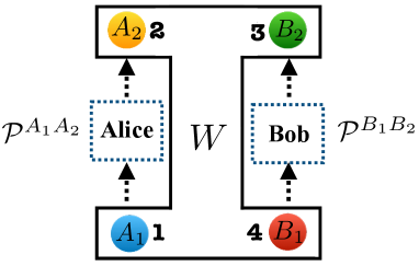
Figure 1: Schematic diagram of the arrangement of Alice’s ($A_{1},\leavevmode\nobreak\ A_{2}$) and Bob’s ($B_{1},\leavevmode\nobreak\ B_{2}$) quantum systems in the causal order game. The same arrangement was also indexed by 1, 2, 3, 4 to explore its correspondence with a quantum many-body Hamiltonian defined in Eq. (1).

In Ref. brukner it is shown that the bound can be violated if we consider the following scenario, where the systems share a process matrix (see Ref process_mat_def ) given by

$$W_{opt}(\theta)=\frac{1}{4}\Big{(}\mathbb{I}^{A_{1}A_{2}B_{1}B_{2}}+\cos\theta\sigma^{A_{2}}_{z}\sigma^{B_{1}}_{z}+\sin\theta\sigma^{A_{1}}_{z}\sigma^{B_{1}}_{x}\sigma^{B_{2}}_{z}\Big{)},$$

(3)

and apply certain measurement strategies. Note that the case considered in brukner corresponds to $\theta=\frac{\pi}{4}$, where the violation is maximal. Now the measurement strategies go as follows: Alice always measures her input qubit in the $z$-basis and obtains the bit $x$ which is her guess about Bob’s bit $b$. Thereafter, she encodes her random bit $a$ also in the $z$-basis. Therefore, the measurement operator in her part is given by

$$\mathcal{P}^{A_{1}A_{2}}_{b^{\prime}}=\frac{1}{2}\Big{(}\mathbb{I}^{{A_{1}}}+(-1)^{x}\sigma_{z}^{A_{1}}\Big{)}\frac{1}{2}\Big{(}\mathbb{I}^{{A_{2}}}+(-1)^{a}\sigma_{z}^{A_{2}}\Big{)}.$$ (4)

On the other hand, Bob’s measurement strategy has a dependence on the bit $b^{\prime}$. If $b^{\prime}=1$, he measures the input bit also in the $z$-basis obtaining $y$ which is his guess about Alice’s bit $a$. In this case, how he encodes his bit is no longer important and we can denote the operator by $\rho^{B_{2}}$, with ${\rm Tr}(\rho^{B_{2}})=1$. However, when $b^{\prime}=0$ he measures the input bit in the $x$-basis and encodes the output as follows: if $y=0$, $b=0\rightarrow|z_{+}^{B_{2}}\rangle$ and $b=1\rightarrow|z_{-}^{B_{2}}\rangle$. Otherwise, if $y=1$, $b=1\rightarrow|z_{+}^{B_{2}}\rangle$ and $b=0\rightarrow|z_{-}^{B_{2}}\rangle$. Hence, the measurement operator in Bob’s part reads as

$$\mathcal{P}^{B_{1}B_{2}}_{b^{\prime}} = b^{\prime}\frac{1}{2}\Big{(}\mathbb{I}^{{B_{1}}}+(-1)^{y}\sigma_{z}^{B_{1}}\Big{)}\rho^{B_{2}}$$

$$+ (1-b^{\prime})\frac{1}{2}\Big{(}\mathbb{I}^{{B_{1}}}+(-1)^{y}\sigma_{x}^{B_{1}}\Big{)}\frac{1}{2}\Big{(}\mathbb{I}^{{B_{2}}}+(-1)^{y+b}\sigma_{z}^{B_{2}}\Big{)}.$$

In this way, when $b^{\prime}=1$, a channel opens up between Alice’s output and Bob’s input and the success probability reads as

$$P_{Bob}(y=a,b^{\prime}=1) = \sum_{x}{\rm Tr}\Big{[}\frac{1}{2}\Big{(}\mathbb{I}^{{A_{1}}}+(-1)^{x}\sigma_{z}^{A_{1}}\Big{)}\frac{1}{2}\Big{(}\mathbb{I}^{{A_{2}}}+(-1)^{a}\sigma_{z}^{A_{2}}\Big{)}$$ (6)

$$\frac{1}{2}\Big{(}\mathbb{I}^{{B_{1}}}+(-1)^{y}\sigma_{z}^{B_{1}}\Big{)}\rho^{B_{2}}W_{opt}\Big{]},$$

$$= \frac{1+\cos\theta}{2}.$$

Similarly, when $b^{\prime}=0$, Bob opens a channel with memory between his output and Alice’s input which helps Alice to get the information of Bob’s random bit b with probability

$$P_{Alice}(x=b,b^{\prime}=0) = \sum_{y}{\rm Tr}\Big{[}\frac{1}{2}\Big{(}\mathbb{I}^{{A_{1}}}+(-1)^{x}\sigma_{z}^{A_{1}}\Big{)}\frac{1}{2}\Big{(}\mathbb{I}^{{A_{2}}}+(-1)^{a}\sigma_{z}^{A_{2}}\Big{)}$$ (7)

$$\frac{1}{2}\Big{(}\mathbb{I}^{{B_{1}}}+(-1)^{y}\sigma_{x}^{B_{1}}\Big{)}\frac{1}{2}\Big{(}\mathbb{I}^{{B_{2}}}+(-1)^{y+b}\sigma_{z}^{B_{2}}\Big{)}$$

$$W_{opt}\Big{]}=\frac{1+\sin\theta}{2}.$$

Hence, the total success probability is given by

$$P_{success}(\theta) = \frac{1}{2}\Big{[}P_{Alice}(x=b,b^{\prime}=0)+P_{Bob}(y=a,b^{\prime}=1)\Big{]},$$ (8)

$$= \frac{1}{4}\Big{[}2+\cos\theta+\sin\theta\Big{]}.$$

Therefore, the total success probability exceeds the classical bound $\frac{3}{4}$ for the region $0<\theta<\frac{\pi}{2}$ (see Fig. 2).

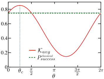
Figure 2: Plot of $\mathcal{K}_{avg}$ defined in Eq. (12) obtained for the GS $|\Psi(\theta)\rangle_{g}$ of $\mathcal{H}(\theta)$ as a function of $\theta$ (solid red) which coincides with the total success probability of the causal order game as defined in Eq. (8). The dashed green line corresponds to the maximal classical bound, $P_{success}^{classical}=\frac{3}{4}$. We can see that $\mathcal{K}_{avg}$ (equivalently $P_{success}$) exceeds $P_{success}^{classical}$ for $0<\theta<\frac{\pi}{2}$. At $\theta_{c}=\frac{\pi}{4}$, the point of maximal violation of causal bound, the observables $\Pi^{0}$ and $\Pi^{1}$ take same value $\frac{2+\sqrt{2}}{4}$.

IV Formalism

We devote this section to introduce the formalism necessary to establish the correspondence between the quantum Hamiltonian expressed in Eq. (1) and the causal order game introduced above. Towards this aim, we start with the GS of the model defined in Eq. (1) which has the following analytical form

$$|\Psi(\theta)\rangle_{g} = \cos^{2}\frac{\theta}{2}|\phi^{+}\rangle_{13}|\phi^{+}\rangle_{24}+\frac{\sin\theta}{2}\Big{(}|\phi^{+}\rangle_{12}|\psi^{+}\rangle_{34}$$ (9)

$$+ |\psi^{+}\rangle_{12}|\phi^{+}\rangle_{34}\Big{)}-\sin^{2}\frac{\theta}{2}|\psi^{+}\rangle_{13}|\psi^{+}\rangle_{24},$$

where $|\phi^{\pm}\rangle_{kl}=\frac{1}{\sqrt{2}}(|00\rangle_{kl}\pm|11\rangle_{kl})$ and $|\psi^{\pm}\rangle_{kl}=\frac{1}{\sqrt{2}}(|01\rangle_{kl}\pm|10\rangle_{kl})$ and the sites have been indexed according to the schematic presented in Fig. 1. Therefore, when $\theta\rightarrow 0$, we can identify the GS is the Ising ferromagnet between next-nearest neighbor sites $|\Psi(0)\rangle_{g}=|\phi^{+}\rangle_{13}|\phi^{+}\rangle_{24}$. Similarly, when $\theta\rightarrow\frac{\pi}{2}$, the GS becomes the cluster state $|\Psi(\frac{\pi}{2})\rangle_{g}=\frac{1}{4}\Pi_{i=1}^{4}\Big{(}\mathbb{I}+\sigma_{z}^{i}\sigma_{x}^{i+1}\sigma_{z}^{i+2}\Big{)}|0000\rangle=\frac{1}{2}\Big{(}|0+0+\rangle+|0-1-\rangle+|1-0-\rangle+|1+1+\rangle\Big{)}$, with $|\pm\rangle=\frac{1}{\sqrt{2}}(|0\rangle\pm|1\rangle)$. We now argue that the expectation value of a set of observables computed for $|\Psi(\theta)\rangle_{g}$ can be related to the success probabilities of strategies employed on the process matrix given in Eq. (3)

$${{}_{g}}\langle\Psi(\theta)|\Pi^{0}|\Psi(\theta)\rangle_{g}=\frac{1+\sin\theta}{2}\leftrightarrow P_{Alice}(x=b,b^{\prime}=0)=\frac{1+\sin\theta}{2},$$

$${{}_{g}}\langle\Psi(\theta)|\Pi^{1}|\Psi(\theta)\rangle_{g}=\frac{1+\cos\theta}{2}\leftrightarrow P_{Bob}(y=a,b^{\prime}=1)=\frac{1+\cos\theta}{2},$$ (10)

$$\text{where}\leavevmode\nobreak\ \leavevmode\nobreak\ \Pi^{0}=\frac{1}{2}\big{(}\mathbb{I}^{134}+\sigma_{z}^{1}\sigma_{z}^{3}\sigma_{x}^{4}\big{)},\Pi^{1} = \frac{1}{2}\big{(}\mathbb{I}^{24}+\sigma_{z}^{2}\sigma_{z}^{4}\big{)}.$$ (11)

This provides us with a scope to realize the success probability of different parties in the causal order game as the expectation values of two non-commutative operators $\Pi^{0}$ and $\Pi^{1}$ computed for the GS. Hence, the average of the correlators resemble the total success probability of the game (see Fig. 2),

$$\mathcal{K}_{avg} = \frac{{{}_{g}}\langle\Psi(\theta)|\Pi^{0}|\Psi(\theta)\rangle_{g}+{{}_{g}}\langle\Psi(\theta)|\Pi^{1}|\Psi(\theta)\rangle_{g}}{2}$$ (12)

$$= \frac{2+\cos\theta+\sin\theta}{4}.$$

Therefore, we argue that the GS $|\Psi(\theta)\rangle_{g}$ corresponds to a causally non-separable process matrix when $\mathcal{K}_{avg}$ exceeds a minimum value, $\frac{3}{4}$. Moreover, one can note that the point of maximum violation of the classical bound, $\theta_{c}=\frac{\pi}{4}$, corresponds to the QPT point of the model. This will be clear when we extend the model for a large system size. We discuss this in detail in Sec. VI.

A closer look at the three-body reduced density matrix derived from $|\Psi(\theta)\rangle_{g}$ reveals the reason for the operators $\Pi^{i}$’s to take the above values.

$$\rho^{134}_{g} = \frac{1}{8}\Big{[}\mathbb{I}^{134}+\cos\theta\sin\theta\sum_{i=1,3,4}\sigma_{x}^{i}+\cos\theta(\sigma_{z}^{1}\sigma_{z}^{3}-\sigma_{y}^{1}\sigma_{y}^{3})$$

$$+ \sigma_{x}^{1}\sigma_{x}^{3}+\cos\theta\sin\theta\sigma_{x}^{1}\sigma_{x}^{3}\sigma_{x}^{4}+\sin\theta(\sigma_{z}^{1}\sigma_{z}^{3}\sigma_{x}^{4}-\sigma_{y}^{1}\sigma_{y}^{3}\sigma_{x}^{4})\Big{]}.$$

From the above expression, we can easily see that the $zz$-correlation between sites 1 and 3 (equivalently between site 2 and 4) and the three-body correlation $zzx$ between sites 1 3 4 (equivalently correlation $zxz$ between sites (1 2 3), (2 1 4) and (2 3 4)) take the values $\cos\theta$ and $\sin\theta$, respectively, and makes $\rho^{134}_{g}$ structurally equivalent to $W_{opt}$, as expressed in Eq. (3). However, $\rho^{134}_{g}$ consist of more terms than $W_{opt}$. This naturally leads to the following question: What would be the correspondence for the other observables computed for the GS and other excited states of the model?

We now establish the relation between other excited states of the Hamiltonian $\mathcal{H}(\theta)$ together with the quantum observables computed for them to that of the strategies applied in the causal order game using the formalism we propose below.

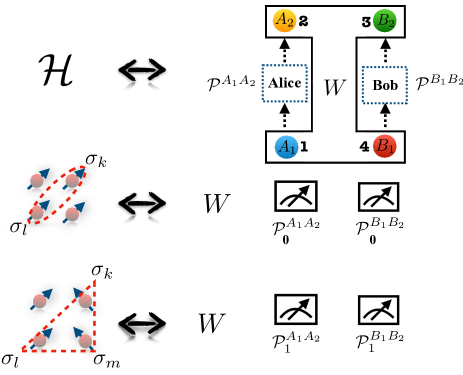
Figure 3: Schematic diagram of the analogy between quantum strategies exploited in causal order game that includes process matrix and quantum measurements and the strategies adopted by the quantum particles that consist of energy eigenstates and choice of certain physical observables.

i) Quantum many-body Hamiltonian and quantum game theory scheme: We first provide a realization of any quantum many-body Hamiltonian in terms of a quantum game theory scheme. In particular, we argue that the total energy of the system can be related to the pay-offs of any game theory. Therefore, the eigenstates of the model can be considered as different strategies adopted by the quantum particles to yield a particular value of energy. In this way, we can think that the GS corresponds to the optimal strategy applied by the quantum particles to minimize the total energy of the system or the pay-off function of the game. This lays out the initial set-up we need to provide a systematic comparison between a quantum many-body Hamiltonian and an actual game theory scheme. However, to relate the quantum many-body Hamiltonian $\mathcal{H}$ to the causal order game in a profound way, we need some additional aspects which we state in the next two axioms.

ii) Eigenstates of $\mathcal{H}(\theta)$ and process matrix of causal order game: In the case of the causal order game, as described above, all the participants agree on performing certain quantum measurements on the process matrix to optimize the success probability, which we call the strategies of the game. When those strategies are applied, quantum channels between different parts of the system may open up which essentially assists to communicate the information about the random bit to be guessed. In the quantum many-body systems, an analogy of this can be given by generalizing the notion of strategy introduced in the axiom i) as follows. When the quantum particles adopt a particular configuration satisfying the energy constraint, correlations may generate in different parts of the system. Hence, the notion of strategy in quantum many-body systems comprises of two constituents, the energy eigenstates and the choices of quantum operators quantifying different correlations in their subparts. A quantitative way of conceptualization of this correspondence is stated in the axiom below.

iii) Quantum observables and success probability: We propose that the expectation values of the relevant physical operators computed for the quantum many-body eigenstates of the model can be related to the success probability of different strategies of the causal order game.

We are now ready with the necessary tools to relate the GS and quantum observables computed for it with that of different strategies of the causal order game. We summarize the correspondence in Table 1 and a schematic representation of the same is presented in Fig. 3. For instance, in the first row of Table 1, we now establish correspondence between the expectation values of correlators $\sigma_{y}^{1}\sigma_{y}^{3}$, $\sigma_{y}^{1}\sigma_{y}^{3}\sigma_{x}^{4}$ and the probabilities obtained from the causal order game. For that purpose, similarly to Eq. (10), we compute the expectation values of two sets of observables $\Pi^{0}=\frac{1}{2}(\mathbb{I}^{134}+\sigma_{y}^{1}\sigma_{y}^{3}\sigma_{x}^{4})$ and $\Pi^{1}=\frac{1}{2}(\mathbb{I}^{13}+\sigma_{y}^{1}\sigma_{y}^{3})$ and compare it with the probabilities that can be obtained by applying the set of operators $\mathcal{P}^{A_{1}A_{2}}_{0(1)}$ and $\mathcal{P}^{B_{1}B_{2}}_{0(1)}$ defined in the table on a process matrix given by $W=\frac{1}{4}\Big{(}\mathbb{I}^{A_{1}A_{2}B_{1}B_{2}}-\cos\theta\sigma_{y}^{A_{2}}\sigma_{y}^{B_{1}}-\sin\theta\sigma_{y}^{A_{1}}\sigma_{x}^{B_{1}}\sigma_{y}^{B_{2}}\Big{)}$. One can realize that the outcomes coincide with that obtained in Eq. (10), for $W_{opt}(\theta+\pi)$.

No.	Strategy	Outcome
1	$\begin{array}[]{lcl}\begin{cases}|\Psi\rangle_{g},\\ \Pi^{0}=\frac{1}{2}(\mathbb{I}^{134}+\sigma_{y}^{1}\sigma_{y}^{3}\sigma_{x}^{4}),\Pi^{1}=\frac{1}{2}(\mathbb{I}^{13}+\sigma_{y}^{1}\sigma_{y}^{3}),\end{cases}\\ \hskip 20.48601pt\updownarrow\\ \begin{cases}W=\frac{1}{4}\Big{(}\mathbb{I}^{A_{1}A_{2}B_{1}B_{2}}-\cos\theta\sigma^{A_{2}}_{y}\sigma^{B_{1}}_{y}-\sin\theta\sigma^{A_{1}}_{y}\sigma^{B_{1}}_{x}\sigma^{B_{2}}_{y}\Big{)},\\ \mathcal{P}^{A_{1}A_{2}}_{0}=\frac{1}{2}\Big{(}\mathbb{I}^{A_{1}}+(-1)^{x}\sigma_{y}^{A_{1}}\Big{)}\frac{1}{2}\Big{(}\mathbb{I}^{A_{2}}+(-1)^{a}\sigma_{y}^{A_{2}}\Big{)},\\ \mathcal{P}^{B_{1}B_{2}}_{0}=\frac{1}{2}\Big{(}\mathbb{I}^{B_{1}}+(-1)^{y}\sigma_{x}^{B_{1}}\Big{)}\frac{1}{2}\Big{(}\mathbb{I}^{B_{2}}+(-1)^{y+b}\sigma_{y}^{B_{2}}\Big{)},\\ \mathcal{P}^{A_{1}A_{2}}_{1}=\frac{1}{2}\Big{(}\mathbb{I}^{A_{1}}+(-1)^{x}\sigma_{y}^{A_{1}}\Big{)}\frac{1}{2}\Big{(}\mathbb{I}^{A_{2}}+(-1)^{a}\sigma_{y}^{A_{2}}\Big{)},\\ \mathcal{P}^{B_{1}B_{2}}_{1}=\frac{1}{2}\Big{(}\mathbb{I}^{B_{1}}+(-1)^{y}\sigma_{y}^{B_{1}}\Big{)}\rho^{B_{2}}.\\ \end{cases}\end{array}$	$\begin{array}[]{lcl}{{}_{g}}\langle\Psi|\Pi^{0}\Psi\rangle_{g}&=&\frac{1-\sin(\theta)}{2}\\ &\updownarrow&\\ P_{Alice}(x=b,b^{\prime}=0)&=&\sum_{y}\Big{[}\text{Tr}\Big{(}\mathcal{P}_{0}^{A_{1}A_{2}}\mathcal{P}_{0}^{B_{1}B_{2}}W\Big{)}\Big{]}_{x=b}=\frac{1-\sin\theta}{2},\\ \\ {{}_{g}}\langle\Psi|\Pi^{1}|\Psi\rangle_{g}&=&\frac{1-\cos\theta}{2}\\ &\updownarrow&\\ P_{Bob}(y=a,b^{\prime}=1)&=&\sum_{x}\Big{[}\text{Tr}\Big{(}\mathcal{P}_{1}^{A_{1}A_{2}}\mathcal{P}_{1}^{B_{1}B_{2}}W\Big{)}\Big{]}_{y=a}=\frac{1-\cos\theta}{2}\end{array}$
2	$\begin{array}[]{lcl}\begin{cases}|\Psi\rangle_{g},\\ \Pi^{0}=\frac{1}{2}\mathbb{I}^{1234},\Pi^{1}=\frac{1}{2}(\mathbb{I}^{13}+\sigma_{x}^{1}\sigma_{x}^{3}),\end{cases}\\ \hskip 20.48601pt\updownarrow\\ \begin{cases}W=\frac{1}{4}\Big{(}\mathbb{I}^{A_{2}B_{1}}+\sigma_{x}^{A_{2}}\sigma_{x}^{B_{1}}\Big{)},\\ \mathcal{P}^{A_{1}A_{2}}_{1}=\frac{1}{2}\Big{(}\mathbb{I}^{A_{1}}+(-1)^{x}\sigma_{z}^{A_{1}}\Big{)}\frac{1}{2}\Big{(}\mathbb{I}^{A_{2}}+(-1)^{a}\sigma_{x}^{A_{2}}\Big{)},\\ \mathcal{P}^{B_{1}B_{2}}_{1}=\frac{1}{2}\Big{(}\mathbb{I}^{B_{1}}+(-1)^{y}\sigma_{x}^{B_{1}}\Big{)}\rho_{B_{2}}.\end{cases}\end{array}$	$\begin{array}[]{lcl}{{}_{g}}\langle\Psi|\Pi^{0}|\Psi\rangle_{g}&=&\frac{1}{2}\\ &\updownarrow&\\ P_{Alice}(x=b,b^{\prime}=0)&=&\frac{1}{2},\\ \\ {{}_{g}}\langle\Psi|\Pi^{1}|\Psi\rangle_{g}&=&1\\ &\updownarrow&\\ P_{Bob}(y=a,b^{\prime}=1)&=&\sum_{x}\Big{[}\text{Tr}\Big{(}\mathcal{P}_{1}^{A_{1}A_{2}}\mathcal{P}_{1}^{B_{1}B_{2}}W\Big{)}\Big{]}_{y=a}=1\end{array}$
3	$\begin{array}[]{lcl}\begin{cases}|\Psi\rangle_{g},\\ \Pi^{0}=\frac{1}{2}(\mathbb{I}^{134}+\sigma_{x}^{1}\sigma_{x}^{3}\sigma_{x}^{4}),\Pi^{1}=\frac{1}{2}(\mathbb{I}^{1234}),\end{cases}\\ \hskip 20.48601pt\updownarrow\\ \begin{cases}W=\frac{1}{4}\Big{(}\mathbb{I}^{A_{1}A_{2}B_{1}B_{2}}+\sin\theta\cos\theta\sigma^{A_{1}}_{x}\sigma^{B_{1}}_{x}\sigma^{B_{2}}_{x}\Big{)},\\ \mathcal{P}^{A_{1}A_{2}}_{0}=\frac{1}{2}\Big{(}\mathbb{I}^{A_{1}}+(-1)^{x}\sigma_{x}^{A_{1}}\Big{)}\frac{1}{2}\Big{(}\mathbb{I}^{A_{2}}+(-1)^{a}\sigma_{x}^{A_{2}}\Big{)},\\ \mathcal{P}^{B_{1}B_{2}}_{0}=\frac{1}{2}\Big{(}\mathbb{I}^{B_{1}}+(-1)^{y}\sigma_{x}^{B_{1}}\Big{)}\frac{1}{2}\Big{(}\mathbb{I}^{B_{2}}+(-1)^{y+b}\sigma_{x}^{B_{2}}\Big{)}.\end{cases}\end{array}$	$\begin{array}[]{lcl}{{}_{g}}\langle\Psi|\Pi^{0}|\Psi\rangle_{g}&=&\frac{1+\sin\theta\cos\theta}{2}\\ &\updownarrow&\\ P_{Alice}(x=b,b^{\prime}=0)&=&\sum_{y}\Big{[}\text{Tr}\Big{(}\mathcal{P}_{0}^{A_{1}A_{2}}\mathcal{P}_{0}^{B_{1}B_{2}}W\Big{)}\Big{]}_{x=b}=\frac{1+\sin\theta\cos\theta}{2},\\ \\ {{}_{g}}\langle\Psi|\Pi^{1}|\Psi\rangle_{g}&=&\frac{1}{2}\\ &\updownarrow&\\ P_{Bob}(y=a,b^{\prime}=1)&=&\frac{1}{2}\end{array}$

Table 1: Correspondence between strategies applied in causal order game to that of the strategies employed in quantum-many body systems. Here, we consider the GS of the model.

For the remaining correlators $\sigma_{x}^{1}\sigma_{x}^{3}$ and $\sigma_{x}^{1}\sigma_{x}^{3}\sigma_{x}^{4}$, we need to modify the causal order game to some extent. For example, for $\sigma_{x}^{1}\sigma_{x}^{3}$, when $b^{\prime}=1$ Alice assists Bob to guess her qubit like as the previous cases and the strategy now involves the operators $\mathcal{P}^{A_{1}A_{2}}_{1}$ and $\mathcal{P}^{B_{1}B_{2}}_{1}$ defined in the table, and the process matrix given by $W=\frac{1}{4}\Big{(}\mathbb{I}^{A_{2}B_{1}}+\sigma_{x}^{A_{2}}\sigma_{x}^{B_{1}}\Big{)}$. This results in $P_{Bob}(y=a,b^{\prime}=1)=1$, which coincides with the expectation value of the operator $\Pi^{1}=\frac{1}{2}(\mathbb{I}^{13}+\sigma_{x}^{1}\sigma_{x}^{3})$. However, when $b^{\prime}=0$, Bob becomes biased and does not want to communicate his random bit $b$ to Alice. Hence, Alice can guess Bob’s random bit with a probability $P_{Alice}(x=b,b^{\prime}=0)=\frac{1}{2}$, which coincides with the expectation value of the opertaor $\Pi^{0}=\frac{1}{2}\mathbb{I}^{1234}$. Therefore, in this case, the game consists of effectively only one quantum strategy ($b^{\prime}=1$) and the total success probability thus turns out to be $P_{success}=\frac{1}{2}\Big{[}P_{Alice}(x=b,b^{\prime}=0)+P_{Bob}(y=a,b^{\prime}=1)\Big{]}=\frac{3}{4}$. Similarly, for the three-body correlator $\sigma_{x}^{1}\sigma_{x}^{3}\sigma_{x}^{4}$ we consider the opposite scenario, i.e., in this case, Bob always assists Alice to guess his random qubit $b$ ($b^{\prime}=0$) and the strategy consists of measurement operators $\mathcal{P}^{A_{1}A_{2}}_{0}$ and $\mathcal{P}^{B_{1}B_{2}}_{0}$ defined in the table and the process matrix given by $W=\frac{1}{4}\Big{(}\mathbb{I}^{A_{1}A_{2}B_{1}B_{2}}+\sin\theta\cos\theta\sigma^{A_{1}}_{x}\sigma^{B_{1}}_{x}\sigma^{B_{2}}_{x}\Big{)}$, which yields $P_{Alice}(x=a,b^{\prime}=0)=\frac{1+\sin\theta\cos\theta}{2}$ and coincides with the expectation value of the operator $\Pi^{0}=\frac{1}{2}(\mathbb{I}^{134}+\sigma_{x}^{1}\sigma_{x}^{3}\sigma_{x}^{4})$. However, when $b^{\prime}=1$, Alice becomes biased and does not help Bob to guess her random bit $a$. Therefore, Bob can only guess about Alice’s bit randomly, with a probability $P_{Bob}(y=a,b^{\prime}=1)=\frac{1}{2}$ that matches with the expectation value of $\Pi^{1}=\frac{1}{2}(\mathbb{I}^{1234})$. Hence, the game again involves effectively only one quantum strategy ($b^{\prime}=0$) and the total success probability becomes $P_{success}=\frac{1}{2}\Big{[}P_{Alice}(x=b,b^{\prime}=0)+P_{Bob}(y=a,b^{\prime}=1)\Big{]}=\frac{2+\sin\theta\cos\theta}{4}$, which remains smaller than the classical bound $\frac{3}{4}$ for all values of $\theta$.

In addition to this, one can now realize that the correspondence shown in Eq. (10) also holds for the most excited state of $\mathcal{H}$, for which we get $\rho_{ex}^{134}(\theta)=\rho_{g}^{134}(\theta+\pi)$ as a manifestation of $\mathcal{H(\pi+\theta)}=-\mathcal{H}(\theta)$. Therefore, for the same choices of $\Pi^{0}$ and $\Pi^{1}$ as defined in Eq. (11), the most excited state of the model ($|\Psi\rangle_{ex}$) can also be related to the process matrix $W_{opt}(\theta+\pi)$ that violates the classical bound in the causal order game (for $\pi<\theta<\frac{3\pi}{2}$). Along with this, one can establish a correspondence between all the other observables of $|\Psi\rangle_{ex}$ and the strategies in the causal order game again by using Table 1 and doing the transformation $\theta\rightarrow\theta+\pi$. We carry out the same exercise for all other excited states of the model $\mathcal{H}$. However, we report that such a correspondence fails to relate any of them to a process matrix that can violate the classical bound for any value of the parameter $\theta$. Hence, a classification between the eigenstates of the model emerges, where the GS and most excited state are considered to be in the same set as they can be related to a non-causal ordered process matrix. Whereas, all other remaining excited states of the model belong to the complementary set.

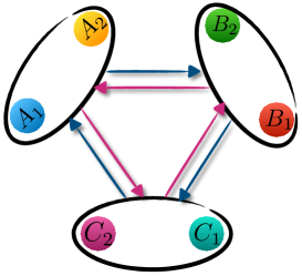
Figure 4: Schematic diagram of the arrangement of Alice’s ($A_{1},\leavevmode\nobreak\ A_{2}$), Bob’s ($B_{1},\leavevmode\nobreak\ B_{2}$), and Charlie’s ($C_{1},\leavevmode\nobreak\ C_{2}$) quantum systems in the three-party causal order game. Each arrow connects a pair of parties such that the start point of the arrow indicates the party that will generate the random bit ($a$ or $b$ or c). Whereas, the end point of the arrow indicates the party that will produce a guess bit ($x$ or $y$ or $z$) of that random bit.

V Generalization to higher parties

In this section, we provide a methodology to generalize the causal order game presented above for a higher number of parties keeping the set-up compatible with the quantum many-body Hamiltonian that we consider in our work. In particular, we generalize the above game for three parties ($N=6$) and derive the corresponding classical and quantum bound of the success probabilities. This methodology could be useful to extend the game for any number of parties. Consider the game now consists of three parties Alice, Bob, and Charlie with their input and output systems denoted by $(A_{1},A_{2}),(B_{1},B_{2})$, and $(C_{1},C_{2})$, respectively. Additionally, we consider Alice is the left neighbor of Bob and the right neighbor of Charlie. Similarly Bob is the left neighbor of Charlie and the right neighbor of Alice. Finally, Charlie is the left neighbor of Alice and the right neighbor of Bob. Moreover, similar to the two-player game, the random bit generated by the parties can be denoted as $a$ (for Alice), $b$ (for Bob), and $c$ (for Charlie). Each of the parties now has to guess the random bit of the other two parties (see schematic presented in Fig. 4) and they will do that following the value of an additional random bit ‘$b^{\prime}$’ that will be generated by an external agent Crupier: if $b^{\prime}=0$, the parties has to guess the bit of their left neighbor. Whereas, if $b^{\prime}=1$, each of the party will guess the bit of its right neighbor. Now if we denote the guess bits produced by all the parties as $x$ (for Alice), $y$ (for Bob), and $z$ (for Charlie), the task will be to maximize the probability function given by

$$P_{success} = \frac{1}{2}\Big{[}P^{Left}_{success}+P^{Right}_{success}\Big{]},$$ (14)

with

$$P_{success}^{Left}(b^{\prime}=0) = \frac{1}{3}\Big{[}P_{Alice}(x=c)+P_{Bob}(y=a)$$ (15)

$$+ P_{Charlie}(z=b)\Big{]},$$

$$P_{success}^{Right}(b^{\prime}=1) = \frac{1}{3}\Big{[}P_{Alice}(x=b)+P_{Bob}(y=c)$$ (16)

$$+ P_{Charlie}(z=a)\Big{]}.$$

Now let us consider there exist a global causal order such as $A\preceq B\preceq C$. In that case, one can show that $P_{success}$ is bounded above by $3/4$. This can be proved as follows. As Alice is in the causal past of both Bob and Charlie, Alice can guess their bits with maximum probability $P_{Alice}(x=b)=P_{Alice}(x=c)=\frac{1}{2}$. Whereas, Bob is in the causal past of Charlie and in the future of Alice. Hence, with the help of Alice, Bob can guess her bit perfectly but can only guess the bit of Charlie, randomly. Hence, we get $P_{Bob}(y=a)=1$, and $P_{Bob}(y=c)=\frac{1}{2}$. However, Charlie remains in the causal future of both Alice and Bob. Hence, he can guess their bits perfectly $P_{Charlie}(z=a)=P_{Charlie}(z=b)=1$. Therefore, we finally get

$$P^{Right}_{success} = \frac{1}{3}\Big{[}\frac{1}{2}+\frac{1}{2}+1]=\frac{2}{3},P^{Left}_{success}=\frac{1}{3}\Big{[}\frac{1}{2}+1+1\Big{]}=\frac{5}{6},$$

which yields $P_{success}=\frac{3}{4}$.

To formulate a quantum version, we take the following process matrix

$$W(\theta)=\frac{1}{8}\Big{[}\mathbb{I}+\frac{f_{0}(\theta,\leavevmode\nobreak\ N=6)}{3}(\sigma_{z}^{A_{2}}\sigma_{z}^{B_{1}}+\sigma_{z}^{B_{2}}\sigma_{z}^{C_{1}}+\sigma_{z}^{A_{1}}\sigma_{z}^{C_{2}})$$

$$+ \frac{f_{1}(\theta,\leavevmode\nobreak\ N=6)}{3}(\sigma_{x}^{A_{1}}\sigma_{x}^{B_{1}}\sigma_{z}^{B_{2}}+\sigma_{x}^{B_{1}}\sigma_{x}^{C_{1}}\sigma_{z}^{C_{2}}+\sigma_{x}^{A_{1}}\sigma_{z}^{A_{2}}\sigma_{x}^{C_{1}})\Big{]},$$

where the meaning of the functions $f_{0}(\theta,\leavevmode\nobreak\ N=6)$ and $f_{1}(\theta,\leavevmode\nobreak\ N=6)$ will be clear when we introduce corresponding quantum many-body Hamiltonian. Let us now consider the measurement operators for input and output systems of each of the parties that can be expressed as

$${\mathcal{P}}^{\chi_{1}\chi_{2}}_{b^{\prime}}(\alpha,\beta;\zeta) = \frac{1}{2}(\mathbb{I}^{\chi_{1}}+(-1)^{\alpha}\sigma_{\zeta}^{\chi_{1}})\frac{1}{2}(\mathbb{I}^{\chi_{2}}+(-1)^{\beta}\sigma_{z}^{\chi_{2}}),$$

where $\chi\in A,B,C$, and $\zeta\in x,y,z$. The quantum measurement operators for each parties for a certain value of $b^{\prime}$ and the probabilities are summarized in Table 2. The total projector ${\mathcal{P}}^{A_{1}A_{2}B_{1}B_{2}C_{1}C_{2}}_{b^{\prime}}(\alpha,\beta;\zeta)$ is the product of the individual $\mathcal{P}$’s given in the table.

$b^{\prime}$	$A$	$B$	$C$	$Probability$
0	$\begin{array}[]{lcl}{\mathcal{P}}^{A_{1}A_{2}}_{b^{\prime}=0}(x,0;z)\end{array}$	$\begin{array}[]{lcl}{\mathcal{P}}^{B_{1}B_{2}}_{b^{\prime}=0}(0,0;z)\end{array}$	$\begin{array}[]{lcl}{\mathcal{P}}^{C_{1}C_{2}}_{b^{\prime}=0}(0,c;z)\end{array}$	$\begin{array}[]{lcl}P_{Alice}(x=c,b^{\prime}=0)=\frac{1+f_{0}((\theta,\leavevmode\nobreak\ N=6)}{2}\end{array}$
0	$\begin{array}[]{lcl}{\mathcal{P}}^{A_{1}A_{2}}_{b^{\prime}=0}(0,a;z)\end{array}$	$\begin{array}[]{lcl}{\mathcal{P}}^{B_{1}B_{2}}_{b^{\prime}=0}(y,0;z)\end{array}$	$\begin{array}[]{lcl}{\mathcal{P}}^{C_{1}C_{2}}_{b^{\prime}=0}(0,0;z)\end{array}$	$\begin{array}[]{lcl}P_{Bob}(y=a,b^{\prime}=0)=\frac{1+f_{0}(\theta,\leavevmode\nobreak\ N=6)}{2}\end{array}$
0	$\begin{array}[]{lcl}{\mathcal{P}}^{A_{1}A_{2}}_{b^{\prime}=0}(0,0;z)\end{array}$	$\begin{array}[]{lcl}{\mathcal{P}}^{B_{1}B_{2}}_{b^{\prime}=0}(0,b;z)\end{array}$	$\begin{array}[]{lcl}{\mathcal{P}}^{C_{1}C_{2}}_{b^{\prime}=0}(z,0;z)\end{array}$	$\begin{array}[]{lcl}P_{Charlie}(z=b,b^{\prime}=0)=\frac{1+f_{0}(\theta,\leavevmode\nobreak\ N=6)}{2}\end{array}$
1	$\begin{array}[]{lcl}{\mathcal{P}}^{A_{1}A_{2}}_{b^{\prime}=1}(x,x;x)\end{array}$	$\begin{array}[]{lcl}{\mathcal{P}}^{B_{1}B_{2}}_{b^{\prime}=1}(0,b;x)\end{array}$	$\begin{array}[]{lcl}{\mathcal{P}}^{C_{1}C_{2}}_{b^{\prime}=1}(0,0;x)\end{array}$	$\begin{array}[]{lcl}P_{Alice}(x=b,b^{\prime}=1)=\frac{1+f_{1}(\theta,\leavevmode\nobreak\ N=6)}{2}\end{array}$
1	$\begin{array}[]{lcl}{\mathcal{P}}^{A_{1}A_{2}}_{b^{\prime}=1}(0,0;x)\end{array}$	$\begin{array}[]{lcl}{\mathcal{P}}^{B_{1}B_{2}}_{b^{\prime}=1}(y,y;x)\end{array}$	$\begin{array}[]{lcl}{\mathcal{P}}^{C_{1}C_{2}}_{b^{\prime}=1}(0,c;x)\end{array}$	$\begin{array}[]{lcl}P_{Bob}(y=c,b^{\prime}=1)=\frac{1+f_{1}(\theta,\leavevmode\nobreak\ N=6)}{2}\end{array}$
1	$\begin{array}[]{lcl}{\mathcal{P}}^{A_{1}A_{2}}_{b^{\prime}=1}(0,a;x)\end{array}$	$\begin{array}[]{lcl}{\mathcal{P}}^{B_{1}B_{2}}_{b^{\prime}=1}(0,0;x)\end{array}$	$\begin{array}[]{lcl}{\mathcal{P}}^{C_{1}C_{2}}_{b^{\prime}=1}(z,z;x)\end{array}$	$\begin{array}[]{lcl}P_{Charlie}(z=a,b^{\prime}=1)=\frac{1+f_{1}(\theta,\leavevmode\nobreak\ N=6)}{2}\end{array}$

Table 2: List of quantum measurement operators ${\mathcal{P}}^{A_{1}A_{2}}_{b^{\prime}}(\alpha,\beta;\zeta)$, ${\mathcal{P}}^{B_{1}B_{2}}_{b^{\prime}}(\alpha,\beta;\zeta)$, ${\mathcal{P}}^{C_{1}C_{2}}_{b^{\prime}}(\alpha,\beta;\zeta)$ applied on the process matrix $W$ expressed in Eq. (LABEL:eqn:process_three_party) for each strategy ($b^{\prime}$) which finally yields $P^{Left}_{success}=\frac{1+f_{0}(\theta,\leavevmode\nobreak\ N=6)}{2}$ and $P^{Right}_{success}=\frac{1+f_{1}(\theta,\leavevmode\nobreak\ N=6)}{2}$. Hence, we get $P_{success}=\frac{P^{Left}_{success}+P^{Right}_{success}}{2}=\frac{2+f_{0}(\theta,\leavevmode\nobreak\ N=6)+f_{1}(\theta,\leavevmode\nobreak\ N=6)}{4}$.

By exploiting those strategies on the process matrix $W$ expressed in Eq. (LABEL:eqn:process_three_party), we find

$$P^{Left}_{success} = \frac{1+f_{0}(\theta,\leavevmode\nobreak\ N=6)}{2},\leavevmode\nobreak\ P^{Right}_{success}=\frac{1+f_{1}(\theta,\leavevmode\nobreak\ N=6)}{2}.$$

Using this we finally get

$$P_{success} = \frac{P^{Left}_{success}+P^{Right}_{success}}{2}$$

$$= \frac{2+f_{0}(\theta,\leavevmode\nobreak\ N=6)+f_{1}(\theta,\leavevmode\nobreak\ N=6)}{4}.$$

However, we would like to mention that the process matrix we consider in Eq. (LABEL:eqn:process_three_party) is not the optimal one. It has been shown in Ref. causal_order_three_parties that there exist a process matrix and a set of measurements for which one can get the maximum value of the total success probability to be 1, which is higher than the value obtained for the two-player game. Hence, one can think that in some sense the proposed three-party causal order game is analogous to the nonlocal game with the GHZ state GHZ1 ; GHZ2 . As similar to the maximal violation of causal order obtained in this case, in the GHZ game, the violation of locality is maximal. In our case, we do not consider such a process matrix as it is structurally very different from the quantum many-body Hamiltonian we consider in our work. The $W$ matrix considered in Ref. causal_order_three_parties consists of four and five body terms while in our game to make it consistent with the quantum many-body Hamiltonian, the operators involved in $W$ are only two and three-body.

Therefore, we argue that the original causal order game can be extended to a multi-player game consisting of $\mathcal{N}=N/2$ parties ($\mathcal{S}_{1},\mathcal{S}_{2},\dots,\mathcal{S}_{\mathcal{N}}$) such that if we arrange the parties in a clockwise cyclic pattern according to ascending order of their index, each of them has to guess the random classical bits of their immediate neighbors. We call $\mathcal{S}_{i}$ is the left neighbor of $\mathcal{S}_{i+1}$ and the right neighbor of $\mathcal{S}_{i-1}$, with boundary conditions $\mathcal{S}_{0}=\mathcal{S}_{\mathcal{N}}$ and $\mathcal{S}_{\mathcal{N}+1}=\mathcal{S}_{1}$. If Crupier provides $b^{\prime}=0$, everyone needs to guess the bit of their left neighbor ($P^{Left}_{\mathcal{S}_{i}}$) and $P^{Left}_{success}(b^{\prime}=0)$ is just the average of the left probability computed for each party, i.e., $P^{Left}_{success}(b^{\prime}=0)=\frac{1}{\mathcal{N}}\sum_{i=1}^{\mathcal{N}}P^{Left}_{\mathcal{S}_{i}}$. Similarly when $b^{\prime}=1$, the parties need to guess the random bit of their right neighbor ($P^{Right}_{\mathcal{S}_{i}}$) which will estimate $P^{Right}_{success}(b^{\prime}=1)=\frac{1}{\mathcal{N}}\sum_{i=1}^{\mathcal{N}}P^{Right}_{\mathcal{S}_{i}}$. Now same as before, we consider a definite causal ordering between the parties, such that $\mathcal{S}_{1}\preceq\mathcal{S}_{2}\preceq\mathcal{S}_{3}\preceq\dots\preceq\mathcal{S}_{\mathcal{N}}$. As a result, we find that for $(\mathcal{N}-2)$ parties ($\mathcal{S}_{2}$ to $\mathcal{S}_{\mathcal{N}-1}$), the neighbor in the left remains in the causal past and thus they can guess its bit perfectly. Whereas, the other neighbor is in their causal future. Hence, they can only guess its classical bit randomly. Therefore, together they contribute factors $\frac{\mathcal{N}-2}{\mathcal{N}}$ and $\frac{\mathcal{N}-2}{2\mathcal{N}}$ to $P^{Left}_{success}(b^{\prime}=0)$ and $P^{Right}_{success}(b^{\prime}=1)$, respectively. However, if we consider $\mathcal{S}_{1}$, both of its neighbors remain in its causal future. Hence, it can only guess their bits randomly that yields $P_{\mathcal{S}_{1}}^{Left}=P_{\mathcal{S}_{1}}^{Right}=\frac{1}{2}$. Similarly, $\mathcal{S}_{\mathcal{N}}$ remains in the causal future of its both neighbors and can guess their bits exactly, that yields $P_{\mathcal{S}_{\mathcal{N}}}^{Left}=P_{\mathcal{S}_{\mathcal{N}}}^{Right}=1$. Therefore, we finally get

$$P^{Left}_{success}(b^{\prime}=0) = 1-\frac{1}{2\mathcal{N}},\leavevmode\nobreak\ \text{and}\leavevmode\nobreak\ P^{Right}_{success}(b^{\prime}=1)=\frac{1}{2}+\frac{1}{2\mathcal{N}}.$$

Hence, the total success probability of the classical game is again $P_{success}^{classical}=\frac{1}{2}\Big{(}P^{Left}_{success}(b^{\prime}=0)+P^{Right}_{success}(b^{\prime}=1)\Big{)}=\frac{3}{4}$.

In the quantum version of the $\mathcal{N}$-party game, we want the success probabilities to take the values similar to those derived in Eqs. (LABEL:en:success:new)-(LABEL:eqn:success:three_party), given by

$$P^{Left}_{success} = \frac{1+f_{0}(\theta,\leavevmode\nobreak\ N)}{2},\leavevmode\nobreak\ P^{Right}_{success}=\frac{1+f_{1}(\theta,\leavevmode\nobreak\ N)}{2},$$ (23)

and thus yielding

$$P_{success} = \frac{P^{Left}_{success}+P^{Right}_{success}}{2}=\frac{2+f_{0}(\theta,\leavevmode\nobreak\ N)+f_{1}(\theta,\leavevmode\nobreak\ N)}{4}.$$

We argue that the above probabilities can be obtained by exploiting appropriate measurement strategy on an $\mathcal{N}$-party process matrix with the general form given by

$$W(\theta) = \frac{1}{2^{\mathcal{N}}}\Big{[}\mathbb{I}+\frac{f_{0}(\theta,\leavevmode\nobreak\ N)}{\mathcal{N}_{0}}\Big{(}\sum_{i=1}^{\mathcal{N}_{0}}\sigma_{\alpha}^{\mathcal{S}_{i}^{O}}\sigma_{\beta}^{\mathcal{S}_{i+1}^{I}}\Big{)}$$

$$+ \frac{f_{1}(\theta,\leavevmode\nobreak\ N)}{\mathcal{N}_{1}}\Big{(}\sum_{i=1}^{\mathcal{N}_{1}}\sigma_{\gamma}^{\mathcal{S}_{i}^{I}}\sigma_{\delta}^{\mathcal{S}_{i+1}^{I}}\sigma_{\eta}^{\mathcal{S}^{O}_{i+1}}\Big{)}\Big{]},$$

where $\mathcal{N}_{0}$ ($\mathcal{N}_{1}$) is the number of two-body (three-body) terms in $W$, $\mathcal{S}_{i}^{I}$ ($\mathcal{S}_{i}^{O}$) is the input (output) quantum system of the $i^{th}$ party. Whereas, $\alpha,\beta,\gamma,\delta,\eta\in\{x,y,z\}$ and their choices depend on certain factors, e.g., number of parties, validity of $W$ as a process matrix, etc. For example, for $N=6$ ($\mathcal{N}=3$), we choose $\alpha=\beta=\eta=z$, $\gamma=\delta=x$ and $\mathcal{N}_{0}=\mathcal{N}_{1}=3$.

To establish a correspondence of this generalized game with a suitable quantum many-body system, we consider a quantum many-body Hamiltonian similar to the previous one that includes an Ising interaction and a cluster Hamiltonian, expressed as

$$\mathcal{H}(\theta)=-\cos\theta\sum_{i=1}^{N}\sigma_{z}^{i}\sigma_{z}^{i+2}-\sin\theta\sum_{i=1}^{N}\sigma_{z}^{i}\sigma_{x}^{i+1}\sigma_{z}^{i+2},$$ (26)

where PBC are enforced. One can note that for $N>4$, the number of terms present in the Ising part and the cluster part is the same. Hence, we no longer need the factor 2 in front of the Ising part. The Hamiltonian can be solved exactly ref_new1 ; ref_new2 by first mapping it to two transverse field Ising models using the controlled-phase ($\mathcal{CZ}$) operation on pair of sites, given by

$$\mathcal{U}=\Pi_{i}\mathcal{CZ}_{i,i+1},\text{with}\hskip 2.84544pt\mathcal{CZ}_{i,i+1}=|0\rangle\langle 0|^{i}\otimes\mathbb{I}^{i+1}+|1\rangle\langle 1|^{i}\otimes\sigma_{z}^{i+1},$$

(27)

which yields

$$\mathcal{U}\mathcal{H}\mathcal{U}^{\dagger}=\mathcal{H}_{\text{TFIM}}^{odd}+\mathcal{H}_{\text{TFIM}}^{even},$$ (28)

where $\mathcal{H}^{odd}_{\text{TFIM}}$ and $\mathcal{H}^{even}_{\text{TFIM}}$ are the nearest-neighbor transverse field Ising model (TFIM) on odd and even sites respectively, defined as

$$\mathcal{H}^{odd}_{\text{TFIM}} = -\cos\theta\sum_{i=1}^{N/2}\sigma_{z}^{2i-1}\sigma_{z}^{2i+1}-\sin\theta\sum_{i=1}^{N/2}\sigma_{x}^{2i-1},$$

$$\mathcal{H}^{even}_{\text{TFIM}} = -\cos\theta\sum_{i=1}^{N/2}\sigma_{z}^{2i}\sigma_{z}^{2(i+1)}-\sin\theta\sum_{i=1}^{N/2}\sigma_{x}^{2i}.$$ (29)

Each of the above TFIMs can be solved exactly by mapping it to a free-fermionic model using Jordan-Wigner transformation JW (see Appendix A). Therefore, the transformation not only helps us to solve the model Hamiltonian given in Eq. (26) explicitly, it also relates the model to one with well-understood quantum phases and order parameters. Now as these two TFIMs of equal length do not interact with each other, it is enough to diagonalize one of them and compute the relevant physical quantities of the actual model out of that. Hence, from now onwards, we only consider one of them with the general form

$$\mathcal{H}_{\text{TFIM}} = -\cos\theta\sum_{i=1}^{N/2}\sigma_{z}^{i}\sigma_{z}^{i+1}-\sin\theta\sum_{i=1}^{N/2}\sigma_{x}^{i},$$ (30)

and let us denote the GS of this model by $|\Phi\rangle_{g}$. Moreover, under the unitary operation defined in Eq. (27) the projector in Eq. (11) changes as

$$\Pi^{0}=\frac{1}{2}\big{(}\mathbb{I}^{i\leavevmode\nobreak\ i+1\leavevmode\nobreak\ i+2}+\sigma_{z}^{i}\sigma_{x}^{i+1}\sigma_{z}^{i+2}\big{)} \rightarrow \mathcal{U}\Pi^{0}\mathcal{U}^{\dagger}=\frac{1}{2}\big{(}\mathbb{I}^{i+1}+\sigma^{i+1}_{x}),$$

$$\Pi^{1}=\frac{1}{2}\big{(}\mathbb{I}^{i\leavevmode\nobreak\ i+2}+\sigma_{z}^{i}\sigma_{z}^{i+2}\big{)} \rightarrow \mathcal{U}\Pi^{1}\mathcal{U}^{\dagger}=\Pi^{1}.$$ (31)

Hence, the exact solution of the TFIMs provides a close analytical form of all the above quantities for any arbitrary system size $N$.

We now consider that the expectation value of the two-body and the three-body operators are equal to the functions $f_{i}(\theta,N)$ introduced in Eq. (LABEL:eqn:process_N_party), i.e.,

$$f_{0}(\theta,\leavevmode\nobreak\ N) = C_{zz}={{}_{g}}\langle\Phi|\sigma_{z}^{i}\sigma_{z}^{i+2}|\Phi\rangle_{g},$$

$$f_{1}(\theta,\leavevmode\nobreak\ N) = m_{x}={{}_{g}}\langle\Phi|\sigma_{x}^{i}|\Phi\rangle_{g}.$$ (32)

This again provides us with the scope to relate the success probabilities obtained for the $\mathcal{N}$-party causal order game with that of the expectation values of the projectors computed for the GS of the quantum many-body Hamiltonian of the size $N=2\mathcal{N}$. In other words, we get from Eqs. (LABEL:en:success:new)-(LABEL:eqn:success:three_party)

$$P_{success}^{Left}=\frac{1+C_{zz}}{2},P_{success}^{Right}=\frac{1+m_{x}}{2}.$$

(33)

Hence, the total success probability of the game can again be related with the average of the expectation values of the projectors ($\mathcal{K}_{avg}$), as introduced in Eq. (12),

$$\mathcal{K}_{avg}\equiv P_{success}=\frac{2+m_{x}+C_{zz}}{4}.$$

We plot the behavior of $\mathcal{K}_{avg}$ ($P_{success}$) in Fig. 5 for different system sizes. One can note that similar to $N=4$ case, $\mathcal{K}_{avg}$ ($P_{success}$) becomes maximum at $\theta_{c}=\frac{\pi}{4}$ for all values of $N$. Hence, the correspondence observed for $N=4$ equally holds for large system size: maximum violation of the causality corresponds to a second-order QPT in the considered quantum many-body model.

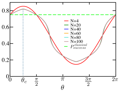
Figure 5: Plot of scaling of success probability of the $\mathcal{N}$-party causal order game with the process matrix defined in Eq. (LABEL:eqn:process_N_party) or equivalently $\mathcal{K}_{avg}$ computed for the GS of the model defined in Eq. (26) (for $N>4$ and Eq. (1) for $N=4$). The plot for system size $N=4$ is denoted by broken red curve. Whereas, all the remaining plots (i.e., for $N=20,40,80,100$) are denoted by solid curves. One can note that the plots for $N\geq 20$ become indistinguishable from each other. Moreover, similar to $N=4$ case, all of them attain maxima at $\theta_{c}=\frac{\pi}{4}$. The horizontal broken straight line has the same meaning as in Fig. 2

.

VI Detection OF quantum phase transition point

In this section, we provide a detailed discussion about efficient detection of the QPT point in the model Hamiltonian defined in Eq. (26). For that purpose, we first seek suitable order parameters characterizing the Ising and the cluster phases of the model and analyze their behavior with the parameter $\theta$. Note that for our analysis, it is enough to choose the region of interest as $0\leq\theta\leq\frac{\pi}{2}$. From Eq. (30), we can see for the Ising phase, a suitable order parameter is the longitudinal magnetic field $m_{z}={{}_{g}}\langle\Phi|\sigma^{i}_{z}|\Phi\rangle_{g}$ which remains non-zero only for the region $0\leq\theta<\frac{\pi}{4}$. In the thermodynamic limit, $m_{z}$ behaves as pfeuty

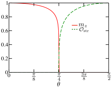
Figure 6: Plot of the behavior of the order parameters characterizing the Ising phase, $m_{z}$ (solid red line) and the cluster phase, $\mathcal{O}_{\text{str}}$ (broken green line) defined in Eq. (36) as a function of $\theta$. $m_{z}$ remains non-zero for the region $0\leq\theta<\frac{\pi}{4}$ and decays following Eq. (35). Whereas, $\mathcal{O}_{\text{str}}$ exhbits completely opposite behavior and has non-zero value only for the region $\frac{\pi}{4}<\theta\leq\frac{\pi}{2}$ where it decays following Eq. (42).

$$m_{z}=\begin{cases}(1-\tan^{2}\theta)^{1/8}&\text{for $0\leq\theta<\frac{\pi}{4}$},\\ 0&\text{for $\frac{\pi}{4}<\theta\leq\frac{\pi}{2}$.}\end{cases}$$ (35)

On the other hand, for the cluster phase we choose the following string order parameter that characterizes hidden antiferromagnetic order of the model, defined as SOP1 ; pollmann

$$\mathcal{O}_{\text{str}} = {{}_{g}}\langle\Psi|\Pi_{i=1}^{N}\sigma_{x}^{i}|\Psi\rangle_{g}.$$ (36)

Now it is easy to see that $\Pi_{i=1}^{N}\sigma_{x}^{i}$ remains invariant under the transformation given in Eq. (27), i.e.,

$$\mathcal{U}\Pi_{i=1}^{N}\sigma_{x}^{i}\mathcal{U}^{\dagger}=\Pi_{i=1}^{N}\sigma_{x}^{i}.$$ (37)

Hence, to compute the value of $\mathcal{O}_{\text{str}}$ for the GS of the TFIM we need to consider the same string of operators,

$$\mathcal{O}_{\text{str}} = \Big{[}{{}_{g}}\langle\Phi|\Pi_{i=1}^{N/2}\sigma_{x}^{i}|\Phi\rangle_{g}\Big{]}^{2}.$$ (38)

Moreover, using the Kramers-Wannier duality transformation Kramers ,

$$\mu^{i}_{z}=\Pi_{j=1}^{i}\sigma^{j}_{x},\hskip 5.69046pt\mu^{i}_{x}=\sigma^{i}_{z}\sigma^{i+1}_{z},$$ (39)

one can define a dual Hamiltonian to the TFIM model expressed in Eq. (30) and get

$$H_{\text{TFIM}}^{dual}=-\sin\theta\sum_{i=1}^{N/2}\mu_{z}^{i}\mu^{i+1}_{z}-\cos\theta\sum_{i=1}^{N/2}\mu_{x}^{i}.$$ (40)

This suggests, computation of the string operator $\Pi_{i=1}^{N/2}\sigma_{x}^{i}$ for the GS of the TFIM defined in Eq. (30) is equivalent to computation of the longitudinal magnetization ($\langle\mu^{N/2}_{z}\rangle$) for the GS of the dual Hamiltonian $H_{\text{TFIM}}^{dual}$. In other words,

$$\mathcal{O}_{\text{str}} = \Big{[}{{}_{g}}\langle\Phi^{dual}|\mu_{z}^{N/2}|\Phi^{dual}\rangle_{g}\Big{]}^{2},$$ (41)

where we denote $|\Phi^{dual}\rangle_{g}$ as the GS of $H_{\text{TFIM}}^{dual}$. Again, using the analytical form of the longitudinal magnetization in the thermodynamic limit, we get

$$\mathcal{O}_{\text{str}}=\begin{cases}0&\text{for $0\leq\theta<\frac{\pi}{4}$},\\ (1-\cot^{2}\theta)^{1/4}&\text{for $\frac{\pi}{4}<\theta\leq\frac{\pi}{2}$.}\end{cases}$$ (42)

Therefore, from Eqs. (35) and Eqs. (42) one can find that for the considered range of $\theta$ the behavior of these two quantities remain complementary to each other and thus they serve as efficient order parameters characterizing two different phases of the model. We provide a pictorial depiction of the same in Fig. 6 where the QPT point $\theta_{c}=\frac{\pi}{4}$ is marked by the point where both the quantities vanish simultaneously.

We now compare the success probabilities obtained for an $N$-party causal order game with the different phases of the considered Hamiltonian for the region $0\leq\theta\leq\frac{\pi}{2}$. For that purpose, we plot the behavior of the success probabilities ($P_{success}^{Left/Right}$) obtained using Eq. (33) for large value of $N$ in Fig. 7 and compare that with Fig. 6. From the plot, we note that different phases of the model favour different strategies of the game. For instance, for the region $0\leq\theta<\frac{\pi}{4}$ when the system remains in the Ising phase, $P_{success}^{Left}$ dominates over $P_{success}^{Right}$. Similarly, for $\frac{\pi}{4}<\theta\leq\frac{\pi}{2}$ when the system remains in the SPT phase, $P_{success}^{Right}$ becomes higher than $P_{success}^{Left}$. At the QPT point, we get $P_{success}^{Left}=P_{success}^{Right}$ and the total success probability becomes maximum.

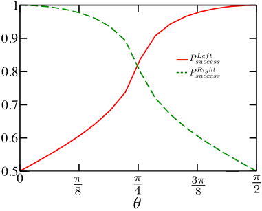
Figure 7: Plot of the probabilities of the causal order game $P_{success}^{Left}$ (broken green line) and $P_{success}^{Right}$ (solid red line) which are the functions of the observables $C_{zz}$ and $m_{x}$ respectively (see Eq. (33)), computed for the GS of the TFIM defined in Eq. (30) with $\theta$. Here we consider $N=100$.

VII Discussion and future work

In this work, we have presented a framework to relate the eigenstates of a topological Hamiltonian with the resource of causal order game introduced in Ref. brukner , called the process matrix. In particular, we have shown that the success probabilities of different strategies of the game can be realized as expectation values of different observables computed for the eigenstates of the model. Thus the GS and the most excited state can be related to a non-causally separable process matrix whenever the sum of a certain two-body and three-body correlations exceed a minimum value. However, for other excited states, the process matrix to which they can be related remains causally separable for the whole range of the system parameters. In addition to this, we showed that at the point of maximum violation of the causal order, in the thermodynamic limit corresponding quantum many-body model undergoes a second-order QPT. We further showed that different quantum phases of the model can favor different quantum strategies of the model. For instance, in the Ising phase $P_{success}^{Left}$ remains higher than that of $P_{success}^{Right}$. Whereas, for the cluster phase of the model opposite ordering appeared. The results have been generalized for a higher number of parties and the behavior remains the same. We believe that our work is a genuine attempt to establish a correspondence between quantum many-body systems and quantum game theory which may become useful for experimental realization of the game-theoretic schemes IBM . As future work, we wish to consider a generalized version of the Hamiltonian $\mathcal{H}$ that includes additional non-commutative terms along with long-range interactions and relate that to a modified version of the game.

Appendix A Jordan-Wigner transformation and computation of observables

We start with the nearest-neighbor transverse filed Ising model

$$\mathcal{H}_{\text{TFIM}} = -\cos\theta\sum_{i=1}^{N/2}\sigma_{z}^{i}\sigma_{z}^{i+1}-\sin\theta\sum_{i=1}^{N/2}\sigma_{x}^{i}.$$ (43)

Now let us do the following transformation

$$\sigma_{x}^{i}=2c_{i}^{\dagger}c_{i}-1,\sigma_{z}^{i}=-\Pi_{k<i}(1-2c_{k}^{\dagger}c_{k})(c_{i}+c_{i}^{\dagger}),$$ (44)

where $c_{i}(c_{i}^{\dagger})$ are spinless fermionic anhilation (creation) operator at site $i$. Plugging this in Eq. (43) we get

$$\mathcal{H}_{\text{TFIM}} = -\cos\theta\sum_{i=1}^{N/2}\Big{[}c_{i}^{\dagger}c_{i+1}+c_{i+1}^{\dagger}c_{i}+c_{i}^{\dagger}c_{i+1}^{\dagger}+c_{i+1}c_{i}\Big{]}-\sin\theta\sum_{i=1}^{N/2}(2c_{i}^{\dagger}c_{i}-1),$$ (45)

$$= \sum_{i,j=1}^{N/2}\Big{[}c_{i}^{\dagger}A_{ij}c_{j}+\frac{1}{2}(c_{i}^{\dagger}B_{ij}c_{j}^{\dagger}+c_{i}B_{ij}c_{j})\Big{]},$$ (46)

where $A_{ij}=-\cos\theta(\delta_{j,i+1}+\delta_{i,j+1})-2\sin\theta\delta_{i,j},B_{ij}=-\cos\theta(\delta_{j,i+1}-\delta_{i,j+1})$, with $A_{1N}=A_{N1}=\cos\theta$ and $B_{1N}=-B_{N1}=-\cos\theta$. Now defining following set of vectors $\psi_{k}$ that obey the eigenvalues equations

$$(A+B)(A-B)\psi_{k}^{T}=\Lambda_{k}^{2}\psi_{k}^{T},$$ (47)

and obtaining the corresponding $\phi_{k}$ using

$$\phi_{k}^{T}=\Lambda_{k}^{-1}(A-B)\psi_{k}^{T},$$ (48)

we can define correlation matrix $G_{ij}$ as follows

$$G_{ij}=-\sum_{k}\psi_{ki}\phi_{kj}=(\psi_{k}^{T}\phi_{k})_{ij}.$$ (49)

This finally yields

$$m^{i}_{x}=-G_{i,i},C^{i,i+1}_{zz}=G_{i,i+1}.$$ (50)

One can note that due to translational invariance the RHS of the above equations does not depend on the site index and we can write $m_{x}=m_{x}^{i}$ and $C_{zz}=C_{zz}^{i,i+1}$.

References

- (1) O. Oreshkov, F. Costa, and Č. Brukner, Quantum correlations with no causal order, Nature Communications 3, 1092 (2012).
- (2) J. Eisert, M. Wilkens, and M. Lewenstein, Quantum Games and Quantum Strategies, Phys. Rev. Lett. 83, 3077 (1999).
- (3) D. A. Meyer, Quantum Strategies, Phys. Rev. Lett. 82, 1052 (1999).
- (4) S. C. Benjamin and P. M. Hayden, Multiplayer quantum games, Phys. Rev. A 64, 030301(R) (2001).
- (5) E. F. Galvao, D.Phil. (Ph.D.) thesis, Foundations of quantum theory and quantum information applications, University of Oxford, arXiv:quant-ph/0212124 (quant-ph) (2002).
- (6) A. P. Flitney and D. Abbott, An introduction to quantum game theory, Fluct. Noise Lett. 2, R175 (2002).
- (7) J. Du, Hui Li, X. Xu, M. Shi, J. Wu, X. Zhou, and R. Han Experimental Realization of Quantum Games on a Quantum Computer, Phys. Rev. Lett. 88, 137902 (2002).
- (8) A. P. Flitney and D. Abbott, Advantage of a quantum player over a classical one in quantum games, Proc. R. Soc. Lond. A. 459, 2463 (2003).
- (9) F. Guinea and M. A. Martin-Delgado, Quantum Chinos game: Winning strategies through quantum fluctuations, J. Phys. A 36, L197 (2003).
- (10) T. Ichikawa, I. Tsutsui, and T. Cheon, Quantum game theory based on the Schmidt decomposition J. Phys. A: Math. Theor. 41, 135303 (2008).
- (11) N. Brunner and N. Linden, Connection between Bell nonlocality and Bayesian game theory, Nat. Commun. 4, 2057 (2013).
- (12) A. Li and X. Yong, Entanglement Guarantees Emergence of Cooperation in Quantum Prisoner’s Dilemma Games on Networks, Sci. Rep. 4, 6286 (2014).
- (13) A. Pappa, N. Kumar, T. Lawson, M. Santha, S. Zhang, E. Diamanti, and I. Kerenidis, Nonlocality and Conflicting Interest Games, Phys. Rev. Lett. 114, 020401 (2015).
- (14) J. F. Clauser, M. A. Horne, A. Shimony, and R. A. Holt, Proposed Experiment to Test Local Hidden-Variable Theories, Phys. Rev. Lett. 23, 880 (1969).
- (15) A. Acin, M. L. Almeida, R. Augusiak, and N. Brunner, Guess your neighbour’s input: no quantum advantage but an advantage for quantum theory, in Quantum Theory: Informational Foundations and Foils, Fundamental Theories in Physics 181, eds. G Chiribella and R. W. Spekkens, (Springer, 2016).
- (16) J. K. Pachos and M. B. Plenio, Three-Spin Interactions in Optical Lattices and Criticality in Cluster Hamiltonians, Phys. Rev. Lett. 93, 056402 (2004).
- (17) W. Son, L. Amico, and V. Vedral, Topological order in 1D Cluster state protected by symmetry, Quantum Inf. Pro. 11, 1961 (2012).
- (18) G. Chiribella, G. M. D’Ariano, P. Perinotti, and B. Valiron, Quantum computations without definite causal structure, Phys. Rev. A 88, 022318 (2013).
- (19) A. Feix, M. Araújo, and Č. Brukner, Quantum superposition of the order of parties as a communication resource, Phys. Rev. A 92, 052326 (2015).
- (20) C. Branciard, Witnesses of causal nonseparability: an introduction and a few case studies, Sci. Rep. 6, 26018 (2016).
- (21) G. Rubino, L. A. Rozema, A. Feix, M. Araújo, J. M. Zeuner, L. M. Procopio, Č. Brukner, and P. Walther, Experimental Verification of an Indefinite Causal Order, Sci. Adv. 3, e1602589 (2017).
- (22) D. Ebler, S. Salek, and G. Chiribella, Enhanced communication with the assistance of indefinite causal order, Phys. Rev. Lett. 120, 1205020 (2018).
-
(23)
A process matrix is a positive semidefinite operator that acts on the tensor product of the input and output Hilbert spaces of Alice and Bob. The set of conditions required for a matrix to be a valid process matrix for the cases are given by
where is the dimension of the output system, i.e., dim() and the operator denotes the CPTP map that can be realized as tracing out the subsystem and replacing it by the normalized identity operator, defined as , with . The notion of process matrix is a generalization of the concept of quantum state. When we discard the output systems ( and ), reduces to a valid density matrix characterizing a quantum system.(51) - (24) Ä. Baumeler and S. Wolf, Perfect signaling among three parties violating predefined causal order, Proc. Int. Symp. Inf. Theory-(ISIT), 526 (2014).
- (25) N. D. Mermin, Quantum mysteries revisited, Am. J. Phys., 58, 731 (1990).
- (26) D. M. Greenberger, M. A. Horne, A. Shimony, and A. Zeilinger, Bell’s theorem without inequalities, Am. J. Phys., 58, 1131, 1990.
- (27) A. C. Doherty and S. D. Bartlett, Identifying Phases of Quantum Many-Body Systems That Are Universal for Quantum Computation, Phys. Rev. Lett. 103, 020506 (2009).
- (28) N. G. Jones, J. Bibo, B. Jobst, F. Pollmann, A. Smith, and R. Verresen, Skeleton of matrix-product-state-solvable models connecting topological phases of matter, Phys. Rev. Research 3, 033265 (2021).
- (29) E. Lieb, T. Schultz, and D. Mattis, Two soluble models of an antiferromagnetic chain, Ann. Phys. 16, 407 (1961).
- (30) P. Pfeuty, The One-Dimensional king Model with a Transverse Field, Annals of Physics. 57, 79 (1970)
- (31) M. den Nijs and K. Rommelse, Preroughening transitions in crystal surfaces and valence-bond phases in quantum spin chains, Phys. Rev. B 40, 4709 (1989).
- (32) A. Smith, B. Jobst, A. G. Green, and F. Pollmann, Crossing a topological phase transition with a quantum computer, arXiv:1910.05351 [cond-mat.str-el] (2019).
- (33) H. A. Kramers and G. H. Wannier, Statistics of the Two-Dimensional Ferromagnet. Part I, Phys. Rev. 60, 252 (1941).
- (34) K. Choo, Curt W. von Keyserlingk, N. Regnault, and T. Neupert, Measurement of the entanglement spectrum of a symmetry-protected topological state using the IBM quantum computer, Phys. Rev. Lett. 121, 086808 (2018).