Objective-aware Traffic Simulation via Inverse Reinforcement Learning

Abstract

Traffic simulators act as an essential component in the operating and planning of transportation systems. Conventional traffic simulators usually employ a calibrated physical car-following model to describe vehicles’ behaviors and their interactions with traffic environment. However, there is no universal physical model that can accurately predict the pattern of vehicle’s behaviors in different situations. A fixed physical model tends to be less effective in a complicated environment given the non-stationary nature of traffic dynamics. In this paper, we formulate traffic simulation as an inverse reinforcement learning problem, and propose a parameter sharing adversarial inverse reinforcement learning model for dynamics-robust simulation learning. Our proposed model is able to imitate a vehicle’s trajectories in the real world while simultaneously recovering the reward function that reveals the vehicle’s true objective which is invariant to different dynamics. Extensive experiments on synthetic and real-world datasets show the superior performance of our approach compared to state-of-the-art methods and its robustness to variant dynamics of traffic.

1 Introduction

Traffic simulation has long been one of the significant topics in transportation. Microscopic traffic simulation plays an important role in planing, designing and operating of transportation systems. For instance, an elaborately designed traffic simulator allows the city operators and planers to test policies of urban road planning, traffic restrictions, and the optimization of traffic congestion, by accurately deducing possible effects of the applied policies to the urban traffic environment  Toledo et al. (2003). The prior work Wei et al. (2018) employs a traffic simulator to train and test policies of intelligent traffic signal control, as it can generate a large number of simulated data for the training of the signal controller.

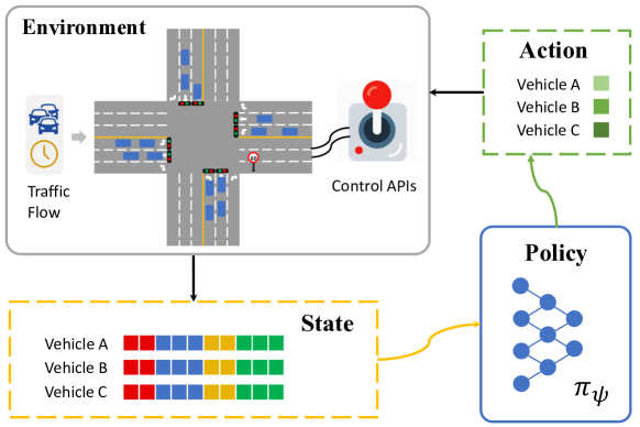
Figure 1: Interactions between the simulation environment and policy (e.g., car-following model).

Current transportation approaches used in the state-of-the-art traffic simulators such as Yu and Fan (2017); Osorio and Punzo (2019) employ several physical and empirical equations to describe the kinetic movement of individual vehicles, referred to as the car-following model (CFM). The parameters of CFMs such as max acceleration and driver reaction time must be carefully calibrated using traffic data. A calibrated CFM can be exploited as a policy providing the vehicle optimal actions given the state of the environment, as shown in Figure 1. The optimality of this policy is enabled by the parameter calibration that obtains a close match between the observed and simulated traffic measurements.

An effective traffic simulator should produce accurate simulations despite variant dynamics in different traffic environment. This can be factorized into two specific objectives. The first objective is to accurately imitate expert vehicle behaviors given a certain environment with stationary dynamics. The movement of real-world vehicles depends on many factors including speed, distance to neighbors, road networks, traffic lights, and also driver’s psychological factors. A CFM usually aims to imitate the car-following behavior by applying physical laws and human knowledge in the prediction of vehicle movement. Faced with sophisticated environment, models with emphasis on fitting different factors are continuously added to the CFM family. For example, Krauss model Krauß (1998) focuses on safety distance and speed, while Fritzsche model sets thresholds for vehicle’s movement according to driver’s psychological tendency. However, there is no universal model that can fully uncover the truth of vehicle-behavior patterns under comprehensive situations. Relying on inaccurate prior knowledge, despite calibrated, CFMs often fail to exhibit realistic simulations.

The second objective is to make the model robust to variant dynamics in different traffic environment. However, it is challenging due to the non-stationary nature of real-world traffic dynamics. For instance, weather shifts and variances of road conditions may change a vehicle’s mechanical property and friction coefficient against the road surface, and eventually lead to variances of its acceleration and braking performance. In a real-world scenario, a vehicle would accordingly adjust its driving policy and behave differently (e.g., use different acceleration or speed given the same observation) under these dynamics changes. However, given a fixed policy (i.e., CFM), current simulators in general, fail to adapt policies to different dynamics. To simulate a different traffic environment with significantly different dynamics, the CFM must be re-calibrated using new trajectory data with respect to that environment, which is inefficient and sometimes unpractical. This makes these simulation models less effective when generalized to changed dynamics.

We aim to achieve both objectives. For the first objective, a natural consideration is to learn patterns of vehicles’ behaviors directly from real-world observations, instead of relying on sometimes unreliable prior knowledge. Recently, imitation learning (IL) has shown promise for learning from demonstrations Ho and Ermon (2016); Fu et al. (2018). However, direct IL methods such as behavioral cloning Michie et al. (1990) that aim to directly extract an expert policy from data, would still fail in the second objective, as the learned policy may lose optimality when traffic dynamics change. A variant of IL, inverse reinforcement learning (IRL), different from direct IL, not only learns an expert’s policy, but also infers the reward function (i.e., cost function or objective) from demonstrations. The learned reward function can help explain an expert’s behavior and give the agent an objective to take actions imitating the expert, which enables IRL to be more interpretable than direct IL. To this end, we propose to use an IRL-based method that build off the adversarial IRL (AIRL) Fu et al. (2018), to train traffic simulating agents that both generate accurate trajectories while simultaneously recovering the invariant underlying reward of the agents, which facilitates the robustness to variant dynamics.

With disentangled reward of an agent recovered from real-world demonstrations, we can infer the vehicle’s true objective. Similar to the human driver’s intention (e.g., drive efficiently under safe conditions), the estimated objective can be invariant to changing dynamics (e.g., maximum acceleration or deceleration). Considering the intricate real-world traffic with multiple vehicles interacting with each other, we extend AIRL to the multi-agent context of traffic simulation. We incorporate a scalable decentralized parameter sharing mechanism in Gupta et al. (2017) with AIRL, yielding a new algorithm called Parameter Sharing AIRL (PS-AIRL), as a dynamics-robust traffic simulation model. In addition, we propose an online updating procedure, using the learned reward to optimize new policies to adapt to different dynamics in the complex environment, without any new trajectory data. Specifically, our contributions are as threefold:

• We propose an IRL-based model that is able to infer real-world vehicle’s true objective. It enables us to optimize policies adaptive and robust to different traffic dynamics.

• We extend the proposed model with the parameter sharing mechanism to a multi-agent context, enabling our model good scalable capacity in large traffic.

• Extensive experiments on both synthetic and real-world datasets show the superior performance in trajectory simulation, reward recovery and dynamics-robustness of PS-AIRL over state-of-the-art methods.

2 Related Work

Conventional CFM Calibration Traditional traffic simulation methods such as SUMO Krajzewicz et al. (2012), AIMSUN Barceló and Casas (2005) and MITSIM Yang and Koutsopoulos (1996), are based on calibrated CFM models, which are used to simulate the interactions between vehicles. In general, CFM considers a set of features to determine the speed or acceleration, such as safety distance, and velocity difference between two adjacent vehicles in the same lane.

Learning to Simulate Recently, several approaches proposed to apply reinforcement learning in simulation learning problems such as autonomous driving Wang et al. (2018). For these works, the reward design is necessary but complicated because it is difficult to mathematically interpret the vehicle’s true objective. The prior work Bhattacharyya et al. (2018) proposed to frame the driving simulation problem in multi-agent imitation learning, and followed the framework of Ho and Ermon (2016) to learn optimal driving policy from demonstrations, which has a similar formulation to our paper. But different from Bhattacharyya et al. (2018), our traffic simulation problem has totally different concentrations. Our work mainly focus on the fidelity of simulated traffic flow and car-following behavior, as well as correct reactions to traffic light switchover, while Bhattacharyya et al. (2018) ignores traffic signals, and underlines safe driving when interacting with neighboring vehicles. The work Zheng et al. (2020) uses a similar framework for traffic simulation but is unable to achieve dynamic-robustness like our proposed model.

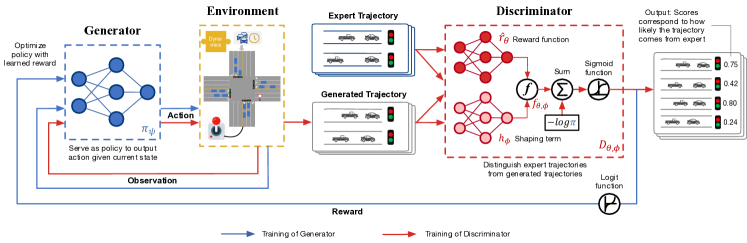
Figure 2: Overview of PS-AIRL. The discriminator and the generator are trained alternatively. When training the discriminator, the generator serves as a fixed policy that rollouts trajectories. The discriminator takes both generated and expert trajectories as input and distinguishes between them. When training the generator, the learned reward function is used as the cost function to update the optimal policy.

3 Problem Definition

We frame traffic simulation as a multi-agent control problem, regarding the complicated interaction between vehicles in traffic. Formally, we formulate our model in a decentralized partially observable Markov decision process (DPOMDP) defined by the tuple $(\mathcal{M},\{\mathcal{S}_{m}\},\{\mathcal{A}_{m}\},\mathcal{T},r,\gamma,\rho_{0})$. Here $\mathcal{M}$ denotes a finite set of agents, $\{\mathcal{S}_{m}\}$ and $\{\mathcal{A}_{m}\}$ the sets of states and actions for each agent $m$, respectively. We have $\mathcal{S}_{m}\in\mathbb{R}^{S}$ and $\mathcal{A}_{m}\in\mathbb{R}^{A}$ for all agents $m\in\mathcal{M}$. $\rho_{0}$ denotes the initial state distribution. $r(s,a)$ is the reward function, and $\gamma$ denotes the long-term reward discount factor. We assume for a set of given expert demonstrations, the environment dynamics remain unchanged. The deterministic state transition function is defined by $\mathcal{T}(s^{\prime}|s,a)$. We formulate the microscopic traffic simulation problem in a inverse reinforcement learning (IRL) fashion. Given trajectories of expert vehicles, our goal is to learn the reward function of the vehicle agent. Formally, the problem is defined as follows:

Problem 1

Given a set of expert trajectories as demonstrations $\mathcal{D}=\{\tau_{1},\tau_{2},...,\tau_{M}\}$ generated by an optimal policy $\pi^{*}(a|s)$ where $\tau=\{s_{1},a_{1},...,s_{T},a_{T}\}$, the goal is to recover the reward function $r_{\theta}(s,a)$, so that the log likelihood of the expert trajectories are maximized, i.e.,

$$\max_{\theta}E_{\tau\sim\mathcal{D}}[\log p_{\theta}(\tau)]$$ (1)

Here, $p_{\theta}(\tau)\propto\exp\{\sum_{t=0}^{T}\gamma^{t}r_{\theta}\left(s_{t},a_{t}\right)\}$ is the distribution of trajectories parameterized by $\theta$ in the reward $r_{\theta}(s,a)$.

4 Method

4.1 Adversarial Inverse Reinforcement Learning

Along the line of IRL,  Finn et al. (2016b) proposed to treat the optimization problem in Eq. (1) as a GAN-like Goodfellow et al. (2014) optimization problem. This adversarial training framework alternates between training the discriminator to classify each expert trajectory and updating the policy to adversarially confuse the discriminator, and optimize the loss:

$$\min_{\theta}\max_{\psi}{\mathbb{E}}_{\pi_{\psi}}\left[\log\left(D_{\theta}(s,a)\right)\right]+{\mathbb{E}}_{\pi_{E}}\left[\log\left(1-D_{\theta}(s,a)\right)\right]$$ (2)

where $D_{\theta}$ is the discriminator parameterized by $\theta$, $\pi_{E}$ is the optimal policy for expert demonstration data $\mathcal{D}$, and $\pi_{\psi}$ is the learned policy parameterized by $\psi$ in the generator. Specifically, the discriminator scores each sample with its likelihood of being from the expert, and use this score as the learning cost to train a policy that generates fake samples. Thus, the objective of the generator is to generate samples that confuse the discriminator, where $\log D_{\theta}(s,a)$ is used as a surrogate reward to help guide the generated policy into a region close to the expert policy. Its value grows larger as samples generated from $\pi_{\psi}$ look similar to those in expert data.

We use the same strategy to train a discriminator-generator network. However, one limitation of Finn et al. (2016b) is that, the use of full trajectories usually cause high variance. Instead, we follow Finn et al. (2016a) to use state-action pairs as input with a more straightforward conversion for the discriminator:

$$D(s,a)=\frac{\exp\{f(s,a)\}}{\exp\{f(s,a)\}+\pi(a|s)}$$ (3)

where $f$ is a learned function, and policy $\pi$ is trained to maximize reward $r(s,a)=\log(1-D(s,a))-\log D(s,a)$. In each iteration, the extracted reward serves as the learning cost for training the generator to update the policy. Updating the discriminator is equivalent to updating the reward function, and in turn updating the policy can be viewed as improving the sampling distribution used to estimate the discriminator. The structure of the discriminator in Eq. (3) can be viewed as a sigmoid function with input $f(s,a)-\log\pi$, as shown in Fig. 2. Similar to GAN, the discriminator is trained to reach the optimality when the expected $D(s,a)$ over all state-action pairs is $1/2$. At the optimality, $f^{*}(s,a)=\log\pi^{*}(a|s)$ and the reward can be extracted from the optimal discriminator by $r(s,a)=f(s,a)+Const$.

4.2 Dynamics-robust Reward Learning

We seek to learn the optimal policy for the vehicle agent from real-world demonstrations. So the learned policy should be close to, in the real world, the driver’s policy to control the movement of vehicles given the state of traffic environment. Despite the non-stationary nature of traffic dynamics, the vehicle’s objective during driving should constantly remain the same. This means that although the optimal policy under different system dynamics may vary, the vehicle constantly has the same reward function. Therefore, it is highly appealing to learn an underlying dynamic-robust reward function beneath the expert policy. By defining the traffic simulation learning as an IRL problem, we adapt the adversarial IRL (AIRL) as in Section 4.1 on the traffic simulation problem and propose a novel simulation model, which serves to not only imitate the expert trajectories (i.e., driving behaviors), but simultaneously recover the underlying reward function.

We aim to utilize the reward-invariant characteristics of AIRL to train an agent that simulates a vehicle’s behavior in traffic while being robust to dynamics with changing traffic environment. The reward ambiguity is an essential issue in IRL approaches. Ng et al. (1999) proposes a class of reward transformations that preserve the optimal policy, for any function $\Phi:\mathcal{S}\longrightarrow\mathbb{R}$, we have

$$\hat{r}(s,a,s^{\prime})\in\{\hat{r}|\hat{r}=r(s,a,s^{\prime})+\gamma\Phi(s^{\prime})-\Phi(s)\}$$ (4)

If the true reward is solely a function of state, we are able to extract a reward that is fully disentangled from dynamics (i.e., invariant to changing dynamics) and recover the ground truth reward up to a constant Fu et al. (2018).

To learn this dynamic-robust reward and ensure it remains in the set of rewards that correspond to the same optimal policy, AIRL follows the above reward transformation, and replaces the learned function $f(s,a)$ in Eq. (3) with

$$f_{\theta,\phi}(s,a,s^{\prime})=\hat{r}_{\theta}(s)+\gamma h_{\phi}(s^{\prime})-h_{\phi}(s)$$ (5)

where $\hat{r}_{\theta}(s)$ is the state-only reward approximator, $h_{\phi}$ is a shaping term, and $s^{\prime}=\pi(s,a)$ is the next state. The transformation in Eq. (5) ensures that the learned function $f_{\theta,\phi}$ corresponds to the same optimal policy as the reward approximator $\hat{r}_{\theta}$ does. Correspondingly, $D_{\theta}(s,a)$ in Eq. (3) becomes

$$D_{\theta,\phi}(s,a,s^{\prime})=\frac{\exp\{f_{\theta\phi}(s,a,s^{\prime})\}}{\exp\{f_{\theta\phi}(s,a,s^{\prime})\}+\pi(a|s)}$$ (6)

As a result, the discriminator can be represented by the combination of the two functions $\hat{r}_{\theta}$ and $h_{\phi}$ as shown in Fig. 2.

4.3 Parameter-sharing Agents

1

Input: Expert trajectories $\tau_{E}\sim\pi_{E}$

Output: Policy $\pi_{\psi}$, reward $r_{\theta,\phi}$

2

3Initialize policy parameters $\psi$, and discriminator parameters $\theta$ and $\phi$

4 for k $\longleftarrow$ 0, 1, … do

5       Rollout trajectories for all $M$ agents $\vec{\tau}=\{\tau_{1},\tau_{2},...,\tau_{M}\}\sim\pi_{\psi_{k}}$

6      

7      Update $\theta$, $\phi$ in discriminator given $\vec{\tau}$ via minimizing ${\mathbb{E}}_{\pi_{\psi}}\!\!\left[\log\left(D_{\theta,\phi}(s,a,s^{\prime})\right)\right]\!+\!{\mathbb{E}}_{\pi_{E}}\!\!\left[\log\left(1\!\!-\!\!D_{\theta,\phi}(s,a,s^{\prime})\right)\right]$

8      

9      Update reward using discriminator output $r_{\theta,\phi}\longleftarrow\log D_{\theta,\phi}-\log(1-D_{\theta,\phi})$

10      

11      Update policy $\pi_{\psi}$ with a TRPO step by solving the optimization in Eq. (7). Then $\pi_{\psi_{k+1}}\longleftarrow\pi_{\psi}$.

Algorithm 1 Training procedure of PS-AIRL

As illustrated in Section 3, we formulate the traffic simulation as multi-agent system problem by taking every vehicle in the traffic system as an agent interacting with the environment and each other. Inspired by parameter sharing trust region policy optimization (PS-TRPO) Gupta et al. (2017), we incorporate its decentralized parameter sharing training protocol with AIRL in Section 4.1, and propose the parameter sharing AIRL (PS-AIRL) that learns policies capable of simultaneously controlling multiple vehicles in complex traffic environment. In our formulation, the control is decentralized while the learning is not. Accordingly, we make some simple assumptions for the decentralized parameter sharing agents. See Appendix for details.

Under the decentralized parameter sharing training protocol as in Gupta et al. (2017), our proposed PS-AIRL can be highly sample-efficient since it reduces the number of parameters by a factor $M$, and shares experience across all agents in the environment. We use TRPO Schulman et al. (2015) as our policy optimizer, which allows precise control of the expected policy improvement during the optimization. For a policy $\pi_{\psi}$, at each iteration $k$, we perform an update to the policy parameters $\psi$ by solving the following problem:

$$\begin{split}\min_{\psi}\ \ \mathbb{E}_{s,a\sim\pi_{\psi_{k}},m\in\mathcal{M}}&\left[\frac{\pi_{\psi}(a|s,m)}{\pi_{\psi_{k}}(a|s,m)}A_{\psi_{k}}(s,m,a)\right]\\ s.t.,\ \ \mathbb{E}_{s\sim\pi_{\psi_{k}}}&\left[D_{\mathrm{KL}}\left(\pi_{\psi_{k}}\|\pi_{\psi}\right)\right]\leq\delta\end{split}$$ (7)

where $\pi_{\psi_{k}}$ is the policy obtained in the previous iteration, $A_{\psi_{k}}(s,m,a)$ is an advantage function that can be estimated by the difference between the empirically predicted value of action and the baseline value. The training procedure of PS-AIRL is shown in Algorithm 1. The training pipeline details can be found in the appendix.

5 Experiment

Method	HZ-1		HZ-2		HZ-3		GD		LA
	Pos	Speed	Pos	Speed	Pos	Speed	Pos	Speed	Pos	Speed
CFM-RS	173.0	5.3	153.0	5.6	129.0	5.7	286.0	5.3	1280.9	10.3
CFM-TS	188.3	5.8	147.0	6.1	149.0	6.1	310.0	5.5	1294.7	10.8
PS-AIRL	120.9	4.5	41.0	2.1	10.7	1.1	45.6	1.0	681.5	5.1
Improvement	30.1%	15.1%	72.1%	47.6%	91.7%	80.7%	84.1%	81.1%	46.8%	50.5%

Table 1: Performance comparison of PS-AIRL with state-of-art methods in terms of RMSE of recovered vehicle position (m) and speed (m/s).

We generally aim to answer the following three questions.

• Q1: Trajectory simulation. Is PS-AIRL better at imitating the vehicle movement in expert trajectories?

• Q2: Reward recovery. Can PS-AIRL learn the vehicle’s objective by recovering the reward function?

• Q3: Capability to generalize. Is the recovered reward function robust to dynamics changes in the traffic environment?

5.1 Data and Experiment Setting

We evaluate our proposed model on 3 different real-world traffic trajectory datasets with distinct road network structures collected from Hangzhou of China, and Los Angeles of US, including 3 typical 4-way intersections, a $4\times 4$ network, and a $1\times 4$ arterial network. See Appendix for details.

We compared PS-AIRL to two traditional CFM-based methods, CFM-RS and CRF-TS Krauß (1998), and three imitation learning-based models, BC Michie et al. (1990), DeepIRL Wulfmeier et al. (2015) and MA-GAIL Zheng et al. (2020). See Appendix for details.

We use root mean square error (RMSE) to evaluate the mismatch between ground truth traffic trajectories and the trajectories generated by the simulation model. In addition, to verify the capacity of PS-AIRL in recovering the underlying reward that can generalize to different dynamics, we compare the reward values each model reaches given a hand-crafted reward function. See Appendix for its definition.

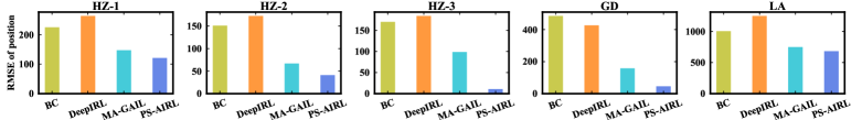
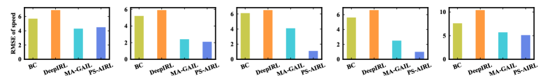
Figure 3: Performance comparison of variants of learning methods in terms of RMSE of position. PS-AIRL beats all alternatives.

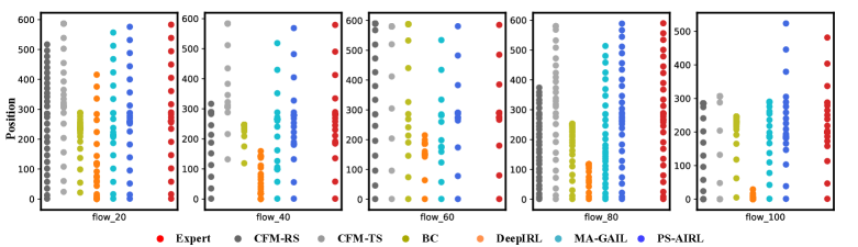
Figure 4: Trajectories of vehicles recovered by different methods on HZ-3. We arbitrarily select the vehicles with id 20, 40, 60, 80 and 100 and show their position w.r.t time. The position of vehicles recovered by PS-AIRL (blue) is most similar to the Expert (red).

5.2 Traffic Simulation

To answer Q1, we evaluate each model by using them to recover traffic trajectories, as shown in Table 1 and Figure 3.

We first compare our proposed algorithm with state-of-art simulation algorithms CFM-RS and CFM-TS (as in Table 1). We can observe that our proposed PS-AIRL outperforms the baseline methods on all datasets. The two traditional methods CFM-RS and CFM-TS perform poorly due to the generally inferior fitting ability of physical CFM models against sophisticated traffic environment. We further compare PS-AIRL with state-of-art imitation learning methods. The results are shown in Figure 3. We can observe that PS-AIRL performs consistently better than other baselines. Specifically, as expected, PS-AIRL and MA-GAIL perform better than the other two, for they can not only model the sequential decision process (compared to BC) and utilize the adversarial process to improve the imitation (compared to DeepIRL). More importantly, PS-AIRL achieves superior performance over MA-GAIL (except in HZ-1 these two perform similarly in terms of RMSE of speed). It indicates that our proposed model benefits from the learned invariant reward. For instance, if one vehicle enter the system right after another, we may not expect it to accelerate a lot. In contrast, if one vehicle enter the system with no preceding vehicle, it may speed up freely within the speed limit. Behaviors may seem different under these two cases, but the reward function still remains the same. Therefore, armed with explicit reward learning, PS-AIRL is able to outperform.

Simulation Case Study To have a closer look at the simulation of vehicle behavior, we extract the learned trajectory of 5 vehicles (vehicles with id 20, 40, 60, 80, 100) from HZ-3 as examples. Comparison between trajectories generated by different methods is shown in Fig. 4. The trajectories recovered by PS-AIRL are most similar to the expert ones.

5.3 Objective Recovery

To answer Q2, we leverage a hand-designed reward function as the ground truth and let the algorithms recover it. The reward increases when the vehicle approaches its desired speed and succeed in keeping safe distance from its preceding vehicles (see Appendix for details). Specifically, we use this hand-designed reward function to train an expert policy and use the generated expert trajectories to train each method. Note that, CFM-based methods are not included here for the following reasons. CFM-based methods can yield very unreal parameters (e.g., acceleration of 10 $m/s^{2}$) to match the generated trajectory. These will cause collision of vehicles or even one vehicle directly pass through another. This is an unreal setting. Hence, these CFM-based methods can not recover the true policy that vehicles follow in the simulation.

Achieved Reward Value We conduct experiments on HZ-1, HZ-2, HZ-3 and GD, and the results are shown in Table 2. As expected, PS-AIRL achieves higher reward than other baselines and approach much closer to the upper bound reward value provided by the Expert. This indicates the better imitation (i.e. simulation) power of PS-AIRL.

Method	HZ-1	HZ-2	HZ-3	GD
BC	-0.345	-0.277	-0.248	-0.349
DeepIRL	-0.586	-0.238	-0.311	-0.360
MA-GAIL	-0.524	-0.210	-0.228	-0.181
PS-AIRL	-0.173	-0.203	-0.201	-0.161
Expert	-0.060	-0.052	-0.062	-0.065

Table 2: Achieved reward of different imitation learning methods. Higher reward indicates better imitation of the expert.

Recovered Reward Function We are also interested in whether PS-AIRL can recover the groundtruth reward function. Hence, we visualize the reward function learned by PS-AIRL and the surrogate reward of MA-GAIL (the best baseline). Due to the space limit, results from other methods are omitted. They generally show even worse results than MA-GAIL. We enumerate the reward values for different speed and gap values. (Other state feature values are set to default values.) As in Fig. 5, compared to MA-GAIL, PS-AIRL recovers a reward closer to the groundtruth yet with a smoother shape. Our designed reward function applies penalties on slow speed and unsafe small gap. So the expert policy trained with this groundtruth reward tends to drive the vehicle on a faster speed and keep it against the front vehicle out of the safety gap. It shows that PS-AIRL is able to learn this objective of the expert in choosing optimal policies from demonstrations, assigning higher reward values to states with faster speed and safe gap, while applying penalties on the opposite. In contrast, the surrogate reward learned by the MA-GAIL totally ignores the safe gap. In addition, when vehicles are out of the safe gap, PS-AIRL recovered a reward value closer to the groudtruth.

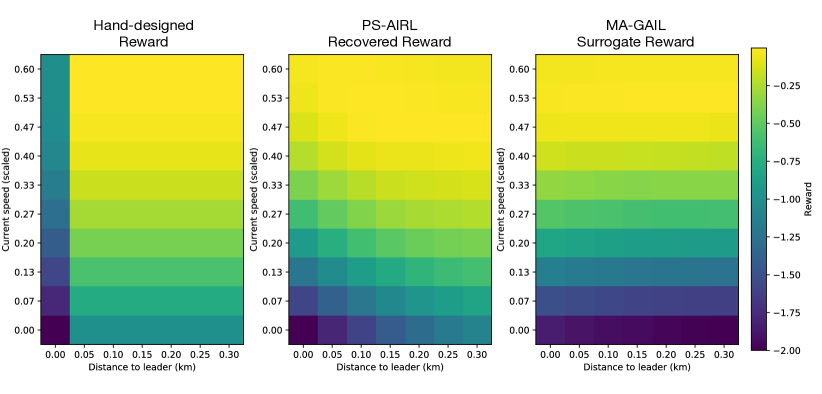
Figure 5: Hand-designed reward (groundtruth), recovered reward of PS-AIRL and surrogate reward (output of discriminator) of MA-GAIL w.r.t. current speed and gap, on HZ-1. PS-AIRL can better infer the groundtruth reward function.

5.4 Robustness to Dynamics

To answer Q3, we transfer the model learned in Section 5.3 to a new system dynamics. Specifically, compared with Section 5.3, we change the maximum acceleration and deceleration of vehicles from initially 2 $m/s^{2}$ and 4 $m/s^{2}$ into 5 $m/s^{2}$ and 5 $m/s^{2}$ respectively. Other settings remain unchanged. Because the reward function remains unchanged (i.e., drivers still want to drive as fast as possible but keep a safe gap), reward-learning methods should be able to generalize well.

For DeepIRL, MA-GAIL and PS-AIRL, we use the learned reward function (surrogate reward function for MA-GAIL) to train a new policy. (BC policy is directly transferred because it do not learn reward function.) We also include a direct transfer version of PS-AIRL as comparison to demonstrate the necessity of re-training policy under new dynamics. Similar to the reward recovery experiment, CFM models also do not apply to this comparison.

Method	HZ-1	HZ-2	HZ-3	GD
BC ($\mathcal{D}$)	-0.406	-0.322	-0.336	-0.681
DeepIRL	-0.586	-0.288	-0.362	-0.369
MA-GAIL	-0.483	-0.243	-0.337	-0.175
PS-AIRL ($\mathcal{D}$)	-0.448	-0.254	-0.321	-0.598
PS-AIRL	-0.384	-0.192	-0.248	-0.161

Table 3: Reward under new dynamics. BC ($\mathcal{D}$) and PS-AIRL ($\mathcal{D}$) means directly applying the learned policy. The other methods use the learned reward to retrain a policy under new dynamics.

Table 3 shows the achieved reward in the new environment. PS-AIRL achieves highest reward, because with the invariant reward function learned from the training environment, PS-AIRL can learn a new policy that adapts to the changed environment. DeepIRL perform poorly in transferred environment because of its incapability of dealing with large number of states. PS-AIRL ($\mathcal{D}$) fails to generalize to the new environment, which indicates that the policy learned in the old dynamics are not applicable anymore. MA-GAIL, though retrained with the surrogate reward function, can not transfer well, due to the dependency on the system dynamics.

6 Conclusion

In this paper, we formulated the traffic simulation problem as a multi-agent inverse reinforcement learning problem, and proposed PS-AIRL that directly learns the policy and reward function from demonstrations. Different from traditional methods, PS-AIRL does not need any prior knowledge in advance. It infers the vehicle’s true objective and a new policy under new traffic dynamics, which enables us to build a dynamics-robust traffic simulation framework with PS-AIRL. Extensive experiments on both synthetic and real-world datasets show the superior performances of PS-AIRL on imitation learning tasks over the baselines and its better generalization ability to variant system dynamics.

Appendix A Simulation Environment

We created an OpenAI Gym environment as our simulation environment based on the a traffic simulator called CityFlow Zhang et al. (2019). CityFlow is an efficient traditional car-following model (CFM) based traffic simulator that is able to conduct 72 steps of simulations per second for thousands of vehicles on large scale road networks using 8 threads. The CFM used in CityFlow is a modification of the Krauss car-following model with the key idea that, the vehicle will drive as fast as possible subject to perfect safety regularization. The vehicles in CityFlow are subject to several speed constraints, and will drive in the maximum speed that simultaneously meets all these constraints.

This CityFlow-based environment is able to provide multiple control APIs that allow us to obtain observations and give vehicles direct controls that bypasses the embedded default CFM. At each timestep, for a certain vehicle, a state representation is generated from the environment. The policy will determine the best action (i.e., next step speed) according to the state and conduct it on the environment. Since we do not have trajectory data in granularity of seconds, on the HZ and GD roadnets in our experiments (Section VI), we use CityFlow to generate trajectories as demonstration data based on real traffic flow. In these demonstration datasets, the embedded CFM in CityFlow serves as an expert policy. But during simulation learning, the embedded CFM has no effect on the learned policy. For the LA dataset, we directly extract the vehicle trajectories from the dataset.

This environment is initiated with a road network, traffic flow, and a signal plan. The road network includes information of intersections, roads, and length of each lane. The traffic flow provides the track of each vehicle, as well as the time and location it enters the system. The traffic signal plan gives the phase of traffic light for each intersection.

Appendix B Dataset

Hangzhou (HZ). This dataset covers three typical 4-way intersections in Hangzhou, China, collected from surveillance cameras near intersections in 2016. Each record contains the vehicle id, arriving time and location. Based on this, we use the default simulation environment of CityFlow Zhang et al. (2019) (in Section 5.2) or trained by a hand-designed reward function (in Section 5.3 and 5.4) to generate expert demonstration trajectories, denoted to as HZ-1, HZ-2, and HZ-3.

Gudang (GD). This a $4\times 4$ network of Gudang area (Figure 6 (a)) in Hangzhou, collected in same fashion as HZ dataset. This region has relatively dense surveillance cameras. Necessary missing data fill in are conducted. We process it in the same way as HZ dataset.

Los Angeles (LA). This is a public traffic dataset  collected from Lankershim Boulevard, Los Angeles on June 16, 2005. It covers an $1\times 4$ arterial with four successive intersections (shown in Figure 6 (b)). This dataset records the position and speed of every vehicle at every 0.1 second. We directly use these records as expert trajectories.

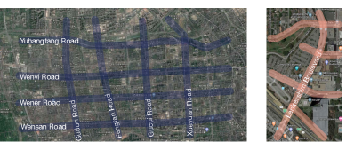
(a) Gudang, Hangzhou

(b) LA

Figure 6: Maps of the $4\times 4$ roadnet of Gudang Area, Hangzhou and the $1\times 4$ roadnet of Lankershim Boulevard, LA used in our experiment.

Appendix C Compaired Baselines

Traditional CRF-based Method

• CFM-RS: the CFM calibrated with random search. In each trial, a set of parameters for the Krauss model is randomly selected given a limited searching parameter space. After limited times of trials, the set of parameters that yields trajectories most similar to demonstrations is kept as the calibration result.

• CFM-TS: the CFM calibrated with Tabu search Osorio and Punzo (2019). Given an initial set of parameters, a new set is chosen within the neighbors of the current parameter set. The new set of parameters will be included in the Tabu list, if they generates better trajectories. The best set of parameters in the Tabu list is shown in the results.

Imitation Learning Method

• BC: behavioral cloning Michie et al. (1990) is a typical imitation learning method with a supervised learning procedure. It directly trains a policy network to fit the state-action mapping.

• DeepIRL: maximum entropy deep IRL Wulfmeier et al. (2015). Since it is unable to deal with large state space, in our experiments, we use spectral clustering Ng et al. (2002) to discretize the state extracted from the environment into 64 states as the input of DeepIRL.

• MA-GAIL: An extension of GAIL Zheng et al. (2020) for traffic simulation.

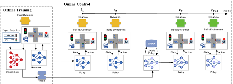
Figure 7: The dynamics-robust framework of our PS-AIRL simulation model. The policy and reward are both learned during the offline training. During online control of the simulator, the learned policy plays the role of controlling the movement of vehicles in the environment. We employ TRPO to regularly optimize a new policy with the learned reward function. No expert demonstrations are needed for policy re-optimization.

Appendix D Evaluation Metrics

We evaluate the trajectories generated by the policies of each method against the expert trajectories, using root mean square error (RMSE) of position and speed. The RMSE of position is defined as $RMSE=\frac{1}{T}\sum_{t=1}^{T}\sqrt{\frac{1}{m}\sum_{j=1}^{m}\left(s_{j}^{(t)}-\hat{s}_{j}^{(t)}\right)^{2}}$, where $T$ is total time of the simulation, $s_{j}^{(t)}$ and $\hat{s}_{j}^{(t)}$ are the true value and observed value of the position of the $j$-th vehicle at timestep $t$, respectively. The RMSE of speed is calculated similarly.

D.0.1 Hand-crafted Reward

In order to verify the capability of PS-AIRL to recover reward function and generalize to different dynamics, we further compare the reward values that different methods can reach. We use the hand-crafted reward function defined in Eq. 8 as the ground truth reward. For each vehicle at each timestep, we define its reward $r$ as the opposite of the match error of its speed $v$ and gap $g$ (distance to the preceding vehicle or the traffic light) against the desired speed $v_{des}$ and gap $g_{des}$.

$$r=-\left[\left(\frac{v-v_{des}}{v_{max}}\right)^{2}+\lambda\left(\frac{g-g_{des}}{g_{min}}\right)^{2}\right]$$ (8)

where $\lambda$ is a trade-off parameter, $v_{max}$ and $g_{min}$ are the speed limit in the current lane and the given minimum gap between vehicles. The $v_{des}$ and $g_{des}$ are determined according to the traffic signal status, speed limit and distance to the leading vehicle. In Section 5.3 and 5.4, we use the mean reward value $\bar{r}$ (first averaged by a vehicle’s episode length, and then averaged by the total number of vehicles in system) as the evaluation metric.

For the hand-crafted reward, we determine the desired speed and the desired gap as in Figure 8. Basically, the vehicle desires to keep a speed as high as the max speed when possible, and to decelerate to a safe speed if it is too close to a preceding vehicle or a red traffic signal. In addition, the the vehicle aims to maintain a gap from the preceding vehicle larger or equal to the minimum gap. In Section 5.3, we set $\lambda\!=\!1$, $v_{max}=11m/s$ and $g_{min}=25m$.

Feature Type	Detail Features
Road network	Lane ID, Length of current Lane, Speed limit
Traffic signal	Phase of traffic light
Vehicle	Velocity, Position in lane, Distance to traffic light
Preceding vehicle	Velocity, Position in lane, Gap to preceding vehicle
Indicators	If leading in current lane, If exit from intersection

Table 4: Observation features.

Appendix E Reward and System Dynamics

Similar to human driver’s decision making, reward function and system dynamics are the two key components that determines a vehicle’s driving policy (as illustrated in Figure 9). The reward function can be view as how the a vehicle values different state components during driving, e.g., safety and efficiency. For instance, a real-world vehicle usually attempts to drive as fast as it can under the assumption that it is safe (e.g., keeping a safe distance to the preceding vehicle). A driving policy is formed by selecting actions that maximize their expected reward. System dynamics, on the other hand, describes how the vehicle’s actions yield the next state of environment. System dynamics consist of some physical factors including road conditions (e.g., speed limit, road surface and weather condition) and vehicle properties (e.g., maximum speed, maximum acceleration and maximum deceleration). The difference of these factors in different time and locations may lead to the change of system dynamics.

Appendix F Assumptions

In our formulation, the control is decentralized while the learning is not Gupta et al. (2017). Accordingly, we make simple assumptions for our decentralized parameter sharing agents as follows.

• Agent: Each vehicle as an independent agent $m\in\mathcal{M}$, cannot explicitly communicate with each other but can learn cooperative behaviors only from observations.

• State and Action: We select a set of features to define observations (partially observed state), as shown in Table 4 in Appendix. We use speed as action for each vehicle agent. In each timestep the agent makes a decision in choosing a speed for the next timestep. Each agent has the same state and action space:

  $$\mathcal{S}_{m}\in\mathbb{R}^{S}\ \text{and}\ \mathcal{A}_{m}\in\mathbb{R}^{A},\forall m\in\mathcal{M}$$

• Policy: All agents share the parameters of a homogeneous policy $\pi(a|s)$. This enables the policy to be trained with the experiences of all agents at the same time, while it still allows different actions between agents since each agent has independent different observations.

• Reward: All agents share the parameters of a homogeneous unknown reward function $r(s,a)$. Accordingly, each vehicle agent gets distinct reward given different observations and actions.

Appendix G Network Architectures

Our whole model can be divided into two parts, discriminator and generator. The network structure and size are shown in Table 5.

Discriminator. In our PS-AIRL, the discriminator is composed of two networks, the reward function $\hat{r}_{\theta}$ and the shaping term $h_{\phi}$, as well as a sigmoid function. Concretely, the reward function $\hat{r}_{\theta}$ only takes state as input and output the estimation of the disentangled reward for the current state. The shaping term $h_{\phi}$ also takes state features as input, as a regularization to the reward $\hat{r}_{\theta}$ that helps mitigate the reward ambiguity effect. The whole network of the discriminator $D_{\theta,\phi}$ can be presented as follows

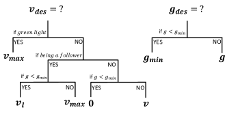
Figure 8: Calculation of desired speed $v_{des}$ and desired gap $g_{des}$ in the hand-designed reward function, where $v$ and $v_{l}$ are the velocity of the focused vehicle and its preceding vehicle, $v_{max}$ and $g_{min}$ is the given speed limit and desired minimum gap, and $g$ is the gap against the front car.

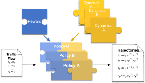
Figure 9: Reward, system dynamics and policy. Ideally, the reward with distinct system dynamics remains the same.

$$\begin{split}\hat{r}_{\theta}(s)&=\text{ReLU-Net}_{\theta}(s)\\ h_{\phi}(s)&=\text{ReLU-Net}_{\phi}(s)\\ f_{\theta,\phi}(s,a,s^{\prime})&=\hat{r}_{\theta}(s)+\gamma h_{\phi}(s^{\prime})-h_{\phi}(s)\\ D_{\theta,\phi}(s,a,s^{\prime})&=\sigma\left(f_{\theta,\phi}(s,a,s^{\prime})-\log\pi(a|s)\right)\end{split}$$ (9)

where $s$ is the current state, $s^{\prime}$ is the state for the next timestep, $\text{ReLU-Net}(\cdot)$ is a ReLU network with two hidden layers, $\sigma(\cdot)$ is a sigmoid function, and $\pi$ is the learned policy during the last iteration.

Generator (policy). The generator is using an actor-critic agent optimized by trust region policy optimization (TRPO). In detail, we use Beta distribution in the actor network, as it can restrict the range of the output action. The actor network takes state as input, and outputs the values of two parameters for the distribution. Then we sample action from the distribution determined by these two parameters. For the critic network, it takes the state features as input and outputs the estimation of the value of current state.

Some of the key hyperparameters are shown in Table 6.

Table 5: Summary of network structures. FC stands for fully-connected layers. Here, ($11+M$,) is the dimension for the state features, where $M$ is the number of lanes in the environment. This is because we use one-hot encoding for the lane id feature.

Network	$\hat{r}_{\theta}$	$h_{\phi}$	Actor	Critic
Input	($11+M$,)	($11+M$,)	($11+M$,)	($11+M$,)
Hidden layers	FC(32)	FC(32)	FC(32)	FC(32)
	FC(32)	FC(32)	FC(32)	FC(32)
Activation	ReLU	ReLU	ReLU	ReLU
Output	(1,)	(1,)	(2,)	(1,)

Table 6: Summary of hyperparameters

Hyperparameters	Value
Update period (timestep)	50
Discriminator update epoch	5
Generator (policy) update epoch	10
Batch size	64
Learning rate $\alpha$	0.001

Appendix H Details of Training Pipeline

Fig. 7 shows an overview of our dynamics-robust traffic simulation framework. Given a set of initial expert demonstrations, PS-AIRL learns an optimal policy and the reward function. During simulation, the learned policy plays the role of controlling the vehicles’ behaviors. In the meantime, a TRPO step is applied to optimize the policy regularly every once in a while, so that the continuously updated policy can better fit the naturally non-stationary traffic environment. During this process, no expert demonstrations are needed any more.

References

- Barceló and Casas (2005) Jaime Barceló and Jordi Casas. Dynamic network simulation with aimsun. In Simulation approaches in transportation analysis, pages 57–98. Springer, 2005.
- Bhattacharyya et al. (2018) Raunak P Bhattacharyya, Derek J Phillips, Blake Wulfe, Jeremy Morton, Alex Kuefler, and Mykel J Kochenderfer. Multi-agent imitation learning for driving simulation. In 2018 IEEE/RSJ International Conference on Intelligent Robots and Systems (IROS), pages 1534–1539. IEEE, 2018.
- Finn et al. (2016a) Chelsea Finn, Paul Christiano, Pieter Abbeel, and Sergey Levine. A connection between generative adversarial networks, inverse reinforcement learning, and energy-based models. In Advances in Neural Information Processing Systems (NeurIPS), 2016.
- Finn et al. (2016b) Chelsea Finn, Sergey Levine, and Pieter Abbeel. Guided cost learning: Deep inverse optimal control via policy optimization. In International Conference on Machine Learning (ICML), pages 49–58, 2016.
- Fu et al. (2018) Justin Fu, Katie Luo, and Sergey Levine. Learning robust rewards with adversarial inverse reinforcement learning. International Conference on Learning Representations (ICLR), 2018.
- Goodfellow et al. (2014) Ian Goodfellow, Jean Pouget-Abadie, Mehdi Mirza, Bing Xu, David Warde-Farley, Sherjil Ozair, Aaron Courville, and Yoshua Bengio. Generative adversarial nets. In Advances in Neural Information Processing Systems (NeurIPS), pages 2672–2680, 2014.
- Gupta et al. (2017) Jayesh K Gupta, Maxim Egorov, and Mykel Kochenderfer. Cooperative multi-agent control using deep reinforcement learning. In International Conference on Autonomous Agents and Multiagent Systems, pages 66–83. Springer, 2017.
- Ho and Ermon (2016) Jonathan Ho and Stefano Ermon. Generative adversarial imitation learning. In Advances in Neural Information Processing Systems (NeurIPS), pages 4565–4573, 2016.
- Krajzewicz et al. (2012) Daniel Krajzewicz, Jakob Erdmann, Michael Behrisch, and Laura Bieker. Recent development and applications of SUMO - Simulation of Urban MObility. International Journal On Advances in Systems and Measurements, 5(3&4):128–138, December 2012.
- Krauß (1998) Stefan Krauß. Microscopic modeling of traffic flow: Investigation of collision free vehicle dynamics. PhD thesis, Dt. Zentrum für Luft-und Raumfahrt eV, Abt., 1998.
- Michie et al. (1990) D Michie, M Bain, and J Hayes-Miches. Cognitive models from subcognitive skills. IEEE control engineering series, 44:71–99, 1990.
- Ng et al. (1999) Andrew Y Ng, Daishi Harada, and Stuart Russell. Policy invariance under reward transformations: Theory and application to reward shaping. In ICML, volume 99, pages 278–287, 1999.
- Ng et al. (2002) Andrew Y Ng, Michael I Jordan, Yair Weiss, et al. On spectral clustering: Analysis and an algorithm. In Advances in Neural Information Processing Systems (NeurIPS), volume 2, pages 849–856, 2002.
- Osorio and Punzo (2019) Carolina Osorio and Vincenzo Punzo. Efficient calibration of microscopic car-following models for large-scale stochastic network simulators. Transportation Research Part B: Methodological, 119:156–173, 2019.
- Schulman et al. (2015) John Schulman, Sergey Levine, Philipp Moritz, Michael I Jordan, and Pieter Abbeel. Trust region policy optimization. In Proceedings of the International Conference on Machine learning (ICML), 2015.
- Toledo et al. (2003) Tomer Toledo, Haris N Koutsopoulos, Angus Davol, Moshe E Ben-Akiva, Wilco Burghout, Ingmar Andréasson, Tobias Johansson, and Christen Lundin. Calibration and validation of microscopic traffic simulation tools: Stockholm case study. Transportation Research Record, 1831(1):65–75, 2003.
- Wang et al. (2018) Sen Wang, Daoyuan Jia, and Xinshuo Weng. Deep reinforcement learning for autonomous driving. IEEE Transactions on Intelligent Transportation Systems, 2018.
- Wei et al. (2018) Hua Wei, Guanjie Zheng, Huaxiu Yao, and Zhenhui Li. Intellilight: A reinforcement learning approach for intelligent traffic light control. In Proceedings of the 24th ACM SIGKDD International Conference on Knowledge Discovery & Data Mining, pages 2496–2505. ACM, 2018.
- Wulfmeier et al. (2015) Markus Wulfmeier, Peter Ondruska, and Ingmar Posner. Maximum entropy deep inverse reinforcement learning. arXiv preprint arXiv:1507.04888, 2015.
- Yang and Koutsopoulos (1996) Qi Yang and Haris N Koutsopoulos. A microscopic traffic simulator for evaluation of dynamic traffic management systems. Transportation Research Part C: Emerging Technologies, 4(3):113–129, 1996.
- Yu and Fan (2017) Miao Yu and Wei David Fan. Calibration of microscopic traffic simulation models using metaheuristic algorithms. International Journal of Transportation Science and Technology, 6(1):63–77, 2017.
- Zhang et al. (2019) Huichu Zhang, Siyuan Feng, Chang Liu, Yaoyao Ding, Yichen Zhu, Zihan Zhou, Weinan Zhang, Yong Yu, Haiming Jin, and Zhenhui Li. Cityflow: A multi-agent reinforcement learning environment for large scale city traffic scenario. In International World Wide Web Conference (WWW) Demo Paper, 2019.
- Zheng et al. (2020) G. Zheng, H. Liu, K. Xu, and Z. Li. Learning to simulate vehicle trajectories from demonstrations. In ICDE, pages 1822–1825, 2020.