Uncertainty quantification through Monte Carlo method in a cloud computing setting

Abstract

The Monte Carlo (MC) method is the most common technique used for uncertainty quantification, due to its simplicity and good statistical results. However, its computational cost is extremely high, and, in many cases, prohibitive. Fortunately, the MC algorithm is easily parallelizable, which allows its use in simulations where the computation of a single realization is very costly. This work presents a methodology for the parallelization of the MC method, in the context of cloud computing. This strategy is based on the MapReduce paradigm, and allows an efficient distribution of tasks in the cloud. This methodology is illustrated on a problem of structural dynamics that is subject to uncertainties. The results show that the technique is capable of producing good results concerning statistical moments of low order. It is shown that even a simple problem may require many realizations for convergence of histograms, which makes the cloud computing strategy very attractive (due to its high scalability capacity and low-cost). Additionally, the results regarding the time of processing and storage space usage allow one to qualify this new methodology as a solution for simulations that require a number of MC realizations beyond the standard.

1 Introduction

Most of the predictions that are necessary for decision making in engineering, economics, actuarial sciences, and so on., are made based on computer models. These models are based on assumptions that may or may not be in accordance with reality. Thus, a model can have uncertainties on its predictions, due to possible wrong assumptions made during its conception. This source of variability on the response of a model is called model uncertainty [1]. In addition to modeling errors, the response of a model is also subject to variabilities due to uncertainties on model parameters, which may be due to measurement errors, imperfections in the manufacturing process, and other factors. This second source of randomness on the models response is called data uncertainty [1].

One way to take into account these uncertainties is to use the theory of probability, to describe the uncertain parameters as random variables, random processes, and/or random fields. This approach allows one to obtain a model where it is possible to quantify the variability of the response. For instance, the reader can see from [2, 3] where techniques of stochastic modeling are applied to describe the dynamics of a drillstring. Other applications in structural dynamics can be seen in [4, 5]. It is also worth mentioning the contributions of [6], in the context of hydraulic fracturing, [7], for estimation of financial reserves, and in [8] for the analysis of structures built by heterogeneous hyperelastic materials. For a deeper insight into stochastic modeling, with an emphasis in structural dynamics, the reader is encouraged to read [1, 9, 10].

To compute the propagation of uncertainties of the random parameters through the model, the most used technique in the literature is the Monte Carlo (MC) method [11]. This technique generates several realizations (samples) of the random parameters according to their distributions (stochastic model). Each of these realizations defines a deterministic problem, which is solved (processing) using a deterministic technique, generating an amount of data. Then, all of these data are combined through statistics to access the response of the random system under analysis [12, 13, 14]. A general overview of the MC algorithm can be seen in the Figure 1.

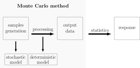
Figure 1: General overview of Monte Carlo algorithm.

The MC method does not require that one implements a new computer code to simulate a stochastic model. If a deterministic code to simulate a similar deterministic model is available, the stochastic simulation can be performed by running the deterministic program several times, changing only the parameters that are randomly generated. This nonintrusive characteristic is a great advantage of MC when compared with other methods for uncertainty quantification, such as generalized Polynomial Chaos (gPC), [15], which demands a new code for each new random system that one wants to simulate. Additionally, if the MC simulation is performed for a large number of samples, it completely describes the statistical behavior of the random system. Unfortunately, MC is a very time-consuming method, which makes unfeasible its use for complex simulations, when the processing time of a single realization is very large or the number of realizations to an accurate result is huge [12, 13, 14].

Meanwhile, the MC method algorithm can easily be parallelized because each realization can be done separately and then aggregated to calculate the statistics. The parallelization of the MC algorithm allows one to obtain significant gains in terms of processing time, which can enable the use of the MC method in complex simulations. In this context, cloud computing can be a very fruitful tool to enable the use of the MC method to access complex stochastic models because it is a natural environment for implementation of parallelization strategies. Moreover, in theory, cloud computing offers almost infinite scalability in terms of storage space, memory and processing capability, with a financial cost significantly lower than the one that is necessary to acquire a traditional cluster with the same capacity.

In this spirit, this work presents a methodology for implementing the MC method in a cloud computing setting, which is inspired by the MapReduce paradigm [16]. This approach consists of splitting, among several instances of the cloud environment, the MC calculation, processing each one of these tasks in parallel, and finally merging the results into a single instance to compute the statistics. As an example, the methodology is applied to a simple problem of stochastic structural dynamics. The use of cloud in not new in the context of engineering and sciences [17]. We would like to mention the work of Ari and Muhtaroglu [18] that proposes a cloud computing service for finite element analysis, the work of Jorissen et al. [19] that proposes a scientific cloud computing platform that offers high performance computation capability for materials simulations, and the work of Wang et al. [20] that discusses the Cumulus cloud based project with its applications to scientific computing, just to cite a few.

This paper is organized as follows. Section 2 makes a brief presentation of the cloud computing concept. Section 3 presents a parallelization strategy for the MC method in the context of cloud computing. Section 4 describes the case of study in which the proposed methodology is exemplified. Section 5 presents and discusses the statistics done with the data and the convergence of the results. Finally, section 6 presents the conclusions and highlights the main contribution of this work.

2 Cloud computing

Traditionally, the term cloud is a metaphor about the way the Internet is usually represented in network diagrams. In these diagrams, the icon of the cloud represents all the technologies that make the Internet work, ignoring the infrastructure and complexity that it includes. Likewise, the term cloud has been used as an abstraction for a combination of various computer technologies and paradigms, e.g., virtualization, utility computing, grid computing, service-oriented architecture and others, which together provide computational resources on demand, such as storage, database, bandwidth and processing [21].

Therefore, cloud computing can be understood as a style of computing where information technology capabilities are elastic, scalable, and are provided as services to the users via the Internet [22, 23]. In this style of computing, the computational resources are provided for the users on demand, as a pay-as-you-go business model, where they only need to pay for the resources that were effectively used. Due to its great potential for solving practical problems of computing, it is recognized as one of the top five emerging technologies that will have a major impact on the quality of science and society over the next 20 years [24].

The reader can see from [25] a detailed comparison between three cloud providers (Amazon EC2, Microsoft Azure and Rackspace) and a traditional cluster of machines. These experiments were done using the well-known NAS parallel benchmarks as an example of general scientific application. That article demonstrates that the cloud can have a higher performance and cost efficiency than a traditional cluster.

Furthermore, a traditional cluster require huge investments in hardware and in their maintenance and one can not “turn off resources contracts”, while they are unnecessary, to save money. Then, traditional clusters are almost prohibitive for scientific research without large financial resources.

In a cloud computing environment one pays only per hour of use of one virtual machine. Other costs of this platform are the shared/redundant storage and data transfers. For the data transfer, all inbound data transfers (i.e., data going to the cloud) are free and the price for outbound data transfers (i.e., data going out of the cloud) is a small cost that depends on the volume of data transferred.

Given these characteristics, it is easy to imagine a situation where computational resources can be turned on and off according to demand, providing unprecedented savings compared with acquisition and maintenance of a traditional cluster. In addition, if it is possible to parallelize the execution, the total duration of the process can be minimized using more virtual machines of the cloud.

3 Parallelization of Monte Carlo method in the cloud

The strategy to run the MC algorithm in parallel, as proposed in this work is influenced by the MapReduce paradigm [16], which was originally presented to support the processing of large collections of data in parallel and distributed environments. This paradigm consists in two phases: the first (Map) divides the computational job into several partitions and each partition is executed in parallel by different machines; the second phase (Reduce) collects the partial results returned by each machine, aggregates partial results and computes a response to the computational job.

We propose a MapReduce strategy for parallel execution in the cloud of the MC method that is composed of three steps: split, process, and merge. The split and the process steps correspond to the Map, while the merge corresponds to the Reduce step. This strategy of parallelization was implemented in a cloud computing setting called McCloud [26, 27], which runs on the Microsoft Windows Azure platform (http://www.windowsazure.com). A general overview of the strategy can be seen in Figure 2, and a detailed description of each step is made below.

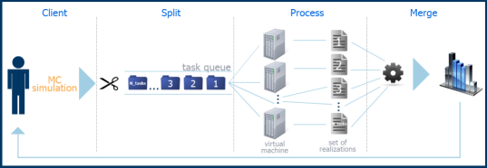
Figure 2: General overview of Monte Carlo parallelization strategy in the cloud.

3.1 Split

First of all, the split step establishes the number of cloud virtual machines to be used and turns then on. Then, it divides a MC simulation with $\displaystyle N_{MC}$ realizations into tasks and puts them into a queue. Each one of these tasks is composed of an ensemble of $\displaystyle N_{serial}$ realizations to be simulated. Thus, it is necessary to process a number of tasks equal to $\displaystyle N_{tasks}=N_{MC}/N_{serial}$. These tasks are distributed in a uniform manner (approximately) among the virtual machines [26, 27]. It is important to note that the number of tasks and virtual machines influences directly in the total simulation processing time and the financial expenses of the cloud computing service.

In the simulations above, the realizations of the random parameters are obtained by the use of a pseudorandom numbers generator. This generator deterministically constructs sequences of numbers indexed by the value of a seed, which emulates a set of random numbers. It happens that, if two instances of tasks have the same seed, they will generate the same sequence of random numbers. In this case, part of these results will be redundant at the end of the simulation.

To avoid the possibility of repeated seeds, it is necessary to adopt a strategy of seed distribution among the virtual machines. This strategy must generate one seed for each virtual machine, and guarantee that the sequence of random numbers generated in each one of these machines is different from the sequences generated on the other machines. There are several ways to define a distribution strategy and we will not discuss this in detail because it is quite simple. To see the strategy adopted in the example of section 5, the reader may consult [26, 27].

3.2 Process

The process step uses the available virtual machines to pick and process, in an asynchronous way, task by task in the queue. Thus, in theory, the execution is as fast as the number of virtual machines used. In practice, there is a limit to efficiency gain because of the existence of overhead, such as input/output of data and managing parallelization. Thus, one of the challenges that must be solved for an efficient simulation, at a low-cost, is the determination of an optimal number of virtual machines to be used [26, 27]. Currently, this optimization process occurs empirically. However, in future works, we will seek to rationalize it, according to the nature of the simulations involved.

At this step, there is a criterion of tolerance against failures. When a task is caught from the queue by a virtual machine, it has a time limit to be executed. If it is not performed in this time, it is put back into the queue for another virtual machine to try and run it. Thus, a hardware or machine communication problem does not overtake the execution of MC simulation.

The output data generated by each executed task is saved onto the hard disk for subsequent post-processing. The total amount of storage space used by a MC simulation is proportional to the number of realizations. Therefore, this step also requires attention in terms of storage space usage because the demand for hard disk space may become unfeasible for a simulation with a large number of realizations.

To reduce the storage space usage in the example of section 5, we chose to calculate the mean and standard deviation using the strategy of pairwise parallel and incremental updates of the statistical moments described in [28], which uses the Welford-Knuth algorithm [29, 30]. Thus, for each executed task, instead of saving all the simulation data for subsequent calculation of the statistical moments, we save only the mean and the centered sum of squares. For the calculation of the histograms, the random variables of interest were identified before the processing step, and their realizations were saved for being used in the histogram construction, during the post-processing step. This strategy is exemplified in Figure 3, which shows the parallelization of a MC simulation, with 16 realizations, that aims to calculate the square of an integer random number between 0 and 9.

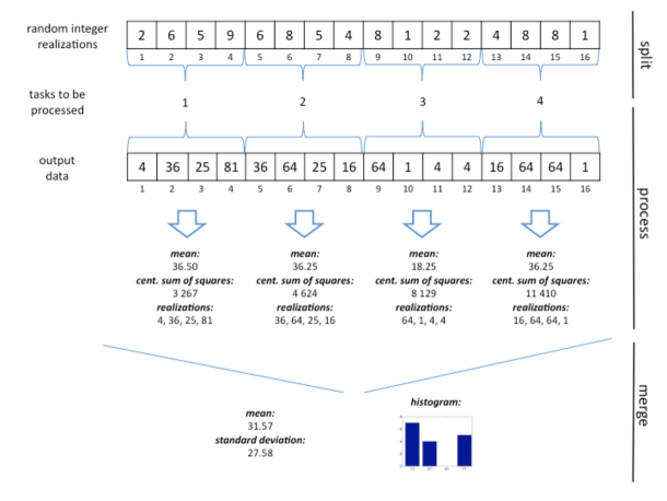
Figure 3: Exemplification of the strategy for parallel calculation of statistics.

3.3 Merge

The merge step starts when the last task in a virtual machine finishes. This can occur in any virtual machine. This step reads, from the hard disk, all the information contained in the output data from the simulations, and combines them through statistics to obtain relevant information about the problem under analysis. At the end of this stage, the saved data are discarded and only the merged result is stored, to reduce future costs of data storage.

4 Case of study

4.1 Physical system

The system of interest in this study case is an elastic bar fixed at a rigid wall, on the left side, and attached to a lumped mass and two springs (one linear and one nonlinear), on the right side, such as illustrated in Figure 4. The stochastic nonlinear dynamics of this system was investigated in [31, 32, 33, 34], where the reader can see more details about the modeling procedure presented below. For simplicity, from now on, this system will be called the fixed-mass-spring bar or simply the bar.

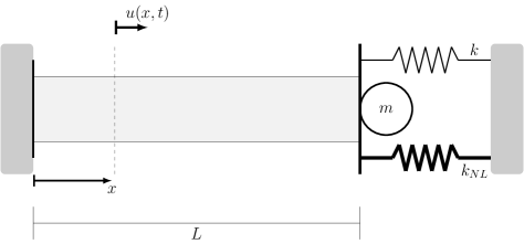
Figure 4: Sketch of a bar fixed at one end and attached to two springs and a mass on the other end.

4.2 Model equation

The physical quantity of interest is the bar displacement field $\displaystyle u$, which depends on the position $\displaystyle x$ and the time $\displaystyle t$, and evolves, for all $\displaystyle(x,t)\in(0,L)\times(0,T)$, according to the following hyperbolic partial differential equation

$$\rho A\mathinner{\dfrac{\partial{{}^{2}}u}{\partial{t^{2}}}}+c\mathinner{\dfrac{\partial{}u}{\partial{t}}}=\mathinner{\dfrac{\partial{}}{\partial{x}}}\left(EA\mathinner{\dfrac{\partial{}u}{\partial{x}}}\right)+f(x,t),$$ (1)

where $\displaystyle\rho$ is mass density, $\displaystyle A$ is the cross section area, $\displaystyle c$ is the damping coefficient, $\displaystyle E$ is the elastic modulus, and $\displaystyle f$ is a distributed external force, which depends on $\displaystyle x$ and $\displaystyle t$.

The boundary conditions for this problem are given by

$$u(0,t)=0,$$ (2)

and

$$EA\mathinner{\dfrac{\partial{}u}{\partial{x}}}(L,t)=-ku(L,t)-k_{NL}\left(u(L,t)\right)^{3}-m\mathinner{\dfrac{\partial{{}^{2}}u}{\partial{t^{2}}}}(L,t),$$ (3)

where $\displaystyle k$ is the stiffness of the linear spring, $\displaystyle k_{NL}$ is the stiffness of the nonlinear spring, and $\displaystyle m$ is the lumped mass.

The initial position and the initial velocity of the bar are

$$u(x,0)=u_{0}(x),$$ (4)

and

$$\mathinner{\dfrac{\partial{}u}{\partial{t}}}(x,0)=v_{0}(x),$$ (5)

where $\displaystyle u_{0}$ and $\displaystyle v_{0}$ are known functions of $\displaystyle x$, defined for $\displaystyle 0\leq x\leq L$.

4.3 Discretization of the model equation

To approximate the solution of the initial/boundary value problem given by Eqs.(1) to (5), we employ the Galerkin method [35]. This results in the following system of ordinary differential equations

$$\left[M\right]\ddot{\mathbf{u}}(t)+\left[C\right]\dot{\mathbf{u}}(t)+\left[K\right]\mathbf{u}(t)=\mathbf{f}(t)+\mathbf{f}_{NL}\left(\dot{\mathbf{u}}(t)\right),$$ (6)

supplemented by the following pair of initial conditions

$$\mathbf{u}(0)=\mathbf{u}_{0}\qquad\mbox{and}\qquad\mathbf{\dot{u}}(0)=\mathbf{v}_{0},$$ (7)

where $\displaystyle\mathbf{u}(t)$ is the vector of $\displaystyle\mathbb{R}^{N}$ in which the $\displaystyle n$-th component is the $\displaystyle u_{n}(t)$, $\displaystyle\left[M\right]$ is the mass matrix, $\displaystyle\left[C\right]$ is the damping matrix, and $\displaystyle\left[K\right]$ is the stiffness matrix. Additionally, $\displaystyle\mathbf{f}(t)$, $\displaystyle\mathbf{f}_{NL}\left(\mathbf{u}(t)\right)$, $\displaystyle\mathbf{u}_{0}$, and $\displaystyle\mathbf{v}_{0}$ are vectors of $\displaystyle\mathbb{R}^{N}$, which respectively represent the external force, the nonlinear force, the initial position, and the initial velocity. The initial value problem defined by Eqs.(6) and (7) has its solution approximated by the Newmark method [36, 35].

4.4 Stochastic model

To introduce randomness in the bar model, we assume that the external force $\displaystyle f$ is a random field proportional to a normalized Gaussian white noise. Moreover, the elastic modulus is assumed to be a random variable.

The probability distribution of $\displaystyle E$ is characterized by its probability density function (PDF) $\displaystyle p_{\tiny{E}}\mathrel{\mathop{\mathchar 58\relax}}(0,\infty)\to\mathbb{R}$, which is specified, based only on the known information about this parameter, by the maximum entropy principle [37, 38, 39, 40].

The maximum entropy principle says that, among all the probability distributions consistent with the current known information of $\displaystyle E$, to choose the one that maximizes its entropy. Thus, to specify $\displaystyle p_{\tiny{E}}$, it is necessary to maximize the entropy function

$$\mathbb{S}\left[p_{\tiny{E}}\right]=-\int_{0}^{\infty}p_{\tiny{E}}(\xi)\ln\left(p_{\tiny{E}}(\xi)\right)d\xi,$$ (8)

subjected to the constraints (known information) imposed by

$$\int_{0}^{\infty}p_{\tiny{E}}(\xi)d\xi=1,$$ (9)

$$\mathbb{E}\left[E\right]=\mu_{E}<\infty,$$ (10)

and

$$\mathbb{E}\left[\ln\left(E\right)\right]<\infty,$$ (11)

where $\displaystyle\mathbb{E}\left[\cdot\right]$ is the expected value operator, and $\displaystyle\mu_{E}$ is the mean value of $\displaystyle E$.

Regarding the known information, the Eq.(9) is the normalization condition of the random variable, the Eq.(10) means that the mean value of $\displaystyle E$ is known, and the Eq.(11) is a sufficient condition to ensure that $\displaystyle U$ have finite variance [37].

The desired distribution is the gamma, whose PDF is given by

$$p_{\tiny{E}}(\xi)=\mathds{1}_{(0,\infty)}\frac{1}{\mu_{E}}\left(\frac{1}{\delta_{E}^{2}}\right)^{\displaystyle\left(\frac{1}{\delta_{E}^{2}}\right)}\frac{1}{\Gamma(1/\delta_{E}^{2})}\left(\frac{\xi}{\mu_{E}}\right)^{\displaystyle\left(\frac{1}{\delta_{E}^{2}}-1\right)}\exp\left(-\frac{\xi}{\delta_{E}^{2}\mu_{E}}\right),$$ (12)

where the symbol $\displaystyle\mathds{1}_{(0,\infty)}$ denotes the indicator function of the interval $\displaystyle(0,\infty)$, $\displaystyle\delta_{E}$ is a dispersion factor, and the $\displaystyle\Gamma$ indicates the gamma function.

Due to the randomness of $\displaystyle F$ and $\displaystyle E$, the displacement of the bar becomes a random field $\displaystyle U$, which evolves according to the following stochastic partial differential equation

$$\rho A\mathinner{\dfrac{\partial{{}^{2}}U}{\partial{t^{2}}}}+c\mathinner{\dfrac{\partial{}U}{\partial{t}}}=\mathinner{\dfrac{\partial{}}{\partial{x}}}\left(E(\theta)A\mathinner{\dfrac{\partial{}U}{\partial{x}}}\right)+F(x,t,\theta).$$ (13)

The boundary conditions now read as

$$U(0,t,\theta)=0,$$ (14)

and

$$EA\mathinner{\dfrac{\partial{}U}{\partial{x}}}(L,t,\theta)=-kU(L,t,\theta)-k_{NL}\left(U(L,t,\theta)\right)^{3}-m\mathinner{\dfrac{\partial{{}^{2}}U}{\partial{t^{2}}}}(L,t,\theta),$$ (15)

for $\displaystyle 0<t<T$ and $\displaystyle\theta\in\SS$, while the initial conditions are

$$U(x,0,\theta)=u_{0}(x),$$ (16)

and

$$\mathinner{\dfrac{\partial{}U}{\partial{t}}}(x,0,\theta)=v_{0}(x),$$ (17)

for $\displaystyle 0\leq x\leq L$ and $\displaystyle\theta\in\SS$, where $\displaystyle\SS$ denotes the sample space in which we are working.

5 Numerical experiments

We employ the MC method in the cloud to approximate the solution of the stochastic initial/boundary value problem defined by Eqs.(13) to (17). This procedure uses a sampling strategy with the number of realizations always being equal to a power of four. In this procedure, each realization of the random parameters defines a new initial value problem given by Eqs.(6) and (7), which is solved deterministically as described in section 4.3. Then, these results are combined through statistics.

The implementation of the MC method was conducted in MATLAB, with the aid of two executable files. The first one, which is executed in each one of the virtual machines, generates realizations of the random parameters and performs the determinist calculations to solve the associated variational problem. The other executable computes the statistics of the output data generated by the first executable.

5.1 Probability density function

A random variable is completely characterized by its PDF. The knowledge of the PDF allows us to obtain all the statistical moments of the random variable and to calculate the probability of any event associated with it. So, we start our analysis with the PDF estimation.

The estimations for the PDF of the (normalized) bar right extreme displacement for a fixed instant of time, is shown in Figure 5 for different values of the total number of realizations in MC simulations. We can note that as the number of samples in the MC simulation increases, small differences may be noted on the peaks of successive estimations of the PDF.

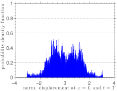
(a) $\displaystyle 16,384$ realizations

(b) $\displaystyle 65,536$ realizations

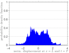
(c) $\displaystyle 262,144$ realizations

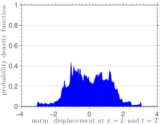
(d) $\displaystyle 1,048,576$ realizations

Figure 5: This Figure illustrates estimations for the PDF of the (normalized) random variable $\displaystyle U(L,T,\cdot)$, for different values of the total number of realizations in MC simulations: (a) $\displaystyle 16,384$ realizations, (b) $\displaystyle 65,536$ realizations, (c) $\displaystyle 262,144$ realizations and (d) $\displaystyle 1,048,576$ realizations.

We use a convergence criterion based on a residue of the random variable $\displaystyle U(L,T,\theta)$, defined as the absolute value of the difference between two successive approximations of $\displaystyle p_{\tiny{U(L,T,\cdot)}}$, i.e.,

$$R_{U(L,T,\cdot)}=\left|p_{\tiny{U(L,T,\cdot)}}^{4n}-p_{\tiny{U(L,T,\cdot)}}^{n}\right|,$$ (18)

where the superscript $\displaystyle n$ indicates the number of realizations in the MC simulation. In this case, we say that the MC simulation reached a satisfactory result if this residue is less than a prescribed tolerance $\displaystyle\epsilon$, i.e., $\displaystyle R_{U(L,T,\cdot)}<\epsilon$ for all $\displaystyle\theta\in\SS$. For instance, $\displaystyle\epsilon=0.05$.

The reader can observe the distribution of the residue of $\displaystyle U(L,T,\theta)$, for several values of MC realizations, in the Figure 6. Note that although the residue decreases with the increase of the MC realizations, only one simulation with $\displaystyle 1,048,576$ samples was able to fulfill the convergence criterion.

Therefore, despite the number of samples used in the MC simulation is very high and the problem is relatively simple, the tolerance achieved was relatively low. It is common to observe in the literature some works that analyze problems much more complex, for instance [41, 42, 43], among many others, using some hundreds of samples.

This example leads us to reflect about the number of realizations required to obtain statistical independence of the results. In this context, the use of MC in a cloud computing setting appears to be a viable solution, able to make the work feasible at a low-cost.

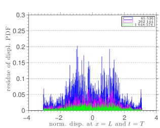
Figure 6: This figure illustrates the residue of the $\displaystyle U(L,T,\cdot)$ PDF.

5.2 Mean and standard deviation

Figure 7 shows the evolution of the bar right extreme displacement mean (blue line) and an envelope of reliability (grey shadow) around it, obtained by adding and subtracting one standard deviation around the mean. This figure shows these graphs for different values of the total number of realizations in MC simulations.

The first conclusion we can draw from these results is that the low-order statistics, from the qualitative point of view, do not undergo major changes when the total number of realizations is higher than $\displaystyle 16,384$. However, based on a purely visual analysis, we can not conclude anything quantitatively.

(a) $\displaystyle 16,384$ realizations

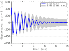
(b) $\displaystyle 65,536$ realizations

(c) $\displaystyle 262,144$ realizations

(d) $\displaystyle 1,048,576$ realizations

Figure 7: This Figure illustrates the mean value (blue line) and a confidence interval (grey shadow) with one standard deviation, of the random process $\displaystyle U(L,\cdot,\cdot)$, for different values of the total number of realizations in MC simulations: : (a) $\displaystyle 16,384$ realizations, (b) $\displaystyle 65,536$ realizations, (c) $\displaystyle 262,144$ realizations and (d) $\displaystyle 1,048,576$ realizations.

To investigate the quantitative differences on the results, we define the residue of $\displaystyle U(L,\cdot,\cdot)$ mean or standard deviation similarly to the one defined to Eq.(18), by changing the PDF for the mean or standard deviation of $\displaystyle U(L,\cdot,\cdot)$ only.

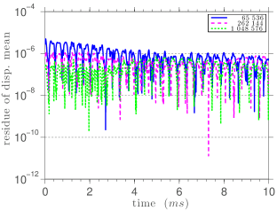
Figure 8: This figure illustrates the evolution of residue of the $\displaystyle U(L,\cdot,\cdot)$ mean.

Figure 8 illustrates the evolution of several residues of the $\displaystyle U(L,\cdot,\cdot)$ mean, and Figure 9 illustrates the evolution of several residues of the $\displaystyle U(L,\cdot,\cdot)$ standard deviation. We note that, the logarithm of the mean value residues are almost always less than $\displaystyle\mathcal{O}(10^{-6})$, for the case of statistics with larger samples, and presents an alternate behavior between large drops and climbs, (as seen in Figure 8). On the other hand, the logarithm of the standard deviation residue is greater than $\displaystyle\mathcal{O}(10^{-6})$ in the initial instants. This behavior is not maintained after $\displaystyle 2~{}ms$, when the residue curves keep their alternate behavior, but almost always below $\displaystyle\mathcal{O}(10^{-6})$, as shown in Figure 9. These results show that statistics of first and second order may be obtained with great accuracy using the methodology presented in this work.

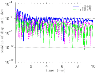
Figure 9: This figure illustrates the evolution of the residue of the $\displaystyle U(L,\cdot,\cdot)$ standard deviation.

5.3 Costs analysis for the processing time

In what follows we will present an evaluation of the time spent by MC simulations based on the number of realizations. All the simulations were performed only once, without discarding any samples. Also, 20 virtual machines were used for the experiment, one for control and the other 19 for processing. Each task runned uses $\displaystyle N_{serial}=256$.

Table 1: Comparison between the computational time spent (using 19 VMs) by each one of the MC simulations in the cloud, and the corresponding speed-up factors compared to a serial simulation.

$\displaystyle N_{MC}$	tasks	split	process	merge	total	serial	speed-up
		(ms)	(ms)	(ms)	(min)	(min)
256	1	—	111 998	2 250	1.9	1.9	1.0
16 384	64	500	451 397	11 875	7.7	127.3	16.5
65 536	256	2 328	1 576 711	27 031	26.7	509.3	19.0
262 144	1024	7 609	6 078 757	89 450	102.9	2 037.0	19.8
1 048 576	4096	37 766	24 422 238	336 799	413.3	8 148.1	19.7

A comparison between the computational time spent by each one of the MC simulations in the cloud, and the corresponding speed-up factors compared with a serial simulation can be seen in the Table 1. In this table the column $\displaystyle N_{MC}$ represents the total number of realizations of the experiment; the column tasks represents the number of tasks to be processed; the columns split, process and merge represent the time, in milliseconds, consumed in each stage of our parallelization strategy; the column total represents, in minutes, the total time spent by the parallel MC simulation (split + process + merge); the column serial shows, in minutes, the processing time of a MC simulation for the same problem executed in serial; and the column speed-up shows a metric of the parallel simulation performance, defined as the ratio between the serial and the total time of simulation.

Before discussing the analysis of the results, we should indicate that the serial time, shown in the first line of the Table 1, was obtained by extrapolation of the average processing time spent to run a single task in two virtual machines of the cloud. To obtain this average time the task was repeated 10 times (5 times in each VM).

The first thing that we can note in the Table 1 is that the computational cost of the split and merge tasks are almost negligible when compared to the time spent by the process. Hence the importance of adopting a strategy of parallelism for the processing step. Also, we can see that, in all of the experiments, the strategy of parallelism in the cloud provided performance gains, and such gains are greater as the number of realizations increases. This shows the efficiency of our parallelization strategy in the case of study analyzed. Moreover, the speed-up observed is close to the number of virtual machines used, which indicates that the implementation of the McCloud setting is good.

In order to evaluate the efficiency of the parallelization done in the cloud, we studied how the processing time of the MC simulation, with $\displaystyle 1,048,576$ realizations, varies as a function of the number of virtual machines used to perform the task. As can be seen in the Table 2, the processing time decays monotonically as the number of VMs increases. This decreasing behavior is almost linear in logarithmic scale, as shown in the Figure 10, and indicates the effectiveness of the parallelization of MC tasks in the cloud.

Table 2: Comparison between the computational time spent (using 19 VMs) by each one of the MC simulations in the cloud, and the corresponding speed-up factors compared to a serial simulation.

VMs	split	process	merge	total	speed-up	cost
	(ms)	(ms)	(ms)	(min)		(US$)
4	37 734	117 637 861	431 691	1968.5	4.0	17.15
5	34 062	99 041 631	354 791	1657.2	4.7	18.23
6	37 923	78 040 047	343 105	1307.0	6.0	17.39
7	36 982	66 989 658	348 603	1122.9	7.0	17.63
8	27 390	58 431 244	349 099	980.1	8.0	18.11
9	29 407	51 818 238	343 720	869.9	9.0	18.11
10	28 015	46 564 270	332 119	782.1	10.0	18.83
11	28 734	42 192 535	334 432	709.3	11.0	17.99
12	27 687	38 611 499	341 308	649.7	12.0	18.11
13	34 874	36 039 896	334 806	606.8	12.9	19.55
14	36 359	33 412 517	338 696	563.1	13.9	19.31
15	36 499	31 199 806	343 874	526.3	14.8	18.83
16	38 576	29 215 641	338 014	493.2	15.8	20.03
17	40 484	27 406 752	340 522	463.1	16.8	19.19
18	39 015	25 800 653	335 214	436.3	17.9	20.27
19	37 766	24 422 238	336 799	413.3	18.9	19.07
29	29 282	16 000 466	343 036	272.9	28.6	21.71
39	29 547	11 927 263	346 594	205.1	38.0	24.23
60	31 547	7 891 904	327 392	137.5	56.7	29.63
80	25 328	5 900 347	33 709	99.3	78.5	29.63
99	29 578	4 834 623	340 015	86.7	89.9	36.47

The small deviations from the theoretical curve of parallelization, that can be seen in the Figure 10, are due to the management of tasks by the cloud. However, in the range analyzed, between 4 and 99 virtual machines, these performance losses are negligible and do not compromise the efficiency of parallelization strategy.

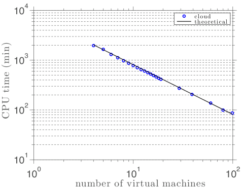
Figure 10: CPU time of a MC simulation, with 1 048 576 realizations, as function of the numbers of virtual machines.

Table 2 also shows that the speed-up increases monotonically as the number of VMs grows. This behavior can be better appreciated in the Figure 11, where the reader can verify that the values obtained for the speed-up are very close to the theoretical values, that would be obtained if there were no delays due to cloud management. The reader can note, also, that the measured values The ​corresponding to larger numbers of VMs (60, 80 and 99) are farther away from the theoretical reference. This occurs by the accumulation of management delays, which are larger for a higher amount of VMs.

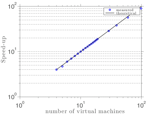
Figure 11: Speed-up of a MC simulation, with 1 048 576 realizations, as function of the numbers of virtual machines.

5.4 Costs analysis for the storage space

A comparison between the storage space used by each one of the MC simulations in the cloud, and the financial cost associated with each simulation can be seen in Table 3. In this table the column space represents the total storage space, in $\displaystyle MB$, temporarily used by the simulation, and the column cost represents the cost of this experiment in US dollars.

Table 3: Comparison between the storage space used by each one of the MC simulations in the cloud, and the financial cost associated with each simulation.

$\displaystyle N_{MC}$	space	cost
	($\displaystyle MB$)	($\displaystyle US\$$)
16 384	12.4	5.39
65 536	49.0	5.39
262 144	195.2	7.67
1 048 576	780.8	19.07

Observing the data in Table 3 we can see that our parallelization strategy used fairly little storage space, even for a large number of MC realizations. Additionally, the financial cost, even for the most complex simulation, is very small; which is a major advantage when compared to the costs of acquiring and maintaining a traditional cluster.

6 Concluding remarks

We present a strategy for parallelizing the Monte Carlo method in the context of cloud computing, using the fundamental idea of the MapReduce paradigm. This strategy is described in detail and illustrated in the simulation of a simple problem of stochastic structural dynamics. The simulation results show good accuracy for low-order statistics, low storage space usage, and that the performance gains increase with the number of Monte Carlo realizations. It was also illustrated that even a simple problem can require many realizations for the convergence of histograms, which makes the cloud computing strategy very attractive, due to its high scalability capacity and low-cost. Thus, this article demonstrates that the advent of cloud computing can become an important enabler for the adoption of the MC method to compute the propagation of uncertainty in complex stochastic models.

References

- [1] C. Soize, Random matrix theory for modeling uncertainties in computational mechanics, Computer Methods in Applied Mechanics and Engineering 194 (2005) 1333–1366. doi:10.1016/j.cma.2004.06.038.
- [2] T. G. Ritto, R. Sampaio, Stochastic drill-string dynamics with uncertainty on the imposed speed and on the bit-rock parameters, International Journal for Uncertainty Quantification 2 (2012) 111–124. doi:10.1615/Int.J.UncertaintyQuantification.v2.i2.
- [3] T. G. Ritto, M. R. Escalante, R. Sampaio, M. B. Rosales, Drill-string horizontal dynamics with uncertainty on the frictional force, Journal of Sound and Vibration 332 (2013) 145–153. doi:10.1016/j.jsv.2012.08.007.
- [4] T. G. Ritto, C. Soize, R. Sampaio, Non-linear dynamics of a drill-string with uncertain model of the bit rock interaction, International Journal of Non-Linear Mechanics 44 (2009) 865–876. doi:10.1016/j.ijnonlinmec.2009.06.003.
- [5] T. G. Ritto, R. Sampaio, F. Rochinha, Model uncertainties of flexible structures vibrations induced by internal flows, Journal of the Brazilian Society of Mechanical Sciences and Engineering 33 (2011) 373–380. doi:10.1590/S1678-58782011000300014.
- [6] S. Zio, F. Rochinha, A stochastic collocation approach for uncertainty quantification in hydraulic fracture numerical simulation, International Journal for Uncertainty Quantification 2 (2012) 145–160. doi:10.1615/Int.J.UncertaintyQuantification.v2.i2.
- [7] H. Lopes, J. Barcellos, J. Kubrusly, C. Fernandes, A non-parametric method for incurred but not reported claim reserve estimation, International Journal for Uncertainty Quantification 2 (2012) 39–51. doi:10.1615/Int.J.UncertaintyQuantification.v2.i1.40.
- [8] A. Clément, C. Soize, J. Yvonnet, Uncertainty quantification in computational stochastic multiscale analysis of nonlinear elastic materials, Computer Methods in Applied Mechanics and Engineering 254 (2013) 61–82. doi:10.1016/j.cma.2012.10.016.
- [9] C. Soize, A comprehensive overview of a non-parametric probabilistic approach of model uncertainties for predictive models in structural dynamics, Journal of Sound and Vibration 288 (2005) 623–652. doi:10.1016/j.jsv.2005.07.009.
- [10] C. Soize, Stochastic modeling of uncertainties in computational structural dynamics - Recent theoretical advances, Journal of Sound and Vibration 332 (2013) 2379––2395. doi:10.1016/j.jsv.2011.10.010.
- [11] N. Metropolis, S. Ulam, The Monte Carlo Method, Journal of the American Statistical Association 44 (1949) 335–341. doi:10.2307/2280232.
- [12] J. S. Liu, Monte Carlo Strategies in Scientific Computing, Springer, New York, 2001.
- [13] R. W. Shonkwiler, F. Mendivil, Explorations in Monte Carlo Methods, Springer, New York, 2009.
- [14] C. P. Robert, G. Casella, Monte Carlo Statistical Methods, Springer, New York, 2010.
- [15] D. Xiu, G. E. Karniadakis, The Wiener-Askey Polynomial Chaos for stochastic differential equations, SIAM Journal on Scientific Computing 24 (2002) 619–644. doi:10.1137/S1064827501387826.
- [16] J. Dean, S. Ghemawat, MapReduce: Simplified data processing on large clusters, in: OSDI, 2004.
- [17] J. Shiers, Grid today, clouds on the horizon, Computer Physics Communications 180 (2009) 559–563. doi:10.1016/j.cpc.2008.11.027.
- [18] I. Ari, N. Muhtaroglu, Design and implementation of a cloud computing service for finite element analysis, Advances in Engineering Software 60-61 (2013) 122–135. doi:10.1016/j.advengsoft.2012.10.003.
- [19] K. Jorissen, F. Vila, J. J. Rehr, A high performance scientific cloud computing environment for materials simulations, Computer Physics Communications 183 (2012) 1911–1919. doi:10.1016/j.cpc.2012.04.010.
- [20] L. Wang, M. Kunze, J. Tao, G. von Laszewski, Towards building a cloud for scientific applications, Advances in Engineering Software 42 (2011) 714–722. doi:10.1016/j.advengsoft.2011.05.007.
- [21] T. Velte, A. Velte, R. Elsenpeter, Cloud Computing, A Practical Approach, McGraw-Hill Osborne Media, New York, 2009.
- [22] D. Cearley, Hype Cycle for Application Development, Tech. Rep. G00147982, Gartner Group (2009).
- [23] L. M. Vaquero, L. Rodero-Merino, J. Caceres, M. Lindner, A break in the clouds: towards a cloud definition, Computer Communication Review 39 (2008) 50–55.
- [24] R. Buyya, J. Broberg, A. M. Goscinski, Cloud computing: Principles and paradigms.
- [25] E. Roloff, M. Diener, A. Carissimi, P. O. A. Navaux, High performance computing in the cloud: Deployment, performance and cost efficiency, in: Cloud Computing Technology and Science (CloudCom), 2012 IEEE 4th International Conference on, 2012, pp. 371–378. doi:10.1109/CloudCom.2012.6427549.
- [26] R. Nasser, McCloud Service Framework: Development Services of Monte Carlo Simulation in the Cloud, M.Sc. Dissertation, Pontifícia Universidade Católica do Rio de Janeiro, Rio de Janeiro, (in portuguese) (2012).
- [27] R. Nasser, A. Cunha Jr, H. Lopes, K. Breitman, R. Sampaio, McCloud: Easy and quick way to run Monte Carlo simulations in the cloud, (submitted for publication) (2013).
- [28] J. Bennett, R. Grout, P. Pebay, D. Roe, D. Thompson, Numerically stable, single-pass, parallel statistics algorithms, in: IEEE International Conference on Cluster Computing and Workshops 2009, 2009. doi:10.1109/CLUSTR.2009.5289161.
- [29] B. P. Welford, Note on a method for calculating corrected sums of squares and products, Technometric 4 (1962) 419–420. doi:10.1080/00401706.1962.10490022.
- [30] D. E. Knuth, The Art of Computer Programming, volume 2: Seminumerical Algorithms, 3rd Edition, Addison-Wesley, Boston, 1998.
- [31] A. Cunha Jr, R. Sampaio, Effect of an attached end mass in the dynamics of uncertainty nonlinear continuous random system, Mecánica Computacional 31 (2012) 2673–2683.
- [32] A. Cunha Jr, R. Sampaio, Uncertainty propagation in the dynamics of a nonlinear random bar, in: Proceedings of the XV International Symposium on Dynamic Problems of Mechanics, 2013.
- [33] A. Cunha Jr, R. Sampaio, Analysis of the nonlinear stochastic dynamics of an elastic bar with an attached end mass, in: Proceedings of the III South-East Conference on Computational Mechanics, 2013.
- [34] A. Cunha Jr, R. Sampaio, On the nonlinear stochastic dynamics of a continuous system with discrete attached elements, (submitted for publication) (2013).
- [35] T. J. R. Hughes, The Finite Element Method, Dover Publications, New York, 2000.
- [36] N. Newmark, A method of computation for structural dynamics, Journal of the Engineering Mechanics Division 85 (1959) 67–94.
- [37] C. Soize, A nonparametric model of random uncertainties for reduced matrix models in structural dynamics, Probabilistic Engineering Mechanics 15 (2000) 277 – 294. doi:10.1016/S0266-8920(99)00028-4.
- [38] C. Shannon, A mathematical theory of communication, Bell System Technical Journal 27 (1948) 379– 423.
- [39] E. T. Jaynes, Information theory and statistical mechanics, Physical Review Series II 106 (1957) 620–630. doi:10.1103/PhysRev.106.620.
- [40] E. T. Jaynes, Information theory and statistical mechanics II, Physical Review Series II 108 (1957) 171–190. doi:10.1103/PhysRev.108.171.
- [41] P. Spanos, A. Kontsos, A multiscale Monte Carlo finite element method for determining mechanical properties of polymer nanocomposites, Probabilistic Engineering Mechanics 23 (2008) 456–470. doi:10.1016/j.probengmech.2007.09.002.
- [42] B. Liang, S. Mahadevan, Error and uncertainty quantification and sensitivity analysis in mechanics computational models, International Journal for Uncertainty Quantification 1 (2011) 147–161. doi:10.1615/IntJUncertaintyQuantification.v1.i2.30.
- [43] S. Murugan, R. Chowdhury, S. Adhikari, M. Friswell, Helicopter aeroelastic analysis with spatially uncertain rotor blade properties, Aerospace Science and Technology 16 (2012) 29 –39. doi:10.1016/j.ast.2011.02.004.