Physics-informed neural networks (PINNs) for fluid mechanics: A review

Abstract

Despite the significant progress over the last 50 years in simulating flow problems using numerical discretization of the Navier-Stokes equations (NSE), we still cannot incorporate seamlessly noisy data into existing algorithms, mesh-generation is complex, and we cannot tackle high-dimensional problems governed by parametrized NSE. Moreover, solving inverse flow problems is often prohibitively expensive and requires complex and expensive formulations and new computer codes. Here, we review flow physics-informed learning, integrating seamlessly data and mathematical models, and implementing them using physics-informed neural networks (PINNs). We demonstrate the effectiveness of PINNs for inverse problems related to three-dimensional wake flows, supersonic flows, and biomedical flows.

1 Introduction

In the last 50 years there has been a tremendous progress in computational fluid dynamics (CFD) in solving numerically the incompressible and compressible Navier-Stokes equations (NSE) using finite elements, spectral, and even meshless methods brooks1982streamline ; GK_CFDbook ; katz2009meshless ; liu2010smoothed . Yet, for real-world applications, we still cannot incorporate seamlessly (multi-fidelity) data into existing algorithms, and for industrial-complexity problems the mesh generation is time consuming and still an art. Moreover, solving inverse problems, e.g., for unknown boundary conditions or conductivities beck1985inverse , etc., is often prohibitively expensive and requires different formulations and new computer codes. Finally, computer programs such as OpenFOAM jasak2007openfoam have more than 100,000 lines of code, making it almost impossible to maintain and update them from one generation to the next.

Physics-informed learning raissi2021physics , introduced in a series of papers by Karniadakis’s group both for Gaussian-process regression raissi2017machine ; raissi2018numerical and physics-informed neural networks (PINNs) raissi2019deep , can seamlessly integrate multifidelity/multimodality experimental data with the various Navier-Stokes formulations for incompressible flows jin2021nsfnets ; raissi2020hidden as well as compressible flows mao2020physics and biomedical flows yin2021non . PINNs use automatic differentiation to represent all the differential operators and hence there is no explicit need for a mesh generation. Instead, the Navier-Stokes equations and any other kinematic or thermodynamic constraints can be directly incorporated in the loss function of the neural network (NN) by penalizing deviations from the target values (e.g., zero residuals for the conservation laws) and are properly weighted with any given data, e.g., partial measurements of the surface pressure. PINNs are not meant to be a replacement of the existing CFD codes, and in fact the current generation of PINNs is not as accurate or as efficient as high-order CFD codes GK_CFDbook for solving the standard forward problems. This limitation is associated with the minimization of the loss function, which is a high-dimensional non-convex function, a limitation which is a grand challenge of all neural networks for even commercial machine learning. However, PINNs perform much more accurately and more efficiently than any CFD solver if any scattered partial spatio-temporal data are available for the flow problem under consideration. Moreover, the forward and inverse PINN formulations are identical so there is no need for expensive data assimilation schemes that have stalled progress especially for optimization and design applications of flow problems in the past.

In this paper we first review the basic principles of PINNs and recent extensions using domain decomposition for multiphysics and multiscale flow problems. We then present new results for a three-dimensional (3D) wake formed in incompressible flow behind a circular cylinder. We also show results for a two-dimensional (2D) supersonic flow past a blunt body, and finally we infer material parameters in simulating thrombus deformation in a biomedical flow.

2 PINNs: Physics-Informed Neural Networks

In this section we first review the basic PINN concept and subsequently discuss more recent advancements in incompressible, compressible and biomedical flows.

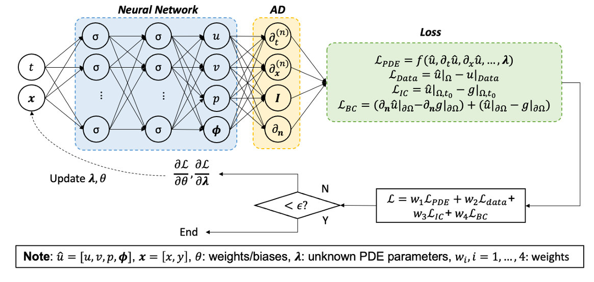
Figure 1: Schematic of a physics-informed neural network (PINN). A fully-connected neural network, with time and space coordinates ($t,\mathbf{x}$) as inputs, is used to approximate the multi-physics solutions $\hat{u}=[u,v,p,\phi]$. The derivatives of $\hat{u}$ with respect to the inputs are calculated using automatic differentiation (AD) and then used to formulate the residuals of the governing equations in the loss function, that is generally composed of multiple terms weighted by different coefficients. The parameters of the neural network $\theta$ and the unknown PDE parameters $\lambda$ can be learned simultaneously by minimizing the loss function.

2.1 PINNs: Basic Concepts

We consider a parametrized partial differential equation (PDE) system given by:

$$f(\mathbf{x},t,\hat{u},\partial_{\mathbf{x}}\hat{u},\partial_{t}\hat{u},\dots,\bm{\lambda})=0,\quad\mathbf{x}\in\Omega,~{}t\in[0,T]$$ (1)

$$\hat{u}(\mathbf{x},t_{0})=g_{0}(\mathbf{x})\quad\mathbf{x}\in\Omega,$$

$$\hat{u}(\mathbf{x},t)=g_{\Gamma}(t),\quad\mathbf{x}\in\partial\Omega,~{}t\in[0,T],$$

where $\mathbf{x}\in\mathbb{R}^{d}$ is the spatial coordinate and $t$ is the time; $f$ denotes the residual of the PDE, containing the differential operators (i.e., $[\partial_{\mathbf{x}}\hat{u},\partial_{t}\hat{u},\dots]$); $\bm{\lambda}=[\lambda_{1},\lambda_{2},\dots]$ are the PDE parameters; $\hat{u}(\mathbf{x},t)$ is the solution of the PDE with initial condition $g_{0}(\mathbf{x})$ and boundary condition $g_{\Gamma}(t)$ (which can be Dirichlet, Neumann or mixed boundary condition); $\Omega$ and $\partial\Omega$ represent the spatial domain and the boundary, respectively.

In the context of the vanilla PINNs raissi2019physics , a fully-connected feed-forward neural network, which is composed of multiple hidden layers, is used to approximate the solution of the PDE $\hat{u}$ by taking the space and time coordinates $(\mathbf{x},t)$ as inputs, as shown in the blue panel in Fig. 1. Let the hidden variable of the $k^{th}$ hidden layer be denoted by $\mathbf{z}^{k}$, then the neural network can be expressed as

$$\mathbf{z}^{0}=(\mathbf{x},t),$$ (2)

$$\mathbf{z}^{k}=\sigma(\mathbf{W}^{k}\mathbf{z}^{k-1}+\mathbf{b}^{k}),\quad 1\leq k\leq L-1$$

$$\mathbf{z}^{k}=\mathbf{W}^{k}\mathbf{z}^{k-1}+\mathbf{b}^{k},\quad k=L,$$

where the output of the last layer is used to approximate the true solution, namely $\hat{u}\approx\mathbf{z}^{L}$. $\mathbf{W}^{k}$ and $\mathbf{b}^{k}$ denote the weight matrix and bias vector of the $k^{th}$ layer; $\sigma(\cdot)$ is a nonlinear activation function. All the trainable model parameters, i.e., weights and biases, are denoted by $\theta$ in this paper.

In PINNs, solving a PDE system (denoted by equ. 1) is converted into an optimization problem by iteratively updating $\theta$ with the goal to minimize the loss function $L$:

$$L=\omega_{1}L_{PDE}+\omega_{2}L_{data}+\omega_{3}L_{IC}+\omega_{4}L_{BC},$$ (3)

where $\omega_{1-4}$ are the weighting coefficients for different loss terms. The first term $L_{PDE}$ in equ. 3 penalizes the residual of the governing equations. The other terms are imposed to satisfy the model predictions for the measurements $L_{data}$, the initial condition $L_{IC}$, and the boundary condition $L_{BC}$, respectively. In general, the mean square error (MSE), taking the $L_{2}$-norm of the sampling points, is employed to compute the losses in equ. 3. The sampling points are defined as a data set $\{\mathbf{x}^{i},t^{i}\}_{i=1}^{N}$, where the number of points (denoted by $N$) for different loss terms can be different. Generally, we use the ADAM optimizer kingma2014adam , an adaptive algorithm for gradient-based first-order optimization, to optimize the model parameters $\theta$.

Remark 1: We note that the definition of the loss function shown in equ. 3 is problem-dependent, hence some terms may disappear for different types of the problem. For example, when we solve a forward problem in fluid mechanics with the known parameters ($\mathbf{\lambda}$) and the initial/boundary conditions of the PDEs, the data loss $L_{data}$ is not necessarily required. However, in the cases where the model parameters or the initial/boundary conditions are unknown (namely, inverse problems), the data measurements should be taken into account in order to make the optimization problem solvable. We also note that the PINN framework can be employed to solve an “over-determined” system, e.g., well-posed in a classical sense with initial and boundary conditions known and additionally some measurements inside the domain or at boundaries (e.g., pressure measurements).

One of the key procedures to construct the PDE loss in equ. 3 is the computation of partial derivatives, which is addressed by using automatic differentiation (AD). Relying on the combination of the derivatives for a sequence of operations by using the chain rule, AD calculates the derivatives of the outputs with respect to the network inputs directly in the computational graph. The computation of partial derivatives can be calculated with an explicit expression, hence avoiding introducing truncation errors in conventional numerical approximations. At the present time, AD has been implemented in various deep learning frameworks abadi2016tensorflow ; paszke2019pytorch , which makes it convenient for the development of PINNs.

A schematic of PINNs is shown in Fig. 1, where the key elements (e.g., neural network, AD, loss function) are indicated in different colors. Here, we consider a multi-physics problem, where the solutions include the velocity $(u,v)$, pressure $p$ and a scalar field $\phi$, which are coupled in a PDE system $f$. The schematic in Fig. 1 represents most of the typical problems in fluid mechanics. For instance, the PDEs considered here can be the Boussinesq approximation of the Navier-Stokes equations, where $\phi$ is the temperature. Following the paradigm in Fig. 1, we will describe the governing equations, the loss function and the neural network configurations of PINNs case-by-case in the rest of this paper.

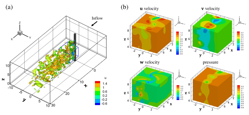
Figure 2: Case study of PINNs for incompressible flows: illustration of simulating the 3D wake flow over a circular cylinder. (a) Iso-surface of the vorticity (x-component) in the whole domain color-coded by the streamwise velocity. The cube with blue edges represents the computational domain in this case. (b) Velocity and pressure fields in the domain. The simulation was performed by the CFD solver Nektar, which is based on the spectral/hp element method GK_CFDbook .

2.2 Recent Advances of PINNs

First proposed in raissi2017physicsA ; raissi2017physicsB , see also raissi2019physics , PINNs have attracted a lot of attention in the scientific computing community as well as the fluid mechanics community. Here, we review some related works regarding the methodology and the application to fluid mechanics.

Beneficial due to the high flexibility and the expressive ability in function approximation, PINNs have been extended to solve various classes of PDEs, e.g., integro-differential equations pang2019fpinns , fractional equations pang2019fpinns , surfaces PDEs fang2019physics and stochastic differential equations zhang2020learning . A variational formulation of PINNs based on the Galerkin method (hp-VPINN) was proposed to deal with PDEs with non-smooth solutions kharazmi2021hp . In addition, the variational hp-VPINN considered domain decomposition, and similar pointwise versions were also studied in CPINN jagtap2020conservative , and XPINN jagtap2020extended . A general parallel implementation of PINNs with domain decomposition for flow problems is presented in shukla2021parallel ; the NVIDIA library SimNet hennigh2020nvidia is also a very efficient implementation of PINNs. Another important extension is the uncertainty quantification for the PDE solutions inferred by neural networks yang2019adversarial ; zhang2019quantifying ; ZhuZabKouPer2019JCP ; sun2020physics ; yang2021bpinns . This has been studied by using the Bayesian framework yang2021bpinns . Moreover, some other researches on PINNs focused on the development of the neural network architecture and the training, e.g., using multi-fidelity framework meng2020composite , adaptive activation functions jagtap2020adaptive and dynamic weights of the loss function wang2020understanding , hard constraints lu2021physics and CNN-based network architectures gao2021phygeonet , which can improve the performance of PINNs on different problems. On the theoretical side, some recent works shin2020convergence ; mishra2020estimates ; wang2020when have provided more guarantees and insights into the convergence of PINNs.

The development of the methodology has inspired a number of applications in other fields, especially in fluid mechanics where the flow phenomena can be described by the NSE. In raissi2019physics , the vanilla PINN was proposed to infer the unknown parameters (e.g., the coefficient of the convection term) in the NS equations based on velocity measurements for the 2D flow over a cylinder. Following this work, PINNs were then applied to various flows raissi2019deep ; jin2021nsfnets ; raissi2020hidden ; mao2020physics ; yin2021non ; kissas2020machine ; yang2019predictive ; lou2020physics ; cai2021physics ; cai2021flow ; wang2021deep ; lucor2021physics ; mahmoudabadbozchelou2021data , covering the applications on compressible flows mao2020physics , biomedical flows yin2021non ; kissas2020machine ; arzani2021uncovering , turbulent convection flows lucor2021physics , free boundary and Stefan problems wang2021deep , etc. The main attractive advantage of PINNs in solving fluid mechanics problems is that a unified framework (shown in Fig. 1) can be used for both forward and inverse problems. Compared to the traditional CFD solvers, PINNs are superior at integrating the data (observations of the flow quantities) and physics (governing equations). A promising application is on the flow visualization technology raissi2020hidden ; cai2021artificial , where the flow fields can be easily inferred from the observations such as concentration fields and images. On the contrary, such inverse problems are difficult for conventional CFD solvers. More relevant works on mechanics in general can be found in wang2020towards for turbulent flow, goswami2020transfer for phase-field fracture model, and zhang2020physics for inferring modulus in a nonhomogeneous material.

3 Case Study for 3D Incompressible Flows

In this section, we demonstrate the effectiveness of PINNs for solving inverse problems in incompressible flows. In particular, we apply PINNs to reconstruct the 3D flow fields based on a few two-dimensional and two-component (2D2C) velocity observations. The proposed algorithm is able to infer the full velocity and pressure fields very accurately with limited data, which is promising for diagnosis of complex flows when only 2D measurements (e.g., planar particle image velocimetry) are available.

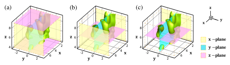
Figure 3: Case study of PINNs for incompressible flows: problem setup for 3D flow reconstruction from 2D2C observations. (a) Case 1: two x-planes ($x=1.5,7.5$), one y-plane ($y=0$) and two z-planes ($z=4.0,9.0$) are observed. (b) Case 2: two x-planes ($x=1.5,7.5$), one y-plane ($y=0$) and one z-plane ($z=6.4$) are observed. (c) Case 3: one x-plane ($x=1.5$), one y-plane ($y=0$) and one z-plane ($z=6.4$) are observed. Note that for the cross-planes, only the projected vectors are measured. The goal is to infer the 3D flow in the investigated domain using PINNs from these 2D2C observations.

3.1 Problem setup

We consider the 3D wake flow past a stationary cylinder at Reynolds number $\text{Re}=200$ in this section. In order to evaluate the performance of PINNs, we generate the reference solution numerically by using the spectral/hp element method GK_CFDbook . The computational domain is defined as $\Omega$: $[-7.5,28.5]\times[-20,20]\times[0,12.5]$, where the coordinates are non-dimensionalized by the diameter of the cylinder. The center of the cylinder is located at $(x,y)=(0,0)$. We assume that the velocity ($u=1$) is uniform at the inflow boundary where $x=-7.5$. A periodic boundary condition is used at the lateral boundaries where $y=\pm 20$, and the zero-pressure is prescribed at the outlet where $x=28.5$. Moreover, the no-slip boundary condition is imposed on the cylinder surface. The governing equations in this case study are the dimensionless incompressible Navier-Stokes equations with $\text{Re}=200$. Under this configuration, the wake flow over the cylinder is 3D and unsteady. The simulation is performed until the vortex shedding flow becomes stable. At the end, the time-dependent data are collected for PINN training and evaluation.

The simulation results of the 3D flow are shown in Fig. 2, where Fig. 2(a) shows the iso-surface of streamwise vorticity ($\omega_{x}=-0.3$) color-coded with the streamwise velocity $u$. In this section, we are interested in the 3D flow reconstruction problem from limited data, and we only focus on a sub-domain in the wake flow, namely $\Omega_{s}$: $[1.5,7.5]\times[-3,3]\times[4,9]$, which is represented by a cube with blue edges in Fig. 2(a). The contours of the three velocity components and pressure field are shown in Fig. 2(b). An Eulerian mesh with $61\times 61\times 26$ grid points is used for plotting. To demonstrate the unsteadiness of the motion, we consider 50 snapshots with $\Delta t=0.2$, which is about two periods of the vortex shedding cycle.

Here, we aim to apply PINNs for reconstructing the 3D flow field from the velocity observations of a few 2D planes. As illustrated in Fig. 3, three different “experimental” setups are considered in this paper:

• Case 1: two x-planes ($x=1.5,7.5$), one y-plane ($y=0$) and two z-planes ($z=4.0,9.0$) are observed.

• Case 2: two x-planes ($x=1.5,7.5$), one y-plane ($y=0$) and one z-plane ($z=6.4$) are observed.

• Case 3: one x-plane ($x=1.5$), one y-plane ($y=0$) and one z-plane ($z=6.4$) are observed.

We note that for these cross-planes, only the projected vectors (two components) are considered known. For example, the velocities $(u,v)$ can be observed on the z-plane, while the orthogonal component $(w)$ is unknown. The purpose of doing this is to mimic the planar particle image velocimetry in real experiments. Moreover, the resolutions of these 2D2C observations are different, which can be found in Table 1.

Table 1: Case study of PINNs for incompressible flows: details of the 2D2C observations.

Cross-section	Observed	Observed
	velocity components	spatial resolution
x-plane	$(v,w)$	$61\times 26$
y-plane	$(u,w)$	$61\times 26$
z-plane	$(u,v)$	$61\times 61$

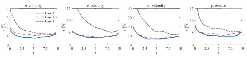
Figure 4: Case study of PINNs for incompressible flows: relative $L_{2}$-norm errors of velocities and pressure for different flow reconstruction setups. These three cases correspond to those shown in Fig. 3. The errors are computed over the entire investigated domain.

3.2 Implementation of PINNs

Given the observation data on the cross-planes, we train a PINNs model to approximate the flow fields over the space-time domain. The PINN in this section take $(\mathbf{x},t)=(x,y,z,t)$ as inputs and outputs the velocity and pressure $(u,v,w,p)$. The loss function in PINN can be defined as:

$${L}={L}_{data}+{L}_{PDE},$$ (4)

where

$${L}_{data}= \frac{1}{N_{u}}\sum_{i}^{N_{u}}\parallel u(\mathbf{x}^{i}_{data},t^{i}_{data})-u^{i}_{data}\parallel^{2}$$ (5)

$$+\frac{1}{N_{v}}\sum_{i}^{N_{v}}\parallel v(\mathbf{x}^{i}_{data},t^{i}_{data})-v^{i}_{data}\parallel^{2}$$

$$+\frac{1}{N_{w}}\sum_{i}^{N_{w}}\parallel w(\mathbf{x}^{i}_{data},t^{i}_{data})-w^{i}_{data}\parallel^{2},$$

and

$${L}_{PDE}= \frac{1}{N_{f}}\sum_{i}^{N_{f}}\sum_{j}^{4}\parallel f_{j}(\mathbf{x}^{i}_{f},t^{i}_{f})\parallel^{2},$$ (6)

$$f_{1,2,3} =\frac{\partial\mathbf{u}}{\partial t}+(\mathbf{u}\cdot\nabla)\mathbf{u}+\nabla p-\frac{1}{\text{Re}}\nabla^{2}\mathbf{u},$$

$$f_{4} =\nabla\cdot\mathbf{u}.$$

The data loss ${L}_{data}$ is composed of three components, and the number of training data (namely $N_{u}$, $N_{v}$ and $N_{w}$) depends on the number of observed planes, the data resolution of each plane as well as the number of snapshots. On the other hand, the residual points for ${L}_{PDE}$ can be randomly selected, and here we sample $N_{f}=3\times 10^{6}$ points over the investigated space and time domain $\Omega_{s}$. Note that in this study, the boundary and initial conditions are not required unlike the classical setting. Moreover, no information about the pressure is given. The weighting coefficients for the loss terms are all equal to 1.

A fully-connected neural network with 8 hidden layers and 200 neurons per layer is employed. The activation function of each neuron is $\sigma=sin(\cdot)$. We apply the ADAM optimizer with mini-batch for network training, where a batch size of $N=10^{4}$ is used for both data and residual points. The network is trained for 150 epochs with learning rates $1\times 10^{-3}$, $5\times 10^{-4}$ and $1\times 10^{-4}$ for every 50 epochs. After training, the velocity and pressure fields are evaluated on the Eulerian grid for comparison and visualization.

3.3 Inference results

For a quantitative assessment, we first define the relative $L_{2}$-norm error as the evaluation metric, which is expressed as:

$$\epsilon_{V}=\frac{\parallel V_{CFD}-\hat{V}\parallel^{2}}{\parallel V_{CFD}\parallel^{2}}\times 100\%,$$ (7)

where $V\in\{u,v,w,p\}$; $V_{CFD}$ and $\hat{V}$ account for the CFD data and the output of PINNs, respectively. We compute the errors in the investigated time domain, which are shown in Fig. 4. It can be seen from the plots that PINNs can infer the 3D flow very accurately for Case 1 and Case 2; using 5 planes (Case 1) is slightly better than using 4 planes (Case 2). When only 3 cross-planes are available (Case 3), the errors become much larger. However, the result of Case 3 is still acceptable as we are able to infer the main flow features with high accuracy (the error of the streamwise velocity is mostly less than 2%). We note that the errors of $w$-velocity are larger than the other components since the $w$-velocity magnitude is relatively small. Moreover, we observe larger discrepancy for the initial and final time instants, which can be attributed to the lack of training data for computing derivatives at $t<0$ and $t>10$. This generally happens in the cases when the initial condition is not provided in the unsteady case raissi2020hidden .

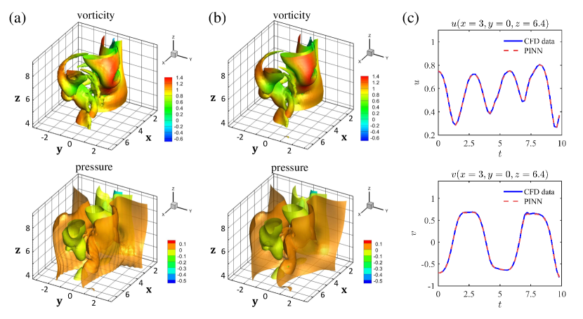
Figure 5: Case study of PINNs for incompressible flows: inference result of PINNs for Case 2. (a) Iso-surfaces of vorticity magnitude (top) and pressure (bottom) at $t=8.0$ from CFD data. (b) Iso-surfaces of vorticity magnitude (top) and pressure (bottom) at $t=8.0$ inferred by PINNs. (c) Point measurement $(x=3,y=0,z=6.4)$ of velocity $(u,v)$ against time. In this case, the 3D flow is inferred by PINNs from four cross-planes.

To visualize more details, we emphasize the result of Case 2 and demonstrate the iso-surface of vorticity magnitude and iso-surfaces of pressure at $t=8.0$ in Fig. 5, where Fig. 5(a) shows the reference CFD data and Fig. 5(b) shows the result inferred by PINNs. The vorticity value is $|\omega|=1.2$ and the color represents the streamwise velocity component. It can be seen that the PINNs inference result (inferred from a few 2D2C observations) is very consistent with the CFD simulation. In addition, the velocities $(u,v)$ at a single point $(x=3,y=0,z=6.4)$ against time are plotted in Fig. 5(c), where we can find that PINNs can capture the unsteadiness of vortex shedding flow very accurately.

4 Case Study for Compressible Flows

PINNs have also been used in simulating high-speed flows mao2020physics . In this section, we consider the following 2D steady compressible Euler equations:

$$\nabla\cdot{f}(U)=0,\;x\in\Omega\subset\mathbb{R}^{2},$$ (8)

where

$$U=[\rho,\rho u,\rho v,\rho E]^{T},\;{f}=(G_{1},G_{2})$$

with $G_{1}(U)=[\rho u,p+\rho u^{2},\rho uv,pu+\rho uE],\;G_{2}(U)=[\rho v,\rho uv,p+\rho v^{2},pv+\rho vE].$ Here, $\rho$ is the density, $p$ is the pressure, $[u,\,v]$ are the velocity components, and $E$ is the total energy. We use the additional equation of state, which describes the relation of the pressure and energy, to close the above Euler equations. For instance, we consider the equation of state for a polytropic gas given by

$$p=(\gamma-1)\left(\rho E-\frac{1}{2}\rho\|{\bm{u}}\|^{2}\right),$$ (9)

where $\gamma$ is the adiabatic index and $\bm{u}=(u,v)$.

We shall employ the PINNs to solve the inverse problem of the compressible Euler equ. 8. In particular, we shall infer the density, pressure and velocity fields by using PINNs based on the information of density gradients, limited data of pressure (pressure on the surface of the body), inflow conditions and global physical constrains.

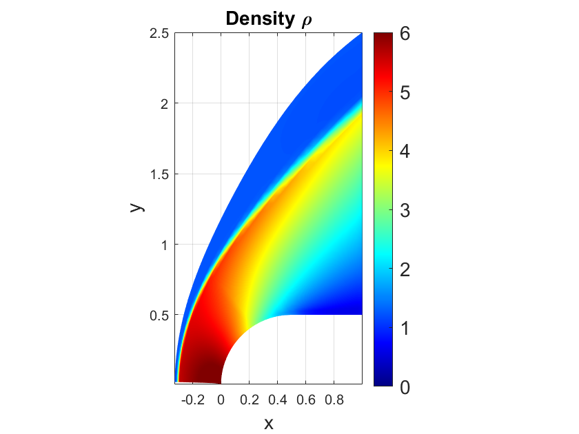
(a)

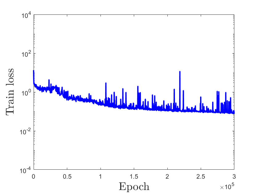
(b)

Figure 6: Case study of PINNs for compressible flows. Left: the density obtained by using CFD simulation with the inlet flow condition (11). Right: training loss vs. number of epochs.

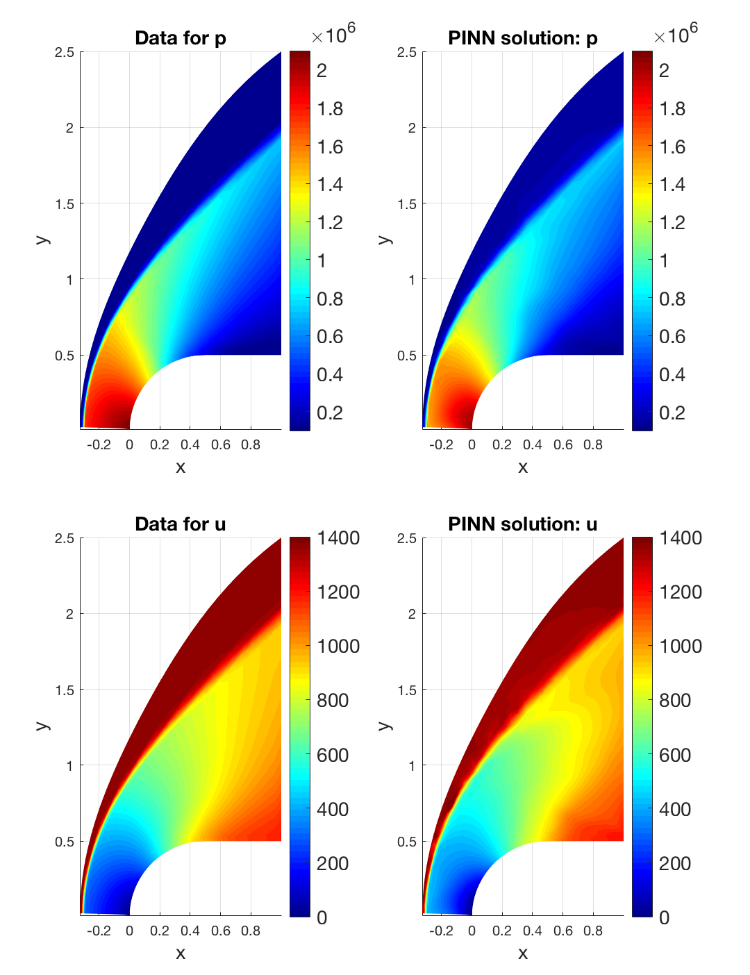
Figure 7: Case study of PINNs for compressible flows. Comparison between the PINN solutions and the CFD solutions. Top: pressure $p$, Bottom: velocity component $u$.

4.1 Problem setup

We consider a 2D bow shock wave problem. For traditional CFD simulations, it is crucial that the boundary conditions, which play an important role, are properly implemented. However, for the shock wave problem in high-speed flows, the boundary conditions in real experiments are usually not known and can only be estimated approximately. In the present work, instead of using most of the boundary conditions required by the traditional CFD simulation, we solve the Euler equ. 8 using PINNs based on the data of density gradients $\nabla\rho$ motivated by the Schlieren photography available experimentally; additionally, we use limited data of the surface pressure obtained by pressure sensors as well as the global constrains (mass, momentum and energy). We also use the inflow conditions here. Note that unlike the one-dimensional case, where the density gradient in the whole computational domain is used in mao2020physics , here we only use the density gradients in a sub-domain $D$ of the computational domain $\Omega$, i.e., $D\subset\Omega$. By combining the mathematical model and the given data, we have the weighted loss function of PINN given by

$$Loss=\omega_{1}Loss_{F}+\omega_{2}Loss_{\nabla\rho|_{D}}+\omega_{3}Loss_{inflow}+\omega_{4}Loss_{p^{*}}$$ (10)

$$+\omega_{5}\left(Loss_{Mass}+Loss_{Momentum}+Loss_{Energy}\right)+\omega_{6}Loss_{n\cdot{\bm{u}}},$$

whre the last term corresponds to the velocity condition on the surface.

4.2 Inference results

To demonstrate the effectiveness of PINNs for compressible flows, we consider the bow shock problem with the following inlet flow conditions

$$M_{\infty}=4,\;p_{\infty}=101253.6Pa,\;\rho_{\infty}=1.225kg/m^{3},$$ (11)

$$u_{\infty}=1360.6963m/s,\;v_{\infty}=0,\;T_{\infty}=288K.$$

The data points for the pressure are located on the surface of the body. By using the above inflow conditions and CFD code, we can obtain the steady state flow. We show the density computed by CFD in the left plot of Fig. 6. We employ a $6\times 60$ (6 hidden layer) neural network and train it by using layer-wise adaptive tanh activate function jagtap2020adaptive and the Adam optimizer with the learning late being $6\times 10^{-4}$ and $3\times 10^{5}$ epochs. Here, we also use the technique of dynamic weights wang2020understanding ; jin2021nsfnets . The history of the training loss is shown in the right plot of Fig. 6. The results of the PINN solutions for the pressure and velocity ($u$) are shown in Fig. 7. Observe that the PINN solutions are in good agreement with the CFD data. This indicates that we can reconstruct the flow fields for high-speed flows using some other available knowledge different from the boundary conditions required by the traditional CFD simulation.

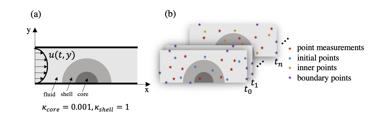
Figure 8: Case study for 2D flow past a thrombus with phase dependent permeability. (a) A channel with walls on the top and bottom boundaries with the inlet flow $u(t,y)$ entering from the left side; $\phi$=1 is the fluid. A thrombus with an impermeable core $\phi=-1$ and permeable shell $\phi=0$ is present at the bottom boundary. (b) Sampling points for inferring permeability include initial points ($\star$) at the time $t_{0}$, inner points ($\star$) from $t_{1}$ to $t_{n}$, boundary points ($\star$) on boundaries, and point measurements ($\star$) with PDE solutions. (Figure adapted from yin2021non ).

5 Case Study for Biomedical Flows

In addition to the aforementioned flow examples, PINNs have also been used in biomedical flows yin2021non . In this section, we consider inferring material properties of a thrombus in arterial flow described by the Navier-Stokes and Cahn-Hilliard equations. Such equations can be used for describing the mechanical interaction between thrombus and blood flow as a fluid-structure interaction (FSI) problem. The PDE system can be written as:

$$\rho(\frac{\partial\mathbf{u}}{\partial t}+\mathbf{u}\cdot\nabla\mathbf{u})+\nabla p =\nabla\cdot(\bm{\sigma_{vis}}+\bm{\sigma_{coh}})-\mu\frac{(1-\phi)\mathbf{u}}{2\kappa(\phi)},$$ (12)

$$\nabla\cdot\mathbf{u} =0,$$ (13)

$$\frac{\partial\bm{\psi}}{\partial t}+\mathbf{u}\cdot\nabla\bm{\psi} =0,$$ (14)

$$\frac{\partial\phi}{\partial t}+\mathbf{u}\cdot\nabla\phi =\tau\Delta\omega,$$ (15)

$$\omega =\Delta\phi+\gamma g(\phi),$$ (16)

$g(\phi)$ is the derivative of the double-well potential $(\phi^{2}-1)^{2}/4h^{2}$. $\mathbf{u}(\mathbf{x},t)$, $p(\mathbf{x},t)$ $\bm{\sigma}(\mathbf{x},t)$, and $\phi(\mathbf{x},t)$ represent the velocity, pressure, stress, and phase field. $h$ is the interfacial length; $\psi$ denotes the auxiliary vector and its gradients are the components of the deformation gradient tensor $\mathbf{F}$ as follows:

$$\mathbf{F}:=\begin{bmatrix}-\frac{\partial\psi_{1}}{\partial y}&-\frac{\psi_{2}}{\partial y}\\ \frac{\partial\psi_{1}}{\partial x}&\frac{\partial\psi_{2}}{\partial x}\end{bmatrix}.$$

Equ. 12 is the Navier-Stokes equation with viscous and cohesive stresses, respectively, which can be written as:

$$\bm{\sigma_{vis}}=\mu\nabla u,$$ (17)

$$\bm{\sigma_{coh}}=\lambda\nabla\cdot(\nabla\phi\otimes\phi).$$ (18)

Moreover, $\gamma$, $\tau$, and $\lambda$ are the interfacial mobility, relaxation parameter, and mixing energy density, respectively. We follow the normalization in wufsus2013hydraulic and write $\kappa=\frac{k_{f}}{a_{f}^{2}}$, $k_{f}$ is the true permeability and $a_{f}$ is the fibrin radius. We set the density $\rho$ = 1, viscosity $\mu$ = 0.1, $\lambda$ = $4.2428\times 10^{-5}$, $\tau$ = $10^{-6}$, and the interface length $h$= 0.05. These parameters in PINNs are non-dimensionalized values so as to be consistent with the CFD solver.

The velocity at inlet $\Gamma_{i}$ is set as Dirichlet boundary conditions $\textbf{u}=g,(\textbf{x},t)\in\Gamma_{i}\times(0,T)$. We impose the no-slip boundary on the wall $\Gamma_{w}$ and Neumann boundary conditions, i.e., $\frac{\partial\phi}{\partial\textbf{n}}=\frac{\partial\omega}{\partial\textbf{n}}=0,\textbf{x}\in\Gamma_{w}\cup\Gamma_{i}\cup\Gamma_{o}$ for $\phi$ and $\omega$ at all boundaries.

5.1 PINNs

We construct two fully-connected neural networks, Net U and Net W, where the outputs of Net U represents a surrogate model for the PDE solutions u, v, p, and $\phi$ and the outputs of Net W are PDE solutions $\omega$, $\psi_{1}$, and $\psi_{2}$. Each network has 9 hidden layers with 20 neurons per layer. The total loss L is a combination of different losses as:

$$L=\omega_{1}L_{PDE}+\omega_{2}L_{IC}+\omega_{3}L_{BC}+\omega_{4}L_{data},$$ (19)

where $L_{PDE}$ is the PDEs residual loss, $L_{IC}$ is the initial condition loss, $L_{BC}$ is the boundary condition loss, and $L_{data}$ is the data loss. In particular:

$$L_{PDE}(\theta,\bm{\lambda};X_{PDE}) =\frac{1}{\left|X_{PDE}\right|}\sum\limits_{\textbf{x}\in X_{PDE}}\left\lVert f(\textbf{x},\partial_{t}{\hat{\textbf{u}}},\partial_{x}\hat{\textbf{u}},...;\bm{\lambda})\right\rVert_{2}^{2},$$ (20)

$$L_{BC}(\theta,\bm{\lambda};X_{BC}) =\frac{1}{\left|X_{BC}\right|}\sum\limits_{\textbf{x}\in X_{BC}}\left\lVert\mathfrak{B(\hat{\textbf{u}},\textbf{x})}\right\rVert_{2}^{2},$$ (21)

$$L_{IC}(\theta,\bm{\lambda};X_{IC}) =\frac{1}{\left|X_{IC}\right|}\sum\limits_{\textbf{x}\in X_{IC}}\left\lVert\hat{\textbf{u}}-\textbf{u}_{t_{0}}\right\rVert_{2}^{2},$$ (22)

$$L_{data}(\theta,\bm{\lambda};X_{data}) =\frac{1}{|X_{data}|}\sum\limits_{\textbf{x}\in X_{data}}\left\lVert\hat{\textbf{u}}-\textbf{u}_{data}\right\rVert_{2}^{2},$$ (23)

where $\omega_{1}$, $\omega_{2}$, $\omega_{3}$, and $\omega_{4}$ are the weights of each term. The training sets $X_{PDE}$, $X_{BC}$, and $X_{IC}$ are sampled from the inner spatio-temporal domain, boundaries, and initial snapshot, respectively. $X_{data}$ is the set that contains sensor coordinates and point measurements; $\left|\cdot\right|$ denotes the number of training data in the training set. In particular, $\mathfrak{B}$ represents a combination of the Dirichlet and Neumann residuals at boundaries. Finally, we optimize the model parameters $\bm{\theta}$ and the PDE parameters $\bm{\lambda}=[\kappa]$ by minimizing the total loss $L(\bm{\theta},\bm{\lambda})$ iteratively until the loss satisfies the stopping criteria. Minimizing the total loss is an optimization process for $\bm{\lambda}$ such that the outputs of the PINN satisfy the PDE system, initial/boundary conditions, and point measurements.

5.2 Problem setup

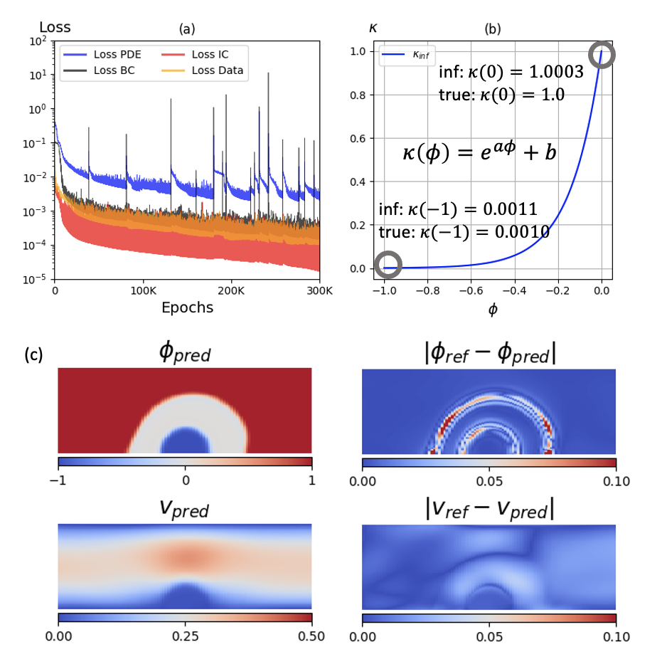
Figure 9: Inference results for 2D flow past a thrombus with phase-dependent permeability. (a) History of network losses (Loss PDE, Loss IC, Loss BC, and Loss Data) and (b) inferred permeability $\kappa$ as a function of $\phi$. (c) Comparison of phase field and velocity field for $\kappa(\phi)$ at $t$ = 0.78 and their absolute error. The core permeability is 0.001 and the shell permeability is set 1 as the actual values. 10,000 data points are scattered in the spatio-temporal domain from 30 snapshots ($t\in[0.03,0.93]$) as the training data to infer the permeability. Inferred $a$ and $b$ are 7.10 and 0.0003 compared to the true value at 6.9 and 0.0. (Figure adapted from yin2021non )

We consider a computational setup with a semi-circle permeable thrombus in a channel with a steady parabolic flow coming from the left (Fig. 8). This setup is meaningful in a sense that it presents an idealized thrombus with an impermeable core, which consists of a fibrin clot and a permeable shell (consisting of loosely-packed and partially-activated platelets). This model has been adapted as an idealized thrombus in previous works zheng2020three ; xu2008multiscale ; yazdani2017general . The goal is to infer the unknown permeability (for the shell and core) and velocity field based on the measurable phase field data. Fig. 8(b) presents all the types of training data, namely the initial snapshot $t_{0}$ ($\star$), inner spatio-temporal domain from $t_{1}$ to $t_{n}$ ($\star$), and at the boundaries ($\star$). Also, point measurements ($\star$) including their coordinates and phase field value are sampled in the spatio-temporal domain to calculate the data loss term in the total loss. We draw 1,000 points from an initial snapshot, 10,000 inner points to compute the PDE residuals, and 1,000 boundary points to compute the residuals at boundaries. Note that point measurements and inner points are drawn from the inner spatio-temporal domain; the former contains the PDE solutions whereas the latter does not.

The thrombus is present in the middle of the channel as shown in Fig. 8(a) with permeability $\kappa=0.001$ in the core ($\phi=-1$) and $\kappa=1$ in the outer shell layer ($\phi=0$). To express such spatial variation explicitly, we consider a relation between $\phi$ and $\kappa$ in this case:

$$\kappa(\phi)=e^{a\phi}+b,$$ (24)

where $a$ and $b$ are model parameters to be optimized in the PINN model and the true values of $a$ and $b$ are 6.90 and 0.0. Notice that the relation is not unique in terms of its form as long as the permeability value matches the true value for $\phi=0$ and $1$.

5.3 Inference Results

We present the inference results in Fig. 9. Fig. 9(a) shows the history of the different losses, namely PDE loss, boundary condition loss (Loss BC), initial condition loss (Loss IC), and data loss (Loss Data) in (a). We trained the model with 300,000 epochs with PDE loss as the largest component. The other errors are lower than $O(10^{-3})$ Plot (b) shows the inference result for $\kappa$ as a function of $\phi$; the inferred $a$ and $b$ are at 7.1 and 0.0003, indicating that the permeability at core area ($\kappa(\phi=-1)=0.0011$) and shell area ($\kappa(\phi=0)=1.0003$) match the reference values well. As a qualitative comparison, we present the predicted fields of $\phi_{pred}$ and $v_{pred}$ and their difference with the reference data at $t=0.78$ in Fig. 9(c). The phase field prediction exhibits a good agreement compared with the ground truth data. More importantly, the hidden velocity field can also be accurately inferred only based on the phase field data. Notice that the errors for the phase field are mainly distributed in and around the outlet layer of the thrombus and the errors in velocity field are mainly confined within the shell layer.

6 Summary

PINNs offer a new approach to simulating realistic fluid flows, where some data are available from multimodality measurements whereas the boundary conditions or initial conditions may be unknown. While this is perhaps the prevailing scenario in practice, existing CFD solvers cannot handle such ill-posed problems and hence one can think of PINNs for fluid problems as a complementary approach to the plethora of existing numerical methods for CFD for idealized problems.

There are several opportunities for further research, e.g., using PINNs for active flow control to replace expensive experiments and time-consuming large-scale simulations as in fan2020reinforcement , or predict fast the flow at a new high Reynolds number using transfer learning techniques assuming we have available solutions at lower Reynolds numbers. Moreover, a new area for exploration could be the development of closure models for unresolved flow dynamics at very high Reynolds number using the automatic data assimilation method provided by PINNs. Computing flow problems at scale requires efficient multi-GPU implementations in the spirit of data parallel hennigh2020nvidia or a hybrid data parallel and model parallel paradigms as in shukla2021parallel . The parallel speed up obtained for flow simulations so far is very good, suggesting that PINNs can be used in the near future for industrial complexity problems at scale that CFD methods cannot tackle.

- (1) Brooks, A.N., Hughes, T.J.: Streamline upwind/Petrov-Galerkin formulations for convection dominated flows with particular emphasis on the incompressible Navier-Stokes equations. Computer Methods in Applied Mechanics and Engineering 32(1-3), 199–259 (1982)
- (2) Karniadakis, G.E., Sherwin, S.: Spectral/hp Element Methods for Computational Fluid Dynamics, 2nd edition. Oxford University Press, Oxford,UK (2005)
- (3) Katz, A.J.: Meshless methods for computational fluid dynamics. Stanford University Stanford, CA (2009)
- (4) Liu, M., Liu, G.: Smoothed particle hydrodynamics (SPH): an overview and recent developments. Archives of Computational Methods in Engineering 17(1), 25–76 (2010)
- (5) Beck, J.V., Blackwell, B., Clair Jr, C.R.S.: Inverse heat conduction: Ill-posed problems. James Beck (1985)
- (6) Jasak, H., Jemcov, A., Tukovic, Z., et al.: OpenFOAM: A C++ library for complex physics simulations. In: International Workshop on Coupled Methods in Numerical Dynamics, vol. 1000, pp. 1–20. IUC Dubrovnik Croatia (2007)
- (7) Raissi, M., Perdikaris, P., Karniadakis, G.E.: Physics informed learning machine (2021). US Patent 10,963,540
- (8) Raissi, M., Perdikaris, P., Karniadakis, G.E.: Machine learning of linear differential equations using Gaussian processes. Journal of Computational Physics 348, 683–693 (2017)
- (9) Raissi, M., Perdikaris, P., Karniadakis, G.E.: Numerical Gaussian processes for time-dependent and nonlinear partial differential equations. SIAM Journal on Scientific Computing 40(1), A172–A198 (2018)
- (10) Raissi, M., Wang, Z., Triantafyllou, M.S., Karniadakis, G.E.: Deep learning of vortex-induced vibrations. Journal of Fluid Mechanics 861, 119–137 (2019)
- (11) Jin, X., Cai, S., Li, H., Karniadakis, G.E.: NSFnets (Navier-Stokes flow nets): Physics-informed neural networks for the incompressible Navier-Stokes equations. Journal of Computational Physics 426, 109951 (2021)
- (12) Raissi, M., Yazdani, A., Karniadakis, G.E.: Hidden fluid mechanics: Learning velocity and pressure fields from flow visualizations. Science 367(6481), 1026–1030 (2020)
- (13) Mao, Z., Jagtap, A.D., Karniadakis, G.E.: Physics-informed neural networks for high-speed flows. Computer Methods in Applied Mechanics and Engineering 360, 112789 (2020)
- (14) Yin, M., Zheng, X., Humphrey, J.D., Karniadakis, G.E.: Non-invasive inference of thrombus material properties with physics-informed neural networks. Computer Methods in Applied Mechanics and Engineering 375, 113603 (2021)
- (15) Raissi, M., Perdikaris, P., Karniadakis, G.E.: Physics-informed neural networks: A deep learning framework for solving forward and inverse problems involving nonlinear partial differential equations. Journal of Computational Physics 378, 686–707 (2019)
- (16) Kingma, D.P., Ba, J.: Adam: A method for stochastic optimization. arXiv preprint arXiv:1412.6980 (2014)
- (17) Abadi, M., Barham, P., Chen, J., Chen, Z., Davis, A., Dean, J., Devin, M., Ghemawat, S., Irving, G., Isard, M., et al.: Tensorflow: A system for large-scale machine learning. In: 12th USENIX symposium on operating systems design and implementation (OSDI 16), pp. 265–283 (2016)
- (18) Paszke, A., Gross, S., Massa, F., Lerer, A., Bradbury, J., Chanan, G., Killeen, T., Lin, Z., Gimelshein, N., Antiga, L., et al.: Pytorch: An imperative style, high-performance deep learning library. arXiv preprint arXiv:1912.01703 (2019)
- (19) Raissi, M., Perdikaris, P., Karniadakis, G.E.: Physics informed deep learning (part i): Data-driven solutions of nonlinear partial differential equations. arXiv preprint arXiv:1711.10561 (2017)
- (20) Raissi, M., Perdikaris, P., Karniadakis, G.E.: Physics informed deep learning (part ii): Data-driven discovery of nonlinear partial differential equations. arxiv. arXiv preprint arXiv:1711.10561 (2017)
- (21) Pang, G., Lu, L., Karniadakis, G.E.: fPINNs: Fractional physics-informed neural networks. SIAM Journal on Scientific Computing 41(4), A2603–A2626 (2019)
- (22) Fang, Z., Zhan, J.: A physics-informed neural network framework for PDEs on 3D surfaces: Time independent problems. IEEE Access 8, 26328–26335 (2019)
- (23) Zhang, D., Guo, L., Karniadakis, G.E.: Learning in modal space: Solving time-dependent stochastic PDEs using physics-informed neural networks. SIAM Journal on Scientific Computing 42(2), A639–A665 (2020)
- (24) Kharazmi, E., Zhang, Z., Karniadakis, G.E.: hp-VPINNs: Variational physics-informed neural networks with domain decomposition. Computer Methods in Applied Mechanics and Engineering 374, 113547 (2021)
- (25) Jagtap, A.D., Kharazmi, E., Karniadakis, G.E.: Conservative physics-informed neural networks on discrete domains for conservation laws: Applications to forward and inverse problems. Computer Methods in Applied Mechanics and Engineering 365, 113028 (2020)
- (26) Jagtap, A.D., Karniadakis, G.E.: Extended Physics-Informed Neural Networks (XPINNs): A generalized space-time domain decomposition based deep learning framework for nonlinear partial differential equations. Communications in Computational Physics 28(5), 2002–2041 (2020)
- (27) Shukla, K., Jagtap, A.D., Karniadakis, G.E.: Parallel physics-informed neural networks via domain decomposition. arXiv preprint arXiv:2104.10013 (2021)
- (28) Hennigh, O., Narasimhan, S., Nabian, M.A., Subramaniam, A., Tangsali, K., Rietmann, M., Ferrandis, J.d.A., Byeon, W., Fang, Z., Choudhry, S.: NVIDIA SimNet^TM: an AI-accelerated multi-physics simulation framework. arXiv preprint arXiv:2012.07938 (2020)
- (29) Yang, Y., Perdikaris, P.: Adversarial uncertainty quantification in physics-informed neural networks. Journal of Computational Physics 394, 136–152 (2019)
- (30) Zhang, D., Lu, L., Guo, L., Karniadakis, G.E.: Quantifying total uncertainty in physics-informed neural networks for solving forward and inverse stochastic problems. Journal of Computational Physics 397, 108850 (2019)
- (31) Zhu, Y., Zabaras, N., Koutsourelakis, P.S., Perdikaris, P.: Physics-constrained deep learning for high-dimensional surrogate modeling and uncertainty quantification without labeled data. Journal of Computational Physics 394, 56–81 (2019)
- (32) Sun, L., Wang, J.X.: Physics-constrained Bayesian neural network for fluid flow reconstruction with sparse and noisy data. Theoretical and Applied Mechanics Letters 10(3), 161–169 (2020)
- (33) Yang, L., Meng, X., Karniadakis, G.E.: B-PINNs: Bayesian physics-informed neural networks for forward and inverse PDE problems with noisy data. Journal of Computational Physics 425, 109913 (2021)
- (34) Meng, X., Karniadakis, G.E.: A composite neural network that learns from multi-fidelity data: Application to function approximation and inverse PDE problems. Journal of Computational Physics 401, 109020 (2020)
- (35) Jagtap, A.D., Kawaguchi, K., Karniadakis, G.E.: Adaptive activation functions accelerate convergence in deep and physics-informed neural networks. Journal of Computational Physics 404, 109136 (2020)
- (36) Wang, S., Teng, Y., Perdikaris, P.: Understanding and mitigating gradient pathologies in physics-informed neural networks. arXiv preprint arXiv:2001.04536 (2020)
- (37) Lu, L., Pestourie, R., Yao, W., Wang, Z., Verdugo, F., Johnson, S.G.: Physics-informed neural networks with hard constraints for inverse design. arXiv preprint arXiv:2102.04626 (2021)
- (38) Gao, H., Sun, L., Wang, J.X.: PhyGeoNet: physics-informed geometry-adaptive convolutional neural networks for solving parameterized steady-state PDEs on irregular domain. Journal of Computational Physics 428, 110079 (2021)
- (39) Shin, Y., Darbon, J., Karniadakis, G.E.: On the convergence of physics informed neural networks for linear second-order elliptic and parabolic type PDEs. Communications in Computational Physics 28, 2042–2074 (2020)
- (40) Mishra, S., Molinaro, R.: Estimates on the generalization error of physics informed neural networks (PINNs) for approximating PDEs. arXiv preprint arXiv:2006.16144 (2020)
- (41) Wang, S., Yu, X., Perdikaris, P.: When and why PINNs fail to train: A neural tangent kernel perspective. arXiv preprint arXiv:2007.14527 (2020)
- (42) Kissas, G., Yang, Y., Hwuang, E., Witschey, W.R., Detre, J.A., Perdikaris, P.: Machine learning in cardiovascular flows modeling: Predicting arterial blood pressure from non-invasive 4D flow MRI data using physics-informed neural networks. Computer Methods in Applied Mechanics and Engineering 358, 112623 (2020)
- (43) Yang, X., Zafar, S., Wang, J.X., Xiao, H.: Predictive large-eddy-simulation wall modeling via physics-informed neural networks. Physical Review Fluids 4(3), 034602 (2019)
- (44) Lou, Q., Meng, X., Karniadakis, G.E.: Physics-informed neural networks for solving forward and inverse flow problems via the Boltzmann-BGK formulation. arXiv preprint arXiv:2010.09147 (2020)
- (45) Cai, S., Wang, Z., Wang, S., Perdikaris, P., Karniadakis, G.E.: Physics-informed neural networks for heat transfer problems. Journal of Heat Transfer 143(6), 060801 (2021)
- (46) Cai, S., Wang, Z., Fuest, F., Jeon, Y.J., Gray, C., Karniadakis, G.E.: Flow over an espresso cup: inferring 3-D velocity and pressure fields from tomographic background oriented Schlieren via physics-informed neural networks. Journal of Fluid Mechanics 915 (2021)
- (47) Wang, S., Perdikaris, P.: Deep learning of free boundary and stefan problems. Journal of Computational Physics 428, 109914 (2021)
- (48) Lucor, D., Agrawal, A., Sergent, A.: Physics-aware deep neural networks for surrogate modeling of turbulent natural convection. arXiv preprint arXiv:2103.03565 (2021)
- (49) Mahmoudabadbozchelou, M., Caggioni, M., Shahsavari, S., Hartt, W.H., Karniadakis, G.E., Jamali, S.: Data-driven physics-informed constitutive metamodeling of complex fluids: A multifidelity neural network (mfnn) framework. Journal of Rheology 65(2), 179–198 (2021)
- (50) Arzani, A., Wang, J.X., D’Souza, R.M.: Uncovering near-wall blood flow from sparse data with physics-informed neural networks. arXiv preprint arXiv:2104.08249 (2021)
- (51) Cai, S., Li, H., Zheng, F., Kong, F., Dao, M., Karniadakis, G.E., Suresh, S.: Artificial intelligence velocimetry and microaneurysm-on-a-chip for three-dimensional analysis of blood flow in physiology and disease. Proceedings of the National Academy of Sciences 118(13) (2021)
- (52) Wang, R., Kashinath, K., Mustafa, M., Albert, A., Yu, R.: Towards physics-informed deep learning for turbulent flow prediction. In: Proceedings of the 26th ACM SIGKDD International Conference on Knowledge Discovery & Data Mining, pp. 1457–1466 (2020)
- (53) Goswami, S., Anitescu, C., Chakraborty, S., Rabczuk, T.: Transfer learning enhanced physics informed neural network for phase-field modeling of fracture. Theoretical and Applied Fracture Mechanics 106, 102447 (2020)
- (54) Zhang, E., Yin, M., Karniadakis, G.E.: Physics-informed neural networks for nonhomogeneous material identification in elasticity imaging. arXiv preprint arXiv:2009.04525 (2020)
- (55) Wufsus, A., Macera, N., Neeves, K.: The hydraulic permeability of blood clots as a function of fibrin and platelet density. Biophysical journal 104(8), 1812–1823 (2013)
- (56) Zheng, X., Yazdani, A., Li, H., Humphrey, J.D., Karniadakis, G.E.: A three-dimensional phase-field model for multiscale modeling of thrombus biomechanics in blood vessels. PLOS Computational Biology 16(4), e1007709 (2020)
- (57) Xu, Z., Chen, N., Kamocka, M.M., Rosen, E.D., Alber, M.: A multiscale model of thrombus development. Journal of the Royal Society Interface 5(24), 705–722 (2008)
- (58) Yazdani, A., Li, H., Humphrey, J.D., Karniadakis, G.E.: A general shear-dependent model for thrombus formation. PLoS Computational Biology 13(1), e1005291 (2017)
- (59) Fan, D., Yang, L., Wang, Z., Triantafyllou, M.S., Karniadakis, G.E.: Reinforcement learning for bluff body active flow control in experiments and simulations. Proceedings of the National Academy of Sciences 117(42), 26091–26098 (2020)