MagneticTB: A package for tight-binding model of magnetic and non-magnetic materials

Abstract

We present a Mathematica program package MagneticTB, which can generate the tight-binding model for arbitrary magnetic space group. The only input parameters in MagneticTB are the (magnetic) space group number and the orbital information in each Wyckoff positions. Some useful functions including getting the matrix expression for symmetry operators, manipulating the energy band structure by parameters and interfacing with other software are also developed. MagneticTB can help to investigate the physical properties in both magnetic and non-magnetic system, especially for topological properties.

Program summary

Program title: MagneticTB

Licensing provisions: GNU General Public Licence 3.0

Programming language: Mathematica

External routines/libraries used: ISOTROPY (iso.byu.edu)

Developer’s repository link: https://github.com/zhangzeyingvv/MagneticTB

Nature of problem: Construct the symmetry adopted tight-binding model for the system with arbitrary magnetic space group.

1 Introduction

Tight-binding method is a powerful tool to investigate the novel properties in condensed mater physics [1, 2, 3, 4, 5]. Compared with first-principles method, tight-binding method can greatly simplify calculations. Moreover, after considering (magnetic) space group symmetry, the tight-binding model can give more reliable results. For example, in topological materials, symmetry plays an important role to protect the topological properties, such as $Z_{2}$ topological insulator protected by time reversal symmetry [6], topological crystalline insulators and topological nodal semimetals protected by space group symmetries [7, 8] and magnetic topological crystalline insulator protected by magnetic space group symmetries, i.e. the combination of space group operations and time reversal [9, 10].

At present, a lot of researchers using symmetry adopted tight-binding model to investigate physical properties of electronic system [11, 12, 13, 14, 15, 16, 17, 18, 19, 20, 21]. However, most of the software packages are mainly focused on the tight-binding model for non-magnetic materials [22, 23, 24, 25, 26] and only a few of them can be used to construct the symmetry adopted tight-binding model automatically. For the first-principles level, Wannier90 can generate the Wannier-tight-binding model by interfacing with first-principles software, but the symmetry adopted Wannier function can not be applied to other first-principles software (such as VASP, ABINIT) except Quantum-Espresso [27, 28, 29, 30]. FPLO can generate symmetry adopted tight-binding model with proper parameters for given structures [31]. Meanwhile, both Wannier90 and FPLO do not support magnetic symmetry. For the model level, GTPack, Qsymm and MathemaTB can generate the tight-binding model with space group symmetry but does not support magnetic symmetry directly [32, 33, 34]. WannierTools can do the symmetrization of non-magnetic tight-binding model but cannot generate the tight-binding model by itself [35].

Therefore, it is necessary to develop a package which can construct the tight-binding model with magnetic space group symmetry automatically. Here we introduce a software package: MagneticTB, a tool for generating the tight-binding model for the system with arbitrary magnetic space group. The required input information of this package is only the magnetic space group number and the orbital information in each Wyckoff positions. It can help to investigate the physical properties of the given symmetry. We also present some useful functions including get the matrix expression for symmetry operators, manipulate the band structure by parameters and interface with other software.

This paper is organized as follows. In Sec. 2, we give an introduction of symmetry adopted tight-binding methods. In Sec. 3, The usage of MagneticTB are given, including how to install and run MagneticTB. In Sec. 4, we give three concrete examples, such examples show the specific capabilities of the MagneticTB. Finally, conclusions are given.

2 Symmetry adopted tight-binding method

In periodic system, the bases of tight-binding model can be written as Bloch sum [11]

$$\psi_{lm\bm{k}}^{n}(\bm{r})=\frac{1}{\sqrt{N}}\sum_{\bm{R}_{j}}e^{i\bm{k}\cdot(\bm{R}_{j}+\bm{d}_{l}^{n})}\varphi_{m}^{n}(\bm{r}-\bm{R}_{j}-\bm{d}_{l}^{n})$$ (1)

where $N$ is the number of unit cells in the crystal, $\bm{R}_{j}$ is the translation vector of the Bravais lattice, $\bm{d}_{l}^{n}$ is the position of $n$-th Wyckoff position’s $l$-th atom in the unit cell (for each $Q$ and $\bm{d}_{l}^{n}$ there exists one and only one pair of $\bm{d}_{l^{\prime}}^{n}$ and $R^{\prime}$ which satisfies $Q\bm{d}_{l}^{n}=\bm{d}_{l^{\prime}}^{n}+R^{\prime}$ where $Q$ is arbitrary group element in the (magnetic) space group and $R^{\prime}$ is a lattice vector), $\varphi_{m}^{n}(\bm{r})$ is the $m$-th atomic orbital basis for position $\bm{d}_{l}^{n}$ but located at coordinate origin. Then Eq. (1) satisfies the Bloch theorem $\psi_{lm\bm{k}}^{n}(\bm{r}+\bm{R}_{j})=e^{i\bm{k}\cdot\bm{R}_{j}}\psi_{lm\bm{k}}^{n}(\bm{r})$. The tight-binding Hamiltonian can be written as:

$$\begin{split}H_{lml^{\prime}m^{\prime}}^{nn^{\prime}}(\bm{k})=&\sum_{\bm{R}_{j}}e^{i\bm{k}\cdot(\bm{R}_{j}+\bm{d}_{l^{\prime}}^{n^{\prime}}-\bm{d}_{l}^{n})}E_{mm^{\prime}}(\bm{d}_{l}^{n},\bm{R}_{j}+\bm{d}_{l^{\prime}}^{n^{\prime}})\\ E_{mm^{\prime}}(\bm{d}_{j}^{n},\bm{R}_{j}+\bm{d}_{l^{\prime}}^{n^{\prime}})=&\braket{\varphi_{m}^{n}(\bm{r}-\bm{d}_{l}^{n})}{\hat{H}}{\varphi_{m^{\prime}}^{n^{\prime}}(\bm{r}-\bm{d}_{l^{\prime}}^{n^{\prime}}-\bm{R}_{j})}\end{split}$$ (2)

for simplicity, we rewrite the atomic orbitals in vector form: $\varPhi^{n}(\bm{r}-\bm{R}_{j}-\bm{d}_{l}^{n})=\{\varphi_{m}^{n}(\bm{r}-\bm{R}_{j}-\bm{d}_{l}^{n})\},(m=1,...,M_{n})$. Then $E_{mm^{\prime}}(\bm{d}_{j},\bm{R}_{j}+\bm{d}_{l^{\prime}})$ $(m=1,...,M_{n};\,m^{\prime}=1,\dots,M_{n^{\prime}})$ form an $M_{n}\times M_{n^{\prime}}$ matrix:

$$E(\bm{d}_{l}^{n},\bm{R}_{j}+\bm{d}_{l^{\prime}}^{n^{\prime}})=\braket{\varPhi^{n}(\bm{r}-\bm{d}_{l}^{n})}{\hat{H}}{\varPhi^{n^{\prime}}(\bm{r}-\bm{R}_{j}-\bm{d}_{l^{\prime}}^{n^{\prime}})}$$ (3)

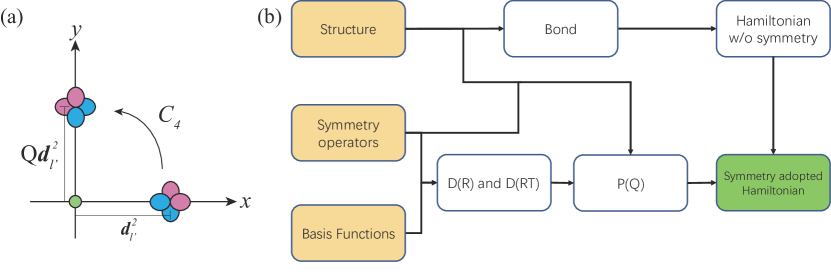
Figure 1: (a) Sketch of relationship between $E(\bm{d}_{j}^{n},\bm{R}_{j}+\bm{d}_{l^{\prime}}^{n^{\prime}})$ and $E(Q\bm{d}_{j}^{n},Q(\bm{R}_{j}+\bm{d}_{l^{\prime}}^{n^{\prime}}))$, in this example we set $Q=C_{4}{\cal T}$, $\varPhi^{1}(\bm{r})=\{s\}$ locate at $\bm{d}_{l}^{1}=(0,0)$, $\varPhi^{2}(\bm{r})=\{p_{x},p_{y}\}$ locate at $\bm{d}_{l^{\prime}}^{2}=(\lambda,0)(\lambda\neq 0)$. Then we have $D^{1}(C_{4}{\cal T})=1,D^{2}(C_{4}{\cal T})=-i\sigma_{y}$, and $E(Q\bm{d}_{l}^{1},Q\bm{d}_{l^{\prime}}^{2})=E^{*}(\bm{d}_{l}^{1},\bm{d}_{l^{\prime}}^{2})\times(-i\sigma_{y})$. (b) Workflow of MagneticTB.

Then the Hamiltonian can be rewritten as:

$$H_{ll^{\prime}}^{nn^{\prime}}(\bm{k})=\sum_{\bm{R}_{j}}e^{i\bm{k}\cdot(\bm{R}_{j}+\bm{d}_{l^{\prime}}^{n^{\prime}}-\bm{d}_{l}^{n})}E(\bm{d}_{l}^{n},\bm{R}_{j}+\bm{d}_{l^{\prime}}^{n^{\prime}})$$ (4)

$E(\bm{d}_{l}^{n},\bm{R}_{j}+\bm{d}_{l^{\prime}}^{n^{\prime}})$ is the hopping matrix between $n$-th Wyckoff position’s $l$-th atom to $n^{\prime}$-th Wyckoff position’s $l^{\prime}$-th atom. When the lattice is in invariant under some symmetry $E(\bm{d}_{l}^{n},\bm{R}_{j}+\bm{d}_{l^{\prime}}^{n^{\prime}})$ may ne not independent for arbitrary $\bm{d}_{l}^{n}$ and $\bm{d}_{l^{\prime}}^{n^{\prime}}$. Fortunately, for symmetry operation $Q$, group representation theory gives us explicit expression for the relationship between $E(Q\bm{d}_{j}^{n},Q(\bm{R}_{j}+\bm{d}_{l^{\prime}}^{n^{\prime}}))$ and $E(\bm{d}_{j}^{n},\bm{R}_{j}+\bm{d}_{l^{\prime}}^{n^{\prime}})$.

For the case that symmetry operation does not contain the time reversal ${\cal T}$, i.e. $Q=\{R|\bm{t}\}$, where $R$ and $\bm{t}$ are the rotation and translation part of $Q$ respectively, we have

$$E(Q\bm{d}_{l}^{n},Q(\bm{R}_{j}+\bm{d}_{l^{\prime}}^{n}))=D^{n}(R)E(\bm{d}_{l}^{n},\bm{R}_{l}+\bm{d}_{l^{\prime}}^{n^{\prime}})D^{n^{\prime}\dagger}(R)$$ (5)

For the case that operation $Q$ contains time reversal symmetry ${\cal T}$, i.e. $Q=\{R|\bm{t}\}{\cal T}$, we have

$$E(Q\bm{d}_{l}^{n},Q(\bm{R}_{j}+\bm{d}_{l^{\prime}}^{n}))=D^{n}(R{\cal T})E^{*}(\bm{d}_{l}^{n},\bm{R}_{j}+\bm{d}_{l^{\prime}}^{n^{\prime}})D^{n^{\prime}\dagger}(R{\cal T})$$ (6)

Where $D^{n}(R)(D^{n}(R{\cal T}))$ are the $M_{n}\times M_{n}$ representation matrices of $R(R{\cal T})$ under atomic orbital bases $\varPhi^{n}(\bm{r})$ (not necessarily irreducible representations), $E^{*}(\bm{d}_{l}^{n},\bm{R}_{j}+\bm{d}_{l^{\prime}}^{n^{\prime}})$ is complex conjugate of $E(\bm{d}_{l}^{n},\bm{R}_{j}+\bm{d}_{l^{\prime}}^{n^{\prime}})$ (see Fig. 1 for example). It is clear that for spinless cases with time reversal symmetry ${\cal T}$, when the basis functions are real, $D({\cal T})$ is equal to identity matrix, indicating that $E(\bm{d}_{l}^{n},\bm{R}_{j}+\bm{d}_{l^{\prime}}^{n^{\prime}})$ are real matrices.

The next step is to get the analytical expressions of $D^{n}(R)(D^{n}(RA))$. For a fixed $n$, we don’t have to worry about mixing superscripts of $n$ in $D^{n}(R)$ because transformations can only occur under the same $n$. So we temporarily use $D(R)$ rather than $D^{n}(R)$ in this step. Consider the following four cases:

1. Spinless system and $Q$ does not contain ${\cal T}$.

2. Spinless system and $Q$ contain ${\cal T}$.

3. Spinful system and $Q$ does not contain ${\cal T}$.

4. Spinful system and $Q$ contain ${\cal T}$.

In case. i, $D(R)$ can be obtained simply by solve the linear equation [36]

$$\hat{R}\varPhi(\bm{r})=\varPhi(R^{-1}\bm{r})=\varPhi(\bm{r})D(R)$$ (7)

in which $\hat{R}$ is the function operator for the rotation $R$. In case. ii, we define $\overline{\varPhi}(\bm{r})=\hat{{\cal T}}\varPhi(\bm{r})$, for spinless system ${\cal T}={\cal K}$, hence, $\overline{\varPhi}(\bm{r})=\varPhi^{*}(\bm{r})$ and then solve the linear equation

$$\hat{R}\hat{{\cal T}}\varPhi(\bm{r})=\overline{\varPhi}(R^{-1}\bm{r})=\varPhi(\bm{r})D(R{\cal T})$$ (8)

In case. iii, since the spin matrix is orbital independent we define the basis function as

$$\varPhi^{s}(\bm{r})={\{\varPhi(\bm{r})\uparrow,\varPhi(\bm{r})\downarrow\}}$$ (9)

The two spinors $\uparrow=(1,0)^{T}$, and $\downarrow=(0,1)^{T}$,and under the rotation $\hat{R}$ they are transformed according to

$$\hat{R}(\uparrow,\downarrow)=(\uparrow,\downarrow)D^{\frac{1}{2}}(R)$$ (10)

For proper rotation $R$, $D^{\frac{1}{2}}(R)=\text{exp}(-\frac{1}{2}i\alpha\bm{n}\cdot\hat{\bm{\sigma}})$, where $\alpha$ is the rotation angle of $R$, $\bm{n}$ is the unit vector along rotation axis, for improper rotation $S$, $R=IS$, $I$ is the inversion symmetry, $D^{\frac{1}{2}}(S)=D^{\frac{1}{2}}(R)$ [37, 38]. Then $D(R)$ can be obtained by solving the linear equation

$$\hat{R}\varPhi^{s}(\bm{r})=\varPhi^{s}(\bm{r})D(R)$$ (11)

Case. (iv) is similar to case. (ii), the only difference is replace the time reversal operator ${\cal T}={\cal K}$ by ${\cal T}=i\hat{\sigma}_{y}{\cal K}$ and consider the spin rotation matrices. The above four cases cover all the possibilities of $D(R)$ and $D(R{\cal T})$.

Then the operator (or representation matrix) for $Q$ can be defined as

$$P_{ll^{\prime}}^{nn^{\prime}}(Q)=\begin{cases}\delta_{nn^{\prime}}\tilde{\delta}_{\bm{d}_{l}^{n},Q\bm{d}_{l^{\prime}}^{n^{\prime}}}D^{n}(R)&\text{ Q does not contain ${\cal T}$}\\ \delta_{nn^{\prime}}\tilde{\delta}_{\bm{d}_{l}^{n},Q\bm{d}_{l^{\prime}}^{n^{\prime}}}D^{n}(R{\cal T})&\text{ Q contains ${\cal T}$}\end{cases}$$ (12)

where$\tilde{\delta}_{\bm{d}_{l}^{n},Q\bm{d}_{l^{\prime}}^{n^{\prime}}}$ is equal to 1 only when $d_{l}^{n}$ and $Qd_{l^{\prime}}^{n^{\prime}}$ differ by a lattice vector and to 0 otherwise (it can also be written as $\tilde{\delta}_{\bm{d}_{l}^{n},Q\bm{d}_{l^{\prime}}^{n^{\prime}}}=\delta_{\bm{d}_{l}^{n},Q\bm{d}_{l^{\prime}}^{n^{\prime}}+\bm{R}_{s}}$ if a suitable lattice vector $\bm{R}_{s}$ is choosen). The Hamiltonian under constraint of $Q$ can be written as

$$P(Q)^{-1}H(\bm{k})P(Q)=H(R^{-1}\bm{k})$$ (13)

for $Q=\{R|\bm{t}\}$, and

$$P(Q)^{-1}H(\bm{k})P(Q)=H^{*}(-R^{-1}\bm{k})$$ (14)

for $Q=\{R|\bm{t}\}{\cal T}$ [See  A for proof of Eqs.(5–6) and Eqs.(13–14)). Eqs.(13–14) are key point to generate the symmetry adopted tight-binding model. In MagneticTB we first generate the Hamiltonian with only translation symmetry and then use Eqs.(13–14) to the simplify the Hamiltonian (see Fig. 1(b)) for the workflow of MagneticTB]. The database for tight-binding model of 1651 magnetic space group can be found in our later work [39].

3 Capabilities of MagneticTB

3.1 Installation

To install the MagneticTB, unzip the "MagneticTB.zip" file and copy the MagneticTB directory to any of the following four paths:

• FileNameJoin[{$UserBaseDirectory, "Applications"}]

• FileNameJoin[{$BaseDirectory, "Applications"}]

• FileNameJoin[{$InstallationDirectory, "AddOns", "Packages"}]

• FileNameJoin[{$InstallationDirectory, "AddOns", "Applications"}]

Then one can use the package after running Needs["MagneticTB‘"]. The version of Mathematica should higher or equal to 11.0.

3.2 Running

3.2.1 Core module

To initialize the program one should identify the magnetic space group and the orbital information in each Wyckoff positions. Here we provide a function msgop to show the symmetry information of an arbitrary magnetic space group. The only input of the msgop is the magnetic space group number, one can get the symmetry information by the following code:

⬇

msgop[gray[191]]

msgop[bnsdict[{191, 236}]]

msgop[ogdict[{191, 8, 1470}]]

Magnetic space group (BNS): {191.236,P6’/mm’m}

Primitive Lattice vactor: {{a,0,0},{-a/2,(Sqrt[3] a)/2,0},{0,0,c}}

Conventional Lattice vactor: {{a,0,0},{-a/2,(Sqrt[3] a)/2,0},{0,0,c}}

{{"1",{{1,0,0},{0,1,0},{0,0,1}},{0,0,0},F},

{"3z",{{0,-1,0},{1,-1,0},{0,0,1}},{0,0,0},F},

{"3z-1",{{-1,1,0},{-1,0,0},{0,0,1}},{0,0,0},F},

{"2x",{{1,-1,0},{0,-1,0},{0,0,-1}},{0,0,0},F},

…

here gray[191] return the magnetic space group code of gray space group 191, bnsdict[{191,236}] return the magnetic space group code of BNS No. 191.236, ogdict[{191,8,1470}] return the magnetic space group code of OG No. 191.8.1470. Then the msgop will print the standard lattice vector and the symmetry operations (for primitive cell) of the corresponding magnetic space group, which can be the input of the init function. Notice the magnetic space group code is build-in constant in MagneticTB, users should use gray, bnsdict, ogdict functions rather than inputting the magnetic space group code directly.

Then one can feed the above information to init function then the basic results of input structure can be generated. The init function have five mandatory options neamly, lattice, lattpar, wyckoffposition, symminformation and basisFunctions (in ordinary Wolfram language the options for functions are optional, but such five options must be specified in MagneticTB in order to make the input clear). The lattice is the lattice vector of magnetic system which can contain parameters, lattpar is the parameters in lattice vector to determine the bond length of magnetic system,and wyckoffposition is a list to designate atomic position and magnetization-direction for each Wyckoff positions in the magnetic system. The format of wyckoffposition is:

$$\{\{\bm{a}_{1},\bm{m}_{1}\},\{\bm{a}_{2},\bm{m}_{2}\},...\}$$

where $\bm{a}_{i}$ and $\bm{m}_{i}$ represent one of the atomic positions and its magnetization-directions of the $i$-th Wyckoff position, respectively. The symminformation contain the elements of the coset of magnetic space group with respect to translation group, which can direct use the output of msgop (notice that the output of msgop is standard symmetry operation from ISOTROPY [40, 41]. However, users can also use the non-standard structure as input, not limit to the output of msgop). The format of symminformation is:

$$\{\{n_{1},R_{1},t_{1},A_{1}\},\{n_{2},R_{2},t_{2},A_{2}\},...\}$$

where $n_{i}$ is the name of symmetry operation, $R_{i}$ and $t_{i}$ are the rotation and translation part of symmetry operation, and $A_{i}$ represents whether the symmetry operation is combined with time reversal symmetry ("T" for true and "F" for false). Finally, the basisFunctions is the basis function for each Wyckoff position, The format of basisFunctions is:

$$\{b_{1},b_{2},...\}$$

where $b_{i}$ is the list of basis functions of the $i$-th Wyckoff position. The build-in basis functions for spinless case in MagneticTB is shown in Table 1.

Table 1: String codes representing basis functions and available values for basisFunctions

Basis function	String	Basis function	String
$s$	"s"	$p_{x}$	"px"
$p_{y}$	"py"	$p_{z}$	"pz"
$p_{x}+ip_{y}$	"px+ipy"	$p_{x}-ip_{y}$	"px-ipy"
$d_{z^{2}}$	"dz2"	$d_{xy}$	"dxy"
$d_{yz}$	"dyz"	$d_{xz}$	"dxz"
$d_{x^{2}-y^{2}}$	"dx2-y2"

When spin is considered, for build-in basis functions, add "up" or "dn" after basis functions string, e.g. for $\ket{p_{x}\uparrow}$, the basis function for spin-up case is "pxup". However, users may use other basis functions such as $f$, $\ket{3/2,1/2}$ orbitals. In such cases, users can directly input the analytical expression of basis functions. For example, if only consider $f_{xyz}$ orbital, one should input basisFunctions -> {{x*y*z}}]. The analytical expressions of basis functions can be simply obtained from quantum mechanics or group theory books [42, 43, 32].

⬇

sgop=msgop[gray[191]];

init[

lattice -> {{a,0,0},{-(a/2),(Sqrt[3] a)/2,0},{0,0,c}},

lattpar -> {a -> 1, c -> 3},

wyckoffposition -> {{{1/3, 2/3, 0}, {0, 0, 0}}},

symminformation -> sgop,

basisFunctions -> {{"pz"}}];

Table 2: Basic results of init

properties	illustrate of properties
atompos	atomic position and magnetization-direction for each atom
wcc	$\bm{d}_{l}$ for each basis function
reclatt	reciprocal lattice vector for given structure
symmetryops	$P_{Q}$ for each symmetry operation
unsymham	generate the Hamiltonian with only translation symmetry
symmcompile	summary of $P(Q)$, see main text for detail
bondclassify	summary of bonds information, see main text for detail

After inputting the above five options appropriately, one can run init and obtain the basic results. Here we introduce two important basic results: symmcompile and bondclassify, the other properties are given in Table. 2. The format of symmcompile is

$$\{\{N_{1},\{n_{1},R_{1},t_{1},A_{1}\},P_{1},R_{1}^{k}\},\{N_{2},\{n_{2},R_{2},t_{2},A_{2}\},P_{2},R_{2}^{k}\},...\}$$

where $N_{i}$, $P_{i}$, $R_{i}^{k}$ are the label, the symmetry operator (Eq.(12)) and the rotation acting on $\bm{k}$ space of the $i$-th symmetry operation, respectively. For example

⬇

symmcompile

{{1,{"1",{{1,0,0},{0,1,0},{0,0,1}},{0,0,0},F},{{1,0},{0,1}},

{{1,0,0},{0,1,0},{0,0,1}}},

{2,{"6z",{{1,-1,0},{1,0,0},{0,0,1}},{0,0,0},F},{{0,1},{1,0}},

{{0,-1,0},{1,1,0},{0,0,1}}},

…}

The format of bondclassify is

$$\{\{l_{i},n{}_{i},\{\{p_{i,j},p_{i,k}\},...\}\},...\}$$

where $l_{i}$ is the bond length of the $(i-1)$-th neighbour hopping ($i=1$ for on-site hopping), $n_{i}$ is the number of the $(i-1)$-th neighbour’s bonds, $\{p_{i,j},p_{i,k}\}$ is the atomic position of $n_{i}$ corresponding bonds.

Till this moment, symmetry adopted tight-binding model for magnetic system is ready to be generated. By using the symham[n] function, one can obtain the symmetry adopted tight-binding model. When $n=1$, symham[1] return the Hamiltonian with only on-site hopping, $n=2$ return the Hamiltonian with only nearest-neighbour hopping and so on. By default, MagneticTB will check all the input symmetry operations to ensure the Hamiltonian is correct. However, it may last long time when the structure is complex. In principle, only the generators of the (magnetic) space group are enough to get the Hamiltonian. Therefore, one can specify the symmetry operations by symmetryset->list in symham where list is the list of indexes of the symmetry operations. For example, symham[2,symmetryset->{2}] will generate the Hamiltonian with only $C_{6z}$ symmetry for nearest-neighbour hopping. symmetryset can not only save computing resource but can also investigate the Hamiltonian for symmetry breaking cases. The parameters for each neighbour in MagneticTB are given in Table. 3.

Table 3: String codes representing $n$-th neighbour hoppings for symham

On-site energy	Nearest	Second-nearest	Third-nearest	$(k-1)$-th nearest
e1,e2,..	t1,t2,…	r1,r2,…	s1,s2,…	pkn1,pkn2,…

3.2.2 Plot module

After tight-binding model being generated, there may exist many parameters, one can use bandManipulate function to manipulate the band structure to investigate the relationship between band structure and parameters. The format of bandManipulate is

⬇

bandManipulate[{{{k1,k2},{name of k1, name of k2}},…},np,Hamiltonian]

where np is the number of $k$ points per line. Then one can easily check the band structure of different parameters. When the proper parameters are obtained, one can use bandplot to plot the band structure

⬇

bandplot[{{{k1,k2},{name of k1, name of k2}},…},np,Hamiltonian,parameters]

see section. 4 for concrete example.

3.2.3 IO module

In MagnetTB, one can get the tight-binding model for magnetic system. However, MagneticTB do not calculate the other properties (such as surface states, finding the gap-less point and so on) directly, since it will generally cost too much computing resources. It is better to do such heavy calculations by Fortran, Python or C. Therefore we develop hopp function to convert the symmetry adopted tight-binding model to "wannier90_hr.dat" format, which is convenient to interface with WannierTools [35], Z2Pack [44], PythTB [45] and our home-made package Wannflow [46, 47]. The "wannier90_hr.dat" in Wannier90 use the following convention [27], namely conventions II:

$$\begin{split}\tilde{\psi}_{lm\bm{k}}^{n}(\bm{r})&=\frac{1}{\sqrt{N}}\sum_{\bm{R}_{j}}e^{i\bm{k}\cdot\bm{R}_{j}}\varphi_{lm}^{n}(\bm{r}-\bm{R}_{j}-\bm{d}_{l}^{n})\\ \tilde{H}_{lml^{\prime}m^{\prime}}^{nn^{\prime}}(\bm{k})&=\sum_{\bm{R}_{j}}e^{i\bm{k}\cdot\bm{R}_{j}}E_{mm^{\prime}}(\bm{d}_{l}^{n},\bm{R}_{j}+\bm{d}_{l^{\prime}}^{n^{\prime}})\end{split}$$ (15)

which is different form MagneticTB in Eq. (2), the relationship between two conventions is

$$\begin{split}\tilde{H}(\bm{k})=&V(\bm{k})H(\bm{k})V^{\dagger}(\bm{k})\\ V_{ll^{\prime}}^{nn^{\prime}}(\bm{k})=&e^{i\bm{k}\cdot\bm{d}_{l}^{n}}\delta_{ll^{\prime}}\delta_{nn^{\prime}}\end{split}$$ (16)

In MagneticTB (convention I) the operation matrix defined in Eq. (12) is $\bm{k}$ independent while the Hamiltonian is non-periodic by shifting the reciprocal vector $\bm{G}$

$$\begin{split}H(\bm{k}+\bm{G})=&V^{\dagger}(\bm{G})H(\bm{k})V(\bm{G})\end{split}$$ (17)

By contrast, in conventions II the Hamiltonian is periodic. i.e $\tilde{H}(\bm{k}+\bm{G})=\tilde{H}(\bm{k})$. The format of hopp function is

⬇

hopp[Hamiltonian,parameters]

See section. 4 for concrete example. One can also use symmhamII[ham] to generate the Wolfram expression for Hamiltonian in convention II. Notice that hopp function (but not symmhamII) is only applied to the output of symham function, and that expressions explicitly including Sin or Cos may not work well. Be careful to use it.

4 Examples

4.1 Three-band tight-binding model for MoS₂

MoS₂ monolayer has direct bandgap in the visible range, strong spin-orbit coupling, and rich valley related physics, which make it an candidate for nanoelectronic, optoelectronic, and valleytronic applications [48, 49]. The space group of MoS₂ is $P\overline{6}m2$ (space group No. 187). Considering the Mo atom at $1a$ Wyckoff position and using the $d_{z^{2}}$, $d_{xy}$, and $d_{x^{2}-y^{2}}$ orbitals, the model can be obtained by

⬇

sgop = msgop[gray[187]];

tran = {{1, -1, 0}, {0, 1, 0}, {0, 0, 1}};

sgoptr = MapAt[FullSimplify[tran.#.Inverse@tran] &, sgop, {;; , 2}];

init[

lattice -> {{1, 0, 0}, {1/2, Sqrt[3]/2, 0}, {0, 0, 10}},

lattpar -> {},

wyckoffposition -> {{{0, 0, 0}, {0, 0, 0}}},

symminformation -> sgoptr,

basisFunctions -> {{"dz2", "dxy", "dx2-y2"}}];

mos2 = Sum[symham[i, symmetryset -> {9, 11, 13}], {i, {1, 2}}];

mos2Liu = mos2 /. Thread[{kx, ky, kz} -> ({kx, ky, kz} (2 Pi)).Inverse@reclatt];

This gives exactly the same results as in Ref. [14]. The relationship of parameters between Ref. [14] and MagneticTB are

Ref. [14]	$\epsilon_{1}$	$\epsilon_{2}$	$t_{0}$	$t_{1}$	$t_{2}$	$t_{11}$	$t_{12}$	$t_{22}$
MagneticTB	e1	e2	t1	t2	t4	t3	t5	t6

4.2 Graphene

Graphene with linear dispersion around Fermi level is one of the most important materials in spintronics [50]. The magnetic space group of graphene is $P6/mmm1^{\prime}$ (BNS No. 191.234). There are two C atoms at $2c$ Wyckoff position, and the bands near Fermi energy are mainly from $p_{z}$ orbital. The above information is enough to establish the tight-binding model near Fermi energy of graphene. The model can be obtained as follow

⬇

Needs["MagneticTB‘"]

sgop = msgop[gray[191]];

init[

lattice -> {{a,0,0},{-(a/2),(Sqrt[3] a)/2,0},{0,0,c}},

lattpar -> {a -> 1, c -> 3},

wyckoffposition -> {{{1/3, 2/3, 0}, {0, 0, 0}}},

symminformation -> sgop,

basisFunctions -> {{"pz"}}];

ham = Sum[symham[i], {i, 3}]; MatrixForm[ham]

output:

$$\left[\begin{array}[]{cc}e_{1}+2r_{1}(\cos(k_{x}+k_{y})+\cos k_{x}+\cos k_{y})&t_{1}e^{i\left(-\frac{2k_{x}}{3}-\frac{k_{y}}{3}\right)}+t_{1}e^{i\left(\frac{k_{x}}{3}-\frac{k_{y}}{3}\right)}+t_{1}e^{i\left(\frac{k_{x}}{3}+\frac{2k_{y}}{3}\right)}\\ \dagger&e_{1}+2r_{1}(\cos(k_{x}+k_{y})+\cos k_{x}+\cos k_{y})\end{array}\right]$$

For spin-orbital coupling case, the only thing which needs to change is the basis functions

⬇

basisFunctions -> {{"pzup", "pzdn"}}

and the corresponding Hamiltonian reads

$$\left[\begin{array}[]{cccc}e_{1}+h^{-}&0&h^{\prime}&0\\ 0&e_{1}+h^{+}&0&h^{\prime}\\ \dagger&0&e_{1}+h^{+}&0\\ 0&\dagger&0&e_{1}+h^{-}\end{array}\right]$$

where $h^{\pm}=\pm 2r_{1}(\sin k_{x}+\sin k_{y}-\sin k_{x}+k_{y})+2r_{2}(\cos(k_{x}+k_{y})+\cos k_{x}+\cos k_{y})$, $h^{\prime}=t_{1}e^{i\left(-\frac{2k_{x}}{3}-\frac{k_{y}}{3}\right)}+t_{1}e^{i\left(\frac{k_{x}}{3}-\frac{k_{y}}{3}\right)}+t_{1}e^{i\left(\frac{k_{x}}{3}+\frac{2k_{y}}{3}\right)}$. Such model is corresponding to the first $Z_{2}$ topological insulator [6]. After get the Hamiltonian, we can use bandManipulate and bandplot to plot the band structure, and click the "ExportData" button to print the value of parameters.

⬇

path={

{{{0,0,0},{0,1/2,0}},{"\[CapitalGamma]","M"}},

{{{0,1/2,0},{1/3,1/3,0}},{"M","K"}},

{{{1/3,1/3,0},{0,0,0}},{"K","\[CapitalGamma]"}}

};

bandManipulate[path, 20, ham]

bandManipulate[path, 20, hamsoc]

bandplot[path, 200, ham, {e1 -> 0, t1 -> 0.5, r1-> 0}]

bandplot[path, 200, hamsoc, {e1 -> 0, t1 -> 0.5, r1-> 0.02, r2->0}]

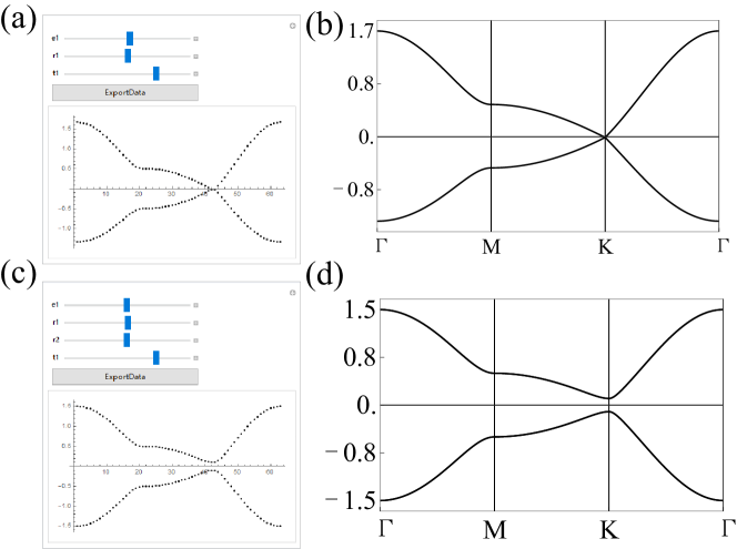
Figure 2: Output of bandManipulate and bandplot for graphene without considering spin (a-b) and with spin (c-d).

Moreover we can get the wannier90_hr.dat by hop function for this model.

⬇

hop[hamsoc, {e1 -> 0, r1 -> 0.02, r2 -> 0, t1 -> 0.5}]

Generated by MagneticTB

4

7

1 1 1 1 1 1 1

-1 -1 0 1 1 0.00000000 0.02000000

-1 -1 0 2 1 0.00000000 0.00000000

-1 -1 0 3 1 0.00000000 0.00000000

-1 -1 0 4 1 0.00000000 0.00000000

-1 -1 0 1 2 0.00000000 0.00000000

-1 -1 0 2 2 0.00000000 -0.02000000

…

4.3 Magnetic C-3 Weyl point

The charge-3 (C-3) Weyl point is a 0D two-fold band degeneracy with Chern number $|C|=3$. Encyclopedia of emergent particles tell us that the C-3 Weyl point always appear at least in a pair or coexist with nodal surface in nonmagnetic systems [51]. Here we confirm that in magnetic system, due to the breaking of time reversal symmetry ${\cal T}$, the C-3 Weyl point can uniquely coexist with conventional Weyl points. Consider the type IV magnetic space group $P_{c}3$ (BNS No. 143.3). The generator of the group is $C_{3z}$ and $\{E|00\frac{1}{2}\}{\cal T}$, Put $\ket{p_{x}+ip_{y}\uparrow},\ket{p_{x}-ip_{y}\downarrow}$ basis functions at Wyckoff position $2a$, and then the symmetry operator for $C_{3z}$ and $E\{00\frac{1}{2}\}{\cal T}$ are

$$\begin{split}C_{3z}&=-\sigma_{z}\\ \{E|00\frac{1}{2}\}{\cal T}&=i\sigma_{y}\end{split}$$

Under this bases the effective Hamiltonian at $\Gamma$ point can be written as

$$H_{\text{C-3\ WP}} = \epsilon+\alpha k_{z}\sigma_{x}+ck_{\parallel}^{2}+\beta(k_{x}+e^{-i\frac{\pi}{3}}k_{y})^{3}\sigma_{z}+h.c.$$ (18)

where $\epsilon,c$ are real parameters and $\alpha,\beta$ are complex parameters. Besides, there are another three essential Weyl points locate at $(\pi,0,0),(0,\pi,0),(\pi,\pi,0)$. Since the $C_{3z}$ symmetry does not change the Chern number of Weyl points, the Chern number at $M$ has to be $\pm 1$. According to no-go theorem, the Chern number of $\Gamma$ is $\mp 3$. One can easily check that the Chern number of Eq. (18) is $\pm 3$. The degeneracies of $\Gamma$ and $M$ are because $(\{E|00\frac{1}{2}\}{\cal T})^{2}=-1$ at $(0/\pi,0/\pi,0)$. The model can be obtained as follow

⬇

sgop = msgop[bnsdict[{143, 3}]];

init[lattice -> {{Sqrt[3]/2, -( 1/2), 0}, {0, 1, 0}, {0, 0, 2}},

lattpar -> {},

wyckoffposition -> {{{0, 0, 0}, {0, 0, 1}}},

symminformation -> sgop,

basisFunctions -> {{{x + I y, 0}, {0, x - I y}}}];

c3w = Sum[symham[i], {i, {2, 4}}];

c3w2band = Table[c3w[[i, j]], {i, {1, 4}}, {j, {1, 4}}];

The band structure of c3w2band is shown in Fig. 3(a).

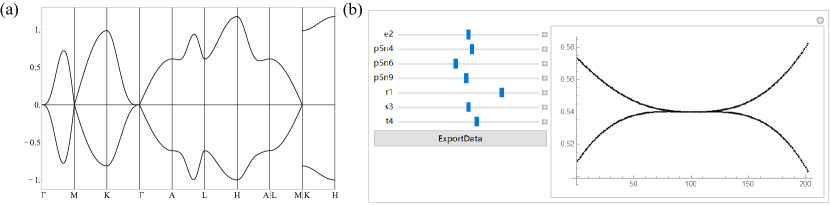
Figure 3: (a) Output of bandplot for magnetic C-3 Weyl point, (b) Output of bandManipulate for magnetic cubic nodal-line.

4.4 Magnetic cubic nodal-line

Topological high order nodal line is that the energy difference between the bands are non-linear,and the order of energy dispersion around the degeneracy points plays an important role in different physical properties, such as density of states, Berry phase and Landau-level [52]. Recently, Zhang et. al. proposed high order nodal-line in magnetic system [53]. In this example, we use MagneticTB to generate magnetic cubic nodal-line. Generally, the magnetic cubic nodal-line is protected by $C_{6z}$ and $M_{x}$ symmetries, there are many magnetic space groups which contains the above two symmetries. Consider the type IV magnetic space group $P_{c}6cc$ (BNS No. 184.196), and put $\ket{p_{x}+ip_{y}\uparrow},\ket{p_{x}-ip_{y}\downarrow}$ basis functions at Wyckoff position $2a$. Then the tight-binding model can be generated by

⬇

sgop = msgop[bnsdict[{184, 196}]];

init[lattice -> {{Sqrt[3]/2, -1/2, 0}, {0, 1, 0}, {0, 0, 2}},

lattpar -> {},

wyckoffposition -> {{{0, 0, 0}, {0, 0, 1}}},

symminformation -> sgop,

basisFunctions -> {{{x + I y, 0}, {0, x - I y}}}];

cnl = Sum[symham[i, symmetryset -> {2, 7, 13}], {i, 1, 5}];

cnl2band = Table[cnl[[i, j]], {i, {1, 4}}, {j, {1, 4}}];

MatrixForm[cnl2band]

path = {{

{{0, 1/10, 1/4}, {0, 0, 1/4}}, {"Q", "P"}},

{{{0, 0, 1/4}, {-1/10, 1/10, 1/4}}, {"P", "Q"}}};

bandManipulate[path, 20, cnl2band]

One can check that no mater how the parameters change, the dispersion of arbitrary point along $\Gamma$-$A$ on $k_{x}$-$k_{y}$ plane are non-linear, see Fig. 3(b) which is consistent with Ref. [53].

5 Conclusion

In conclusion, we have developed a software package to generate the symmetry-adopted tight-binding model for arbitrary magnetic space group. The input parameters for MagneticTB are clear and easy to set and both spinless and spinful Hamiltonian can be generated automatically. Besides, some useful functions such as manipulating the band structure, interfacing with other software are implemented, which can be used for further study on the magnetic systems. Moreover, MagneticTB can not only be used to investigate physical properties of electronic systems, but also be used to study photonics, ultracold, acoustic and mechanical systems [54, 55, 56]. Finally, an exciting direction for future is to apply the magnetic field for the tight-binding model in MagneticTB [57].

Appendix A

In this appendix, we use the translation operation $T(\bm{d})$. For $Q=\{R|\bm{v}\}$, we have $QT(\bm{d})=\{R|\bm{v}\}\{E|\bm{d}\}=\{R|R\bm{d}+\bm{v}\}=T(Q\bm{d})R$. Thus

$$\begin{split}E(\bm{d}_{j}^{n},(\bm{R}_{j}+\bm{d}_{l^{\prime}}^{n^{\prime}}))&=\braket{\hat{T}(\bm{d}_{l}^{n})\varPhi^{n}(\bm{r})}{\hat{Q}^{\dagger}\hat{H}\hat{Q}}{\hat{T}(\bm{d}_{l^{\prime}}^{n^{\prime}}+\bm{R}_{j})\varPhi^{n^{\prime}}(\bm{r})}\\ &=\braket{\hat{Q}\hat{T}(\bm{d}_{l}^{n})\varPhi^{n}(\bm{r})}{\hat{H}}{\hat{Q}\hat{T}(\bm{d}_{l^{\prime}}^{n^{\prime}}+\bm{R}_{j})\varPhi^{n^{\prime}}(\bm{r})}\\ &=\braket{\hat{T}(Q\bm{d}_{l}^{n})R\varPhi^{n}(\bm{r})}{\hat{H}}{\hat{T}(Q(\bm{d}_{l^{\prime}}^{n^{\prime}}+\bm{R}_{j}))R\varPhi^{n^{\prime}}(\bm{r})}\\ &=D^{n\dagger}(R)\braket{\hat{T}(Q\bm{d}_{l}^{n})\varPhi^{n}(\bm{r})}{\hat{H}}{\hat{T}(Q(\bm{d}_{l^{\prime}}^{n^{\prime}}+\bm{R}_{j}))\varPhi^{n^{\prime}}(\bm{r})}D^{n^{\prime}}(R)\\ &=D^{n\dagger}(R)E(Q\bm{d}_{j}^{n},Q(\bm{R}_{j}+\bm{d}_{l^{\prime}}^{n^{\prime}}))D^{n^{\prime}}(R)\end{split}$$ (19)

which completes the proof of Eq.(5).

For $Q=\{R|\bm{v}\}{\cal T}$, notice time reversal symmetry does not change the real space coordinates, i.e. ${\cal T}\bm{d}=\bm{d}$, we have $QT(\bm{d})=\{R|\bm{v}\}{\cal T}\{E|\bm{d}\}=\{R|R\bm{d}+\bm{v}\}{\cal T}=T(Q\bm{d})R{\cal T}$. Use the fact that for anti-unitary operator $\hat{{\cal A}}$, $\braket{\hat{{\cal A}}\psi}{\hat{{\cal A}}\phi}=\braket{\psi}{\phi}^{*}$, then

$$\begin{split}E^{*}(\bm{d}_{j}^{n},(\bm{R}_{j}+\bm{d}_{l^{\prime}}^{n^{\prime}}))&=\braket{\hat{Q}\hat{T}(\bm{d}_{l}^{n})\varPhi^{n}(\bm{r})}{\hat{Q}\hat{H}}{\hat{T}(\bm{d}_{l^{\prime}}^{n^{\prime}}+\bm{R}_{j})\varPhi^{n^{\prime}}(\bm{r})}\\ &=\braket{\hat{Q}\hat{T}(\bm{d}_{l}^{n})\varPhi^{n}(\bm{r})}{\hat{H}}{\hat{Q}\hat{T}(\bm{d}_{l^{\prime}}^{n^{\prime}}+\bm{R}_{j})\varPhi^{n^{\prime}}(\bm{r})}\\ &=\braket{\hat{T}(Q\bm{d}_{l}^{n})R{\cal T}\varPhi^{n}(\bm{r})}{\hat{H}}{\hat{T}(Q(\bm{d}_{l^{\prime}}^{n^{\prime}}+\bm{R}_{j}))R{\cal T}\varPhi^{n^{\prime}}(\bm{r})}\\ &=D^{n\dagger}(R{\cal T})\braket{\hat{T}(Q\bm{d}_{l}^{n})\varPhi^{n}(\bm{r})}{\hat{H}}{\hat{T}(Q(\bm{d}_{l^{\prime}}^{n^{\prime}}+\bm{R}_{j}))\varPhi^{n^{\prime}}(\bm{r})}D^{n^{\prime}}(R{\cal T})\\ &=D^{n\dagger}(R{\cal T})E(Q\bm{d}_{j}^{n},Q(\bm{R}_{j}+\bm{d}_{l^{\prime}}^{n^{\prime}}))D^{n^{\prime}}(R{\cal T})\end{split}$$ (20)

which completes the proof of Eq.(6).

Proof of Eq.(13),

$$\begin{split}[H(\bm{k})P(Q)]_{ll^{\prime}}^{nn^{\prime}}&=\sum_{\mu\nu}H(\bm{k})_{l\mu}^{n\nu}P_{\mu l^{\prime}}^{\nu n^{\prime}}(Q)\\ &=\sum_{\mu\nu}\sum_{\bm{R}_{j}}e^{i\bm{k}\cdot(\bm{R}_{j}+\bm{d}_{\mu}^{\nu}-\bm{d}_{l}^{n})}E(\bm{d}_{l}^{n},\bm{R}_{j}+\bm{d}_{\mu}^{\nu})\delta_{\nu n^{\prime}}\delta_{\bm{d}_{\mu}^{\nu},Q\bm{d}_{l^{\prime}}^{n^{\prime}}+\bm{R}_{s}}D^{n^{\prime}}(R)\\ &=\sum_{\bm{R}_{j}}e^{i\bm{k}\cdot(\bm{R}_{j}+Q\bm{d}_{l^{\prime}}^{n^{\prime}}+\bm{R}_{s}-\bm{d}_{l}^{n})}E(\bm{d}_{l}^{n},\bm{R}_{j}+Q\bm{d}_{l^{\prime}}^{n^{\prime}}+\bm{R}_{s})D^{n^{\prime}}(R)\\ &\xlongequal{\bm{R}_{j}+\bm{R}_{s}\rightarrow R\bm{R}_{j}}\sum_{\bm{R}_{j}}e^{i\bm{k}\cdot R(\bm{R}_{j}+\bm{d}_{l^{\prime}}^{n^{\prime}}-Q^{-1}\bm{d}_{l}^{n})}E(\bm{d}_{l}^{n},Q(\bm{R}_{j}+\bm{d}_{l^{\prime}}^{n^{\prime}}))D^{n^{\prime}}(R)\\ &\xlongequal{\text{use Eq. (\ref{eq:hopp})}}\sum_{\bm{R}_{j}}e^{iR^{-1}\bm{k}\cdot(\bm{R}_{j}+\bm{d}_{l^{\prime}}^{n^{\prime}}-Q^{-1}\bm{d}_{l}^{n})}D^{n}(R)E(Q^{-1}\bm{d}_{l}^{n},\bm{R}_{j}+\bm{d}_{l^{\prime}}^{n^{\prime}})\end{split}$$ (21)

$$\begin{split}[P(Q)H(R^{-1}\bm{k})]_{ll^{\prime}}^{nn^{\prime}}&=\sum_{\mu\nu}P_{l\mu}^{n\nu}(Q)H(R^{-1}\bm{k})_{\mu l^{\prime}}^{\nu n^{\prime}}\\ &=\sum_{\mu\nu}\sum_{\bm{R}_{j}}\delta_{n\nu}\delta_{\bm{d}_{l}^{n},Q\bm{d}_{\mu}^{\nu}+\bm{R}_{s}}D^{n}(R)e^{iR^{-1}\bm{k}\cdot(\bm{R}_{j}+\bm{d}_{l^{\prime}}^{n^{\prime}}-\bm{d}_{\mu}^{\nu})}E(\bm{d}_{\mu}^{\nu},\bm{R}_{j}+\bm{d}_{l^{\prime}}^{n^{\prime}})\\ &=\sum_{\bm{R}_{j}}D^{n}(R)e^{iR^{-1}\bm{k}\cdot(\bm{R}_{j}+\bm{d}_{l^{\prime}}^{n^{\prime}}-Q^{-1}(\bm{d}_{l}^{n}-\bm{R}_{s}))}E(Q^{-1}(\bm{d}_{l}^{n}-\bm{R}_{s}),\bm{R}_{j}+\bm{d}_{l^{\prime}}^{n^{\prime}})\\ &=\sum_{\bm{R}_{j}}e^{iR^{-1}\bm{k}\cdot(\bm{R}_{j}+\bm{d}_{l^{\prime}}^{n^{\prime}}-Q^{-1}\bm{d}_{l}^{n}+R^{-1}\bm{R}_{s})}D^{n}(R)E(Q^{-1}\bm{d}_{l}^{n}-R^{-1}\bm{R}_{s},\bm{R}_{j}+\bm{d}_{l^{\prime}}^{n^{\prime}})\\ &=\sum_{\bm{R}_{j}}e^{iR^{-1}\bm{k}\cdot(\bm{R}_{j}+\bm{d}_{l^{\prime}}^{n^{\prime}}-Q^{-1}\bm{d}_{l}^{n}+R^{-1}\bm{R}_{s})}D^{n}(R)E(Q^{-1}\bm{d}_{l}^{n},\bm{R}_{j}+\bm{d}_{l^{\prime}}^{n^{\prime}}+R^{-1}\bm{R}_{s})\\ &\xlongequal{\bm{R}_{j}+R^{-1}\bm{R}_{s}\rightarrow\bm{R}_{j}}\sum_{\bm{R}_{j}}e^{iR^{-1}\bm{k}\cdot(\bm{R}_{j}+\bm{d}_{l^{\prime}}^{n^{\prime}}-Q^{-1}\bm{d}_{l}^{n})}D^{n}(R)E(Q^{-1}\bm{d}_{l}^{n},\bm{R}_{j}+\bm{d}_{l^{\prime}}^{n^{\prime}})\end{split}$$ (22)

In the above derivation we use the relation $Q^{-1}(\bm{d}_{l}^{n}-\bm{R}_{s})=Q^{-1}\bm{d}_{l}^{n}-R^{-1}\bm{R}_{s}$ ($Q^{-1}$ is not linear). Compare the last lines of the above two equations and we can find they are equal to each other, i.e.

$$[H(\bm{k})P(Q)]_{ll^{\prime}}^{nn^{\prime}}=[P(Q)H(R^{-1}\bm{k})]_{ll^{\prime}}^{nn^{\prime}}\ \ \ \ \ \Rightarrow\ \ \ \ \ H(\bm{k})P(Q)=P(Q)H(R^{-1}\bm{k})$$ (23)

Proof of Eq.(14): similar to Eq.(21) and Eq.(22) we have

$$\begin{split}[H(\bm{k})P(Q)]_{ll^{\prime}}^{nn^{\prime}}&=\sum_{\mu\nu}H(\bm{k})_{l\mu}^{n\nu}P_{\mu l^{\prime}}^{\nu n^{\prime}}(Q)\\ &=\sum_{\mu\nu}\sum_{\bm{R}_{j}}e^{i\bm{k}\cdot(\bm{R}_{j}+\bm{d}_{\mu}^{\nu}-\bm{d}_{l}^{n})}E(\bm{d}_{l}^{n},\bm{R}_{j}+\bm{d}_{\mu}^{\nu})\delta_{\nu n^{\prime}}\delta_{\bm{d}_{\mu}^{\nu},Q\bm{d}_{l^{\prime}}^{n^{\prime}}+\bm{R}_{s}}D^{n^{\prime}}(R\mathcal{T})\\ &=\sum_{\bm{R}_{j}}e^{i\bm{k}\cdot(\bm{R}_{j}+Q\bm{d}_{l^{\prime}}^{n^{\prime}}+\bm{R}_{s}-\bm{d}_{l}^{n})}E(\bm{d}_{l}^{n},\bm{R}_{j}+Q\bm{d}_{l^{\prime}}^{n^{\prime}}+\bm{R}_{s})D^{n^{\prime}}(R\mathcal{T})\\ &\xlongequal{\bm{R}_{j}+\bm{R}_{s}\rightarrow R\bm{R}_{j}}\sum_{\bm{R}_{j}}e^{i\bm{k}\cdot R(\bm{R}_{j}+\bm{d}_{l^{\prime}}^{n^{\prime}}-Q^{-1}\bm{d}_{l}^{n})}E(\bm{d}_{l}^{n},Q(\bm{R}_{j}+\bm{d}_{l^{\prime}}^{n^{\prime}}))D^{n^{\prime}}(R\mathcal{T})\\ &\xlongequal{\text{use Eq. (\ref{eq:hopptri})}}\sum_{\bm{R}_{j}}e^{iR^{-1}\bm{k}\cdot(\bm{R}_{j}+\bm{d}_{l^{\prime}}^{n^{\prime}}-Q^{-1}\bm{d}_{l}^{n})}D^{n}(R\mathcal{T})E^{*}(Q^{-1}\bm{d}_{l}^{n},\bm{R}_{j}+\bm{d}_{l^{\prime}}^{n^{\prime}})\end{split}$$ (24)

$$\begin{split}[P(Q)H^{*}(-R^{-1}\bm{k})]_{ll^{\prime}}^{nn^{\prime}}&=\sum_{\mu\nu}P_{l\mu}^{n\nu}(Q)H^{*}(-R^{-1}\bm{k})_{\mu l^{\prime}}^{\nu n^{\prime}}\\ &=\sum_{\mu\nu}\sum_{\bm{R}_{j}}\delta_{n\nu}\delta_{\bm{d}_{l}^{n},Q\bm{d}_{\mu}^{\nu}+\bm{R}_{s}}D^{n}(R\mathcal{T})e^{iR^{-1}\bm{k}\cdot(\bm{R}_{j}+\bm{d}_{l^{\prime}}^{n^{\prime}}-\bm{d}_{\mu}^{\nu})}E^{*}(\bm{d}_{\mu}^{\nu},\bm{R}_{j}+\bm{d}_{l^{\prime}}^{n^{\prime}})\\ &=\sum_{\bm{R}_{j}}D^{n}(R\mathcal{T})e^{iR^{-1}\bm{k}\cdot(\bm{R}_{j}+\bm{d}_{l^{\prime}}^{n^{\prime}}-Q^{-1}(\bm{d}_{l}^{n}-\bm{R}_{s}))}E^{*}(Q^{-1}(\bm{d}_{l}^{n}-\bm{R}_{s}),\bm{R}_{j}+\bm{d}_{l^{\prime}}^{n^{\prime}})\\ &=\sum_{\bm{R}_{j}}e^{iR^{-1}\bm{k}\cdot(\bm{R}_{j}+\bm{d}_{l^{\prime}}^{n^{\prime}}-Q^{-1}\bm{d}_{l}^{n}+R^{-1}\bm{R}_{s})}D^{n}(R\mathcal{T})E^{*}(Q^{-1}\bm{d}_{l}^{n}-R^{-1}\bm{R}_{s},\bm{R}_{j}+\bm{d}_{l^{\prime}}^{n^{\prime}})\\ &=\sum_{\bm{R}_{j}}e^{iR^{-1}\bm{k}\cdot(\bm{R}_{j}+\bm{d}_{l^{\prime}}^{n^{\prime}}-Q^{-1}\bm{d}_{l}^{n}+R^{-1}\bm{R}_{s})}D^{n}(R\mathcal{T})E^{*}(Q^{-1}\bm{d}_{l}^{n},\bm{R}_{j}+\bm{d}_{l^{\prime}}^{n^{\prime}}+R^{-1}\bm{R}_{s})\\ &\xlongequal{\bm{R}_{j}+R^{-1}\bm{R}_{s}\rightarrow\bm{R}_{j}}\sum_{\bm{R}_{j}}e^{iR^{-1}\bm{k}\cdot(\bm{R}_{j}+\bm{d}_{l^{\prime}}^{n^{\prime}}-Q^{-1}\bm{d}_{l}^{n})}D^{n}(R\mathcal{T})E^{*}(Q^{-1}\bm{d}_{l}^{n},\bm{R}_{j}+\bm{d}_{l^{\prime}}^{n^{\prime}})\end{split}$$ (25)

Compare the last lines of the above two equations and we can find they are equal to each other, i.e.

$$[H(\bm{k})P(Q)]_{ll^{\prime}}^{nn^{\prime}}=[P(Q)H^{*}(-R^{-1}\bm{k})]_{ll^{\prime}}^{nn^{\prime}}\ \ \ \ \ \Rightarrow\ \ \ \ \ H(\bm{k})P(Q)=P(Q)H^{*}(-R^{-1}\bm{k})$$ (26)

It is easy to verify that for $A,B$ not containing ${\cal T}$ and $C,D$ containing ${\cal T}$, $P(Q)$ obey the following corepresentation algebra:

$$\begin{split}P(A)P(B)&=P(AB)\\ P(A)P(C)&=P(AC)\\ P(C)P^{*}(A)&=P(CA)\\ P(C)P^{*}(D)&=P(CD)\end{split}$$ (27)

References

- Wallace [1947] P. R. Wallace, The Band Theory of Graphite, Phys. Rev. 71 (1947) 622–634. URL: https://link.aps.org/doi/10.1103/PhysRev.71.622. doi:10.1103/PhysRev.71.622, publisher: American Physical Society.
- Löwdin [1950] P.-O. Löwdin, On the Non-Orthogonality Problem Connected with the Use of Atomic Wave Functions in the Theory of Molecules and Crystals, J. Chem. Phys. 18 (1950) 365–375. URL: https://aip.scitation.org/doi/10.1063/1.1747632. doi:10.1063/1.1747632, publisher: American Institute of Physics.
- Slater and Koster [1954] J. C. Slater, G. F. Koster, Simplified LCAO Method for the Periodic Potential Problem, Phys. Rev. 94 (1954) 1498–1524. URL: https://link.aps.org/doi/10.1103/PhysRev.94.1498. doi:10.1103/PhysRev.94.1498, publisher: American Physical Society.
- Goringe et al. [1997] C. M. Goringe, D. R. Bowler, E. Hernández, Tight-binding modelling of materials, Rep. Prog. Phys. 60 (1997) 1447. URL: https://iopscience.iop.org/article/10.1088/0034-4885/60/12/001/meta. doi:10.1088/0034-4885/60/12/001, publisher: IOP Publishing.
- Wieder et al. [2018] B. J. Wieder, B. Bradlyn, Z. Wang, J. Cano, Y. Kim, H.-S. D. Kim, A. M. Rappe, C. L. Kane, B. A. Bernevig, Wallpaper fermions and the nonsymmorphic Dirac insulator, Science 361 (2018) 246–251. URL: http://www.sciencemag.org/lookup/doi/10.1126/science.aan2802. doi:10.1126/science.aan2802.
- Kane and Mele [2005] C. L. Kane, E. J. Mele, Z Topological Order and the Quantum Spin Hall Effect, Phys. Rev. Lett. 95 (2005) 146802. URL: http://link.aps.org/doi/10.1103/PhysRevLett.95.146802. doi:10.1103/PhysRevLett.95.146802.
- Fu [2011] L. Fu, Topological Crystalline Insulators, Phys. Rev. Lett. 106 (2011) 106802. URL: https://link.aps.org/doi/10.1103/PhysRevLett.106.106802. doi:10.1103/PhysRevLett.106.106802.
- Burkov et al. [2011] A. A. Burkov, M. D. Hook, L. Balents, Topological nodal semimetals, Phys. Rev. B 84 (2011) 235126. URL: https://link.aps.org/doi/10.1103/PhysRevB.84.235126. doi:10.1103/PhysRevB.84.235126.
- Fang et al. [2013] C. Fang, M. J. Gilbert, B. A. Bernevig, Topological insulators with commensurate antiferromagnetism, Phys. Rev. B 88 (2013) 085406. URL: https://link.aps.org/doi/10.1103/PhysRevB.88.085406. doi:10.1103/PhysRevB.88.085406.
- Liu [2013] C.-X. Liu, Antiferromagnetic crystalline topological insulators, arXiv:1304.6455 [cond-mat] (2013). URL: http://arxiv.org/abs/1304.6455, arXiv: 1304.6455.
- Egorov et al. [1968] R. F. Egorov, B. I. Reser, V. P. Shirokovskii, Consistent Treatment of Symmetry in the Tight Binding Approximation, Physica Status Solidi B 26 (1968) 391–408. URL: http://doi.wiley.com/10.1002/pssb.19680260202. doi:10.1002/pssb.19680260202.
- Kuznetsov and Men [1978] V. N. Kuznetsov, A. N. Men, Symmetry and analytical expressions of matrix components in the tight-binding method, Physica Status Solidi B 85 (1978) 95–104. URL: http://doi.wiley.com/10.1002/pssb.2220850109. doi:10.1002/pssb.2220850109.
- Ku et al. [2002] W. Ku, H. Rosner, W. E. Pickett, R. T. Scalettar, Insulating Ferromagnetism in La4Ba2Cu2O10 : An Ab Initio Wannier Function Analysis, Phys. Rev. Lett. 89 (2002) 167204. URL: https://link.aps.org/doi/10.1103/PhysRevLett.89.167204. doi:10.1103/PhysRevLett.89.167204.
- Liu et al. [2013] G.-B. Liu, W.-Y. Shan, Y. Yao, W. Yao, D. Xiao, Three-band tight-binding model for monolayers of group-VIB transition metal dichalcogenides, Phys. Rev. B 88 (2013) 085433. URL: https://link.aps.org/doi/10.1103/PhysRevB.88.085433. doi:10.1103/PhysRevB.88.085433.
- Wieder and Kane [2016] B. J. Wieder, C. L. Kane, Spin-orbit semimetals in the layer groups, Phys. Rev. B 94 (2016) 155108. URL: https://link.aps.org/doi/10.1103/PhysRevB.94.155108. doi:10.1103/PhysRevB.94.155108.
- Wang et al. [2016] Z. Wang, A. Alexandradinata, R. J. Cava, B. A. Bernevig, Hourglass fermions, Nature 532 (2016) 189. URL: https://www.nature.com/articles/nature17410. doi:10.1038/nature17410.
- Song et al. [2017] Z. Song, Z. Fang, C. Fang, (-2) -Dimensional Edge States of Rotation Symmetry Protected Topological States, Phys. Rev. Lett. 119 (2017) 246402. URL: https://link.aps.org/doi/10.1103/PhysRevLett.119.246402. doi:10.1103/PhysRevLett.119.246402.
- Zhang et al. [2018] Z. Zhang, Q. Gao, C.-C. Liu, H. Zhang, Y. Yao, Magnetization-direction tunable nodal-line and Weyl phases, Phys. Rev. B 98 (2018) 121103(R). URL: https://link.aps.org/doi/10.1103/PhysRevB.98.121103. doi:10.1103/PhysRevB.98.121103.
- Gresch et al. [2018] D. Gresch, Q. Wu, G. W. Winkler, R. Häuselmann, M. Troyer, A. A. Soluyanov, Automated construction of symmetrized Wannier-like tight-binding models from ab initio calculations, Phys. Rev. Materials 2 (2018) 103805. URL: https://link.aps.org/doi/10.1103/PhysRevMaterials.2.103805. doi:10.1103/PhysRevMaterials.2.103805.
- Koshino et al. [2018] M. Koshino, N. F. Q. Yuan, T. Koretsune, M. Ochi, K. Kuroki, L. Fu, Maximally Localized Wannier Orbitals and the Extended Hubbard Model for Twisted Bilayer Graphene, Phys. Rev. X 8 (2018). URL: https://link.aps.org/doi/10.1103/PhysRevX.8.031087. doi:10.1103/PhysRevX.8.031087.
- Yu et al. [2019] Z.-M. Yu, W. Wu, Y. X. Zhao, S. A. Yang, Circumventing the no-go theorem: A single Weyl point without surface Fermi arcs, Phys. Rev. B 100 (2019) 041118. URL: https://link.aps.org/doi/10.1103/PhysRevB.100.041118. doi:10.1103/PhysRevB.100.041118, publisher: American Physical Society.
- Di Martino et al. [1999] B. Di Martino, M. Celino, V. Rosato, An high performance Fortran implementation of a Tight-Binding Molecular Dynamics simulation, Comput. Phys. Commun. 120 (1999) 255–268. URL: https://linkinghub.elsevier.com/retrieve/pii/S0010465599002519. doi:10.1016/S0010-4655(99)00251-9.
- Groth [2014] C. W. Groth, Kwant: a software package for quantum transport, New J. Phys. (2014) 40.
- Supka et al. [2017] A. R. Supka, T. E. Lyons, L. Liyanage, P. D’Amico, R. Al Rahal Al Orabi, S. Mahatara, P. Gopal, C. Toher, D. Ceresoli, A. Calzolari, S. Curtarolo, M. B. Nardelli, M. Fornari, AFLOW: A minimalist approach to high-throughput ab initio calculations including the generation of tight-binding hamiltonians, Comput. Mater. Sci. 136 (2017) 76–84. URL: http://www.sciencedirect.com/science/article/pii/S0927025617301970. doi:10.1016/j.commatsci.2017.03.055.
- Nakhaee et al. [2020] M. Nakhaee, S. A. Ketabi, F. M. Peeters, Tight-Binding Studio: A technical software package to find the parameters of tight-binding Hamiltonian, Comput. Phys. Commun. 254 (2020) 107379. URL: https://linkinghub.elsevier.com/retrieve/pii/S0010465520301636. doi:10.1016/j.cpc.2020.107379.
- Klymenko et al. [2021] M. Klymenko, J. Vaitkus, J. Smith, J. Cole, NanoNET: An extendable Python framework for semi-empirical tight-binding models, Comput. Phys. Commun. 259 (2021) 107676. URL: https://linkinghub.elsevier.com/retrieve/pii/S0010465520303283. doi:10.1016/j.cpc.2020.107676.
- Mostofi et al. [2008] A. A. Mostofi, J. R. Yates, Y.-S. Lee, I. Souza, D. Vanderbilt, N. Marzari, Wannier90: A Tool for Obtaining Maximally-Localised Wannier Functions, Comput. Phys. Commun. 178 (2008) 685. URL: http://arxiv.org/abs/0708.0650. doi:10.1016/j.cpc.2007.11.016, arXiv: 0708.0650.
- Giannozzi et al. [2009] P. Giannozzi, S. Baroni, N. Bonini, M. Calandra, R. Car, C. Cavazzoni, D. Ceresoli, G. L. Chiarotti, M. Cococcioni, I. Dabo, A. D. Corso, S. d. Gironcoli, S. Fabris, G. Fratesi, R. Gebauer, U. Gerstmann, C. Gougoussis, A. Kokalj, M. Lazzeri, L. Martin-Samos, N. Marzari, F. Mauri, R. Mazzarello, S. Paolini, A. Pasquarello, L. Paulatto, C. Sbraccia, S. Scandolo, G. Sclauzero, A. P. Seitsonen, A. Smogunov, P. Umari, R. M. Wentzcovitch, QUANTUM ESPRESSO: a modular and open-source software project for quantum simulations of materials, J. Phys. Condens. Matter 21 (2009) 395502. URL: https://doi.org/10.1088/0953-8984/21/39/395502. doi:10.1088/0953-8984/21/39/395502, publisher: IOP Publishing.
- Kresse and Furthmüller [1996] G. Kresse, J. Furthmüller, Efficient iterative schemes for ab initio total-energy calculations using a plane-wave basis set, Phys. Rev. B 54 (1996) 11169–11186. URL: https://link.aps.org/doi/10.1103/PhysRevB.54.11169. doi:10.1103/PhysRevB.54.11169, publisher: American Physical Society.
- Gonze et al. [2009] X. Gonze, B. Amadon, P. M. Anglade, J. M. Beuken, F. Bottin, P. Boulanger, F. Bruneval, D. Caliste, R. Caracas, M. Côté, T. Deutsch, L. Genovese, P. Ghosez, M. Giantomassi, S. Goedecker, D. R. Hamann, P. Hermet, F. Jollet, G. Jomard, S. Leroux, M. Mancini, S. Mazevet, M. J. T. Oliveira, G. Onida, Y. Pouillon, T. Rangel, G. M. Rignanese, D. Sangalli, R. Shaltaf, M. Torrent, M. J. Verstraete, G. Zerah, J. W. Zwanziger, ABINIT: First-principles approach to material and nanosystem properties, Comput. Phys. Commun. 180 (2009) 2582–2615. URL: http://www.sciencedirect.com/science/article/pii/S0010465509002276. doi:10.1016/j.cpc.2009.07.007.
- Koepernik and Eschrig [1999] K. Koepernik, H. Eschrig, Full-potential nonorthogonal local-orbital minimum-basis band-structure scheme, Phys. Rev. B 59 (1999) 1743–1757. URL: https://link.aps.org/doi/10.1103/PhysRevB.59.1743. doi:10.1103/PhysRevB.59.1743, publisher: American Physical Society.
- Hergert and Geilhufe [2018] W. Hergert, R. Geilhufe, Group Theory in Solid State Physics and Photonics: Problem Solving with Mathematica, Wiley-VCH Verlag GmbH & Co. KGaA, Weinheim, Germany, 2018. URL: http://doi.wiley.com/10.1002/9783527695799. doi:10.1002/9783527695799.
- Varjas et al. [2018] D. Varjas, T. Ö. Rosdahl, A. R. Akhmerov, Qsymm: algorithmic symmetry finding and symmetric Hamiltonian generation, New Journal of Physics 20 (2018) 093026. URL: https://doi.org/10.1088/1367-2630/aadf67. doi:10.1088/1367-2630/aadf67, publisher: IOP Publishing.
- Jacobse [2019] P. H. Jacobse, MathemaTB: A Mathematica package for tight-binding calculations, Comput. Phys. Commun. 244 (2019) 392–408. URL: https://linkinghub.elsevier.com/retrieve/pii/S0010465519301821. doi:10.1016/j.cpc.2019.06.003.
- Wu et al. [2018] Q. Wu, S. Zhang, H.-F. Song, M. Troyer, A. A. Soluyanov, WannierTools: An open-source software package for novel topological materials, Comput. Phys. Commun. 224 (2018) 405–416. URL: http://arxiv.org/abs/1703.07789. doi:10.1016/j.cpc.2017.09.033.
- Cloizeaux [1963] J. D. Cloizeaux, Orthogonal Orbitals and Generalized Wannier Functions, Phys. Rev. 129 (1963) 554–566. URL: https://link.aps.org/doi/10.1103/PhysRev.129.554. doi:10.1103/PhysRev.129.554, publisher: American Physical Society.
- LANDAU and LIFSHITZ [1977] L. D. LANDAU, E. M. LIFSHITZ, CHAPTER VIII - SPIN, in: L. D. LANDAU, E. M. LIFSHITZ (Eds.), Quantum Mechanics (Third Edition), third edition ed., Pergamon, 1977, pp. 197–224. URL: https://www.sciencedirect.com/science/article/pii/B9780080209401500153. doi:10.1016/B978-0-08-020940-1.50015-3.
- Liu et al. [2021] G.-B. Liu, M. Chu, Z. Zhang, Z.-M. Yu, Y. Yao, SpaceGroupIrep: A package for irreducible representations of space group, Comput. Phys. Commun. 265 (2021) 107993. URL: https://linkinghub.elsevier.com/retrieve/pii/S0010465521001053. doi:10.1016/j.cpc.2021.107993.
- Zhang and et. al. [2021] Z. Zhang, et. al., Database for tight-binding model with magnetic symmetry (in preparation) (2021).
- Litvin [2014] D. B. Litvin, 1-, 2- and 3-Dimensional Magnetic Subperiodic Groups and Magnetic Space Groups, 2014. URL: https://www.iucr.org/publ/978-0-9553602-2-0.
- Stokes et al. [2021] H. T. Stokes, D. M. Hatch, B. J. Campbell, ISOTROPY Software Suite (2021). URL: iso.byu.edu.
- Bradley and Cracknell [1972] C. Bradley, A. Cracknell, The Mathematical Theory of Symmetry in Solids: Representation Theory for Point Groups and Space Groups, Oxford University Press, New York, 1972.
- Dresselhaus et al. [2008] M. S. Dresselhaus, G. Dresselhaus, A. Jorio, Group theory: application to the physics of condensed matter, Springer-Verlag, Berlin, 2008.
- Gresch et al. [2017] D. Gresch, G. Autès, O. V. Yazyev, M. Troyer, D. Vanderbilt, B. A. Bernevig, A. A. Soluyanov, Z2Pack: Numerical implementation of hybrid Wannier centers for identifying topological materials, Phys. Rev. B 95 (2017) 075146. URL: https://link.aps.org/doi/10.1103/PhysRevB.95.075146. doi:10.1103/PhysRevB.95.075146.
- Yusufaly et al. [2017] T. Yusufaly, D. Vanderbilt, S. Coh, Tight-Binding Formalism in the Context of the PythTB Package (2017).
- Zhang et al. [2018] Z. Zhang, R.-W. Zhang, X. Li, K. Koepernik, Y. Yao, H. Zhang, High-Throughput Screening and Automated Processing toward Novel Topological Insulators, J. Phys. Chem. Lett. 9 (2018) 6224. URL: http://pubs.acs.org/doi/10.1021/acs.jpclett.8b02800. doi:10.1021/acs.jpclett.8b02800.
- Li et al. [2018] X. Li, Z. Zhang, Y. Yao, H. Zhang, High throughput screening for two-dimensional topological insulators, 2D Mater. 5 (2018) 045023. URL: http://stacks.iop.org/2053-1583/5/i=4/a=045023?key=crossref.561297051e0e67968b784af6138a9275. doi:10.1088/2053-1583/aadb1e.
- Wang et al. [2012] Q. H. Wang, K. Kalantar-Zadeh, A. Kis, J. N. Coleman, M. S. Strano, Electronics and optoelectronics of two-dimensional transition metal dichalcogenides, Nat. Nanotechnol. 7 (2012) 699–712. URL: https://www.nature.com/articles/nnano.2012.193. doi:10.1038/nnano.2012.193, number: 11 Publisher: Nature Publishing Group.
- Liu et al. [2015] G.-B. Liu, D. Xiao, Y. Yao, X. Xu, W. Yao, Electronic structures and theoretical modelling of two-dimensional group-vib transition metal dichalcogenides, Chem. Soc. Rev. 44 (2015) 2643–2663. URL: http://dx.doi.org/10.1039/C4CS00301B. doi:10.1039/C4CS00301B.
- Castro Neto et al. [2009] A. H. Castro Neto, F. Guinea, N. M. R. Peres, K. S. Novoselov, A. K. Geim, The electronic properties of graphene, Rev. Mod. Phys. 81 (2009) 109–162. URL: https://link.aps.org/doi/10.1103/RevModPhys.81.109. doi:10.1103/RevModPhys.81.109.
- Yu et al. [2020] Z.-M. Yu, Z. Zhang, G.-B. Liu, W. Weikang, X.-P. Li, Z. Run-Wu, S. A. Yang, Y. Yao, Encyclopedia of emergent particles in three-dimensional crystals, arXiv:2102.01517 (2020).
- Yu et al. [2019] Z.-M. Yu, W. Wu, X.-L. Sheng, Y. X. Zhao, S. A. Yang, Quadratic and cubic nodal lines stabilized by crystalline symmetry, Phys. Rev. B 99 (2019) 121106(R). URL: https://link.aps.org/doi/10.1103/PhysRevB.99.121106. doi:10.1103/PhysRevB.99.121106.
- Zhang et al. [2021] Z. Zhang, Z.-M. Yu, S. A. Yang, Magnetic higher-order nodal lines, Phys. Rev. B 103 (2021) 115112. URL: https://link.aps.org/doi/10.1103/PhysRevB.103.115112. doi:10.1103/PhysRevB.103.115112.
- Ozawa et al. [2019] T. Ozawa, H. M. Price, A. Amo, N. Goldman, M. Hafezi, L. Lu, M. C. Rechtsman, D. Schuster, J. Simon, O. Zilberberg, I. Carusotto, Topological photonics, Rev. Mod. Phys. 91 (2019). URL: https://link.aps.org/doi/10.1103/RevModPhys.91.015006. doi:10.1103/RevModPhys.91.015006.
- Cooper et al. [2019] N. R. Cooper, J. Dalibard, I. B. Spielman, Topological bands for ultracold atoms, Rev. Mod. Phys. 91 (2019). URL: https://link.aps.org/doi/10.1103/RevModPhys.91.015005. doi:10.1103/RevModPhys.91.015005.
- Ma et al. [2019] G. Ma, M. Xiao, C. T. Chan, Topological phases in acoustic and mechanical systems, Nature Reviews Physics 1 (2019) 281–294. URL: https://www.nature.com/articles/s42254-019-0030-x. doi:10.1038/s42254-019-0030-x, number: 4 Publisher: Nature Publishing Group.
- Peierls [1933] R. Peierls, Zur Theorie des Diamagnetismus von Leitungselektronen, Zeitschrift für Physik 80 (1933) 763–791. URL: http://link.springer.com/10.1007/BF01342591. doi:10.1007/BF01342591.