Bayesian Calibration for Large-Scale Fluid Structure Interaction Problems Under Embedded/Immersed Boundary Framework

Abstract

[Abstract]

Bayesian calibration is widely used for inverse analysis and uncertainty analysis for complex systems in the presence of both computer models and observation data. In the present work, we focus on large-scale fluid-structure interaction systems characterized by large structural deformations. Numerical methods to solve these problems, including embedded/immersed boundary methods, are typically not differentiable and lack smoothness. We propose a framework that is built on unscented Kalman filter/inversion to efficiently calibrate and provide uncertainty estimations of such complicated models with noisy observation data. The approach is derivative-free and non-intrusive, and is of particular value for the forward model that is computationally expensive and provided as a black box which is impractical to differentiate. The framework is demonstrated and validated by successfully calibrating the model parameters of a piston problem and identifying the damage field of an aircraft wing under transonic buffeting.

1 Introduction

Fluid-Structure Interaction (FSI) problems arise in many scientific and engineering applications including, to name only a few, aircraft aeroelasticity ^{1, 2, 3}, parachute inflation dynamics ^{4, 5, 6}, hemodynamics ^{7, 8, 9}, and lithotripsy ^{10, 11}. Besides the development of mathematical models, seamless integration of observation data with these models starts to play a significant role to improve the prediction and quantify uncertainty for FSI, for example, calibration of hemodynamic model parameters to match patient data ^{12, 13, 9} and structural damage detection using sensor data and a digital twin ^{14, 15, 16}. The integration can be formulated as a data-based calibration problem. And major associated challenges include:

• Observation data are noisy;

• The calibration problems might not be done for the single fluid or structure subsystem without FSI coupling, due to strong fluid-structure coupling and complex mechanism (e.g., viscoelasticity ⁹), which requires FSI solvers with advanced numerical methods particularly designed for the applications of interest;

• The FSI solvers might be given as a black box (difficult to calculate the derivative in practice), or the solvers are not differentiable due to the numerical methods (e.g., embedded boundary method and adaptive mesh refinement) or the physical nature (fracture);

• Each forward FSI evaluation is expensive for real-world applications.

Therefore, an efficient non-intrusive algorithm for calibration and uncertainty quantification is highly desirable.

The present work focuses on data-based calibration for FSI problems where the structure undergoes large displacements, large rotations and/or deformations, as well as topological changes. A popular class of methods for solving this kind of FSI problems are the Embedded ^{17, 18, 19, 20, 21} or Immersed Boundary Methods ^{22, 23, 24, 25, 26, 27, 28} (EBMs or IBMs). These methods compute fluid flow on non-body-fitted computational fluid dynamics (CFD) meshes in which discrete representations of wet surfaces of obstacles are embedded or immersed. There are variants under other names, including cut cell methods ^{29, 30, 31}, fictitious domain methods ^{32, 33, 34, 35, 36}, ghost fluid-structure methods ³⁷, and immersed boundary–Lattice Boltzmann methods ^{38, 39}. However, as for data-based calibration, EBMs and IBMs might not be favorable, because they are generally not differentiable and the quantities of interest, like surface stresses and forces, require special treatments to retain smoothness ^{25, 40, 41, 42, 43}. The non-differentiation and lack of smoothness are rooted in the enforcement of fluid-structure interface conditions on a non-interface-conforming mesh. More specifically, the stencils, which are used to evaluate discrete delta function or reconstruct fluid states at the "sharp interface", keep changing along with the moving interface. And the status of a node may switch between real fluid node and ghost fluid node as the structure moves through the fixed mesh, producing severe oscillations in the solution. These discrete events render adjoint-based optimization approaches almost impractical for the calibration. Moreover, EBMs and IBMs are generally combined with adaptive mesh refinement (AMR) ^{44, 45, 46} for better resolution of the fluid-structure interface. AMR "discretely" adds and removes fluid nodes for refinement and coarsening, which further complicates the differentiation. Therefore, in the present work, we focus on derivative-free approaches for calibration. It is worth mentioning although the calibration approach is demonstrated with the EBM, it is equally applicable to its body-fitted counterpart—arbitrary Lagrangian-Eulerian (ALE) approach ^{47, 48, 49, 50, 51, 52, 53}, which relies on mesh motion, deformation schemes, and local remeshing ^{54, 48, 55} to maintain mesh conformity at the fluid-structure interface.

Derivative-free Bayesian calibration or inversion ^{56, 57} generally starts with the observation error model,

$$y=\mathcal{G}(\theta)+{\eta},$$ (1)

where the forward operator $\mathcal{G}:\mathbb{R}^{N_{\theta}}\to\mathbb{R}^{N_{y}}$ maps the unknown model parameter vector $\theta\in\mathbb{R}^{N_{\theta}}$ to the observation vector $y\in\mathbb{R}^{N_{y}}$. Specifically, the operator $\mathcal{G}$ represents the FSI solver with proper initial and boundary conditions. For a given observation, the observational noise $\eta$ is unknown, but it is assumed to statistically follow a known distribution. To be concrete we will assume that it is drawn from a Gaussian with distribution $\mathcal{N}(0,\Sigma_{\eta})$. Given a guess of the distribution of $\theta$, represented by a prior density function $p_{0}(\theta)$, Bayesian calibration aims to estimate the posterior distribution of $\theta$ that satisfies

$$p(\theta)\propto\exp\bigl{(}-\Phi(\theta)\bigr{)}p_{0}(\theta)\qquad\textrm{with}\quad\Phi(\theta)=\frac{1}{2}\lVert\Sigma_{\eta}^{-\frac{1}{2}}(y-\mathcal{G}(\theta))\rVert^{2},$$ (2)

where $\Phi(\theta)$ denotes the misfit between the modeled and observed data. The resulting $p(\theta)$ is supposed to provide a good confidence interval of the truth parameter. In the present work, we assume there are enough observation data, and use improper uniform prior $p_{0}\propto 1$ to let the data speak for itself. It is worth noticing that the maximum a posteriori (MAP) estimation for $\theta$ with the improper uniform prior corresponds to the minimizer of $\Phi(\theta)$. Mostly, the calibration is simplified and reformulated as a nonlinear least-square optimization problem to find optimal $\theta$ that satisfies

$$\theta=\operatorname*{arg\,min}_{\theta}\frac{1}{2}\lVert\Sigma_{\eta}^{-\frac{1}{2}}(y-\mathcal{G}(\theta))\rVert^{2}$$ (3)

instead of its distribution. In this case, the major challenge of the optimization also lies in the aforementioned fact that $\mathcal{G}$ is not differentiable.

Traditional methods for derivative-free Bayesian calibration to estimate the posterior distribution, such as Markov chain Monte Carlo ^{58, 59, 60, 61} (MCMC), typically require many iterations—often more than $10^{4}$—to reach statistical convergence. Given that each forward run can be expensive, conducting so many runs is computationally unaffordable, rendering MCMC impractical for real-world FSI calibrations.

In the present work, we employ the Kalman inversion for the Bayesian calibration, which approximates the posterior distribution as Gaussian distribution and generally requires $O(10)$ iterations. Kalman inversion derived from Kalman filter ⁶² and its variants, including but not limited to extended Kalman filter ⁶³, ensemble Kalman filter ⁶⁴, unscented Kalman filter ^{65, 66}, and cubature Kalman filter ⁶⁷, which are developed to sequentially update the probability distribution of states in partially observed dynamics. Kalman filtering is a two-step procedure: (1) the prediction step, where the state is computed forward in time; (2) the analysis step, where the state and its uncertainty are corrected to take into account the observation data. In the analysis step, Kalman filters use Gaussian ansatz to formulate Kalman gain to assimilate the observation and update the distribution. Numerous applications of Kalman filters, including weather forecasts  ^{64, 68, 69} and guidance, navigation, and control of vehicles ^{63, 65, 67} demonstrate empirically that Kalman filters can not only calibrate the model predication, but also provides uncertainty information for state estimation problems. Kalman inversion which applies Kalman filters for parameter calibration originates from ^{70, 66, 71, 72, 73, 74, 75}. Specifically, the parameter-to-data map (Eq. 1) is first paired with a stationary stochastic dynamical system for the parameter, and then techniques from Kalman filtering are iteratively applied to estimate the parameter given the observation data. Consider the following stochastic dynamical system ⁷⁵,

evolution: $$\theta_{n+1}=\theta_{n}+\omega_{n+1}, \omega_{n+1}\sim\mathcal{N}(0,\Sigma_{\omega})$$ (4a)

observation: $$y_{n+1}=\mathcal{G}(\theta_{n+1})+\nu_{n+1}, \nu_{n+1}\sim\mathcal{N}(0,\Sigma_{\nu})$$ (4b)

where $\theta_{n+1}$ is the unknown parameter vector at the artificial time $n+1$, and $y_{n+1}=y$ is the observation, the artificial evolution error $\omega_{n+1}$ and artificial observation error $\nu_{n+1}$ are mutually independent, zero-mean Gaussian sequences with covariances $\Sigma_{\omega}$ and $\Sigma_{\nu}$, respectively. It is worth distinguishing the artificial time from the real time for time-dependent problems. In the present work, each artificial time step represents a Kalman filtering iteration in which the observation $y$ may consist of the time-series observation data from a full forward simulation. Given its non-intrusive nature, Kalman inversion has been widely used as an optimization method for parameter estimation  ^{76, 77, 78, 79, 80, 81, 82, 83}, especially for problems where the forward model is expensive and provided as a black box that is impractical to differentiate.

Specifically, unscented Kalman inversion ^{66, 75} (UKI) is employed in the present work, where unscented Kalman filter ^{65, 84, 66} is iteratively applied to the stationary stochastic dynamics (Eq. (4)). From the optimization point of view, UKI converges exponentially fast for linear calibration problems ⁷⁵; UKI performs like a generalized Levenberg-Marquardt Algorithm with a smoothed data-misfit for nonlinear calibration problems. It has been demonstrated effective for handling noisy observation data and solving even chaotic problems. From the Bayesian point of view, UKI approximates the parameter distribution by a Gaussian and allows to approximate the mean and covariance of the posterior distribution. In the present work, we focus on using UKI for Bayesian calibration and make the following contributions:

• We further develop unscented Kalman inversion methodology and establish the linear analysis about applying UKI for Bayesian calibration.

• We demonstrate that UKI is able to efficiently calibrate large-scale FSI problems under embedded/immersed boundary framework.

The remainder of this paper is organized as follows. In Section 2, Bayesian calibration and unscented Kalman inversion are introduced. Section 3 provides an overview of the FSI under embedded boundary framework. Numerical examples that demonstrate and validate the proposed approach are presented in Section 4, involving a 1D piston problem and a challenging 3D wing damage detection problem with transonic buffeting flows. Finally, conclusions are offered in Section 5.

2 Bayesian Calibration

Recall that the Bayesian calibration approach starts to pair the parameter-to-data relationship encoded in Eq. 1 with the stochastic dynamical system for the parameter (Eq. 4). A useful way to think of the procedure is through the analogy to pseudo-time stepping for solving steady-state problem. To approximate the posterior distribution, we employ techniques from unscented Kalman filtering to iteratively update the conditional probability density function $p_{n}$ of $\theta_{n}|Y_{n}$, where $Y_{n}:=\{y_{1},y_{2},\cdots,y_{n}\}$ is the observation set at artificial time $n$, until its convergence. The probability density function $p_{n}$ is approximated to be Gaussian $\mathcal{N}(m_{n},C_{n})$ with mean $m_{n}$ and covariance $C_{n}$ for the sake of efficiency. Hence, in Subsection 2.1 we first introduce a Gaussian approximation algorithm, which maps the space of Gaussian measures into itself at each step of the iteration; Subsection 2.2 shows how this algorithm can be made practical by applying a quadrature rule (i.e., unscented transform) to evaluate certain integrals appearing in the conceptual Gaussian approximation, which leads to the UKI algorithm. In Subsection 2.3, we present theoretical and numerical analysis of the UKI in the linear setting.

2.1 Gaussian Approximation Algorithm

At each iteration $n$, $p_{n}$ is updated through the prediction and analysis steps ^{89, 90}: $p_{n}\mapsto\hat{p}_{n+1}$, and then $\hat{p}_{n+1}\mapsto p_{n+1}$, where $\hat{p}_{n+1}$ denotes the conditional probability density function of $\theta_{n+1}|Y_{n}$.

In the prediction step, $\hat{p}_{n+1}=\mathcal{N}(\widehat{m}_{n+1},\widehat{C}_{n+1})$ is also Gaussian under Eq. 4a and satisfies

$$\begin{split}&\widehat{m}_{n+1}=\mathbb{E}[\theta_{n+1}|Y_{n}]=m_{n},\qquad\widehat{C}_{n+1}=\mathrm{Cov}[\theta_{n+1}|Y_{n}]=C_{n}+\Sigma_{\omega}.\end{split}$$ (5)

In the analysis step, the joint distribution of $\{\theta_{n+1},y_{n+1}\}|Y_{n}$ can be approximated by a Gaussian distribution

$$\mathcal{N}\Bigl{(}\begin{bmatrix}\widehat{m}_{n+1}\\ \widehat{y}_{n+1}\end{bmatrix},\begin{bmatrix}\widehat{C}_{n+1}&\widehat{C}_{n+1}^{\theta p}\\ {{\widehat{C}_{n+1}}^{\theta p}}{}^{T}&\widehat{C}_{n+1}^{pp}\end{bmatrix}\Bigr{)},$$ (6)

with

$$\begin{split}\widehat{y}_{n+1}=&\mathbb{E}[\mathcal{G}(\theta_{n+1})|Y_{n}],\\ \widehat{C}_{n+1}^{\theta p}=&\mathrm{Cov}[\theta_{n+1},\mathcal{G}(\theta_{n+1})|Y_{n}],\\ \widehat{C}_{n+1}^{pp}=&\mathrm{Cov}[\mathcal{G}(\theta_{n+1})|Y_{n}]+\Sigma_{\nu}.\end{split}$$ (7)

Conditioning the Gaussian in (6) to find $\theta_{n+1}|\{Y_{n},y_{n+1}\}=\theta_{n+1}|Y_{n+1}$ gives the following expressions for the mean $m_{n+1}$ and covariance $C_{n+1}$ of the approximation to $p_{n+1}:$

$$\begin{split}m_{n+1}&=\widehat{m}_{n+1}+\widehat{C}_{n+1}^{\theta p}(\widehat{C}_{n+1}^{pp})^{-1}(y_{n+1}-\widehat{y}_{n+1}),\\ C_{n+1}&=\widehat{C}_{n+1}-\widehat{C}_{n+1}^{\theta p}(\widehat{C}_{n+1}^{pp})^{-1}{\widehat{C}_{n+1}^{\theta p}}{}^{T}.\end{split}$$ (8)

Equations 5, 6, 7 and 8 establish a conceptual algorithm for application of Gaussian approximation for Bayesian calibration. And the integrals appearing in Eq. 7 are approximated by the unscented approach, which is detailed in the following subsection.

2.2 Unscented Kalman Inversion

The unscented Kalman inversion uses the following unscented transform ⁷⁵ to evaluate Eq. 7:

Definition 2.1.

Let denote Gaussian random variable $\theta\sim\mathcal{N}(m,C)\in\mathbb{R}^{N_{\theta}}$, $2N_{\theta}+1$ symmetric sigma points are chosen deterministically:

$$\begin{split}\theta^{0}=m\qquad\theta^{j}=m+c_{j}[\sqrt{C}]_{j}\qquad\theta^{j+N_{\theta}}=m-c_{j}[\sqrt{C}]_{j}\qquad(1\leq j\leq N_{\theta}),\end{split}$$ (9)

where $[\sqrt{C}]_{j}$ is the $j$th column of the Cholesky factor of $C$. The quadrature rule approximates the mean and covariance of the transformed variable $\mathcal{G}_{i}(\theta)$ as follows,

$$\mathbb{E}[\mathcal{G}_{i}(\theta)]\approx\mathcal{G}_{i}(\theta^{0})\qquad\mathrm{Cov}[\mathcal{G}_{1}(\theta),\mathcal{G}_{2}(\theta)]\approx\sum_{j=1}^{2N_{\theta}}W_{j}^{c}(\mathcal{G}_{1}(\theta^{j})-\mathbb{E}\mathcal{G}_{1}(\theta))(\mathcal{G}_{2}(\theta^{j})-\mathbb{E}\mathcal{G}_{2}(\theta))^{T}.$$ (10)

Here these constant weights are

$$c_{j}=a\sqrt{N_{\theta}}~{}(j=1,\cdots,N_{\theta})\qquad W_{j}^{c}=\frac{1}{2a^{2}N_{\theta}}~{}(j=1,\cdots,2N_{\theta})\qquad a=\min\{\sqrt{\frac{4}{N_{\theta}+\kappa}},1\}.$$

The aforementioned unscented transform is different from the original unscented transform ⁹¹. The modification we employ here replaces the original 2nd-order approximation of the $\mathbb{E}[\mathcal{G}_{i}(\theta)]$ with its 1st-order counterpart, in order to avoid negative weights.

When the unscented transform is applied to make such approximation, we obtain the unscented Kalman inversion algorithm. The hyperparameters are chosen as

$$\Sigma_{\nu}=2\Sigma_{\eta}\quad\textrm{ and }\quad\Sigma_{\omega}=C_{n},$$ (11)

at the $n$-th iteration. This guarantees that the converged mean and covariance well approximate those of the posterior distribution (Eq. 2) with an uninformative prior for well-defined inverse problems under certain conditions (See Subsection 2.3). The algorithm for unscented Kalman inversion is summarized in Algorithm 1. It is worth mentioning that in each iteration, UKI requires solving $2N_{\theta}+1$ forward evaluations parallelly, where $N_{\theta}$ is the number of unknown model parameters.

Algorithm 1 Unscented Kalman Inversion

1:function UKI($\mathcal{G},\,m_{0},\,C_{0},\,y,\,\Sigma_{\eta}$)

2:     while $n\leq N_{\textrm{max}}$ or non-converge do

3:         Prediction step :

$$\widehat{m}_{n+1}=m_{n}\qquad\widehat{C}_{n+1}=2C_{n}$$

4:         Generate sigma points :

$$\widehat{\theta}_{n+1}^{0}=\widehat{m}_{n+1}$$

$$\widehat{\theta}_{n+1}^{j}=\widehat{m}_{n+1}+c_{j}[\sqrt{\widehat{C}_{n+1}}]_{j}\quad(1\leq j\leq N_{\theta})$$

$$\widehat{\theta}_{n+1}^{j+N_{\theta}}=\widehat{m}_{n+1}-c_{j}[\sqrt{\widehat{C}_{n+1}}]_{j}\quad(1\leq j\leq N_{\theta})$$

5:         Analysis step :

$$\begin{split}&{\widehat{y}}^{j}_{n+1}=\mathcal{G}(\bm{\widehat{\theta}}^{j}_{n+1})\quad(0\leq j\leq 2N_{\theta})\\ &\widehat{y}_{n+1}={\widehat{y}}^{0}_{n+1}\\ &\widehat{C}^{\theta p}_{n+1}=\sum_{j=1}^{2N_{\theta}}W_{j}^{c}(\widehat{\theta}^{j}_{n+1}-\widehat{m}_{n+1})({\widehat{y}}^{j}_{n+1}-\widehat{y}_{n+1})^{T}\\ &\widehat{C}^{pp}_{n+1}=\sum_{j=1}^{2N_{\theta}}W_{j}^{c}({\widehat{y}}^{j}_{n+1}-\widehat{y}_{n+1})({\widehat{y}}^{j}_{n+1}-\widehat{y}_{n+1})^{T}+2\Sigma_{\eta}\\ &m_{n+1}=\widehat{m}_{n+1}+\widehat{C}^{\theta p}_{n+1}(\widehat{C}^{pp}_{n+1})^{-1}(y-\widehat{y}_{n+1})\\ &C_{n+1}=\widehat{C}_{n+1}-\widehat{C}^{\theta p}_{n+1}(\widehat{C}^{pp}_{n+1})^{-1}{\widehat{C}^{\theta p}_{n+1}}{}^{T}\\ \end{split}$$ (12)

6:     end while

7:     return $m_{n+1},\,C_{n+1}$

8:end function

2.3 Theoretical and Numerical Analysis

In this section, we present theoretical and numerical analysis about the aforementioned calibration method with respect to linear convergence, uncertainty quantification capability, and non-convex optimization.

Theorem 2.2 (Linear Analysis).

In the context of linear inverse problems, for which $\mathcal{G}(\cdot)=G$, we assume the inverse problem is well-defined, namely $G$ has full column rank, and the initial covariance matrix $C_{0}\succ 0$ is strictly positive definite.

• The iteration for the mean $m_{n}$ and covariance matrix $C_{n}$ converges exponentially fast to limit $m_{\infty},C_{\infty}.$ Furthermore, the limiting mean $m_{\infty}$ is a minimizer of the unregularized least squares functional $\Phi$ (3); the limiting covariance matrix $C_{\infty}=\Big{(}G^{T}\Sigma_{\eta}^{-1}G\Big{)}^{-1}$ is the posterior covariance matrix with an uninformative prior.

• The uncertainty is given as an error bound about the parameter estimation

  $$P\Big{(}|{\theta_{ref}}_{(i)}-{m_{\infty}}_{(i)}|\leq 3\sqrt{{C_{\infty}}_{(i,i)}}\Big{)}\geq 99.7\%,$$ (13)

  here the subscript $i$ represents the vector or matrix index, and $\theta_{ref}$ represents the reference parameter, which satisfies $y-G\theta_{ref}\sim\mathcal{N}(0,\Sigma_{\eta})$.

Proof 2.3.

The proof is in Appendix A.

We further study numerically the performance of UKI for nonlinear calibration problems with multiple minimizers. Due to the "discrete" events existing in the EBMs and IBMs, the objective function (likelihood function) $\Phi(\theta)$ might be lacking of smoothness and might have multiple local optima, which hinders classical optimization approaches. However, we find UKI, as an ensemble-based method, has a better performance in avoiding local optima.

In this comparison, UKI is compared with three other optimization methods, including derivative free ensemble transformed Kalman inversion (ETKI) described in the Appendix B.2 of the work of Huang et al. ⁹² and gradient-based Newton and BFGS (Broydon-Fletcher-Goldfarb-Shanno) methods, for a nonconvex one-dimensional nonlinear least square problem (3) with

$$\mathcal{G}(\theta)=\sin(5\theta)+\theta\qquad y=0\qquad\Sigma_{\eta}=\begin{bmatrix}1.0\end{bmatrix}.$$

This problem has $5$ global minimizers: $\theta=-0.981,\,-0.821,\,0,\,0.821,\,0.981$, and numerous local minimizers. The landscape of the objective function is depicted in Fig. 1. Three different initial guesses are chosen: $m_{0}=10$, $m_{0}=11$, and $m_{0}=12$, and for UKI and ETKI the initial covariance is $C_{0}=\mathds{I}$. The ensemble size of the ETKI is $J=10$, which is larger than the number of $\sigma$-points used in UKI. For Newton and BFGS methods, we use library Optim.jl ⁹³ with the line search method proposed in the work of Hager $\&$ Zhang ⁹⁴.

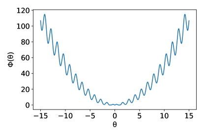
Figure 1: The landscape of the objective function for the illustrative one-dimensional problem.

The convergence histories obtained with these approaches are depicted in Fig. 2. Both Newton and BFGS methods are prone to be trapped in local optima, primarily because only local gradient and Hessian information are used in the solution process. However, neither ETKI nor UKI are trapped in local optima. For UKI, although there is no guarantee that the global minimizer can be found, the ensemble $\{\theta_{n+1}^{j}\}$ around the mean value $\widehat{m}_{n+1}$ brings non-local information and has averaging effect ⁷⁵ on the landscape. And therefore, it is able to avoid local optima. Compared to UKI, ETKI suffers from random noise, and the estimated means oscillate around the optima.

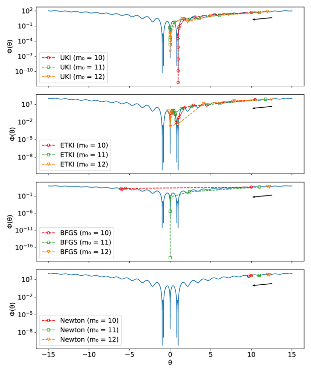
Figure 2: Convergence histories of different optimization approaches initialized at $m_{0}=10$ (red circle dashed lines), $m_{0}=11$ (green square dashed lines), and $m_{0}=12$ (orange triangle dashed lines) for the illustrative one-dimensional problem.

3 Fluid Structure Interaction under Embedded Boundary Framework

3.1 Governing Equations

We consider solving fluid-structure interaction problems involving large structural deformations and even structural damage. Let $\Omega_{F}$ and $\Omega_{S}$ denote the fluid and the structural subdomains. The fluid is assumed to be compressible and inviscid, governed by the following Euler equations in the Eulerian frame

$$\frac{\partial W(x,t)}{\partial t}+\nabla\cdot\mathcal{F}(W)=0,\qquad\forall x\in\Omega_{F}(t),\,t>0,$$ (14)

$$W=\begin{bmatrix}\rho\\ \rho v\\ \rho e_{t}\end{bmatrix},\qquad\mathcal{F}=\begin{bmatrix}\rho v^{T}\\ \rho v\otimes v+p\mathds{I}\\ (\rho e_{t}+p)v^{T}\end{bmatrix},$$

where $\rho$, $v$, $p$ and $e_{t}$ denote the fluid density, velocity, pressure, and the total energy per unit mass, respectively. $\mathds{I}$ denotes an identity matrix. The fluid is assumed to be a perfect gas, and the following equation of state is applied to close Eq. 14

$$p=\left(\gamma_{G}-1\right)\rho e,$$ (15)

where the heat capacity ratio $\gamma_{G}$ is set to be $1.4$ in this work, and $e$ denotes the internal energy per unit mass.

The dynamics of structure is governed by the following equation of motion in the Lagrangian frame

$$\rho_{s}\ddot{u}(X,t)-\nabla\cdot\sigma=b,\qquad\forall X\in\Omega_{S}(0),\,t>0,$$ (16)

where $u$ denotes displacement, $\rho_{s}$ the material’s mass density and $\sigma$ the Cauchy or Piola-Kirchhoff stress tensor. $b$ denotes the body force acting in $\Omega_{S}$, which is assumed to be zero in this study. The dot above a variable represents partial derivative with respect to time. Given a structural material of interest, the closure of (16) is performed by specifying a constitutive law that relates the stress tensor $\sigma$ to the strain tensor $\epsilon$.

The fluid-structure interface, $\Gamma_{FS}=\partial\Omega_{F}(t)\cap\partial\Omega_{S}(t)$, is assumed to be impermeable, at which we enforce the continuity of normal velocity and surface traction, i.e.,

$$\begin{split}(v-\dot{u})\cdot n=0,\qquad&\text{on}\quad\Gamma_{FS},\\ -pn=\sigma\cdot n,\qquad&\text{on}\quad\Gamma_{FS},\end{split}$$ (17)

where $n$ denotes the unit normal to $\Gamma_{FS}$.

3.2 An Embedded Boundary Computational Framework

The above coupled problem is solved by a recently developed fluid-structure coupled computational framework^{95, 18, 96, 21, 97}—AERO-Suite . The framework couples a finite volume CFD solver with a finite element computational structural dynamics solver using an embedded boundary method and a partitioned coupling procedure. The framework has been verified and validated on various applications, including dynamic implosion of underwater cylindrical shells ^{18, 96, 98}, F/A-18 vertical tail buffeting ²⁰, and Mars landing parachute inflation dynamics ^{99, 5, 100}.

3.2.1 FIVER: A Finite Volume Method Based on Exact Riemann Solver

The fluid governing equation is semi-discretized in an augmented fluid domain $\widetilde{\Omega}=\Omega_{F}\cup\Omega_{S}$, using an unstructured, node centered, non-interface-conforming finite volume mesh, denoted by $\widetilde{\Omega}^{h}$. Figure 3 presents an example to illustrate the non-interface-conforming mesh. Within each control volume ($\mathcal{C}_{i}$) in $\widetilde{\Omega}^{h}$, Eq. 14 is integrated as

$$\frac{\partial W_{i}}{\partial t}+\frac{1}{\lVert\mathcal{C}_{i}\rVert}\sum\limits_{j\in Nei(i)}\int_{\partial\mathcal{C}_{ij}}\mathcal{F}(W)\cdot n_{ij}dS=0,$$ (18)

where $W_{i}$ denotes the average of $W$ in $\mathcal{C}_{i}$, $\lVert\mathcal{C}_{i}\rVert$ denotes the volume of $\mathcal{C}_{i}$, $Nei(i)$ denotes the set of nodes connected to node $i$ by an edge, $\partial\mathcal{C}_{ij}=\partial\mathcal{C}_{i}\cap\partial\mathcal{C}_{j}$, and $n_{ij}$ is the unit normal to $\partial\mathcal{C}_{ij}$. Away from the fluid-structure interface, the flux through each segment $\partial\mathcal{\mathcal{C}}_{ij}$ in Eq. 18 is approximated using Roe’s (or any other similar) approximate Riemann solver ¹⁰¹ equipped with a MUSCL technique ¹⁰² and a slope limiter.

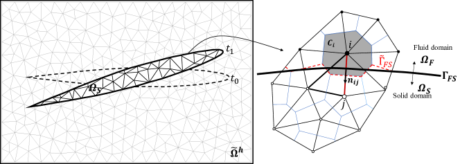
Figure 3: Illustration of the non-interface-conforming mesh under embedded boundary framework.

At the embedded fluid-structure interface, the flux in Eq. 18 is approximated with the reconstructed fluid state vector, which satisfies the transmission conditions (17). The reconstruction is through solving a one-dimensional fluid-solid Riemann problem. Specifically, as shown in the right figure in Figure 3, suppose node $i$ belongs to the fluid subdomain, node $j$ belongs to the solid subdomain, and edge $i$-$j$ intersects the embedded interface $\Gamma_{FS}$. We construct the following one-dimensional fluid-solid Riemann problem along $n_{S}$, the unit normal of $\Gamma_{FS}$ (toward the structure) at its intersection with edge $i$-$j$, at each time-instance $t_{n}$

$$\frac{\partial{w}}{\partial\tau}+\frac{\partial{\mathcal{F}}({w})}{\partial\xi} = 0,\quad\quad 0\leq\tau\leq\Delta t^{n},~{}\xi<(\dot{u}_{0}\cdot n_{S})\tau,$$ (19)

$${w}(\xi,0) = w_{i},\quad\quad\mbox{$\xi<0$,}$$ (20)

$$v((\dot{u}_{0}\cdot n_{S})\tau,\tau) = \dot{u}_{0}\cdot n_{S},\quad\quad 0\leq\tau\leq\Delta t_{n},$$ (21)

$\xi$ is the spatial coordinate along the one-dimensional axis aligned with $n_{S}$ and centered at the intersection point. The initial state $w_{i}$ is the projection of $W_{i}$ on $n_{S}$, i.e.

$$w_{i}=\begin{bmatrix}\rho_{i}\\ \rho_{i}(v_{i}\cdot n_{S})\\ \rho_{i}\big{(}e_{i}+\frac{1}{2}(v_{i}\cdot n_{S})^{2}\big{)}\\ \end{bmatrix}.$$ (22)

$\dot{u}_{0}$ denotes the velocity of the structure at $t_{n}$. The exact solution of this Riemann problem can be derived analytically. And the state variables and the tangential fluid velocity are used to reconstruct the fluid state vector at the fluid-structure interface. The resulting semi-discretization of Eq. 14 can be written in a compact form as

$$\frac{d\mathbf{W}^{h}}{dt}+\mathbf{V}^{-1}\mathbf{F}(\mathbf{W}^{h})=0,$$ (23)

where $\mathbf{W}^{h}$, $\mathbf{V}$, and $\mathbf{F}(\mathbf{W}^{h})$ denote the vector of semidiscrete fluid state variable, the diagonal matrix storing the volume of control volumes, and the vector of numerical flux, respectively.

3.2.2 A Finite Element Structural Solver

The structural governing equation is solved using a standard Galerkin finite element method. The semi-discretized equation is written as

$$\mathbf{M}\frac{\partial^{2}\mathbf{u}^{h}}{\partial t^{2}}+\mathbf{f}^{int}\Big{(}\mathbf{u}^{h},\frac{\partial\mathbf{u}^{h}}{\partial t}\Big{)}=\mathbf{f}^{ext},$$ (24)

where $\mathbf{M}$ denotes the mass matrix, $\mathbf{u}^{h}$ denotes the discrete displacement vector. $\mathbf{f}^{int}$ and $\mathbf{f}^{ext}$denote the discrete internal force and external force vector, respectively. Based on the dynamics interface condition (Eq. 17), the fluid-induced external forces are computed by integrating the fluid pressure over the embedded interface. Additional details can be found in Section 3.8.3 in the work of Main ¹⁰³.

3.2.3 Partitioned Coupling Procedure

We employ a partitioned procedure to advance the fluid subsystem (23) and structure subsystem (24) in time, following the work of Farhat et al. ⁹⁵. Specifically, the fluid and structural discretized equations are solved independently with different time integrators. The two solvers exchange information at the fluid-structure interface once per time step in a staggered manner, i.e., the fluid and solid time steps are offset by half a step. This is a designed feature to achieve second-order accuracy in time while maintaining optimal numerical stability.

4 Numerical Results

In this section, we apply the unscented Kalman inversion and the embedded boundary framework presented in Sections 2 and 3 to calibrate parameters, as well as quantify their uncertainty, for two FSI problems with noisy observation data. The first case is a one-dimensional piston model problem, where the damping coefficient, the spring stiffness, and the initial fluid pressure are calibrated from the piston displacement. The second case is a challenging three-dimensional aeroelasticity problem of a damaged aircraft wing, where the damage field, specifically the coefficients of first 5 modes, is inferred from the displacement during its transonic buffet. For both cases, we prescribe a reference value for the parameters of interest and generate the time-series observation data in which additional Gaussian random noise is added. Then, using the noisy data, we solve the Bayesian calibration problem to retrieve the predefined parameters and associated uncertainties. The code associated with these two test cases is accessible online: https://github.com/Zhengyu-Huang/InverseProblems.jl.

4.1 Piston Problem

We first consider a canonical FSI model problem: a one-dimensional piston problem depicted in Fig. 4. The inviscid fluid is governed by the one-dimensional Euler equations defined within domain $x\in[0,1-u]$, where $u$ is the displacement of the piston. The fluid is initially at rest, with initial density, velocity, and pressure given by:

$$\rho_{0}=1.225,\qquad v_{0}=0,\qquad p_{0}=2.0.$$

No-penetration wall boundary condition is imposed on the left end of the fluid domain. On the right, the fluid interacts with a piston. The piston is connected with a spring and a damper that are attached to a wall on the right at $x=1$. The dynamics of the piston can be described by the second order ordinary differential equation:

$$m_{s}\ddot{u}+c_{s}\dot{u}+k_{s}{u}=f^{ext},$$

where the mass coefficient is $m_{s}=1$, the damping coefficient is $c_{s}=0.5$, and the spring stiffness is $k_{s}=2$. The external force $f_{ext}$ is the fluid pressure load on the piston:

$$f^{ext}(t)=p(x_{p}(t)),$$

where $x_{p}(t)=1-u(t)$. The piston is initialized at $x=1$, with $u(0)=0$ and $\dot{u}(0)=0$.

Figure 4: One-dimensional piston system

For the forward problem, the computational domain is semi-discretized by a uniform grid with $\Delta x=5\times 10^{-3}$. The explicit 2nd-order Runge-Kutta time integrator  is used for the fluid and implicit 2nd-order mid-point rule time integrator is applied for the structure with a constant time step $\Delta t=10^{-3}$. The coupling between fluid and structure is based on a partitioned procedure and an embedded boundary method which are applied in FIVER (Section 3.2). The coupled system is integrated till the final time $T=1$.

For the inverse problem, we consider two scenarios:

1. calibrate only the structure parameters $\theta=[c_{s};\,k_{s}]$ with $N_{\theta}=2$;

2. calibrate both structure parameters and fluid initial pressure $\theta=[c_{s};\,k_{s};\,p_{0}]$ with $N_{\theta}=3$.

The observation data consist of $N_{y}=100$ piston displacement measurements collected at every $10^{-2}$ till $T=1$. These observation data are generated with reference parameters and corrupted with zero-mean random Gaussian noise with standard deviation $\sigma_{\eta}=2\times 10^{-3}$. The observation data are depicted in Fig. 5-left; and the corresponding fluid states at the end time is depicted in Fig. 5-right , the rarefaction wave is generated in the flow due to the receding motion of the piston.

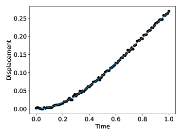
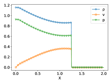
Figure 5: Left: the displacement of the piston with $100$ noisy measurements (black dots); Right: the fluid states at the end time.

For both scenarios, the UKI is initialized with $\theta_{0}\sim\mathcal{N}(\mathds{1},0.1^{2}\mathds{I})$. The estimated parameters and associated 2-$\sigma$ confidence intervals for each component at each iteration are depicted in Fig. 6. The UKI converges efficiently. Reference values falls within the confidence interval with high probability, although the uncertainty is larger for the 3-parameter scenario.

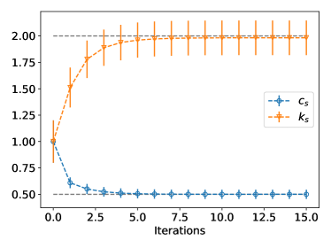
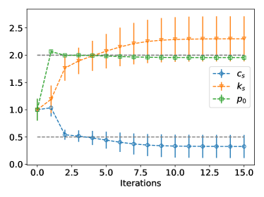
Figure 6: Convergence of the piston model problem with UKI for both 2-parameter (left) and 3-parameter (left) scenarios; the true parameter values are represented by dashed grey lines. The error bar associated with each data point denotes the $2-\sigma$ confidence intervals.

The reference posterior distribution is approximated by the random walk MCMC method with a step size $1.0\times 10^{-2}$ and $5\times 10^{4}$ samples (with a $10^{4}$ sample burn-in period). The posterior distributions obtained by the UKI at the 15th iteration are depicted in Fig. 7. The UKI delivers a very similar posterior distribution, but at a significantly cheaper computational cost.

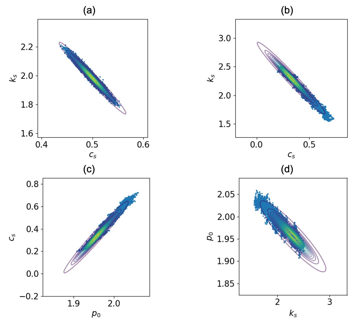
Figure 7: Pairwise posterior distribution of the piston model problem for both 2-parameter (a) and 3-parameter (b-d) scenarios. Contour plot: the posterior distribution obtained by the UKI at the 15th iteration; blue dots: reference posterior distribution obtained by MCMC.

4.2 Wing Damage Detection Problem

The second test is a challenging real-world FSI problem associated with a damaged AGARD wing ¹⁰⁴ undergoing transonic buffet. We consider a cruise condition, where the atmospheric density is $\rho_{\infty}=0.61\times 10^{-7}~{}\textrm{slug/in}^{3}$ and the atmospheric pressure is $p_{\infty}=6~{}\textrm{slugs}/(\textrm{in}\cdot\textrm{s}^{2})$; the free-stream Mach number is $M_{\infty}=0.97$; and the angle of attack is $\alpha=7.5^{\circ}$. The AGARD wing structure is modeled as a nonlinear elastic composite shell (See Fig. 8-left). The orthotropic properties of this material are density $\rho_{s}=4.6\times 10^{-4}~{}\textrm{slug/in}^{3}$, parallel Young’s modulus $E_{1}=5.874\times 10^{6}~{}\textrm{slug}/(\textrm{in}\cdot\textrm{s}^{2})$, orthogonal Young’s modulus $E_{2}=7.20\times 10^{6}~{}\textrm{slug}/(\textrm{in}\cdot\textrm{s}^{2})$, rigidity modulus $G=7.1688\times 10^{5}\textrm{slug}/(\textrm{in}\cdot\textrm{s}^{2})$, and Poisson’s ratio $\nu=0.31$. The physical dimensions are reported in Table 1. The thickness distribution is governed by the airfoil shape.

Table 1: Geometrical properties of the AGARD wing.

Parameter	Type/Value
Wingspan	30 inches
Root chord	21.96 inches
Tip chord	14.5 inches
Sweep	45∘

The computational fluid domain $[-100^{\prime\prime},\,150^{\prime\prime}]\times[0^{\prime\prime},\,150^{\prime\prime}]\times[-100^{\prime\prime},\,100^{\prime\prime}]$ is discretized by the three-dimensional tetrahedral Eulerian mesh. The mesh contains $218,880$ vertices and $1,248,912$ tetrahedral elements, with a $0.75$ inch resolution near the AGARD wing (See Fig. 8-right). The AGARD wing finite element model ¹⁰⁵ consists of $800$ triangular composite shell elements and $2,646$ degrees of freedom (See Fig. 8-left-top). The embedded surface, representing the wing skin surface, consists of 2788 triangles (See Fig. 8-left-bottom).

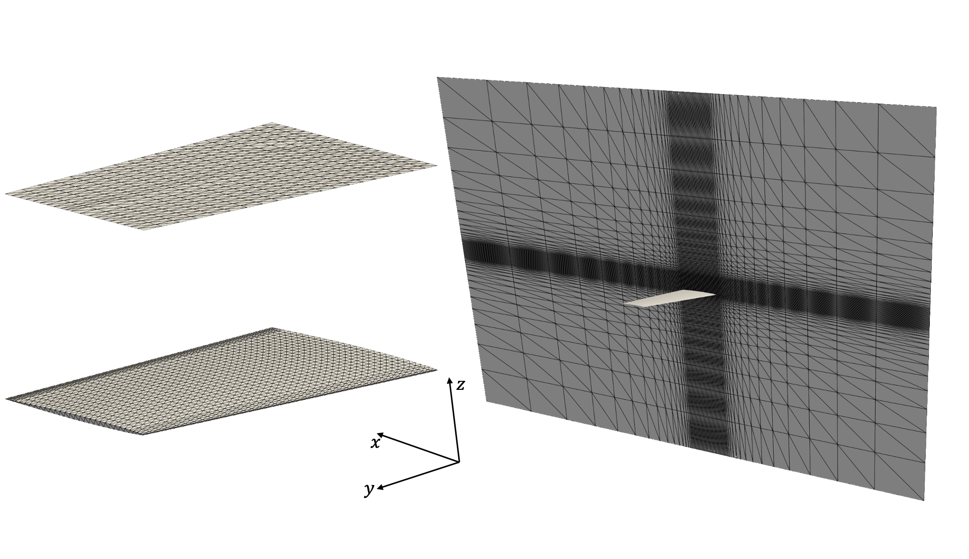
Figure 8: Computational models for the AGARD wing: finite element structural model (left-top), the wing skin surface of this model (left-bottom), and CFD mesh (right).

We assume the damage in aircraft wing to be isotropic elasticity-based damage and consider only the damage in the spar direction ($y$-direction) for simplicity. Specifically, a simple continuum damage model is used in which a scalar damage variable $\omega$ is used to measure the average damage effects on the material’s mechanical response. The damage effects are imposed by modifying the elastic moduli of the material:

$$E_{1}^{d}(y,\theta)=\left(1-\omega(y,\theta)\right)E_{1}\qquad E_{2}^{d}(y,\theta)=\left(1-\omega(y,\theta)\right)E_{2}\qquad\textrm{and}\qquad G^{d}(y,\theta)=\left(1-\omega(y,\theta)\right)G.$$

Here, the damage $\omega(y,\theta)$ is designed to vary between $\omega_{min}=-0.1$ (hardening) to $\omega_{max}=0.9$ (softening):

$$\omega(y,\theta)=\frac{\omega_{max}-\omega_{min}}{1-\frac{\omega_{max}}{\omega_{min}}\exp\left(\log a(y,\theta)\right)}+\omega_{min},$$ (25)

where $\log a(y,\theta)$ is a log-Gaussian random field that depends on parameters $\theta\in\mathbb{R}^{N_{\theta}}$. Specifically, the log-Gaussian random field is approximated by the following Karhunen-Loève (KL) expansion

$$\log a(y,\theta)=\sum_{l=1}^{+\infty}\theta_{(l)}\sqrt{\lambda_{l}}\psi_{l}(y),$$ (26)

where the random variables $\theta_{(l)}\sim\mathcal{N}(0,1)$ are independent and identically distributed, and the eigenpairs are of the form

$$\psi_{l}(y)=\sqrt{2}\cos(\pi ly)\quad\textrm{ and }\quad\lambda_{l}=(\pi^{2}l^{2}+\tau^{2})^{-d}\quad\text{with}\quad\tau=2,\quad d=1.$$

This setup gives rise to a zero mean state of $\log a(y,\theta)$ which corresponds to the undamaged state $\omega(y,\theta)=0$. And the damage $\omega$ increases monotonically with $\log a$. In this test, we consider the first 10 KL modes (i.e., with 10 sampled $\theta_{(l)}$) and generate the reference damage field $\omega_{ref}(y)$ from Eqs. 25 and 26. The resulting damage field $\omega_{ref}(y)$ is depicted in Fig. 11.

For the forward problem, we apply FIVER (Section 3.2) to solve for the fluid dynamics and structural response. Specifically, an implicit backward Euler time integrator is used for the fluid and an implicit 2nd order mid-point rule time integrator is applied to for the structure with a constant time step $\Delta t=5\times 10^{-5}s$. The simulation starts from a steady flow field depicted in Fig. 9, in which a shock wave forms on the wing. When the coupled simulation starts, the wing starts buffeting, interacts with the shock wave, and undergoes large deformations (See Fig. 10). The coupled system is integrated till $T=0.1s$. And each forward run takes about 36 core hours.

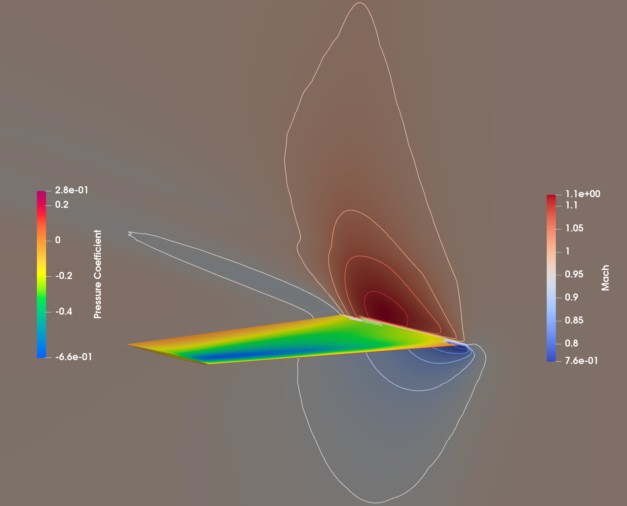
Figure 9: Initial condition for the FSI simulation: pressure coefficient on the wing and Mach contour profile in the fluid. The initial condition is also the converged steady state result with a fixed AGARD wing.

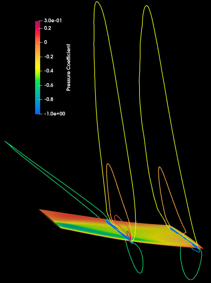
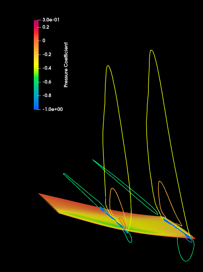
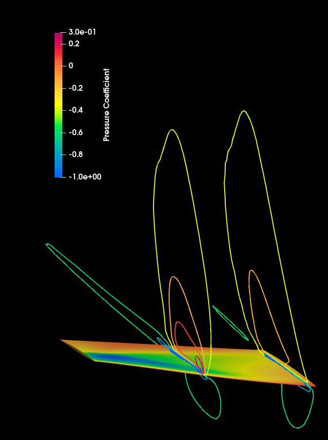
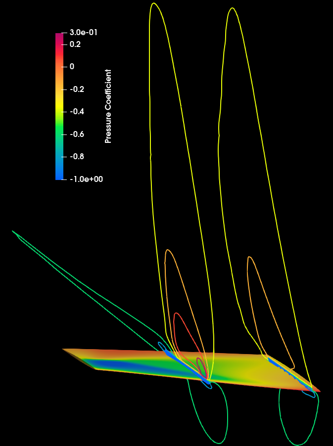
Figure 10: AGARD wing transonic buffeting: Snapshots of the fluid-structure solution at t = 0.025 s, t = 0.05 s, t = 0.075 s, t = 0.10 s (left to right) with pressure coefficient on the wing and Mach contour in the fluid.

For the inverse problem, the damage field $\omega(y,\theta)$ is inferred from the displacement measurements of the wing buffeting motion. With the reference damage field, we construct the observation $y_{obs}$ at 12 locations (See Fig. 11) on the leading edge, half chord position, and trailing edge with $5\%$ synthetic Gaussian random noises:

$$y_{obs}=y_{ref}+5\%y_{ref}\odot\mathcal{N}(0,\mathds{I}),$$

where $\odot$ denotes element-wise multiplication. The observation data are collected every $0.002$ s, giving $N_{y}=600$ observation data in total (See Fig. 14).

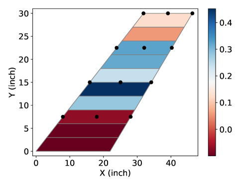
Figure 11: Reference damage field $\omega_{ref}(y)$ of the AGARD wing and the 12 pointwise measurement locations (black dots).

The UKI is applied to retrieve the first $N_{\theta}=5$ KL modes; in essence the model form error exists. The solution process is initialized with $m_{0}=0$ (no damage) and $C_{0}=\mathds{I}$, and hence $\theta_{0}\sim\mathcal{N}(0,\mathds{I})$. The observation error is set to follow $\eta\sim\mathcal{N}(0,0.1^{2}\mathds{I})$; in essence we assume imperfect knowledge of the noise model. For $N_{\theta}=5$, each iteration includes $11$ parallel forward runs. The optimization errors $\Phi(\theta)$ in Eq. 3 at each iteration are plotted in Fig. 12, showing fast convergence. The estimated damage field $\omega(y,\theta)$ and the associated 2-$\sigma$ confidence intervals at the $15$-th iteration are depicted in Fig. 13. The truth damage field $\omega_{ref}$ falls within the confidence interval with high probability. The predicted displacement fields at these measurement locations and the displacement predicted with the initial guess (no-damage case) are depicted in Fig. 14. It is worth mentioning that all displacement curves are very close to the observation data, which indicates the wing displacement is not very sensitive to the damage. However, UKI still delivers a good estimate of the damage field, which demonstrates the effectiveness of the Bayesian calibration procedure for real-world applications.

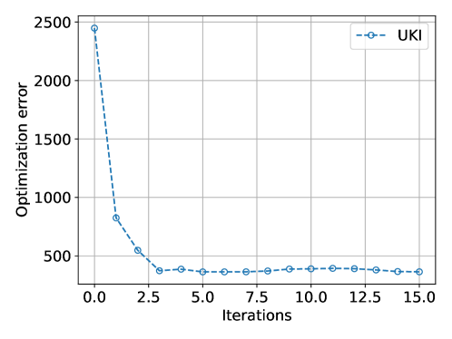
Figure 12: The optimization error $\frac{1}{2}\lVert\Sigma_{\eta}^{-\frac{1}{2}}(y-\mathcal{G}(\theta))\rVert^{2}$ at each UKI iteration for the wing damage detection problem.

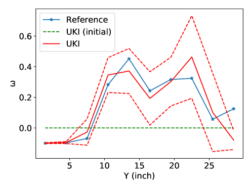
Figure 13: The estimated damage field $\omega(y,\theta_{n})$ (red solid line) and the associated 2-$\sigma$ confidence intervals (red dashed lines) at the $15$-th iteration; The reference damage field $\omega_{r}ef(y)$ (blue star line); The initial guess of the damage field at the $0$-th iteration (green dashed line) for the wing damage detection problem.

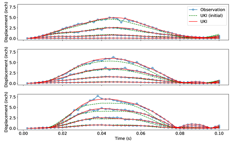
Figure 14: Blue dot lines: displacement observation data on the leading edge measurement locations (top), on the half-chord measurement locations (middle), on the trailing edge measurement locations (bottom) with the damaged AGARD wing. Dashed green lines: predictions with the initial guess (no damage). Red lines: predictions with the damage field obtained by the UKI at the 15th iteration.

5 Conclusion

This paper presents a general Bayesian calibration framework for FSI problems based on unscented Kalman inversion. It is attractive for at least four reasons: i) It is non-intrusive and derivative-free; ii) It is robust for chaotic inverse problems with noisy observations; iii) It provides uncertainty information; iv) It is embarrassingly parallel. It is well-adapted to parameter/field estimation problems for any large complex computational models given as a black box. There are numerous directions for future improvements:

• At each iteration, UKI requires solving the forward problem $2N_{\theta}+1$ times. Although these forward solver evaluations are embarrassingly parallel, the computational cost might be intractable when the number of parameters $N_{\theta}$ is large or the forward evaluation is expensive. The use of reduced-order models, including but not limit to neural network surrogate models ^{106, 107, 108, 109, 110}, projection-based reduced order models ^{111, 112, 113, 114, 115}, and Kernel-based surrogate models ^{116, 117, 118}, is worth exploring in the future.

• For the damage detection problem in Subsection 4.2, the sensors are uniformly located on the aircraft wing. Optimal sensor placement ^{119, 120, 121}, which potentially makes data collection more efficient and makes the algorithm converge faster, is worth further investigation. And more realistic damage and fracture models ^{122, 123, 124} will be considered in the future.

• For Bayesian calibration problems with time-series data studied in the present work, other Kalman methodology (e.g. Kalman smoother ^{125, 126, 127}) will be applied and studied in the future.

6 acknowledgement*

The authors gratefully acknowledge the support of National Institutes of Health under Award P01-DK043881 and the generosity of Eric and Wendy Schmidt by recommendation of the Schmidt Futures program. The authors thank Dr. Kevin G. Wang and Dr. Fangbao Tian for their advice on the manuscript.

7 data availability statement*

All computer code used in this paper is open source. Datasets, including mesh files and results, are available at https://github.com/Zhengyu-Huang/InverseProblems.jl.

Appendix A Proof of Theorem 2.2

Thanks to the linearity, the Eqs. (7) are reduced to

$$\widehat{y}_{n+1}=Gm_{n},\quad\widehat{C}_{n+1}^{\theta p}=\widehat{C}_{n+1}G^{T},\quad\textrm{and}\quad\widehat{C}_{n+1}^{pp}=G\widehat{C}_{n+1}G^{T}+\Sigma_{\nu}.$$

The update equations (8) become

$$\begin{split}m_{n+1}&=m_{n}+\widehat{C}_{n+1}G^{T}(G\widehat{C}_{n+1}G^{T}+\Sigma_{\nu})^{-1}(y-Gm_{n}),\\ C_{n+1}&=\widehat{C}_{n+1}-\widehat{C}_{n+1}G^{T}(G\widehat{C}_{n+1}G^{T}+\Sigma_{\nu})^{-1}G\widehat{C}_{n+1},\end{split}$$ (27)

with $\widehat{C}_{n+1}=C_{n}+\Sigma_{\omega}$.

With the hyperparameters defined in Eq. 11, the update equation of $\{C_{n}\}$ in Eq. 27 can be rewritten as

$$\begin{split}&C_{n+1}^{-1}=G^{T}\Sigma_{\nu}^{-1}G+(C_{n}+\Sigma_{\omega})^{-1}=\frac{1}{2}G^{T}\Sigma_{\eta}^{-1}G+(2C_{n})^{-1}.\\ \end{split}$$ (28)

We have a closed formula for $C^{-1}_{n}$:

$$C_{n}^{-1}=\Big{[}1-\frac{1}{2^{n}}\Big{]}G^{T}\Sigma_{\eta}^{-1}G+\frac{1}{2^{n}}C_{0}^{-1}.$$ (29)

This leads to the exponential convergence $\displaystyle\lim_{n\to\infty}C_{n}^{-1}=G^{T}\Sigma_{\eta}^{-1}G$.

The convergence proof of $m_{n}$ basically follows the work of Huang et al. ⁷⁵. Equations 28 and 29 lead to

$$\begin{split}\frac{1}{2}G^{T}\Sigma_{\eta}^{-1}G=G^{T}\Sigma_{\nu}^{-1}G\preceq C_{n+1}^{-1}\preceq G^{T}\Sigma_{\nu}^{-1}G+\Sigma_{+}\quad\textrm{where}\quad\Sigma_{+}=G^{T}\Sigma_{\nu}^{-1}G+C_{0}^{-1}.\end{split}$$ (30)

The update equation of $m_{n}$ in Eq. 27 can be rewritten as

$$m_{n+1}=m_{n}+C_{n+1}G^{T}\Sigma_{\nu}^{-1}(y-Gm_{n}).$$ (31)

We have the assumption that $G$ has full column rank, and therefore, $B:=G^{T}\Sigma_{\nu}^{-1}G$ is positive definite. From this, it follows that $\mathds{I}-C_{n+1}B$ has the same spectrum as $\mathds{I}-B^{\frac{1}{2}}C_{n+1}B^{\frac{1}{2}}$. Using the bounds on $C_{n+1}$ appearing in Eq. 30, the spectral radius of the update matrix in Eq. 31 satisfies

$$\begin{split}\rho(\mathds{I}-C_{n+1}G^{T}\Sigma_{\nu}^{-1}G)&=\rho(\mathds{I}-C_{n+1}B)\\ &=\rho\Big{(}\mathds{I}-\sqrt{B}C_{n+1}\sqrt{B}\Big{)}\\ &\leq 1-\rho\Big{(}\sqrt{B}\big{(}B+\Sigma_{+}\big{)}^{-1}\sqrt{B}\Big{)}\\ &=1-\epsilon_{0},\end{split}$$ (32)

where $\epsilon_{0}\in(0,1)$. Hence, we have that $\{m_{n}\}$ converges exponentially to $m_{\infty}$, which satisfies $\displaystyle G^{T}\Sigma_{\nu}^{-1}(y-Gm_{\infty})=0$. And it is a minimizer of $\Phi$.

As for the uncertainty estimation, we have

$$G^{T}\Sigma_{\eta}^{-1}(y-Gm_{\infty})=0\qquad C^{-1}_{\infty}=G^{T}\Sigma_{\eta}^{-1}G.$$

and

$$\eta_{r}=y-G\theta_{ref}\sim\mathcal{N}(0,\Sigma_{\eta}).$$

When $G$ is of full column rank, $G^{T}\Sigma_{\eta}^{-1}G$ is non-singular. We have

$$\begin{split}&\theta_{ref}-m_{\infty}=-\Big{(}G^{T}\Sigma_{\eta}^{-1}G\Big{)}^{-1}G^{T}\Sigma_{\eta}^{-1}\eta_{r},\\ &\theta_{ref}-m_{\infty}\sim\mathcal{N}\Big{(}0,\big{(}G^{T}\Sigma_{\eta}^{-1}G\big{)}^{-1}\Big{)}=\mathcal{N}(0,C_{\infty}).\end{split}$$

Therefore, each component of $\theta_{ref}-m_{\infty}$ obeys Gaussian distribution,

$${\theta_{ref}}_{(i)}-{m_{\infty}}_{(i)}\sim\mathcal{N}(0,{C_{\infty}}_{(i,i)}).$$

The empirical rule of Gaussian implies Equation 13.

References

- 1 Geuzaine P, Brown G, Harris C, Farhat C. Aeroelastic dynamic analysis of a full F-16 configuration for various flight conditions. AIAA journal 2003; 41(3): 363–371.
- 2 Kamakoti R, Shyy W. Fluid–structure interaction for aeroelastic applications. Progress in Aerospace Sciences 2004; 40(8): 535–558.
- 3 Dowell E. Some recent advances in nonlinear aeroelasticity: fluid-structure interaction in the 21st century. In: AIAA. ; 2010: 3137.
- 4 Huang Z, Avery P, Farhat C, Rabinovitch J, Derkevorkian A, Peterson LD. Simulation of parachute inflation dynamics using an Eulerian computational framework for fluid-structure interfaces evolving in high-speed turbulent flows. In: AIAA. ; 2018: 1540.
- 5 Huang DZ, Avery P, Farhat C, Rabinovitch J, Derkevorkian A, Peterson LD. Modeling, simulation and validation of supersonic parachute inflation dynamics during Mars landing. In: AIAA. ; 2020: 0313.
- 6 Avery P, Huang DZ, He W, Ehlers J, Derkevorkian A, Farhat C. A computationally tractable framework for nonlinear dynamic multiscale modeling of membrane woven fabrics. International Journal for Numerical Methods in Engineering 2021.
- 7 Hsu MC, Kamensky D, Bazilevs Y, Sacks MS, Hughes TJ. Fluid–structure interaction analysis of bioprosthetic heart valves: significance of arterial wall deformation. Computational mechanics 2014; 54(4): 1055–1071.
- 8 Updegrove A, Wilson NM, Merkow J, Lan H, Marsden AL, Shadden SC. SimVascular: an open source pipeline for cardiovascular simulation. Annals of biomedical engineering 2017; 45(3): 525–541.
- 9 Bertaglia G, Caleffi V, Pareschi L, Valiani A. Uncertainty quantification of viscoelastic parameters in arterial hemodynamics with the a-FSI blood flow model. Journal of Computational Physics 2021; 430: 110102.
- 10 Cao S, Zhang Y, Liao D, Zhong P, Wang KG. Shock-induced damage and dynamic fracture in cylindrical bodies submerged in liquid. International journal of solids and structures 2019; 169: 55–71.
- 11 Cao S, Wang G, Coutier-Delgosha O, Wang K. Shock-induced bubble collapse near solid materials: effect of acoustic impedance. Journal of Fluid Mechanics 2021; 907.
- 12 Ismail M, Wall WA, Gee MW. Adjoint-based inverse analysis of windkessel parameters for patient-specific vascular models. Journal of Computational Physics 2013; 244: 113–130.
- 13 Arthurs CJ, Xiao N, Moireau P, Schaeffter T, Figueroa CA. A flexible framework for sequential estimation of model parameters in computational hemodynamics. Advanced modeling and simulation in engineering sciences 2020; 7(1): 1–37.
- 14 Sohn H, Law KH. A Bayesian probabilistic approach for structure damage detection. Earthquake engineering & structural dynamics 1997; 26(12): 1259–1281.
- 15 Tuegel EJ, Ingraffea AR, Eason TG, Spottswood SM. Reengineering aircraft structural life prediction using a digital twin. International Journal of Aerospace Engineering 2011; 2011.
- 16 Sotoudehnia E, Shahabian F, Sani AA. A new method for damage detection of fluid-structure systems based on model updating strategy and incomplete modal data. Ocean Engineering 2019; 187: 106200.
- 17 Löhner R, Baum JD, Mestreau E, Sharov D, Charman C, Pelessone D. Adaptive embedded unstructured grid methods. International Journal for Numerical Methods in Engineering 2004; 60(3): 641–660.
- 18 Wang K, Rallu A, Gerbeau JF, Farhat C. Algorithms for interface treatment and load computation in embedded boundary methods for fluid and fluid–structure interaction problems. International Journal for Numerical Methods in Fluids 2011; 67(9): 1175–1206. doi: 10.1002/fld.2556
- 19 Farhat C, Gerbeau JF, Rallu A. FIVER: A finite volume method based on exact two-phase Riemann problems and sparse grids for multi-material flows with large density jumps. Journal of Computational Physics 2012; 231(19): 6360–6379. doi: https://doi.org/10.1016/j.jcp.2012.05.026
- 20 Lakshminarayan V, Farhat C, Main A. An embedded boundary framework for compressible turbulent flow and fluid–structure computations on structured and unstructured grids. International Journal for Numerical Methods in Fluids 2014; 76(6): 366–395. doi: 10.1002/fld.3937
- 21 Main A, Zeng X, Avery P, Farhat C. An enhanced FIVER method for multi-material flow problems with second-order convergence rate. Journal of Computational Physics 2017; 329: 141–172. doi: https://doi.org/10.1016/j.jcp.2016.10.028
- 22 Peskin CS. Flow patterns around heart valves: A numerical method. Journal of Computational Physics 1972; 10(2): 252–271. doi: https://doi.org/10.1016/0021-9991(72)90065-4
- 23 Fadlun E, Verzicco R, Orlandi P, Mohd-Yusof J. Combined immersed-boundary finite-difference methods for three-dimensional complex flow simulations. Journal of Computational Physics 2000; 161(1): 35–60. doi: https://doi.org/10.1006/jcph.2000.6484
- 24 Kim J, Kim D, Choi H. An immersed-boundary finite-volume method for simulations of flow in complex geometries. Journal of Computational Physics 2001; 171(1): 132–150. doi: https://doi.org/10.1006/jcph.2001.6778
- 25 Uhlmann M. An immersed boundary method with direct forcing for the simulation of particulate flows. Journal of Computational Physics 2005; 209(2): 448–476.
- 26 Choi JI, Oberoi RC, Edwards JR, Rosati JA. An immersed boundary method for complex incompressible flows. Journal of Computational Physics 2007; 224(2): 757–784. doi: https://doi.org/10.1016/j.jcp.2006.10.032
- 27 Taira K, Colonius T. The immersed boundary method: a projection approach. Journal of Computational Physics 2007; 225(2): 2118–2137.
- 28 Tian FB, Dai H, Luo H, Doyle JF, Rousseau B. Fluid–structure interaction involving large deformations: 3D simulations and applications to biological systems. Journal of computational physics 2014; 258: 451–469.
- 29 Ingram DM, Causon DM, Mingham CG. Developments in Cartesian cut cell methods. Mathematics and Computers in Simulation 2003; 61(3): 561–572. doi: https://doi.org/10.1016/S0378-4754(02)00107-6
- 30 Schott B, Ager C, Wall WA. Monolithic cut finite element–based approaches for fluid-structure interaction. International Journal for Numerical Methods in Engineering 2019.
- 31 Berger M, Aftosmis M. Progress towards a Cartesian cut-cell method for viscous compressible flow. In: AIAA. ; 2012: 1301.
- 32 Johansen H, Colella P. A Cartesian grid embedded boundary method for Poisson’s equation on irregular domains. Journal of Computational Physics 1998; 147(1): 60–85. doi: https://doi.org/10.1006/jcph.1998.5965
- 33 Uddin H, Kramer R, Pantano C. A Cartesian-based embedded geometry technique with adaptive high-order finite differences for compressible flow around complex geometries. Journal of Computational Physics 2014; 262: 379–407. doi: 10.1016/j.jcp.2014.01.004
- 34 Harris RE. Adaptive Cartesian immersed boundary method for simulation of flow over flexible geometries. AIAA Journal 2012; 51(1): 53–69. doi: 10.1006/jcph.1999.6293
- 35 Almgren AS, Bell JB, Colella P, Marthaler T. A Cartesian grid projection method for the incompressible Euler equations in complex geometries. SIAM Journal on Scientific Computing 1997; 18(5): 1289–1309. doi: 10.1137/S1064827594273730
- 36 Balaras E. Modeling complex boundaries using an external force field on fixed Cartesian grids in large-eddy simulations. Computers & Fluids 2004; 33(3): 375–404. doi: https://doi.org/10.1016/S0045-7930(03)00058-6
- 37 Tseng YH, Ferziger JH. A ghost-cell immersed boundary method for flow in complex geometry. Journal of computational physics 2003; 192(2): 593–623. doi: https://doi.org/10.1016/j.jcp.2003.07.024
- 38 Feng ZG, Michaelides EE. The immersed boundary-lattice Boltzmann method for solving fluid–particles interaction problems. Journal of computational physics 2004; 195(2): 602–628.
- 39 Tian FB, Luo H, Zhu L, Liao JC, Lu XY. An efficient immersed boundary-lattice Boltzmann method for the hydrodynamic interaction of elastic filaments. Journal of computational physics 2011; 230(19): 7266–7283.
- 40 Yang X, Zhang X, Li Z, He GW. A smoothing technique for discrete delta functions with application to immersed boundary method in moving boundary simulations. Journal of Computational Physics 2009; 228(20): 7821–7836.
- 41 Goza A, Liska S, Morley B, Colonius T. Accurate computation of surface stresses and forces with immersed boundary methods. Journal of Computational Physics 2016; 321: 860–873.
- 42 Ho J, Farhat C. Discrete embedded boundary method with smooth dependence on the evolution of a fluid-structure interface. International Journal for Numerical Methods in Engineering 2020.
- 43 Ho JB, Farhat C. Aerodynamic Shape Optimization using an Embedded Boundary Method with Smoothness Guarantees. In: AIAA. ; 2021: 0280.
- 44 Berger MJ, Colella P, others . Local adaptive mesh refinement for shock hydrodynamics. Journal of computational Physics 1989; 82(1): 64–84.
- 45 Griffith BE, Hornung RD, McQueen DM, Peskin CS. An adaptive, formally second order accurate version of the immersed boundary method. Journal of computational physics 2007; 223(1): 10–49.
- 46 Borker R, Huang D, Grimberg S, Farhat C, Avery P, Rabinovitch J. Mesh adaptation framework for embedded boundary methods for computational fluid dynamics and fluid-structure interaction. International Journal for Numerical Methods in Fluids 2019; 90(8): 389–424.
- 47 Hirt CW, Amsden AA, Cook J. An arbitrary Lagrangian-Eulerian computing method for all flow speeds. Journal of computational physics 1974; 14(3): 227–253.
- 48 Tezduyar TE, Behr M, Mittal S, Liou J. A new strategy for finite element computations involving moving boundaries and interfaces—the deforming-spatial-domain/space-time procedure: II. Computation of free-surface flows, two-liquid flows, and flows with drifting cylinders. Computer methods in applied mechanics and engineering 1992; 94(3): 353–371.
- 49 Felippa CA, Park KC, Farhat C. Partitioned analysis of coupled mechanical systems. Computer methods in applied mechanics and engineering 2001; 190(24-25): 3247–3270.
- 50 Küttler U, Wall WA. Fixed-point fluid–structure interaction solvers with dynamic relaxation. Computational mechanics 2008; 43(1): 61–72.
- 51 Huang DZ, Persson PO, Zahr MJ. High-order, linearly stable, partitioned solvers for general multiphysics problems based on implicit–explicit Runge–Kutta schemes. Computer Methods in Applied Mechanics and Engineering 2019; 346: 674–706.
- 52 Huang DZ, Pazner W, Persson PO, Zahr MJ. High-order partitioned spectral deferred correction solvers for multiphysics problems. Journal of Computational Physics 2020: 109441.
- 53 Huang DZ, Zahr MJ, Persson PO. A high-order partitioned solver for general multiphysics problems and its applications in optimization. In: AIAA. ; 2019: 1697.
- 54 Dukowicz JK, Kodis JW. Accurate conservative remapping (rezoning) for arbitrary Lagrangian-Eulerian computations. SIAM Journal on Scientific and Statistical Computing 1987; 8(3): 305–321.
- 55 Long C, Marsden A, Bazilevs Y. Fluid–structure interaction simulation of pulsatile ventricular assist devices. Computational Mechanics 2013; 52(5): 971–981.
- 56 Kaipio J, Somersalo E. Statistical and computational inverse problems. 160. Springer Science & Business Media . 2006.
- 57 Dashti M, Stuart AM. The Bayesian approach to inverse problems. arXiv preprint arXiv:1302.6989 2013.
- 58 Geyer CJ. Practical markov chain monte carlo. Statistical science 1992: 473–483.
- 59 Gelman A, Gilks WR, Roberts GO. Weak convergence and optimal scaling of random walk Metropolis algorithms. The annals of applied probability 1997; 7(1): 110–120.
- 60 Goodman J, Weare J. Ensemble samplers with affine invariance. Communications in applied mathematics and computational science 2010; 5(1): 65–80.
- 61 Larson K, Olson S, Matzavinos A. Bayesian uncertainty quantification for micro-swimmers with fully resolved hydrodynamics. arXiv preprint arXiv:1910.12007 2019.
- 62 Kalman RE. A new approach to linear filtering and prediction problems. J. Basic Eng. Mar 1960; 82(1): 35-45.
- 63 Sorenson HW. Kalman filtering: theory and application. IEEE . 1985.
- 64 Evensen G. Sequential data assimilation with a nonlinear quasi-geostrophic model using Monte Carlo methods to forecast error statistics. Journal of Geophysical Research: Oceans 1994; 99(C5): 10143–10162.
- 65 Julier SJ, Uhlmann JK, Durrant-Whyte HF. A new approach for filtering nonlinear systems. In: . 3. IEEE. ; 1995: 1628–1632.
- 66 Wan EA, Van Der Merwe R. The unscented Kalman filter for nonlinear estimation. In: Ieee. ; 2000: 153–158.
- 67 Arasaratnam I, Haykin S. Cubature kalman filters. IEEE Transactions on automatic control 2009; 54(6): 1254–1269.
- 68 Anderson JL. An ensemble adjustment Kalman filter for data assimilation. Monthly weather review 2001; 129(12): 2884–2903.
- 69 Bishop CH, Etherton BJ, Majumdar SJ. Adaptive sampling with the ensemble transform Kalman filter. Part I: Theoretical aspects. Monthly weather review 2001; 129(3): 420–436.
- 70 Wan EA, Nelson AT. Neural dual extended Kalman filtering: applications in speech enhancement and monaural blind signal separation. In: IEEE. ; 1997: 466–475.
- 71 Gu Y, Oliver DS. The ensemble Kalman filter for continuous updating of reservoir simulation models. 2006.
- 72 Oliver DS, Reynolds AC, Liu N. Inverse theory for petroleum reservoir characterization and history matching. Cambridge University Press . 2008.
- 73 Chen Y, Oliver DS. Ensemble randomized maximum likelihood method as an iterative ensemble smoother. Mathematical Geosciences 2012; 44(1): 1–26.
- 74 Iglesias MA, Law KJ, Stuart AM. Ensemble Kalman methods for inverse problems. Inverse Problems 2013; 29(4): 045001.
- 75 Huang DZ, Schneider T, Stuart AM. Unscented kalman inversion. arXiv preprint arXiv:2102.01580 2021.
- 76 Iglesias MA. A regularizing iterative ensemble Kalman method for PDE-constrained inverse problems. Inverse Problems 2016; 32(2): 025002.
- 77 Schillings C, Stuart AM. Analysis of the ensemble Kalman filter for inverse problems. SIAM Journal on Numerical Analysis 2017; 55(3): 1264–1290.
- 78 Schneider T, Lan S, Stuart A, Teixeira J. Earth system modeling 2.0: A blueprint for models that learn from observations and targeted high-resolution simulations. Geophysical Research Letters 2017; 44(24): 12–396.
- 79 Schillings C, Stuart AM. Convergence analysis of ensemble Kalman inversion: the linear, noisy case. Applicable Analysis 2018; 97(1): 107–123.
- 80 Iglesias M, Yang Y. Adaptive regularisation for ensemble Kalman inversion with applications to non-destructive testing and imaging. arXiv preprint arXiv:2006.14980 2020.
- 81 Chada NK, Chen Y, Sanz-Alonso D. Iterative Ensemble Kalman Methods: A Unified Perspective with Some New Variants. arXiv preprint arXiv:2010.13299 2020.
- 82 Gao H, Wang JX. A Bi-fidelity ensemble kalman method for PDE-constrained inverse problems in computational mechanics. Computational Mechanics 2021; 67(4): 1115–1131.
- 83 Zhang XL, Xiao H, He GW, Wang SZ. Assimilation of disparate data for enhanced reconstruction of turbulent mean flows. Computers & Fluids 2021: 104962.
- 84 Julier SJ, Uhlmann JK. New extension of the Kalman filter to nonlinear systems. In: . 3068. International Society for Optics and Photonics. ; 1997: 182–193.
- 85 Le Cam L, Yang GL. Asymptotics in statistics: some basic concepts. Springer Science & Business Media . 2012.
- 86 Vaart V. dAW. Asymptotic statistics. 3. Cambridge university press . 2000.
- 87 Freedman D, others . Wald Lecture: On the Bernstein-von Mises theorem with infinite-dimensional parameters. Annals of Statistics 1999; 27(4): 1119–1141.
- 88 Lu Y, Stuart A, Weber H. Gaussian Approximations for Probability Measures on R^d. SIAM/ASA Journal on Uncertainty Quantification 2017; 5(1): 1136–1165.
- 89 Reich S, Cotter C. Probabilistic forecasting and Bayesian data assimilation. Cambridge University Press . 2015.
- 90 Law K, Stuart A, Zygalakis K. Data assimilation. Cham, Switzerland: Springer 2015.
- 91 Julier S, Uhlmann J, Durrant-Whyte HF. A new method for the nonlinear transformation of means and covariances in filters and estimators. IEEE Transactions on automatic control 2000; 45(3): 477–482.
- 92 Huang DZ, Huang J. Improve Unscented Kalman Inversion With Low-Rank Approximation and Reduced-Order Model. arXiv preprint arXiv:2102.10677 2020.
- 93 Mogensen PK, Riseth AN. Optim: A mathematical optimization package for Julia. Journal of Open Source Software 2018; 3(24): 615. doi: 10.21105/joss.00615
- 94 Hager WW, Zhang H. Algorithm 851: CG_DESCENT, a conjugate gradient method with guaranteed descent. ACM Transactions on Mathematical Software (TOMS) 2006; 32(1): 113–137.
- 95 Farhat C, Rallu A, Wang K, Belytschko T. Robust and provably second-order explicit–explicit and implicit–explicit staggered time-integrators for highly non-linear compressible fluid–structure interaction problems. International Journal for Numerical Methods in Engineering 2010; 84(1): 73–107. doi: 10.1002/nme.2883
- 96 Wang K, Grétarsson J, Main A, Farhat C. Computational algorithms for tracking dynamic fluid–structure interfaces in embedded boundary methods. International Journal for Numerical Methods in Fluids 2012; 70(4): 515–535. doi: 10.1002/fld.3659
- 97 Huang DZ, De Santis D, Farhat C. A family of position-and orientation-independent embedded boundary methods for viscous flow and fluid–structure interaction problems. Journal of Computational Physics 2018; 365: 74–104.
- 98 Farhat C, Wang K, Main A, et al. Dynamic implosion of underwater cylindrical shells: experiments and computations. International Journal of Solids and Structures 2013; 50(19): 2943–2961. doi: https://doi.org/10.1016/j.ijsolstr.2013.05.006
- 99 Huang DZ, Avery P, Farhat C. An embedded boundary approach for resolving the contribution of cable subsystems to fully coupled fluid-structure interaction. International Journal for Numerical Methods in Engineering 2020.
- 100 Huang DZ, Wong ML, Lele SK, Farhat C. Homogenized Flux-Body Force Treatment of Compressible Viscous Porous Wall Boundary Conditions. AIAA Journal 2021: 1–15.
- 101 Roe PL. Approximate Riemann solvers, parameter vectors, and difference schemes. Journal of computational physics 1981; 43(2): 357–372.
- 102 Van Leer B. Towards the ultimate conservative difference scheme. V. A second-order sequel to Godunov’s method. Journal of computational Physics 1979; 32(1): 101–136.
- 103 Main GA. Implicit and Higher-order Discretization Methods for Compressible Multi-phase Fluid and Fluid-structure Problems. PhD thesis. Stanford University, Stanford University; 2014.
- 104 Yates Jr EC. AGARD standard aeroelastic configurations for dynamic response. Candidate configuration I.-wing 445.6. 1987.
- 105 Lesoinne M, Sarkis M, Hetmaniuk U, Farhat C. A linearized method for the frequency analysis of three-dimensional fluid/structure interaction problems in all flow regimes. Computer Methods in Applied Mechanics and Engineering 2001; 190(24-25): 3121–3146.
- 106 Raissi M, Perdikaris P, Karniadakis GE. Physics-informed neural networks: A deep learning framework for solving forward and inverse problems involving nonlinear partial differential equations. Journal of Computational Physics 2019; 378: 686–707.
- 107 Huang DZ, Xu K, Farhat C, Darve E. Learning constitutive relations from indirect observations using deep neural networks. Journal of Computational Physics 2020: 109491.
- 108 Xu K, Huang DZ, Darve E. Learning constitutive relations using symmetric positive definite neural networks. Journal of Computational Physics 2021; 428: 110072.
- 109 Jimenez-Martinez M, Alfaro-Ponce M. Fatigue damage effect approach by artificial neural network. International Journal of Fatigue 2019; 124: 42–47.
- 110 Kovachki N, Liu B, Sun X, et al. Multiscale modeling of materials: Computing, data science, uncertainty and goal-oriented optimization. arXiv preprint arXiv:2104.05918 2021.
- 111 Dowell EH, Hall KC. Modeling of fluid-structure interaction. Annual review of fluid mechanics 2001; 33(1): 445–490.
- 112 Lieu T, Farhat C, Lesoinne M. Reduced-order fluid/structure modeling of a complete aircraft configuration. Computer methods in applied mechanics and engineering 2006; 195(41-43): 5730–5742.
- 113 Balajewicz M, Farhat C. Reduction of nonlinear embedded boundary models for problems with evolving interfaces. Journal of Computational Physics 2014; 274: 489–504.
- 114 Xiao D, Yang P, Fang F, Xiang J, Pain CC, Navon IM. Non-intrusive reduced order modelling of fluid–structure interactions. Computer Methods in Applied Mechanics and Engineering 2016; 303: 35–54.
- 115 Taira K, Brunton SL, Dawson ST, et al. Modal analysis of fluid flows: An overview. Aiaa Journal 2017; 55(12): 4013–4041.
- 116 Quinonero-Candela J, Rasmussen CE. A unifying view of sparse approximate Gaussian process regression. The Journal of Machine Learning Research 2005; 6: 1939–1959.
- 117 Hofmann T, Schölkopf B, Smola AJ. Kernel methods in machine learning. The annals of statistics 2008: 1171–1220.
- 118 Hamzi B, Maulik R, Owhadi H. Data-driven geophysical forecasting: Simple, low-cost, and accurate baselines with kernel methods. arXiv preprint arXiv:2103.10935 2021.
- 119 Worden K, Burrows A. Optimal sensor placement for fault detection. Engineering structures 2001; 23(8): 885–901.
- 120 Meo M, Zumpano G. On the optimal sensor placement techniques for a bridge structure. Engineering structures 2005; 27(10): 1488–1497.
- 121 Manohar K, Brunton BW, Kutz JN, Brunton SL. Data-driven sparse sensor placement for reconstruction: Demonstrating the benefits of exploiting known patterns. IEEE Control Systems Magazine 2018; 38(3): 63–86.
- 122 Moës N, Dolbow J, Belytschko T. A finite element method for crack growth without remeshing. International journal for numerical methods in engineering 1999; 46(1): 131–150.
- 123 Zhan Q, Sun Q, Ren Q, Fang Y, Wang H, Liu QH. A discontinuous Galerkin method for simulating the effects of arbitrary discrete fractures on elastic wave propagation. Geophysical Journal International 2017; 210(2): 1219–1230.
- 124 Zhan Q, Sun Q, Zhuang M, et al. A new upwind flux for a jump boundary condition applied to 3D viscous fracture modeling. Computer Methods in Applied Mechanics and Engineering 2018; 331: 456–473.
- 125 Evensen G, Van Leeuwen PJ. An ensemble Kalman smoother for nonlinear dynamics. Monthly Weather Review 2000; 128(6): 1852–1867.
- 126 Bocquet M, Sakov P. An iterative ensemble Kalman smoother. Quarterly Journal of the Royal Meteorological Society 2014; 140(682): 1521–1535.
- 127 Spratt JS, Rodriguez M, Schmidmayer K, et al. Characterizing viscoelastic materials via ensemble-based data assimilation of bubble collapse observations. Journal of the Mechanics and Physics of Solids 2021; 152: 104455.