Communication-Efficient Distributed SGD using Preamble-based Random Access

Abstract

In this paper, we study communication-efficient distributed stochastic gradient descent (SGD) with data sets of users distributed over a certain area and communicating through wireless channels. Since the time for one iteration in the proposed approach is independent of the number of users, it is well-suited to scalable distributed SGD. Furthermore, since the proposed approach is based on preamble-based random access, which is widely adopted for machine-type communication (MTC), it can be easily employed for training models with a large number of devices in various Internet-of-Things (IoT) applications where MTC is used for their connectivity. For fading channel, we show that noncoherent combining can be used. As a result, no channel state information (CSI) estimation is required. From analysis and simulation results, we can confirm that the proposed approach is not only scalable, but also provides improved performance as the number of devices increases.

I Introduction

Machine learning [1] [2] has advanced over the past decades and its application has grown significantly. For machine learning with distributed computing power and/or data sets, distributed machine learning [3] has also been extensively studied, which would play a key role in the Internet-of-Things (IoT) where distributed devices and sensors collect and generate data sets.

As a distributed machine learning approach, federated learning [4] [5] has been extensively studied, in which users do not need to send their data sets to a server for data privacy. In federated learning, distributed stochastic gradient descent (SGD) [6] is used to update the parameter vector of a certain objective function. In particular, each user uploads its local update with own data sets to a server and the server sends the updated parameter vector back to users for the next iteration. Through iterations, the server is able to train its model with data sets of users without having them. There are a number of applications of federated learning. For example, in [7], for the Internet-of-Vehicles (IoV), a federated learning framework was proposed with stabilized data flow dynamics. Interestingly, it is shown in [8] that federated learning can also be used for vehicular networks to support reliable low-latency communications.

As demonstrated in federated learning, distributed SGD is a key tool to learn the model with distributed data sets and can be used for a number of applications where users with data sets are physically distributed over a certain area and connected through wireless channels such as mobile phones in cellular systems or devices in IoT networks [9]. While there are a number of advantages of distributed SGD, there are also challenges. In particular, when distributed SGD is considered for wireless applications, the scalability becomes a critical issue as the bandwidth of wireless channels is limited. To mitigate this problem, in [10] [11] [12], the notion of over-the-air computation [13] [14] is adopted for users so that they upload local gradient vectors simultaneously in distributed SGD. Then, the receiver, which is a base station (BS) or access point (AP), receives an aggregation of users’ local updates by the superposition nature of radio communication, which leads to communication-efficient distributed SGD.

Since machine-type communication (MTC) becomes popular to support massive connectivity for a large number of devices [15] [16], it would be desirable for distributed SGD to use MTC protocols in wireless applications with distributed devices’ data sets (hereafter, we will use the terms users and devices interchangeably). In [17], distributed SGD is studied with multichannel ALOHA that has been used to design a number of MTC protocols.

In this paper, we focus on distributed SGD with distributed devices that have local data sets for training. In principle, the model in this paper is the same as that in [12]. Since the approach in [12] requires the channel state information (CSI) at the receiver or BS, devices need to send pilot signals to allow the BS to estimate the CSI, which limits the scalability. That is, with a limited bandwidth or uploading time, the number of devices participated in updating per iteration becomes limited. To avoid this problem, we propose a different approach that is based on the notion of random access. In particular, a typical random access approach used in MTC based on preamble transmissions [18] [19] is adopted so that distributed SGD can be implemented with MTC protocols.

The contributions of the paper are summarized as follows:

1. A communication-efficient approach to upload local gradient vectors is proposed as a random access scheme where the time for one iteration is independent of the number of devices;

2. To avoid the CSI estimation at the BS for fading channels, the proposed approach includes noncoherent combining and the asymptotic performance is analyzed (and compared with the approach in [12]);

3. To reduce the mean squared error (MSE) of the proposed approach, we also consider a modification by dividing a gradient vector into multiple subvectors and encoding them independently.

It is noteworthy that the receiver or BS in the proposed approach receives a superposition of signals transmitted by a large number of devices using random access. Furthermore, devices do not send their identification sequences when transmitting their updates. As a result, the server does not know individual update or information transmitted by any specific device. From this, data privacy is naturally preserved, which is another salient feature of the proposed approach. However, we will not discuss privacy issues any further in this paper as we mainly focus on the communication efficiency of distributed SGD.

Another important difference from [10] [12] is that the proposed approach does not rely on analog transmission for over-the-air computation. As stated earlier, the proposed approach is based on a random access scheme using a set of preambles in MTC, which means that, in principle, it is based on digital transmission (as a local gradient vector is to be quantized). As a result, the proposed approach is free from any radio frequency (RF) circuit impairment. Furthermore, unlike the approaches in [10] [12], no CSI is used at devices. In [10], opportunistic transmissions by devices are considered by taking into account CSI, while the BS of the approach in [12] needs to feed the CSI back to devices. Since the proposed approach in this paper uses noncoherent combining over fading channels, it is not necessary for devices to know their CSI.

The rest of the paper is organized as follows. In Section II, we present the system model for distributed SGD. The quantization approach in [20] is explained and modified in Section III, which is then combined with preamble-based random access in Section IV under the additive white Gaussian channel (AWGN) model where no CSI estimation is required. We extend the proposed approach over fading channels in Section V, and compare it with the approach in [12] in Section VI. We present simulation results in Section VII and conclude the papers with remarks in Section VIII.

Notation

Matrices and vectors are denoted by upper- and lower-case boldface letters, respectively. The superscript ${\rm T}$ and ${\rm H}$ denotes the transpose and Hermitian transpose, respectively. Denote by $||{\bf x}||_{p}$ the $p$-norm of ${\bf x}$. For convenience, let $||{\bf x}||=||{\bf x}||_{2}$, i.e., if there is no subscript, it is the 2-norm. ${\mathbb{E}}[\cdot]$ and ${\rm Var}(\cdot)$ denote the statistical expectation and variance, respectively. ${\cal N}({\bf a},{\bf R})$ and ${\cal C}{\cal N}({\bf a},{\bf R})$ represent the distributions of Gaussian and circularly symmetric complex Gaussian (CSCG) random vectors with mean vector ${\bf a}$ and covariance matrix ${\bf R}$, respectively.

II System Model

In this section, we present the system model consisting $K$ devices with local data sets and one BS or AP. Here, devices and a BS can be regarded as compute nodes (or workers) and a parameter server, respectively, in the context of distributed machine learning.

Suppose that the BS wants to find the parameter vector, denoted by ${\bf w}\in{\mathbb{R}}^{L}$, where $L$ is the length of ${\bf w}$, that minimizes a cost function, e.g.,

$${\bf w}^{*}=\operatorname*{\arg\!\min}_{\bf w}f({\bf w})=\operatorname*{\arg\!\min}_{\bf w}\frac{1}{K}\sum_{k=1}^{K}C({\bf w};{\bf x}_{k}),$$ (1)

where $C(\cdot)$ represents a cost function, ${\bf x}_{k}$ denotes the $k$th data set, and $K$ is the number of data sets. Throughout the paper, we assume data sets are distributed over $K$ devices. In particular, device $k$ has the $k$th data set, ${\bf x}_{k}$.

Devices may not want to send their data sets due to data privacy issues. Thus, as in federated learning [4] [5], the BS sends the parameter vector to the devices, and the devices update the parameter vector with their data sets using distributed SGD and send back to the BS. Then, without sending data sets by devices, the BS is able to obtain the optimized parameter vector through iterations.

In distributed SGD, the BS is to choose one or multiple devices uniformly at random at each iteration/round. In this paper, we assume that one slot is used for one iteration. That is, at the beginning of a slot, the BS broadcasts the previous parameter vector. Then, within the slot, the selected devices compute their local gradient vectors and upload them to the BS. For convenience, we ignore the time for computing local gradient vector and assume that the duration of one slot is mainly used to upload local gradient vectors by devices. Denote by ${\bf w}_{t}$ the parameter vector updated at the end of slot $t$. Let ${\cal K}(t)$ denote the index of the selected devices in slot $t$, which are chosen from $\{1,\ldots,K\}$, uniformly at random. Then, for (minibatch) SGD [6], the updating rule at the BS is as follows:

$${\bf w}_{t}={\bf w}_{t-1}-\mu\hat{\bf g}_{t},$$ (2)

where the estimated aggregation of the gradient vectors, $\hat{\bf g}_{t}$, is given by

$$\hat{\bf g}_{t}=\frac{1}{|{\cal K}(t)|}\sum_{k\in{\cal K}(t)}\nabla C({\bf w}_{t-1},{\bf x}_{k}).$$ (3)

Here, $\nabla C({\bf w}_{t-1},{\bf x}_{k})$ denotes the local gradient vector at device $k$, $\mu$ is the step size, and $\bar{K}=|{\cal K}(t)|$ is the size of minibatch. In this paper, for convenience, we assume that the size of minibatch is fixed for any iteration.

Since ${\cal K}(t)$ is a subset of ${\cal K}=\{1,\ldots,K\}$ that are chosen uniformly at random, it can be shown that

$${\bf g}_{t}={\mathbb{E}}[\hat{\bf g}_{t}]=\frac{1}{K}\sum_{k=1}^{K}\nabla C({\bf w}_{t-1},{\bf x}_{k}),$$ (4)

which shows that ${\mathbb{E}}[{\bf w}_{t}]$ ($={\mathbb{E}}[{\bf w}_{t-1}]-\mu{\bf g}_{t}$) follows the updating rule of the conventional gradient descent algorithm.

There are two key performance metrics: i) the time for one iteration or round (or the length of slot); ii) the MSE of the estimated aggregation, ${\mathbb{E}}[||\hat{\bf g}_{t}-{\bf g}_{t}||^{2}]$, that decides the size of the noise ball in steady-state (or the steady-state MSE of the parameter vector, ${\mathbb{E}}[||{\bf w}^{*}-{\bf w}_{t}||^{2}]$ as $t\to\infty$). The former metric is related to the scalability of distributed SGD. Without having any parallel channels, we expect that the time for one iteration is proportional to the size of minibatch, $\bar{K}$. The latter metric is usually inversely proportional to $\bar{K}$ [6] [21]. As a result, we face a dilemma in which $\bar{K}$ cannot be increased or decreased.

Fortunately, in this paper, we will show that the proposed approach can avoid this dilemma such that the size of minibatch can be the maximum (i.e., $K$), without increasing the communication cost (i.e., the time for one iteration is fixed regardless of $K$).

III Quantization for Parameter Updating

In [22] [21] [20], each device computes its local gradient vector and quantizes it for encoding, and sends the encoded one to the BS. In this section, we briefly discuss the approach in [20], because it is well-suited to the proposed approach using preamble-based random access in this paper (we will explain this later).

III-A Vector Quantization using Convex Combination

For convenience, we omit the device index $k$. Let ${\bf v}\in{\mathbb{R}}^{L}$ be a vector, which represents a local gradient vector, i.e., $\nabla C({\bf w}_{t-1},{\bf x}_{k})$. For the quantization of ${\bf v}$, the $l$th element of ${\bf v}$ can be expressed as

$$v_{l}=||{\bf v}||\tilde{v}_{l},$$ (5)

where $\tilde{v}_{l}=\frac{v_{l}}{||{\bf v}||}$. Suppose that $||{\bf v}||$ and $\tilde{v}_{l}$ can be transmitted separately. To encode $\tilde{\bf v}=[\tilde{v}_{1}\ \ldots\ \tilde{v}_{L}]^{T}$, we can use a vector quantizer. To this end, let ${\cal C}=\{{\bf c}_{1},\ldots,{\bf c}_{M}\}$ be a codebook for vector quantization, where ${\bf c}_{m}$ represents the $m$th codeword. Denote by ${\rm Conv}({\cal C})$ the convex hull of the vectors in ${\cal C}$, i.e., ${\rm Conv}({\cal C})=\{\sum_{m=1}^{M}a_{m}{\bf c}_{m}\bigl{|}\ a_{m}\geq 0,\sum_{m}a_{m}=1\}$. Define the $L$-dimensional ball of radius $R$ centered at ${\bf c}$ as

$${\cal B}_{L}({\bf c},R)=\{{\bf b}\bigl{|}\ ||{\bf b}-{\bf c}||_{2}\leq R,\ {\bf b}\in{\mathbb{R}}^{L}\}.$$

Suppose that codebook ${\cal C}$ satisfies the following condition:

$${\cal B}_{L}(0,1)\subseteq{\rm Conv}({\cal C})\subseteq{\cal B}_{L}(0,R),$$ (6)

where $R>1$. For a given vector $\tilde{\bf v}\in{\cal B}_{L}(0,1)$, due to (6), ${\bf v}$ can be expressed by a convex linear combination, i.e.,

$$\tilde{\bf v}=\sum_{m=1}^{M}a_{m}(\tilde{\bf v}){\bf c}_{m},$$ (7)

where $a_{m}(\tilde{\bf v})\geq 0$ and $\sum_{m}a_{m}(\tilde{\bf v})=1$. Then, the vector quantization scheme in [20] is given by

$$Q_{\cal C}(\tilde{\bf v})={\bf c}_{m}\ \mbox{w.p.}\ a_{m}(\tilde{\bf v}),$$ (8)

where the convex combination weights, the $a_{m}(\tilde{\bf v})$’s, are used as the probability distribution to select a codeword (i.e., $a_{m}$ is seen as the probability to choose ${\bf c}_{m}$) for given $\tilde{\bf v}$. The resulting quantizer is a randomized quantizer and it can be readily shown that the quantized vector is unbiased as

$${\mathbb{E}}[Q_{\cal C}(\tilde{\bf v})]=\sum_{m}a_{m}{\bf c}_{m}=\tilde{\bf v},$$ (9)

where $a_{m}=a_{m}(\tilde{\bf v})$. Due to (6), the MSE of $Q_{\cal C}(\tilde{\bf v})$ is bounded as follows:

$${\sf MSE} ={\mathbb{E}}||[\tilde{\bf v}-Q_{\cal C}(\tilde{\bf v})||^{2}]$$ (10)

$$=\sum_{m}||{\bf c}_{m}||^{2}a_{m}-||\tilde{\bf v}||^{2}\leq R^{2}-1\leq R^{2}.$$ (11)

Once a device finds a codeword according to (8), it sends the index of the codeword. Thus, the number of bits to send $\tilde{\bf v}$ is $\log_{2}M$.

In [20], it is shown that a lower bound on $M$ grows exponentially with $L$ to meet the condition for a fixed $R$ or $R^{2}$ grows linearly with $L$ for a fixed $M$ in (6), i.e.,

$$M\geq\exp\left(c\frac{L}{R^{2}}\right),$$ (12)

where $c>0$ is constant. Then, it can be shown that

$$B({\sf MSE})=\log_{2}M\geq c^{\prime}\frac{L}{{\sf MSE}},$$ (13)

where $c^{\prime}>0$ is constant. In Appendix A, we find bounds on $M$ for uniformly distributed codewords as follows:

$$2e^{\frac{L}{2R^{2}}}\leq M\leq\sqrt{2\pi L}e^{\frac{L}{2R^{2}}}\ \mbox{for a large $L$}.$$ (14)

Thus, we can claim that $B$ is at most $O(L+\log\sqrt{L})$. It is further shown that if a Gaussian codebook is used for ${\cal C}$, the lower bound can be achieved. In this case, when ${\sf MSE}$ is a constant regardless of $L$, we have $B=O(L)$ [20].

As a deterministic construction for codebook, a scaled cross polytope (CP) is considered in [20] as follows:

$${\cal C}_{\rm cp}=\{\pm R{\bf e}_{l}:\ l\in\{1,\ldots,L\}\},$$ (15)

where $R=\sqrt{L}$ and ${\bf e}_{l}$ represents the $l$th standard basis vector which has 1 in the $l$th position and 0 elsewhere. Thus, $M=|{\cal C}|=2L$.

Note that since $||{\bf c}_{m}||=\sqrt{L}$ for all ${\bf c}_{m}\in{\cal C}_{\rm cp}$, the MSE is invariant with respect to the weights for convex linear combination or the probabilities to select a codeword, which is ${\sf MSE}=L-1$. Throughout this paper, we assume that the CP codebook, ${\cal C}_{\rm cp}$, is used for quantization, and let ${\cal C}={\cal C}_{\rm cp}$ unless stated otherwise.

For convenience, the approach where each device in ${\cal K}(t)$ transmits its encoded quantized vector with $B$ bits through a dedicated sub-slot within a slot in a time division multiple access (TDMA) manner is referred to as the conventional approach. Then, the length or time of one iteration becomes

$$T_{\rm conv}=\bar{K}B$$ (16)

which shows that as mentioned earlier, the conventional approach can be slow or inefficient for a large minibatch size $\bar{K}$. It is noteworthy that in (16), the time to transmit the norms of gradient vectors is not included, which is also proportional to $\bar{K}$.

III-B Quantization for Subvectors

Although the CP codebook allows a closed-form expression for $\{a_{m}\}$, it may not be suitable for the case that the length of gradient vector, $L$, is large, which results in a large MSE. To decrease the MSE, as in [20], the repetition can be used. Alternatively, we can divide the gradient vector into multiple subvectors and quantize each of them independently.

Let ${\bf v}$ be divided into multiple sub-vectors as follows:

$${\bf v}=[{\bf v}_{(1)}^{\rm T}\ \cdots\ {\bf v}_{(D)}^{\rm T}]^{\rm T},$$ (17)

where ${\bf v}_{(d)}\in{\mathbb{R}}^{\frac{L}{D}}$, where it is assumed that $\bar{L}=\frac{L}{D}$ and $D$ are integers for convenience. Then, each subvector can be quantized. Let $\tilde{\bf v}_{(d)}=\frac{{\bf v}_{(d)}}{||{\bf v}_{(d)}||}$. The MSE of $Q_{\cal C}(\tilde{\bf v}_{(d)})$ becomes $\bar{L}-1$. As a result, if the norms of the subvectors, $||{\bf v}_{(d)}||$’s, are separately transmitted to the BS, the MSE of the quantized gradient vector, denoted by $\hat{\bf v}$, becomes

$${\sf MSE}(\hat{\bf v}) =\sum_{d=1}^{D}||{\bf v}_{(d)}||^{2}{\sf MSE}(Q_{\cal C}(\tilde{\bf v}_{(d)}))$$ (18)

$$=\sum_{d=1}^{D}||{\bf v}_{(d)}||^{2}(\bar{L}-1)=||{\bf v}||^{2}\left(\frac{L}{D}-1\right).$$ (19)

On the other hand, the number of bits to encode $\tilde{\bf v}$ becomes

$$B=D\log_{2}(2\bar{L})=D\log_{2}\left(\frac{2L}{D}\right).$$ (20)

From (19) and (20), we can see a trade-off between the MSE and number of bits, $B$, in the conventional approach. That is, $D$ increases, the MSE decreases, while the number of bits increases. It is noteworthy that the scheme that quantizes subvectors independently provides lower MSE and smaller number of bits than the repetition used in [20]. As will be shown later, this simple scheme is also useful for the proposed random access based approach.

IV Random Access for Parameter Updating over AWGN

In this section, we propose an approach that allows simultaneous transmissions to exploit the broadcast nature of wireless communications so that the time for one iteration is not necessarily proportional to the number of devices, $K$. As a result, the proposed approach is well-suited to the case of a large $K$. Another salient feature is that there is no need to quantize the norm of the gradient vector separately (note that the quantization approaches in [22] [20] need to separately send the norm). Using the access probability in random access, we can implicitly send the information of the norm of the gradient vector, which makes the proposed approach communication-efficient.

We assume that the BS sends ${\bf w}_{t-1}$ at the beginning of slot $t$ using downlink transmissions and ${\cal K}(t)=\{1,\ldots,K\}$ (i.e., the minibatch size is the maximum, $\bar{K}=K$). Then, each device computes its gradient that is given by ${\bf v}_{k,t}=\nabla C({\bf w}_{t-1},{\bf x}_{k})$, and performs the quantization and send back the quantized gradient to the BS. If all the gradient vectors can be received at the BS, the next parameter vector becomes

$${\bf w}_{t}={\bf w}_{t-1}-\mu{\bf g}_{t},$$ (21)

where ${\bf g}_{t}=\frac{1}{K}\sum_{k=1}^{K}{\bf v}_{k,t}$. Note that (21) is identical to (2) with ${\cal K}(t)=\{1,\ldots,K\}$. Thus, the BS expects to have ${\bf g}_{t}$ or its estimate, which is an expensive option for the conventional approach for a large $K$ in terms of communication cost. In this section, based on the notion of random access, we show that an estimate of ${\bf g}_{t}$ becomes available in each upload regardless of $K$. For convenience, we omit the time index $t$.

IV-A Preamble-based Random Access

In this section, we assume that the quantization approach in Section III is used at devices to quantize local gradient vectors.

Suppose that the BS knows the codeword that is chosen by device $k$, which is denoted by ${\bf c}_{m(k)}\in{\cal C}$, and the norm of the gradient, $||{\bf v}_{k}||$, of each device. Here, $m(k)$ represents the index of the codeword chosen by device $k$. If each device uploads $\{||{\bf v}_{k}||,{\bf c}_{m(k)}\}$ in a sequential manner, there should be $K$ uploads. With $K$ uploads, the BS can find the sum of quantized gradient vectors as follows:

$$\hat{\bf g}=\frac{1}{K}\sum_{k=1}^{K}||{\bf v}_{k}||{\bf c}_{m(k)}=\frac{1}{K}\sum_{m=1}^{M}\sum_{k\in{\cal K}_{m}}||{\bf v}_{k}||{\bf c}_{m},$$ (22)

where ${\cal K}_{m}=\{k\,:\,m(k)=m,\ k=1,\ldots,K\}$. Due to the randomized quantization, $m(k)$ is a random variable. That is, according to (8), we have

$$m(k)=m\ \mbox{w.p. $a_{m}(\tilde{\bf v}_{k})$}.$$ (23)

From this, the mean of $\hat{\bf g}$ is given by

$${\mathbb{E}}[\hat{\bf g}] =\frac{1}{K}\sum_{k=1}^{K}||{\bf v}_{k}||{\mathbb{E}}[{\bf c}_{m(k)}]$$ (24)

$$=\frac{1}{K}\sum_{k=1}^{K}||{\bf v}_{k}||\sum_{m=1}^{M}{\bf c}_{m}a_{m}(\tilde{\bf v}_{k})$$ (25)

$$=\frac{1}{K}\sum_{k=1}^{K}||{\bf v}_{k}||\tilde{\bf v}_{k}={\bf g},$$ (26)

which shows that $\hat{\bf g}$ is an unbiased estimate of the aggregation.

Note that according to (22), the BS needs to know $\sum_{k\in{\cal K}_{m}}||{\bf v}_{k}||$ in order to have $\hat{\bf g}$. To this end, based on the notion of random access, we propose a communication-efficient approach that does not need $K$ separate uploads, but one (simultaneous) upload as follows.

Suppose that there are $M$ orthonormal preambles, denoted by ${\cal P}=\{{\bf p}_{1},\ldots,{\bf p}_{M}\}$. In addition, we assume that there is a one-to-one correspondence between the codebook, ${\cal C}$, and the preamble pool, ${\cal P}$. For convenience, it is assumed that if codeword ${\bf c}_{m}$ is chosen, then a device transmits preamble $m$. In addition, each device can decide whether or not it transmits depending on the value of $||{\bf v}_{k}||$. To this end, we assume that $||{\bf v}_{k}||\leq V_{\rm max}$, where $V_{\rm max}$ denotes the maximum norm of the gradient. Then, let the access probability or the probability that device $k$ transmits a preamble be

$$p_{k}=\frac{||{\bf v}||}{V_{\rm max}}\in[0,1].$$ (27)

In addition, define

$$\beta_{k}=\left\{\begin{array}[]{ll}1,&\mbox{w.p. $p_{k}$}\cr 0,&\mbox{w.p. $1-p_{k}$.}\cr\end{array}\right.$$ (28)

Then, the signal transmitted by device $k$ becomes $\sqrt{P}\beta_{k}{\bf p}_{m(k)}$, where $P$ represents the transmit power.

The received signal at the BS over the AWGN becomes

$${\bf r}=\sum_{k=1}^{K}\sqrt{P}\beta_{k}{\bf p}_{m(k)}+{\bf n},$$ (29)

where ${\bf n}\sim{\cal N}(0,\sigma^{2}{\bf I})$ is the background noise. Here, $m(k)$ becomes the index of preamble that is chosen by device $k$ due to the one-to-one correspondence between preambles in ${\cal P}$ and codewords in ${\cal C}$. Since the preambles are orthonormal, the output of the correlator becomes

$$z_{m} ={\bf p}_{m}^{\rm T}{\bf r}=\sqrt{P}\sum_{k=1}^{K}\beta_{k}{\bf p}_{m}^{\rm T}{\bf p}_{m(k)}+{\bf p}_{m}^{\rm T}{\bf n}$$ (30)

$$=\sqrt{P}\sum_{k=1}^{K}\beta_{k}\delta_{m,m(k)}+n_{m}=\sqrt{P}\sum_{k\in{\cal K}_{m}}\beta_{k}+n_{m},\ \$$ (31)

where $n_{m}={\bf p}_{m}^{\rm T}{\bf n}\sim{\cal N}(0,\sigma^{2})$. From (27) and (28), the conditional mean of $z_{m}$ is given by

$${\mathbb{E}}[z_{m}\,|\,{\cal K}_{m}]=\sqrt{P}\sum_{k\in{\cal K}_{m}}{\mathbb{E}}[\beta_{k}]=\frac{\sqrt{P}}{V_{\rm max}}\sum_{k\in{\cal K}_{m}}||{\bf v}_{k}||.$$ (32)

Let

$${\bf a}=\frac{1}{K}\sum_{m=1}^{M}z_{m}{\bf c}_{m}.$$ (33)

From (22) and (32), the conditional mean of ${\bf a}$ becomes

$${\mathbb{E}}[{\bf a}\,|\,\{{\cal K}_{m}\}] =\frac{1}{K}\sum_{m=1}^{M}{\mathbb{E}}[z_{m}\,|\,{\cal K}_{m}]{\bf c}_{m}$$ (34)

$$=\frac{1}{K}\frac{\sqrt{P}}{V_{\rm max}}\sum_{m=1}^{M}\sum_{k\in{\cal K}_{m}}||{\bf v}_{k}||{\bf c}_{m}=\frac{\sqrt{P}}{V_{\rm max}}\hat{\bf g}.\ \$$ (35)

Thus, using (26), it can be shown that the mean of ${\bf a}$ is proportional to the aggregation of the gradient vectors of $K$ devices as follows:

$${\mathbb{E}}[{\bf a}]={\mathbb{E}}[{\mathbb{E}}[{\bf a}\,|\,\{{\cal K}_{m}\}]]=\frac{\sqrt{P}}{V_{\rm max}}{\mathbb{E}}[\hat{\bf g}]=\frac{\sqrt{P}}{V_{\rm max}}{\bf g}.$$ (36)

From this, an unbiased estimate of ${\bf g}$ can be obtained as follows:

$$\hat{\bf g}=\frac{V_{\rm max}}{\sqrt{P}}{\bf a}.$$ (37)

For convenience, the resulting approach will be referred to as the random access based updating scheme (RAUS). The key feature of RAUS is to allow all devices transmit their codewords simultaneously as random access with the access probabilities that are regarded as soft weights. Since the soft weights are linearly proportional to the norms of the gradient vectors, the BS can have an estimate of ${\bf g}$ without the norms explicitly transmitted by devices through different channels or time slots.

The length of slot in RAUS is equivalent to that of preambles. Since the preambles are orthogonal, their length becomes the number of codewords in ${\cal C}$, i.e., $M$. Thus, regardless of the number of devices, $K$, the time for one iteration (that happen in one slot) in RAUS becomes

$$T_{\rm raus}=O(M).$$ (38)

With the cross polytope codebook, ${\cal C}_{\rm cp}$, from (16) and (38), we can show that

$$T_{\rm conv} =O(K\log_{2}(2L))$$ (39)

$$T_{\rm raus} =O(2L).$$ (40)

Clearly, RAUS becomes more communication-efficient than the conventional scheme when $K$ is large. As a result, for comparison, we will not consider the conventional approach, but the approach in [12], which will be discussed in Section V.

IV-B RAUS with Multiple Preamble Transmissions

As mentioned earlier, if $L$ is large, the MSE of quantized gradient vector is large. To avoid a large MSE, the gradient vector was divided into $D$ subvectors in Subsection III-B. In this case, multiple preambles are to be transmitted within one round. The resulting approach is referred to as the multiple preamble transmission (MPT) approach. With the CP codebook, we need a set of $\frac{2L}{D}=2\bar{L}$ (orthogonal) preambles to transmit each sub-vector. Note that since a total of $D$ sub-vectors are to be transmitted, there are $D$ preambles of length $2\bar{L}$ per one gradient vector in MPT with ${\cal C}_{\rm cp}$, which means that the time for one iteration is proportional to $2\bar{L}D=2L$. Clearly, unlike the conventional approach, MPT does not reduce the time for one iteration in RAUS. However, as will be discussed later, MPT can reduce the steady-state MSE of RAUS.

V Random Access for Parameter Updating over Fading Channels

In this section, we discuss RAUS over fading channels. Two different approaches are presented. The first approach is based on the channel reciprocity. On the other hand, the second approach does not rely on the channel reciprocity.

V-A Coherent Combining using CSI at Transmitter

Let $h_{k}\in{\mathbb{C}}$ denote the channel coefficient between the BS and device $k$. Suppose that time division duplexing (TDD) mode is employed so that the channel reciprocity can be exploited. When the BS sends ${\bf w}_{t-1}$ at the beginning of slot $t$, suppose that it also transmits a downlink pilot signal so that devices can estimate the channel coefficients.

Let $\phi_{k}=\frac{\sqrt{P}h_{k}^{*}}{|h_{k}|^{2}}$ be the transmit gain at device $k$ for coherent combining at the BS. Then, the received signal at the BS becomes

$${\bf r}=\sum_{k=1}^{K}h_{k}\phi_{k}\beta_{k}{\bf p}_{m(k)}+{\bf n}=\sum_{k=1}^{K}\sqrt{P}\beta_{k}{\bf p}_{m(k)}+{\bf n},$$ (41)

which is identical to (29). This shows that RAUS can also be used for the system over fading channels.

Note that $|\phi_{k}|^{2}$ is the transmit power of device $k$. Since the transmit power of mobile devices is limited, we may have

$$|\phi_{k}|^{2}\leq P_{\rm max},$$ (42)

where $P_{\rm max}$ represents the maximum transmit power of mobile devices. Thus, to take into account the transmit power constraint in (42), $\beta_{k}$ can be modified as

$$\beta_{k}=\left\{\begin{array}[]{ll}1,&\mbox{if ${\rm Unif}(0,1)\leq p_{k}$ and $|\phi_{k}|^{2}\leq P_{\rm max}$}\cr 0,&\mbox{o.w.}\cr\end{array}\right.$$ (43)

Here, ${\rm Unif}(0,1)$ represents a uniform random variable between 0 and 1.

V-B Noncoherent Combining with Multiple Antennas

Suppose that the channel reciprocity cannot be exploited. In this case, devices are unable to decide their transmit gains for coherent combining at the BS. Thus, device $k$ transmits $\beta_{k}{\bf p}_{m(k)}$ as in Section IV.

We assume that the BS is equipped with multiple antennas. Let $N$ represent the number of antennas and denote by ${\bf h}_{k}\in{\mathbb{C}}^{N}$ the channel from the $k$th device to the BS. Then, the received signal at the BS is given by

$${\bf R}=\sum_{k=1}^{K}\sqrt{P_{k}}\beta_{k}{\bf h}_{k}{\bf p}_{m(k)}^{\rm T}+{\bf N}\in{\mathbb{C}}^{N\times L},$$ (44)

where $P_{k}$ represents the transmit power of device $k$ and $[{\bf N}]_{n,l}\sim{\cal C}{\cal N}(0,N_{0})$ is the background noise. The output of the correlator with ${\bf p}_{m}$ becomes

$${\bf z}_{m}={\bf R}{\bf p}_{m}=\sum_{k\in{\cal K}_{m}}\sqrt{P_{k}}\beta_{k}{\bf h}_{k}+{\bf n}_{m},$$ (45)

where ${\bf n}_{m}={\bf N}{\bf p}_{m}\sim{\cal C}{\cal N}(0,N_{0}{\bf I})$.

As in [23], suppose that ${\bf h}_{k}\sim{\cal C}{\cal N}({\bf 0},\alpha_{k}{\bf I})$, where $\alpha_{k}$ is the large-scale fading term that depends on the distance between the BS and device $k$. If $P_{k}$ is decided to compensate the large-scale fading term, i.e., $P_{k}\alpha_{k}=P$ for all $k$, for given ${\cal K}_{m}$, we have

$${\bf z}_{m}\sim{\cal C}{\cal N}({\bf 0},{\bf\Sigma}_{m}),$$ (46)

where

$${\bf\Sigma}_{m}=\left(P\sum_{k\in{\cal K}_{m}}\beta_{k}+N_{0}\right){\bf I}.$$ (47)

For noncoherent combining, we can use $||{\bf z}_{m}||^{2}$ that has the following conditional mean:

$$\frac{{\mathbb{E}}[||{\bf z}_{m}||^{2}\,|\,{\cal K}_{m}]}{N}=P\sum_{k\in{\cal K}_{m}}\beta_{k}+N_{0}.$$ (48)

To obtain an estimate of the aggregation using noncoherent combining, let

$${\bf a}=\frac{1}{K}\sum_{m=1}^{M}\frac{||{\bf z}_{m}||^{2}}{N}{\bf c}_{m}.$$ (49)

From (48), since ${\mathbb{E}}[\beta_{k}]=\frac{||{\bf v}_{k}||}{V_{\rm max}}$, it can be readily shown that

$${\mathbb{E}}[{\bf a}\,|\,\{{\cal K}_{m}\}] =\frac{P}{KV_{\rm max}}\sum_{m=1}^{M}\sum_{k\in{\cal K}_{m}}||{\bf v}_{k}||{\bf c}_{m}+\sum_{m=1}^{M}\frac{N_{0}}{K}{\bf c}_{m}$$ (50)

$$=\frac{P}{V_{\rm max}}\hat{\bf g}+\frac{N_{0}}{K}\sum_{m=1}^{M}{\bf c}_{m}.$$ (51)

If the sum of codewords is zero (which is the case of ${\cal C}={\cal C}_{\rm cp}$), the mean of ${\bf a}$ becomes

$${\mathbb{E}}[{\bf a}]=\frac{P}{V_{\rm max}K}\sum_{k=1}^{K}{\bf v}_{k}=\frac{P}{V_{\rm max}}{\bf g}.$$ (52)

As a result, we can have an unbiased estimate of the aggregation as follows:

$$\hat{\bf g}=\frac{V_{\rm max}}{P}{\bf a}.$$ (53)

For the convergence analysis, suppose that

$$\kappa{\bf I}\preceq\nabla^{2}f({\bf w})\preceq U{\bf I},$$ (54)

where $\kappa,U>0$, i.e., $f({\bf w})=\frac{1}{K}\sum_{k=1}^{K}C({\bf w};{\bf x}_{k})$ is $\kappa$-strongly and $U$-smooth convex. Define the MSE of $\hat{\bf g}$ as

$${\sf MSE}(\hat{\bf g})={\mathbb{E}}[||\hat{\bf g}-{\bf g}||^{2}]={\mathbb{E}}[||\hat{\bf g}||^{2}]-||{\bf g}||^{2},$$ (55)

where the second equality is valid if $\hat{\bf g}$ is an unbiased estimate of ${\bf g}$. If ${\sf MSE}(\hat{\bf g})\leq\bar{\sigma}_{\bf g}^{2}<\infty$, it can be shown that

$${\mathbb{E}}[||{\bf w}_{t}-{\bf w}^{*}||^{2}]\leq\frac{\mu\bar{\sigma}_{\bf g}^{2}}{(2-\mu\kappa)\kappa}.$$ (56)

In Appendix B, with the cross polytope codebook, ${\cal C}_{\rm cp}$, we can show that

$${\mathbb{E}}[||\hat{\bf g}||^{2}]\leq L\left(1+\frac{2}{N}\right)\left(U+\frac{PMN_{0}}{V_{\rm max}K}\right)^{2}.$$ (57)

As a result, the parameter vector will converge to a noise ball as in (56). However, from (57), we do not see that ${\mathbb{E}}[||\hat{\bf g}-{\bf g}||^{2}]$ decreases with the size of minibatch, $K$. Thus, we consider the asymptotic case such as massive multiple-input multiple-output (MIMO) [23] where $N\to\infty$ to gain insight into RAUS.

For a large $N$ (i.e., massive MIMO), we can see that

$$\frac{||{\bf z}_{m}||^{2}}{N}\to P\sum_{k\in{\cal K}_{m}}\beta_{k}+N_{0},\ N\to\infty.$$ (58)

Then, from (49) and (53), the asymptotic aggregation $\hat{\bf g}$ can be given by

$$\hat{\bf g}=\frac{V_{\rm max}}{P}{\bf a}\to\left(\frac{V_{\rm max}}{K}\sum_{k=1}^{K}\beta_{k}{\bf c}_{m(k)}\right),\ N\to\infty.$$ (59)

As derived in Appendix C, we can show that

$${\mathbb{E}}\left[||\hat{\bf g}-{\bf g}||^{2}\right] =\frac{1}{K^{2}}\sum_{k=1}^{K}\left(LV_{\rm max}-||{\bf v}_{k}||\right)||{\bf v}_{k}||$$ (60)

$$\leq\frac{LV_{\rm max}^{2}}{K},$$ (61)

thanks to $||{\bf v}_{k}||\leq V_{\rm max}$. From (61), we can see that RAUS can effectively have the maximum size of minibatch, $K$, without any additional communication cost (i.e., the time for one round is fixed regardless of $K$) by exploiting the notion of random access. As a result, RAUS can avoid the dilemma stated in Section II.

Note that in (61), if MPT is used, $L$ is replaced with $\bar{L}$ and $V_{\rm max}$ is also replaced with its counterpart, denoted by $\bar{V}_{\rm max}$, i. e., $||{\bf v}_{(d)}||\leq\bar{V}_{\rm max}$. If $\bar{V}_{\rm max}=\frac{V_{\rm max}}{\sqrt{D}}$, we can see that the MSE decreases by a factor of $1/D$. Thus, MPT can effectively reduce the MSE of $\hat{\bf g}$ without increasing the time for one iteration.

VI Comparison with An Over-the-Air Computation Approach

In this section, for comparison with RAUS in Subsection V-B, we consider an approach that also assumes a large number of antennas at the BS.

The approach in [12] based on the notion of over-the-air computation allows simultaneous transmissions by multiple devices in one iteration. However, this approach requires the estimation of the CSI of devices at the BS using uplink pilot signals transmitted by devices and the feedback to the devices.

While the minimization of the MSE of the estimate of the aggregation based a non-convex optimization formulation is studied in [12], we consider a simplified version for comparison. Let ${\bf m}\in{\mathbb{C}}^{N}$ denote the beamforming vector to combine the signals from devices. Recall that ${\cal K}(t)$ is a random subset of $\{1,\ldots,K\}$. For convenience, we omit the time index $t$. Consider the received signal at the BS when one of the elements of ${\bf v}_{k}$, denoted by $v_{k;l}$, is transmitted, which is given by

$${\bf r}_{l}=\sum_{k\in{\cal K}}\sqrt{P_{k}}{\bf h}_{k}\psi_{k}v_{k;l}+{\bf n}_{l},$$ (62)

where $\psi_{k}\in{\mathbb{C}}$ is the phase compensation coefficient of device $k$ for coherent combining with $|\psi_{k}|=1$. Then, assuming that $||{\bf m}||=1$, the (scaled) estimate of $g_{l}$, denoted by $a_{l}$, becomes

$$a_{l} =\Re({\bf m}^{\rm H}{\bf r}_{l})$$ (63)

$$=\sum_{k\in{\cal K}}\sqrt{P_{k}}\Re({\bf m}^{\rm H}{\bf h}_{k}\psi_{k})v_{k;l}+n_{l},$$ (64)

where $n_{l}=\Re({\bf m}^{\rm H}{\bf n}_{l})\sim{\cal N}(0,N_{0}/2)$. According to (64), for coherent combining, it is desirable that $P_{k}|{\bf m}^{\rm H}{\bf h}_{k}|^{2}=C$ for all $k$, or

$$\sqrt{P_{k}}{\bf m}^{\rm H}{\bf h}_{k}\psi_{k}=\sqrt{C},$$ (65)

i.e., $\psi_{k}=e^{-j\theta_{k}}$, where $\theta_{k}=\angle({\bf m}^{\rm H}{\bf h}_{k})$. With the assumption that $\bar{K}\ll N$ (recall that $\bar{K}=|{\cal K}|$ is the size of minibatch), it is known that the ${\bf h}_{k}$’s are asymptotically orthogonal to each other as in [23]. Thus, assuming that all the channel vectors are orthogonal, to satisfy (65) with a maximum of $C$, ${\bf m}$ can be found as

$$\hat{\bf m}=\frac{\sum_{k\in{\cal K}}\sqrt{P_{k}}{\bf h}_{k}}{||\sum_{k\in{\cal K}}\sqrt{P_{k}}{\bf h}_{k}||}.$$ (66)

With $\sqrt{P_{k}}{\bf h}_{k}\sim{\cal C}{\cal N}({\bf 0},P{\bf I})$, where $P=P_{k}\alpha_{k}$ for all $k$ (as assumed earlier in Subsection V-B), we can show that

$$P_{k}|{\bf m}^{\rm H}{\bf h}_{k}|^{2}\to\frac{PN}{\bar{K}},N\to\infty.$$ (67)

As a result, for comparison, we will consider the following asymptotic approximation of (64):

$${\bf a} =[a_{1}\ \ldots\ a_{L}]^{\rm T}=\sqrt{\frac{PN}{\bar{K}}}\sum_{k\in{\cal K}}{\bf v}_{k}+{\bf n}$$ (68)

$$=\sqrt{PN\bar{K}}\left(\frac{1}{\bar{K}}\sum_{k\in{\cal K}}{\bf v}_{k}\right)+{\bf n},$$ (69)

where ${\bf n}=[n_{1}\ \ldots\ n_{L}]^{\rm T}$. Letting $\hat{\bf g}=\frac{1}{\sqrt{PN\bar{K}}}{\bf a}$ as the estimate of the aggregation, we can show that

$${\mathbb{E}}[||\hat{\bf g}-{\bf g}||^{2}] =\frac{{\mathbb{E}}[||{\bf n}||^{2}]}{PN\bar{K}}+{\mathbb{E}}\left[||{\bf g}-\frac{1}{\bar{K}}\sum_{k\in{\cal K}}{\bf v}_{k}||^{2}\right]$$ (70)

$$=\frac{1}{\bar{K}\frac{2P}{N_{0}}}+\frac{1}{\bar{K}}{\mathbb{E}}_{k}[||{\bf g}-{\bf v}_{k}||^{2}]$$ (71)

$$=\frac{1}{\bar{K}}\left(\frac{N_{0}}{2P}+\left(\frac{1}{K}\sum_{k=1}^{K}||{\bf v}_{k}||^{2}-||{\bf g}||^{2}\right)\right),\quad$$ (72)

where ${\mathbb{E}}_{k}[\cdot]$ represents the expectation over the index $k$ that is uniformly distributed over $\{1,\ldots,K\}$. This shows that the MSE is $O(1/\bar{K})$.

As mentioned earlier, in order to find ${\bf m}$ satisfying (65), i) the CSI of $\bar{K}=|{\cal K}|$ devices per each round at the BS should be known (which requires uplink pilot transmissions from the devices in ${\cal K}$); ii) the feedback of $\psi_{k}$ to the devices belonging to ${\cal K}$ in each round is required.

To see the time for one round or iteration, let $\tau_{\rm pilot}$ be the length of uplink pilot from each device. Then, the total time of pilot transmissions of $\bar{K}$ devices becomes $\bar{K}\tau_{\rm pilot}$. As a result, the time for one iteration of the approach in [12] becomes

$$T_{\rm ota}=\bar{K}\tau_{\rm pilot}+cL,$$ (73)

where $c>0$ is constant. Here, $cL$ represents the time to transmit local gradient vectors by devices, which is linearly proportional to the length of ${\bf v}$, $L$, as shown in (64). Thus, as $\bar{K}=|{\cal K}(t)|$ increases, the time for one iteration increases. Note that in (73), we do not include the time for feedback (of $\psi_{k}$, $k\in{\cal K}$) from the BS to devices, meaning that (73) can be seen as a lower-bound.

From (72) and (73), we can observe that the approach in [12] cannot overcome the dilemma mentioned in Section II, i.e., $\bar{K}$ cannot be increased or decreased, although the notion of over-the-air computation is exploited. On the other hand, as mentioned earlier, RAUS does not have this problem and the size of minibatch can be the maximum, i.e., $\bar{K}=K$. This means that all the devices can participate in the upload and send local gradients simultaneously, without increasing the time for one iteration.

VII Simulation Results

In this section, we present simulation results under various conditions. For comparison with the approach in [12], we only consider noncoherent combining in Subsection V-B for RAUS with a BS equipped with multiple antennas. In addition, it is assumed that $\sqrt{P_{k}}{\bf h}_{k}\sim{\cal C}{\cal N}({\bf 0},P{\bf I})$ for all $k$ as in Subsection V-B.

The MSE of the estimate of the aggregation, i.e., ${\mathbb{E}}[||\hat{\bf g}-{\bf g}||^{2}]$, is used as a performance metric. For convenience, the approach in [12] is referred to as YANG. The signal-to-noise ratio (SNR) is defined as $\frac{P}{N_{0}}$.

In Fig. 1 (a), the MSE of $\hat{\bf g}$ is shown as a function of the size of minibatch, $\bar{K}$, where $L=80$, $K=500$, and $N=100$, SNR $=4$ dB. For RAUS, MPT is considered with $\bar{L}=8$ and $D=10$. The theoretical MSEs of the RAUS and YANG approaches are given by (61) and (72), respectively. Since RAUS is independent of $\bar{K}$ (the effective size of minibatch in RAUS is $K$), the MSE of $\hat{\bf g}$ in RAUS is constant, while that in YANG decreases with $\bar{K}$ as expected. However, as shown Fig. 1 (b), the time for one iteration, $T_{\rm ota}$, in YANG increases. For $T_{\rm ota}$ in (73), we assume that $\tau_{\rm pilot}$ is 10% of the time to transmit one gradient vector, i.e., $T_{\rm ota}=(0.1\bar{K}+1)L$, with $c=1$. On the other hand, the time for one iteration in RAUS is set to $T_{\rm raus}=2L$, which is independent of the minibatch size. Clearly, we can see that RAUS can have a smaller MSE than YANG with a constant time for one iteration regardless of the total number of devices, $K$.

(a)                               (b)

Figure 1: Performance of the RAUS and YANG approaches for different size of minibatch with $L=80$ ($\bar{L}=8$ and $D=10$), $K=500$, $N=100$, and SNR = 4 dB: (a) MSE; (b) Time for one iteration.

Fig. 2 shows the impact of the total number of devices, $K$, on the MSE in RAUS and YANG with $L=80$ ($\bar{L}=8$ and $D=10$ for RAUS), $\bar{K}=10$, and $N=100$. Note that the time for one iteration in YANG depends on the size of minibatch, which is set to $\bar{K}=10$. As a result, the time for one iteration in both the approaches is constant regardless of $K$. We see that the MSE in RAUS decreases with $K$ as expected. Clearly, it shows that RAUS is a communication-efficient approach for distributed SGD when the number of devices, $K$, is large.

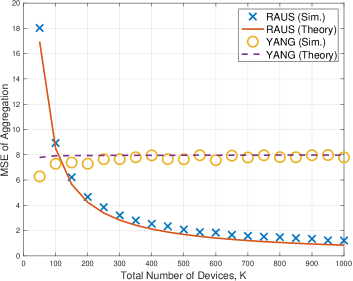
Figure 2: Performance of the RAUS and YANG approaches for different number of devices, $K$ with $L=80$ ($\bar{L}=8$ and $D=10$), $\bar{K}=10$, $N=100$, and SNR = 4 dB.

As explained in Subsection V-B, MPT can reduce the MSE in RAUS. To see this, with a fixed $L=4096$, the MSE is obtained with increasing $\bar{L}$. The results are shown in Fig. 3. Clearly, in order to decrease the MSE, we need to keep $\bar{L}$ small. This is also useful for devices with limited storage as the size of codebook or preamble pool increases with $\bar{L}$.

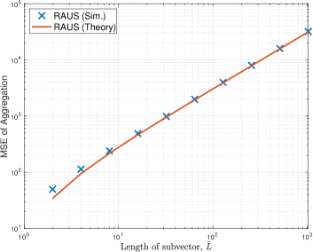
Figure 3: Performance of RAUS as a function of $\bar{L}$ when $L$ is fixed with $L=2^{12}=4096$, $K=200$, $N=100$, and SNR = 4 dB.

To see the performance of RAUS and YANG in distributed SGD, we consider the support vector classifier (SVC) with training image data sets in [24]. Only two different classes of image data sets are considered for binary linear SVC. The length of the parameter vector is $L=32\times 32\times 3=3072$ (the size of image is $32\times 32$ and each image has 3 different colors). As in [1], the cost function based on the hinge function is given by

$$C({\bf w},{\bf x}_{k})=\max(0,1-\ell_{k}({\bf w}^{\rm T}{\bf x}_{k}-w_{0}))+\lambda||{\bf w}||^{2},$$ (74)

where $\ell_{k}\in\{\pm 1\}$ is the label of data set at device $k$ (i.e. $\ell_{k}=-1$ and $+1$ for labels 0 and 1, respectively), $w_{0}$ represents the offset term, and $\lambda>0$ is the Lagrange multiplier. We assume that each device has one image and there are $K/2=500$ devices with label 0 and $K/2=500$ with label 1, i.e., there are a total of $K=1000$ devices. In addition, for simulations, we assume that $N=100$ and SNR $=10$ dB.

In Fig. 4, it is shown that the cost decreases as the number of rounds increases (up to $T=10,000$). For YANG and RAUS, the step-size is set to $\mu=0.01$ and $0.1$, respectively. Note that the step-size in YANG is smaller than that in RAUS, because the size of minibatch, $\bar{K}$, is usually smaller than the total number of devices, $K$. In particular, we consider $\bar{K}\in\{10,20,50\}$ for YANG. Clearly, as shown in Fig. 4, the steady-state cost decreases with $\bar{K}$ in YANG, which is expected from Fig. 1. For RAUS, we have two different values of $\bar{L}$, i.e., $\bar{L}\in\{8,16\}$. Since the MSE of the estimated aggregation decreases as $\bar{L}$ decreases as shown in Fig. 3, we can see that the steady-state cost becomes smaller as $\bar{L}$ decreases in RAUS.

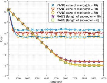
Figure 4: Convergence of distributed SGD for binary SVC when YANG and RAUS are used to upload devices’ local gradient vectors with $K=1000$, $N=100$, and SNR $=10$ dB.

VIII Concluding Remarks

For communication-efficient distributed SGD over wireless channels, we proposed an approach based on random access. In particular, in the proposed approach with a preamble-based random access scheme, we considered a one-to-one correspondence between the quantization codebook, which is used for quantizing local gradient vectors, and the preamble set, which is used for random access, so that a device can send a preamble corresponding to its quantized gradient vector. In addition, as soft weights, the access probability has been controlled to send the information of the norm of gradient vector implicitly without using additional channel resources.

We showed that the proposed approach can support a large number of devices participated in distributed SGD without increasing the time for one iteration. In fact, the performance can be improved by increasing the number of devices as the MSE of the estimated aggregation decreases with the number of devices. The MSE of the estimated aggregation was also analyzed and compared with that in [12]. From simulations, we also confirmed that the theoretical MSE obtained by asymptotic analysis is close to simulation results.

Appendix A: Bounds on $M$

In [20], it is shown that ${\cal B}_{L}(0,1)\subseteq{\rm Conv}({\cal C})$ if and only if there exists ${\bf c}\in{\cal C}$ such that $\langle{\bf x},{\bf c}\rangle\geq 1$ for any ${\bf x}\in{\cal S}^{L-1}$. Here, ${\cal S}^{n}$ represents the $n$-sphere, i.e., ${\cal S}^{n}=\{{\bf x}\in{\mathbb{R}}^{n+1}:\ ||{\bf x}||=1\}$. Thus, for uniformly distributed codewords, ${\bf c}_{m}$’s,

$$|{\cal C}|=\frac{\mbox{Area (${\cal S}^{L-1}$)}}{\mbox{Area ($\Delta$)}},$$ (75)

where $\Delta=\{{\bf x}\in{\cal S}^{L-1}:\ \langle{\bf x},{\bf c}\rangle\geq 1\}$. From (6), we have $||{\bf c}||\leq R$. Thus, $\Delta$ is the (hyper-spherical) cap with angle $\phi$ such that $\cos\phi\geq\frac{1}{||{\bf c}||}\geq\frac{1}{R}$.

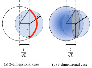
Figure 5: Upper and lower bounds on the area of cap: (a) the case of $L=2$; (b) the case of $L=3$.

In Fig. 5 (a) and (b), the areas of the cap are shown for the cases of $L=2$ (by the thick line) and $L=3$, respectively, with $\frac{1}{R}=\frac{t}{\sqrt{L}}$. The area of the cap is bounded by a half surface of a sphere of radius $r$ (upper-bound) and the volume of the slice of radius $r$. For the case of $L=2$, we have $2r<\mbox{Area of cap}<\pi r$, where $2r$ and $\pi r$ are the lower and upper bounds, respectively. Furthermore, for $L=3$, $\pi r^{2}<\mbox{Area of cap}<2\pi r^{2}$. For any $L$, it can be shown that

$$V_{L-1}(r)=\frac{\pi^{\frac{L-1}{2}}}{\Gamma\left(\frac{L+1}{2}\right)}r^{L-1} <\mbox{Area of cap}$$ (76)

$$<\frac{S_{L}(r)}{2}=\frac{\pi^{\frac{L}{2}}}{\Gamma\left(\frac{L}{2}\right)}r^{L-1}.$$ (77)

Let $\rho=\frac{1}{|{\cal C}|}$. Then, we have

$$\rho \leq\rho_{\rm ub}=\frac{S_{L}(r)}{2S_{L}(1)}=\frac{1}{2}r^{L-1}=\frac{1}{2}\left(1-\frac{t^{2}}{L}\right)^{\frac{L-1}{2}}$$ (78)

$$\rho \geq\rho_{\rm lb}=\frac{V_{L-1}(r)}{S_{L}(1)}=\frac{\Gamma\left(\frac{L}{2}\right)}{\Gamma\left(\frac{L+1}{2}\right)2\sqrt{\pi}}\left(1-\frac{t^{2}}{L}\right)^{\frac{L-1}{2}}.$$ (79)

With $t=\frac{\sqrt{L}}{R}$, it can be shown that

$$2\left(1-\frac{t^{2}}{L}\right)^{-\frac{L-1}{2}}\leq\frac{1}{\rho}\leq\sqrt{2\pi L}\left(1-\frac{t^{2}}{L}\right)^{-\frac{L-1}{2}}.$$ (80)

or, for a large $L$,

$$2e^{\frac{L}{2R^{2}}}\leq|{\cal C}|\leq\sqrt{2\pi L}e^{\frac{L}{2R^{2}}}.$$ (81)

Appendix B: MSE of $\hat{\bf g}$ in (53)

Since $\hat{\bf g}$ in (53) is unbiased, we have

$${\sf MSE}(\hat{\bf g}) ={\mathbb{E}}\left[||\hat{\bf g}-{\bf g}||^{2}\right]={\mathbb{E}}[||\hat{\bf g}||^{2}]-||{\bf g}||^{2}$$ (82)

$$=\left(\frac{V_{\rm max}}{P}\right)^{2}\left({\mathbb{E}}[||{\bf a}||^{2}]-||{\mathbb{E}}[{\bf a}]||^{2}\right).$$ (83)

Thus, to show that the variance of $\hat{\bf g}$ is finite, it is sufficient to find ${\mathbb{E}}[||{\bf a}||^{2}]$.

From (49), it can be shown that

$${\mathbb{E}}[||{\bf a}||^{2}] ={\mathbb{E}}\left[||\sum_{m}\frac{||{\bf z}_{m}||^{2}}{KN}{\bf c}_{m}||^{2}\right]$$ (84)

$$=\frac{1}{K^{2}}\biggl{(}\sum_{m}\frac{{\mathbb{E}}[||{\bf z}_{m}||^{4}]}{N^{2}}||{\bf c}_{m}||^{2}$$ (85)

$$\ \ +\sum_{m\neq m^{\prime}}\frac{{\mathbb{E}}[||{\bf z}_{m}||^{2}]{\mathbb{E}}[||{\bf z}_{m^{\prime}}||^{2}]}{N^{2}}{\bf c}_{m}^{\rm T}{\bf c}_{m^{\prime}}\biggl{)}.$$ (86)

From (46), we have

$$\frac{{\mathbb{E}}[||{\bf z}_{m}||^{4}]}{N^{2}} =3\sigma_{m}^{4}$$ (87)

$$\frac{{\mathbb{E}}[||{\bf z}_{m}||^{2}]{\mathbb{E}}[||{\bf z}_{m^{\prime}}||^{2}]}{N^{2}} =\sigma_{m}^{2}\sigma_{m^{\prime}}^{2},$$ (88)

where $\sigma_{m}^{2}=\frac{P}{V_{\rm max}}\sum_{k\in{\cal K}_{m}}||{\bf v}_{m}||+N_{0}$. Then, after some manipulations, it can be shown that

$$K^{2}{\mathbb{E}}[||{\bf a}||^{2}]=||\sum_{m}\sigma_{m}^{2}{\bf c}_{m}||^{2}+\frac{2}{N}\sum_{m}\sigma_{m}^{4}||{\bf c}_{m}||^{2}.$$ (89)

Since ${\bf c}_{m}\in{\cal C}_{\rm cp}$, we have $||{\bf c}_{m}||^{2}=L$ and

$$||\sum_{m}\sigma_{m}^{2}{\bf c}_{m}||^{2} =\sum_{l=1}^{L}(\sigma_{l}^{2}-\sigma_{L+l}^{2})^{2}L$$ (90)

$$\leq\sum_{l=1}^{L}(\sigma_{l}^{4}+\sigma_{L+l}^{4})L=L\sum_{m}\sigma_{m}^{4}.$$ (91)

Substituting (91) into (89), we have

$${\mathbb{E}}[||{\bf a}||^{2}]\leq\frac{L\left(1+\frac{2}{N}\right)}{K^{2}}\sum_{m}\sigma_{m}^{4}.$$ (92)

With $\sum_{m}\sigma_{m}^{2}=c_{1}$, it can be shown that

$$\sum_{m}\sigma_{m}^{4} \leq c_{1}^{2}=\left(\sum_{m}\frac{P}{V_{\rm max}}\sum_{k\in{\cal K}_{m}}||{\bf v}_{m}||+N_{0}\right)^{2}$$ (93)

$$=\left(\frac{P}{V_{\rm max}}\sum_{k}||{\bf v}_{k}||+MN_{0}\right)^{2}.$$ (94)

From (54), we have $||{\bf v}_{k}||=||\nabla C({\bf w},{\bf x}_{k})||\leq U$. Then, it follows that

$${\mathbb{E}}[||{\bf a}||^{2}] \leq L\left(1+\frac{2}{N}\right)\left(\frac{\frac{P}{V_{\rm max}}\sum_{k}||{\bf v}_{k}||+MN_{0}}{K}\right)^{2}$$ (95)

$$\leq L\left(1+\frac{2}{N}\right)\left(\frac{P}{V_{\rm max}}U+\frac{MN_{0}}{K}\right)^{2}.$$ (96)

Substituting (96) into (83), we have (57).

Appendix C: Derivation of (61)

From (59), we have

$$\hat{\bf g}-{\bf g}=\frac{1}{K}\sum_{k=1}^{K}\left(V_{\rm max}\beta_{k}{\bf c}_{m(k)}-||{\bf v}_{k}||\tilde{\bf v}_{k}\right).$$ (97)

Since

$${\mathbb{E}}\left[V_{\rm max}\beta_{k}{\bf c}_{m(k)}-||{\bf v}_{k}||\tilde{\bf v}_{k}\right]=0,$$

it can be shown that

$${\mathbb{E}}[||\hat{\bf g}-{\bf g}||^{2}]=\frac{1}{K^{2}}\sum_{k=1}^{K}{\mathbb{E}}\left[Z_{k}\right],$$ (98)

where $Z_{k}=||V_{\rm max}\beta_{k}{\bf c}_{m(k)}-||{\bf v}_{k}||\tilde{\bf v}_{k}||^{2}]$. Then, since

$$Z_{k} =V_{\rm max}^{2}\beta_{k}||{\bf c}_{m(k)}||^{2}+||{\bf v}_{k}||^{2}$$ (99)

$$\quad-2V_{\rm max}\beta_{k}||{\bf v}_{k}||{\bf c}_{m(k)}^{\rm T}\tilde{\bf v}_{k}$$ (100)

$$=V_{\rm max}^{2}\beta_{k}L+||{\bf v}_{k}||^{2}-2V_{\rm max}\beta_{k}||{\bf v}_{k}||{\bf c}_{m(k)}^{\rm T}\tilde{\bf v}_{k}$$ (101)

and ${\mathbb{E}}[{\bf c}_{m(k)}]=\tilde{\bf v}_{k}$, we have

$${\mathbb{E}}\left[Z_{k}\right] =V_{\rm max}^{2}{\mathbb{E}}[\beta_{k}]L+||{\bf v}_{k}||^{2}-2V_{\rm max}{\mathbb{E}}[\beta_{k}]||{\bf v}_{k}||$$ (102)

$$=LV_{\rm max}||{\bf v}_{k}||-||{\bf v}_{k}||^{2}.$$ (103)

Substituting (103) into (98), we have (61).

References

- [1] C. M. Bishop, Pattern Recognition and Machine Learning (Information Science and Statistics). Berlin, Heidelberg: Springer-Verlag, 2006.
- [2] I. Goodfellow, Y. Bengio, and A. Courville, Deep Learning. MIT Press, 2016. http://www.deeplearningbook.org.
- [3] J. Verbraeken, M. Wolting, J. Katzy, J. Kloppenburg, T. Verbelen, and J. S. Rellermeyer, “A survey on distributed machine learning,” ACM Comput. Surv., vol. 53, Mar. 2020.
- [4] J. Konecný, H. B. McMahan, D. Ramage, and P. Richtárik, “Federated optimization: Distributed machine learning for on-device intelligence,” ArXiv, vol. abs/1610.02527, 2016.
- [5] Q. Yang, Y. Liu, T. Chen, and Y. Tong, “Federated machine learning: Concept and applications,” ACM Trans. Intell. Syst. Technol., vol. 10, pp. 12:1–12:19, Jan. 2019.
- [6] L. Bottou, F. E. Curtis, and J. Nocedal, “Optimization methods for large-scale machine learning,” SIAM Review, vol. 60, no. 2, pp. 223–311, 2018.
- [7] S. R. Pokhrel and J. Choi, “Improving TCP performance over WiFi for Internet of Vehicles: A federated learning approach,” IEEE Trans. Vehicular Technology, vol. 69, no. 6, pp. 6798–6802, 2020.
- [8] S. Samarakoon, M. Bennis, W. Saad, and M. Debbah, “Distributed federated learning for ultra-reliable low-latency vehicular communications,” IEEE Trans. Communications, vol. 68, no. 2, pp. 1146–1159, 2020.
- [9] S. Savazzi, M. Nicoli, and V. Rampa, “Federated learning with cooperating devices: A consensus approach for massive IoT networks,” IEEE Internet of Things Journal, vol. 7, no. 5, pp. 4641–4654, 2020.
- [10] M. M. Amiri and D. Gündüz, “Federated learning over wireless fading channels,” IEEE Trans. Wireless Communications, vol. 19, no. 5, pp. 3546–3557, 2020.
- [11] G. Zhu, Y. Wang, and K. Huang, “Broadband analog aggregation for low-latency federated edge learning,” IEEE Trans. Wireless Communications, vol. 19, no. 1, pp. 491–506, 2020.
- [12] K. Yang, T. Jiang, Y. Shi, and Z. Ding, “Federated learning via over-the-air computation,” IEEE Trans. Wireless Communications, vol. 19, no. 3, pp. 2022–2035, 2020.
- [13] B. Nazer and M. Gastpar, “Computation over multiple-access channels,” IEEE Trans. Information Theory, vol. 53, no. 10, pp. 3498–3516, 2007.
- [14] M. Goldenbaum, H. Boche, and S. Stańczak, “Harnessing interference for analog function computation in wireless sensor networks,” IEEE Trans. Signal Processing, vol. 61, pp. 4893–4906, Oct 2013.
- [15] C. Bockelmann, N. Pratas, H. Nikopour, K. Au, T. Svensson, C. Stefanovic, P. Popovski, and A. Dekorsy, “Massive machine-type communications in 5G: physical and MAC-layer solutions,” IEEE Communications Magazine, vol. 54, pp. 59–65, Sep 2016.
- [16] J. Ding, M. Nemati, C. Ranaweera, and J. Choi, “IoT connectivity technologies and applications: A survey,” IEEE Access, vol. 8, pp. 67646–67673, 2020.
- [17] J. Choi and S. R. Pokhrel, “Federated learning with multichannel ALOHA,” IEEE Wireless Communications Letters, vol. 9, no. 4, pp. 499–502, 2020.
- [18] J. Kim, G. Lee, S. Kim, T. Taleb, S. Choi, and S. Bahk, “Two-step random access for 5G system: Latest trends and challenges,” IEEE Network, pp. 1–7, 2020.
- [19] J. Choi, “On fast retrial for two-step random access in MTC,” IEEE Internet of Things J., vol. 8, no. 3, pp. 1428–1436, 2021.
- [20] V. Gandikota, R. K. Maity, and A. Mazumdar, “vqSGD: Vector quantized stochastic gradient descent,” CoRR, vol. abs/1911.07971, 2019.
- [21] J. Bernstein, Y.-X. Wang, K. Azizzadenesheli, and A. Anandkumar, “signSGD: Compressed optimisation for non-convex problems,” in Proceedings of the 35th International Conference on Machine Learning (J. Dy and A. Krause, eds.), vol. 80 of Proceedings of Machine Learning Research, (Stockholmsmässan, Stockholm Sweden), pp. 560–569, PMLR, 10–15 Jul 2018.
- [22] D. Alistarh, D. Grubic, J. Li, R. Tomioka, and M. Vojnovic, “QSGD: Communication-efficient SGD via gradient quantization and encoding,” in Advances in Neural Information Processing Systems (I. Guyon, U. V. Luxburg, S. Bengio, H. Wallach, R. Fergus, S. Vishwanathan, and R. Garnett, eds.), vol. 30, pp. 1709–1720, Curran Associates, Inc., 2017.
- [23] T. L. Marzetta, “Noncooperative cellular wireless with unlimited numbers of base station antennas,” IEEE Trans. Wireless Communications, vol. 9, pp. 3590–3600, Nov. 2010.
- [24] A. Krizhevsky and G. Hinton, “Learning multiple layers of features from tiny images,” Master’s thesis, Department of Computer Science, University of Toronto, 2009.