Alignments of Triad Phases
in 1D Burgers and 3D Navier-Stokes Flows

Abstract

The goal of this study is to analyze the fine structure of nonlinear modal interactions in different 1D Burgers and 3D Navier-Stokes flows. This analysis is focused on preferential alignments characterizing the phases of Fourier modes participating in triadic interactions, which are key to determining the nature of energy fluxes between different scales. We develop novel diagnostic tools designed to probe the level of coherence among triadic interactions realizing different flow scenarios. We consider extreme (in the sense of maximizing the growth of enstrophy in finite time) 1D viscous Burgers flows and 3D Navier-Stokes flows which are complemented by singularity-forming inviscid Burgers flows as well as viscous Burgers flows and Navier-Stokes flows corresponding to generic turbulent and simple unimodal initial data, such as the Taylor-Green vortex. The main finding is that while the extreme viscous Burgers and Navier-Stokes flows reveal the same relative level of enstrophy amplification by nonlinear effects, this behaviour is realized via modal interactions with vastly different levels of coherence. In the viscous Burgers flows the flux-carrying triads have phase values which saturate the nonlinearity thereby maximizing the energy flux towards small scales. On the other hand, in 3D Navier-Stokes flows with the extreme initial data the energy flux to small scales is realized by a very small subset of helical triads, with the flux-carrying triads showing again a high level of coherence, but with their phases taking a broader range of preferred values which form complex time-dependent patterns. The second main finding concerns the role of initial coherence. Comparison of the flows resulting from the extreme and generic initial conditions shows striking similarities between these two types of flows, for the 1D viscous Burgers equation as well as the 3D Navier-Stokes equation. The third main finding concerns 3D Navier-Stokes flows resulting from the Taylor-Green initial condition. On the one hand, as expected, the fluxes in this case are several times smaller than in the extreme or generic cases. On the other hand, the flux-carrying triads in this case display much more rigid patterns of phase coherence, with persistent narrow bands of preferred phase values. Finally, we find that the paradigm based on the instability assumption due to Waleffe (1992) holds true at all scales for the 3D Navier-Stokes flows, with some variations. The flows resulting from the extreme or generic initial conditions show a quantitative agreement with simulations of statistically stationary turbulence by Alexakis & Biferale (2018) concerning the inverse-cascade behaviour at the inertial range of homochiral triads (i.e., triads with the same helical content, or Class I in Waleffe’s notation). In contrast, in the flow resulting from the Taylor-Green initial condition, the inverse-cascade behaviour is dominated by heterochiral triads of Class II in Waleffe’s notation.

1 Introduction

Understanding and quantifying the most extreme forms of behaviour allowed for by the Navier-Stokes system describing the motion of viscous incompressible fluids remains a key outstanding problem in theoretical fluid dynamics. By “extreme behaviour” we mean situations where certain flow quantities attain very large or very small values approaching or saturating mathematically rigorous bounds on these quantities. Providing answers to such questions is important for our understanding of fundamental performance limitations inherent in elementary physical processes underlying fluid motion such as transport, mixing, etc. A special case of this class of problems, which is particularly important from the theoretical point of view, concerns the question whether or not solutions to the three-dimensional (3D) Navier-Stokes system and some other related models may form singularities in finite time (Doering, 2009). Singularity formation implies that the solution develops features preventing it from satisfying the equation in the classical sense, i.e., pointwise in space and in time. Such features are usually hypothesized to have the form of non-differentiable accumulations of vorticity. Needless to say, should such singularities indeed form, this would invalidate the equation as a physically consistent model for fluid flow. In recognition of its significance, the Navier-Stokes regularity problem has been named by the Clay Mathematics Institute one of its seven “Millennium Problems” (Fefferman, 2000). However, progress on this problem has been rather slow (Robinson, 2020).

As highlighted by Robinson (2020) in one of his concluding remarks, progress concerning possibly singular behaviour in the Navier-Stokes and related flow models will require a better understanding of the fine structure of interactions between modes. The goal of the present study is thus to provide new insights about this problem by analyzing both generic and extreme flow evolutions using diagnostic tools specifically designed to shed light on the nature of triadic interactions. As described in more detail below, the extreme flows we consider extremize the enstrophy as a physically relevant quantity which also plays the role of an indicator of the regularity of solutions.

All models we consider are defined on spatially periodic domains $\Omega:=[0,1]^{d}$, where $d=1,3$ is the dimension and “$:=$” means “equal to by definition”, such that they are subject to periodic boundary conditions. Flows of viscous incompressible fluids in 3D are governed by the Navier-Stokes system

$$\left({\partial\over\partial t}-\nu\boldsymbol{\nabla}^{2}\right)\mathbf{{u}}(\mathbf{x},t) =-\boldsymbol{\nabla}p(\mathbf{x},t)-\mathbf{{u}}(\mathbf{x},t)\cdot\boldsymbol{\nabla}\mathbf{{u}}(\mathbf{x},t)\qquad\qquad {\mathbf{x}}\in\Omega,\ t>0$$ (1a)

$$\boldsymbol{\nabla}\cdot\mathbf{{u}}(\mathbf{x},t) =0 {\mathbf{x}}\in\Omega,\ t>0$$ (1b)

$${\mathbf{u}}({\mathbf{x}},0) ={\mathbf{u}}_{0}({\mathbf{x}}) {\mathbf{x}}\in\Omega,\ t=0,$$ (1c)

where ${\mathbf{u}}({\mathbf{x}},t)$ and $p({\mathbf{x}},t)$ are the velocity vector field and the scalar pressure field whereas $\nu$ is the kinematic viscosity. Equations (1a) and (1b) represent, respectively, the conservation of momentum and mass, whereas ${\mathbf{u}}_{0}$ is the initial condition. Key quantities characterizing solutions of the Navier-Stokes system (1) include the kinetic energy ${\mathcal{K}}({\mathbf{u}})$, enstrophy ${\mathcal{E}}({\mathbf{u}})$ and helicity ${\mathcal{H}}({\mathbf{u}})$ defined as

$${\mathcal{K}}({\mathbf{u}}) :=\frac{1}{2}\int_{\Omega}|{\mathbf{u}}|^{2}\,\mathrm{d}{\mathbf{x}},$$ (2a)

$${\mathcal{E}}({\mathbf{u}}) :=\frac{1}{2}\int_{\Omega}|\boldsymbol{\omega}|^{2}\,\mathrm{d}{\mathbf{x}}{=\frac{1}{2}\int_{\Omega}|\boldsymbol{\nabla}{\mathbf{u}}|^{2}\mathrm{d}{\mathbf{x}},}$$ (2b)

$${\mathcal{H}}({\mathbf{u}}) :=\int_{\Omega}{\mathbf{u}}\cdot\boldsymbol{\omega}\,\mathrm{d}{\mathbf{x}},$$ (2c)

where $\boldsymbol{\omega}:=\boldsymbol{\nabla}\times\mathbf{{u}}$ is the vorticity. With a slight abuse of notations, we will sometimes write ${\mathcal{E}}(t)={\mathcal{E}}({\mathbf{u}}(t))$. We will also use the Sobolev space $H^{1}(\Omega)$ of functions with square-integrable gradients with the norm defined as $\|{\mathbf{u}}\|_{H^{1}}^{2}:=\int_{\Omega}|{\mathbf{u}}|^{2}+|\boldsymbol{\nabla}{\mathbf{u}}|^{2}\,\mathrm{d}{\mathbf{x}}$ (Adams & Fournier, 2005).

As a commonly-used simplified model for the Navier-Stokes system (1), we will also consider the one-dimensional (1D) viscous Burgers system

$${\partial u(x,t)\over\partial t}+u(x,t){\partial u(x,t)\over\partial x}-\nu{\partial^{2}u(x,t)\over\partial x^{2}} =0\qquad\qquad x\in\Omega,\ t>0,$$ (3a)

$$u(x,0) =u_{0}(x) x\in\Omega,\ t=0$$ (3b)

and its inviscid version

$${\partial u(x,t)\over\partial t}+u(x,t){\partial u(x,t)\over\partial x} =0\qquad\qquad x\in\Omega,\ t>0,$$ (4a)

$$u(x,0) =u_{0}(x) x\in\Omega,\ t=0,$$ (4b)

where $u_{0}$ is the initial condition. In the Burgers flows the kinetic energy and the enstrophy are defined analogously to (2a) and (2b).

The question of the existence of solutions to the 1D Burgers problems is well understood (Kreiss & Lorenz, 2004). While the viscous problem (3) is globally well-posed, the inviscid Burgers problem (4) is known to produce a finite-time blow-up for all nonconstant initial data $u_{0}\in H^{1}(\Omega)$ (more specifically, the solutions blow up by developing an infinitely steep front). On the other hand, as already indicated above, the question of existence of classical (smooth) solutions to the 3D Navier-Stokes system (1) remains open (Doering, 2009; Robinson, 2020). One of the most useful conditional regularity results asserts that the solution ${\mathbf{u}}(t)$ of (1) remains smooth on the time interval $[0,T]$ provided ${\mathcal{E}}(t)<\infty$, $\forall t\in[0,T]$ (Foias & Temam, 1989), making the enstrophy a convenient indicator of the regularity of solutions. The evolution of the kinetic energy and the enstrophy is governed by the system (Doering, 2009)

$$\frac{d{\mathcal{K}}({\mathbf{u}}(t))}{dt} =-2\nu{\mathcal{E}}({\mathbf{u}}(t)),$$ (5a)

$$\frac{d{\mathcal{E}}({\mathbf{u}}(t))}{dt} ={\mathcal{R}}({\mathbf{u}}(t))\leq-\nu\frac{{\mathcal{E}}({\mathbf{u}}(t))^{2}}{{\mathcal{K}}({\mathbf{u}}(t))}+\frac{c}{\nu^{3}}{\mathcal{E}}({\mathbf{u}}(t))^{3},$$ (5b)

where ${\mathcal{R}}({\mathbf{u}}(t)):=-\nu\int_{\Omega}|\Delta{\mathbf{u}}|^{2}\,\mathrm{d}{\mathbf{x}}+\int_{\Omega}{\mathbf{u}}\cdot\nabla{\mathbf{u}}\cdot\Delta{\mathbf{u}}\,d{\mathbf{x}}$ and $c$ is a known constant. Using (5b), one can then derive the estimate

$${\mathcal{E}}({\mathbf{u}}(t))\leq\frac{{\mathcal{E}}_{0}}{\sqrt{1-\frac{27}{4\,\pi^{4}\,\nu^{3}}\,{\mathcal{E}}_{0}^{2}\,t}},$$ (6)

where ${\mathcal{E}}_{0}:={\mathcal{E}}({\mathbf{u}}_{0})$, which is one of the best results of this type available to-date. However, since the upper bound on the right-hand side (RHS) of this estimate becomes unbounded when $t\rightarrow 4\,\pi^{4}\,\nu^{3}/(27\,{\mathcal{E}}_{0}^{2})$, finite-time blow-up cannot be ruled out based on this estimate.

In order to probe the question whether the enstrophy might become unbounded in finite time in 3D Navier-Stokes flows, the following family of PDE-constrained optimization problems was solved by Kang et al. (2020)

$$\widetilde{\mathbf{u}}_{0;{\mathcal{E}}_{0},T}=\operatorname{argmax}_{{\mathbf{u}}_{0}\in H^{1}(\Omega),\ \boldsymbol{\nabla}\cdot{\mathbf{u}}_{0}=0}{\mathcal{E}}({\mathbf{u}}(T))\quad\textrm{subject to}\ \left\{\begin{aligned} &\mbox{{{S}ystem}}\ \eqref{eq:3DNS_u}\\ &{\mathcal{E}}({\mathbf{u}}_{0})={\mathcal{E}}_{0}\end{aligned}\right.,$$ (7)

where, for specified values of $T>0$ and ${\mathcal{E}}_{0}>0$, the extreme initial conditions $\widetilde{\mathbf{u}}_{0;{\mathcal{E}}_{0},T}$ with fixed enstrophy ${\mathcal{E}}_{0}$ were found, such that the corresponding enstrophy ${\mathcal{E}}({\mathbf{u}}(T))$ at the final time $T$ is maximal. Optimization problems of this type are efficiently solved numerically using adjoint-based gradient methods (Protas et al., 2004). While no evidence was found for unbounded growth of enstrophy in such extreme Navier-Stokes flows, solving problem (7) for a broad range of ${\mathcal{E}}_{0}$ and $T$ revealed the following empirical relation characterizing how the largest attained enstrophy scales with the initial enstrophy ${\mathcal{E}}_{0}$ in the most extreme scenarios (Kang et al., 2020)

$$\max_{T>0}{\mathcal{E}}(T)\ \sim\ {\mathcal{E}}_{0}^{3/2}.$$ (8)

While blow-up is ruled out in viscous Burgers flows, the question whether the corresponding a priori estimates on the growth of enstrophy are sharp or have room for improvement is quite pertinent as they are obtained in a similar way to (6). In order to address this question, a family of optimization problems of the type (7) was solved for the 1D viscous Burgers system (3) by Ayala & Protas (2011). Interestingly, the extreme behaviour found in this way also obeys relation (8). Our present study is motivated by the observation that extreme behaviour in 1D Burgers systems and 3D Navier-Stokes systems must be characterized by nonlinear energy transfers towards modes corresponding to small spatial scales. We aim to understand and compare the fine structure of the nonlinear interactions between modes which give rise to the extreme behaviour described by relation (8) in 1D Burgers and 3D Navier-Stokes flows. We will also compare these flows to the flow evolutions corresponding to generic and some simple initial data, as well as to inviscid Burgers flows which do form singularities in finite time.

Since the seminal work by Kraichnan (1959), it has been established that nonlinear triad interactions play a pivotal role in the mechanisms of energy transfer across spatial scales in 2D or 3D Navier-Stokes flows, leading to cascades of energy, enstrophy and helicity with direct or inverse directions, depending on the dimension. Specifically for 3D Navier-Stokes flows, the work by Waleffe (1992) based on analysis of helical triads established a paradigm termed “the instability assumption” whereby unstable modes in helical triads determine the statistically expected directions of spectral energy fluxes across scales. A recent result by Moffatt (2014) shows that a Galerkin-truncated system consisting of a single triad does not produce a reasonable time evolution when compared with the evolution of the real system. It thus indicates that triad interactions must always be considered in the context of a network of multiple triad interactions, where energy exchanges in all directions are in principle allowed, as otherwise a non-physical recurrent behaviour would be obtained. Waleffe’s paradigm has been confirmed in several works (Rathmann & Ditlevsen, 2017; Alexakis, 2017; Alexakis & Biferale, 2018) and has motivated new research concerning the effect of triad interactions on the directions of the cascades of energy and other invariants. These questions were recently investigated by Biferale et al. (2012, 2013); Sahoo & Biferale (2015) who used alternative models to numerically “probe” the effect of triad interactions by arbitrarily eliminating some modes or some triad interactions from the equations, depending on various criteria such as the relative helicities of the modes involved.

A vast majority of the works cited above have focused on theoretical studies and/or on analyzing the energy and helicity spectra of numerically computed flows, along with their corresponding spectral fluxes. As the spectral fluxes are the main quantities of interest when looking at energy cascades across scales, it is interesting to note the following research gap: an analysis of these spectral fluxes in terms of the dynamically evolving spectral phases (i.e., the arguments of the complex spectral coefficients) has been absent from practically all previous works, except perhaps in shell models where a relevant quantity that somehow bridges phases and fluxes is the three-point correlator which provides a good diagnostic of flux cascades (De Pietro et al., 2015; Rathmann & Ditlevsen, 2016). This lack of studies of phase dynamics (or statistics thereof) in the literature persists despite the fact that researchers are well aware of the fact that any physical field whose spectral phases are random and uniformly distributed over time displays Gaussian statistics along with strictly zero energy transfer (Alexakis & Biferale, 2018), which is equivalent to the statement that the presence of energy cascades and intermittency implies nontrivial phase correlations. This research gap not only applies to the study of the 2D or 3D Navier-Stokes equations, but also to many other systems, including the 1D Burgers equations. In our present study we intend to close this gap by introducing and studying relevant quantities related to the spectral phases. One of us was a collaborator on a number of preliminary studies of the 1D Burgers equation and models thereof (Buzzicotti et al., 2016; Murray & Bustamante, 2018), where the spectral fluxes of energy were obtained explicitly in terms of the magnitudes of the Fourier coefficients along with the less known Fourier triad phases which are linear combinations of the three phases of the complex Fourier modes involved in a triad interaction. In these works it was evident that the main mechanism responsible for the strong energy fluxes across scales, observed in the 1D Burgers system, is the so-called alignment of triad phases, namely, the tendency of triad phases to cluster around values that maximize the spectral fluxes towards small scales. This alignment is dynamical and is controlled in part by the presence of stable fixed points in the evolution equations for the phases. Moreover, in the 1D Burgers system this alignment seems to entail sustained synchronizations of the triad phases, namely, a collective behaviour whereby a large proportion of triad phases align over a wide range of spatial scales and over long time intervals. Going beyond that, Murray (2017) applied this idea to the study of 3D Navier-Stokes flows with stochastic forcing at large spatial scales. These analyses showed that, statistically, there is a slight preference for helical triad phases to align so as to maximize the fluxes towards small scales. Specifically, when restricting attention to $5\%$ of the most energetic modes at each reciprocal length scale, the probability density functions of helical triad phases show wide alignment peaks with values of only 7% above the uniform value. Remarkably, such a slight preference for alignment of triad phases is enough to produce significant energy flux cascades. A possible explanation for this is that the coherent structures associated with aligned triad phases have a low dimensionality, perhaps even close to one.

Our present study aims to understand, from the point of view of triad phases, the fine structure of mode interactions arising in extreme transient solutions where strong energy transfers are observed. Our most important result is that while the extreme 1D Burgers and 3D Navier-Stokes flows obey the same scaling relation (8) for the maximum growth of enstrophy, this behaviour is achieved through vastly different levels of synchronization in the two cases. In 1D Burgers flows all triads involving energy-containing Fourier modes align so as to maximize the energy flux towards small scales. On the other hand, in 3D Navier-Stokes flows energy transfer to small scales is realized by only a small subset of the triads corresponding to preferred phase angles forming complex spatio-temporal patterns. The second main finding is that removing the spatial coherence from the extreme initial data in both 1D Burgers and 3D Navier-Stokes flows (by randomizing the Fourier phases while retaining the magnitudes of the Fourier coefficients) does not profoundly change the nature of triadic interactions and the resulting fluxes in these flows.

The structure of the paper is as follows: the specific flow problems we will analyze, specified in terms of their initial data, are defined in the next section; then, in § 3, we introduce the diagnostics we will employ to characterize the structure of the modal interactions; our results are presented in § 4, whereas discussion and final conclusions are deferred to § 5; some technical material is collected in three appendices.

2 Flow problems

In this section we introduce the flow problems we will investigate. Each of these problems is defined by a combination a governing system (1D viscous or inviscid Burgers (3)–(4), or the 3D Navier-Stokes system (1)) and one of the initial conditions given below. Information about which initial conditions are used with the different models is summarized in table 1. Some combinations of governing systems and initial data are not considered as they do not provide additional interesting insights. In agreement with the studies in which the different initial conditions were originally obtained, the viscosity coefficient will be equal to $\nu=0.001$ in the 1D viscous Burgers system (3) and to $\nu=0.01$ in the 3D Navier-Stokes system (1).

2.1 Unimodal initial conditions

The simplest initial conditions have the form of the product of single Fourier harmonics with low wavenumbers in each spatial variable. For the 1D Burgers equation, both inviscid and viscous, it will therefore take the form

$$u_{0}(x)=A\sin(2\pi x),\quad x\in\Omega,$$ (9)

where $A>0$ is a constant adjusted such that the initial condition has prescribed enstrophy ${\mathcal{E}}_{0}$. We note that for the inviscid Burgers equation (4) the constant $A$ plays no role, since the solution corresponding to $A=1$ is obtained by rescaling the time $t$ as $A^{-1}t$.

For the 3D Navier-Stokes system (1) the corresponding unimodal initial condition will have the form of the Taylor-Green vortex (Taylor & Green, 1937) with the velocity components given by

$$u_{1}(x_{1},x_{2},x_{3}) =A\sin(2\pi x_{1})\cos(2\pi x_{2})\cos(2\pi x_{3}),$$ (10a)

$$u_{2}(x_{1},x_{2},x_{3}) =-A\cos(2\pi x_{1})\sin(2\pi x_{2})\cos(2\pi x_{3}),\qquad[x_{1},x_{2},x_{3}]^{T}\in\Omega,$$ (10b)

$$u_{3}(x_{1},x_{2},x_{3}) =0,$$ (10c)

where $A>0$ is again an adjustable constant. We remark that this initial condition has a long history in studies of extreme behaviour in incompressible flows (Brachet et al., 1983; Brachet, 1991; Bustamante & Brachet, 2012; Ayala & Protas, 2017).

2.2 Extreme initial conditions

For the Navier-Stokes systems (1), the “extreme” initial condition is defined as the initial data which for a given initial enstrophy ${\mathcal{E}}_{0}$ produces the largest possible growth of enstrophy in finite time. It is thus given by $\widetilde{\mathbf{u}}_{{\mathcal{E}}_{0}}=\max_{T>0}\widetilde{\mathbf{u}}_{0;{\mathcal{E}}_{0},T}$, where $\widetilde{\mathbf{u}}_{0;{\mathcal{E}}_{0},T}$ is a solution of the optimization problem (7) with fixed $T$ and ${\mathcal{E}}_{0}$. For each value of ${\mathcal{E}}_{0}$, $\widetilde{T}_{{\mathcal{E}}_{0}}:=\operatorname{argmax}_{T>0}\widetilde{u}_{0;{\mathcal{E}}_{0},T}$ is then the time when the largest growth of enstrophy is achieved. An example of such an extreme initial condition $\widetilde{\mathbf{u}}_{{\mathcal{E}}_{0}}$ obtained at ${\mathcal{E}}_{0}=500$ is shown in figure 2 (Kang et al., 2020). We see that this field has the form of three perpendicular pairs of antiparallel vortex tubes and, as discussed in detail by Kang et al. (2020), the resulting flow evolution (which maximizes the enstrophy at the final time $\widetilde{T}_{{\mathcal{E}}_{0}}$) is marked by a series of reconnection events. Our analysis of the 3D Navier-Stokes flows in § 4.2 will focus on the case with ${\mathcal{E}}_{0}=250$. The extreme initial conditions for the 1D viscous Burgers system (3) are obtained analogously as $\widetilde{u}_{0;{\mathcal{E}}_{0}}=\max_{T>0}\widetilde{u}_{0;{\mathcal{E}}_{0},T}$, where $\widetilde{u}_{0;{\mathcal{E}}_{0},T}$ are the solutions of a suitably adapted optimization problem (7) with fixed ${\mathcal{E}}_{0}$ and $T$, cf. figure 2 (Ayala & Protas, 2011). Our analysis of the 1D Burgers flows in § 4.1 will focus on the case with ${\mathcal{E}}_{0}=100$.

    

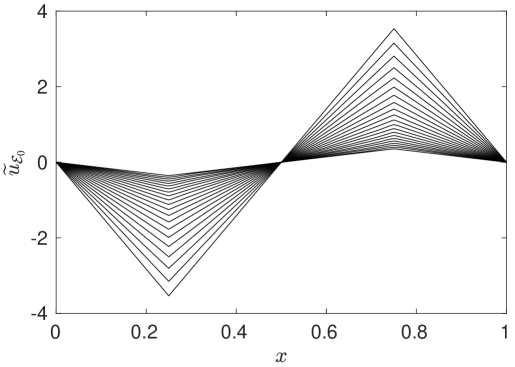
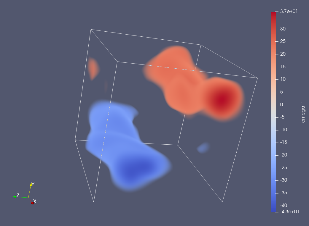
(a) $\widetilde{\omega}_{1}$

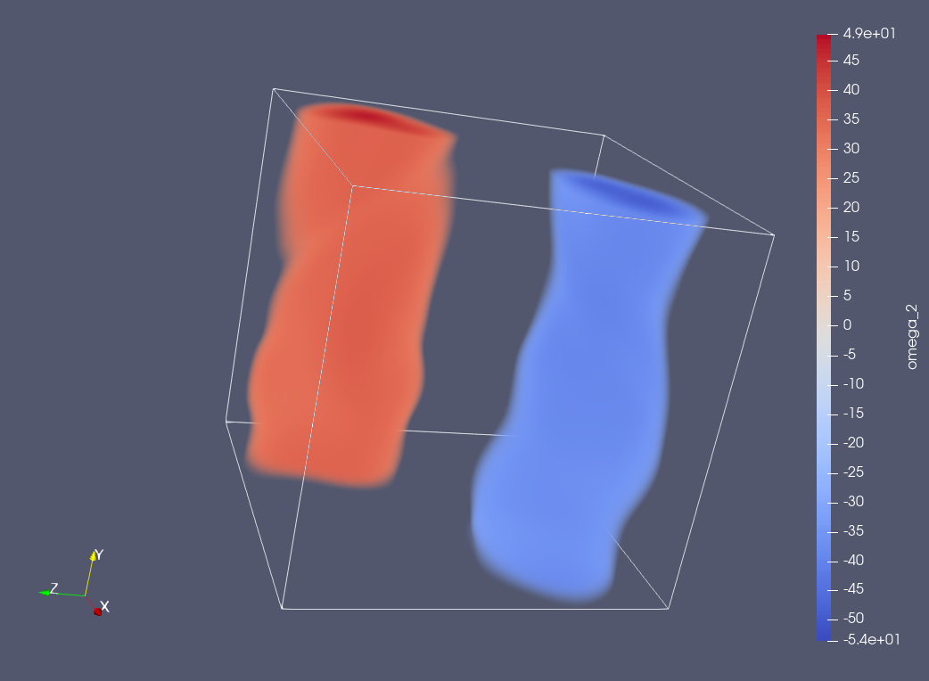
(b) $\widetilde{\omega}_{2}$

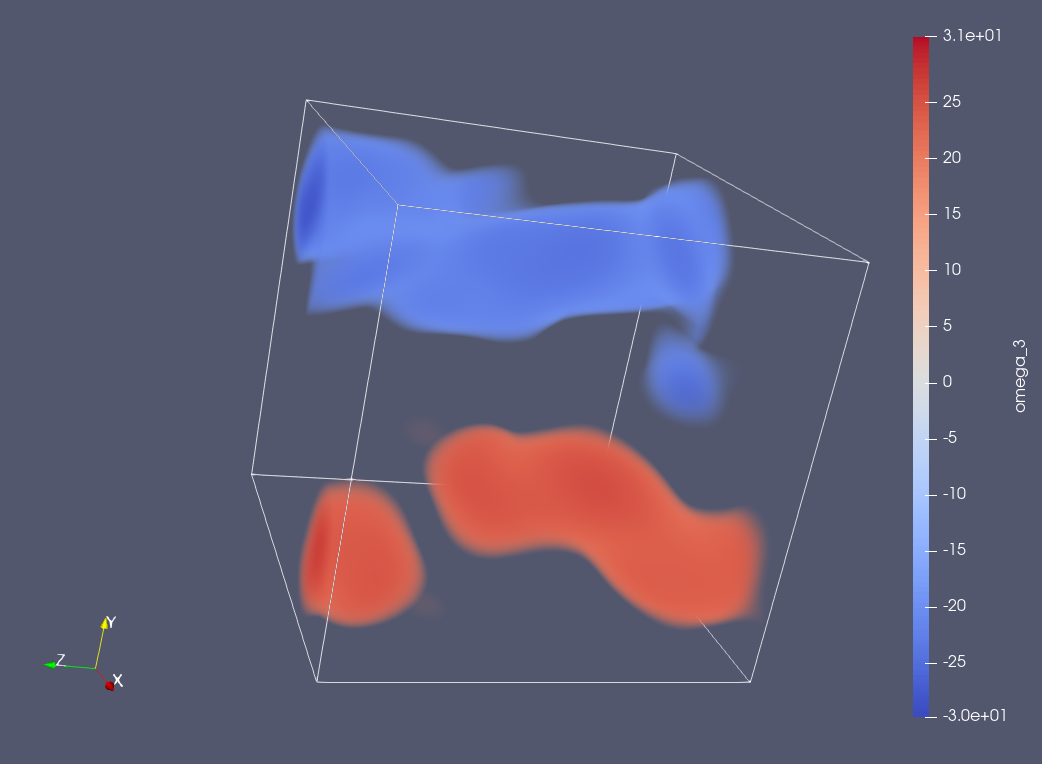
(c) $\widetilde{\omega}_{3}$

Figure 1: Vorticity components of the optimal initial condition $\widetilde{\mathbf{u}}_{0;{\mathcal{E}}_{0},\widetilde{T}_{{\mathcal{E}}_{0}}}$ obtained by solving the finite-time optimization problem (7) for the initial enstrophy ${\mathcal{E}}_{0}=500$ and the corresponding optimal length $\widetilde{T}_{{\mathcal{E}}_{0}}=0.17$ of the time interval (Kang et al., 2020).

Figure 2: Extreme initial conditions $\widetilde{u}_{0;{\mathcal{E}}_{0}}$ for the 1D Burgers equation (3) obtained by solving a family of finite-time optimization problems analogous to (7) for different values of the initial enstrophy ${\mathcal{E}}_{0}\in[1,100]$ and the corresponding optimal time windows $\widetilde{T}_{{\mathcal{E}}_{0}}$ (larger values of ${\mathcal{E}}_{0}$ correspond to increased magnitude of $\widetilde{u}_{0;{\mathcal{E}}_{0}}$, Ayala & Protas (2011)).

Since for all nonconstant initial conditions $u_{0}$ the inviscid Burgers system (4) develops a singularity in finite time, in the sense that ${\mathcal{E}}(t)\rightarrow\infty$ as $t\nearrow t^{*}$, where $t^{*}$ is the blow-up time (Kreiss & Lorenz, 2004), an optimization problem of the type (7) is not well-defined for this system. As a counterpart to the optimization problem (7) for the inviscid Burgers system (4), one might therefore think of the problem of finding initial condition $u_{0}\in H^{1}(\Omega)$ with prescribed enstrophy ${\mathcal{E}}_{0}>0$ such that the corresponding solution blows up in the shortest time $\tilde{t}^{*}$. However, as shown in Appendix A, such a problem is not in fact well posed since $\inf_{u_{0}}t^{*}(u_{0})=0$ with ${\mathcal{E}}(u_{0})={\mathcal{E}}_{0}<\infty$. However, formally extrapolating the extreme initial data $\widetilde{u}_{0;{\mathcal{E}}_{0}}$ shown in figure 2 to the limit ${\mathcal{E}}_{0}\rightarrow\infty$ leads to the following extreme initial data for the inviscid Burgers system

$$\widetilde{u}_{0}(x)=A\left(4\left|x-\frac{1}{2}\right|-1\right),\quad x\in\Omega.$$ (11)

We note that $\widetilde{u}_{0}$ in (11) is piecewise-linear, hence it is a $H^{1}$ function.

2.3 Generic initial conditions

For the viscous Burgers system (3), the “generic” initial condition is obtained from the extreme initial condition $\widetilde{u}_{0;{\mathcal{E}}_{0}}$ by decomposing this field in a Fourier series (12) and randomizing the phases of the Fourier coefficients. This is done by replacing the original phase in each of the Fourier coefficients with a random number uniformly distributed over $[0,2\pi]$ while retaining the magnitude of the coefficient. For the Navier-Stokes system (1) the generic initial condition is obtained from the extreme initial data $\widetilde{\mathbf{u}}_{{\mathcal{E}}_{0}}$ in a similar manner, except that randomization is performed on the phases of the coefficients $u_{{\mathbf{k}}}^{\pm}$ of the helical-wave decomposition (19), rather than using the Fourier decomposition (18), which ensures that the resulting field remains divergence-free (see § 3.2.1 for additional details).

We note that, as a result of the parity symmetry (39) characterizing the three initial conditions for the 3D Navier-Stokes system, the helicity remains identically zero, ${\mathcal{H}}(t)=0,\;\forall t\geq 0$, in the resulting flows. As shown in Appendix B, this observation will significantly simplify our analysis of the results in § 4.2.

	1D inviscid Burgers (4)	1D viscous Burgers (3)	3D Navier-Stokes (1)
unimodal (9)	$\checkmark$		$\checkmark$
extreme (7)	$\checkmark$	$\checkmark$	$\checkmark$
generic		$\checkmark$	$\checkmark$

Table 1: Summary information specifying which initial conditions are used with different governing systems.

3 Diagnostics

In this section we introduce a number of diagnostic quantities which will allow us to characterize the dynamics of energy transfers in terms of the evolution of triad phases in our model problems. These derivations are based on Murray & Bustamante (2018) for 1D Burgers flows (§ 3.1) and on Murray (2017) for 3D Navier-Stokes flows (§ 3.2).

3.1 Fourier Triad Phases and Fluxes in 1D Burgers Flows

The solution $u(x,t)$ of the 1D Burgers equation, either inviscid (4) or viscous (3), on a periodic domain can be conveniently represented in terms of its Fourier series

$$u(x,t)=\sum_{k\in\mathbb{Z}}e^{2\pi ikx}\widehat{u}_{k}(t),$$ (12)

where $k$ are the wavenumbers restricted to the set of integers $\mathbb{Z}$ due to the assumed periodicity. The dynamic content of the $k$th mode is expressed by its complex-valued Fourier coefficient $\widehat{u}_{k}(t)$ which, given that the solution $u(x,t)$ is real-valued, is subject to the condition of conjugate symmetry $\widehat{u}_{-k}(t)=\widehat{u}_{k}^{*}(t)$, $\forall k\in\mathbb{Z}$, where ^∗ denotes complex conjugation. Using this representation, the governing partial differential equation (PDE) can be decomposed into a set of ordinary differential equations (ODEs) which describe the time evolution of each individual Fourier mode. We focus our discussion here on the viscous problem (3) with the results for the inviscid problem (4) obtained simply by setting $\nu=0$. For each Fourier mode we use the polar representation $\widehat{u}_{k}(t)=a_{k}(t)e^{i\phi_{k}(t)}$, where $a_{k}(t)=|\widehat{u}_{k}(t)|$ is the mode amplitude and $\phi_{k}(t)=\arg[\widehat{u}_{k}(t)]$ the mode phase. In terms of the Fourier-space representation, equation (3a) then takes the form $\frac{\partial\widehat{u}_{k}}{\partial t}=-{\pi ik}\sum_{k_{1}}\,\widehat{u}_{k_{1}}\widehat{u}_{k-k_{1}}-4\nu\pi^{2}k^{2}\widehat{u}_{k}$. The core of the dynamics is the quadratic convolution term, a term that globally conserves energy by redistributing it amongst Fourier modes via triad interactions, i.e., interactions between groups of 3 modes. In order to elucidate the role of these triadic interactions, especially their phase dynamics, in the mechanisms of energy transfers, we derive evolution equations for the mode amplitudes $a_{k}$ and the corresponding phases $\phi_{k}$:

$$\frac{d{a}_{k}}{dt} = \pi{k}\sum_{k_{1},k_{2}}a_{k_{1}}a_{k_{2}}\,\sin(\varphi_{k_{1},k_{2}}^{k})\,\delta_{k_{1}+k_{2},k}-4\nu\pi^{2}k^{2}a_{k}\,,\quad k\in{\mathbb{Z}}^{+},$$ (13)

$$\frac{d{\phi}_{k}}{dt} = -\pi{k}\sum_{k_{1},k_{2}}\frac{a_{k_{1}}a_{k_{2}}}{a_{k}}\,\cos(\varphi_{k_{1},k_{2}}^{k})\,\delta_{k_{1}+k_{2},k},$$ (14)

where $\delta_{kj}$ is the Kronecker symbol and in the light of the conjugate symmetry of the Fourier coefficients the wavenumber $k$ is restricted to positive integers only (however, the indices $k_{1}$ and $k_{2}$ in the sums run over both positive and negative values).

3.1.1 Key degrees of freedom and energy budget

Upon examination of equations (13)–(14), the key dynamical degrees of freedom consist of the modes’ real amplitudes $a_{k}(t)$ along with the triad phases:

$${\varphi}_{k_{1},\,k_{2}}^{k_{3}}(t)={\phi}_{k_{1}}(t)+{\phi}_{k_{2}}(t)-{\phi}_{k_{3}}(t),$$ (15)

where the wavenumbers $k_{1}$, $k_{2}$, $k_{3}$ satisfy a “closed-triad” condition: $k_{1}+k_{2}=k_{3}$ (in other words, modes with wavenumbers satisfying this condition form a “triad” within which they can exchange energy). An explicit form of the evolution equations for the triad phases is obtained simply as appropriate linear combinations of equation (14) for the relevant wavenumbers.

Let us define the energy spectrum and the rate-of-change of its budget up to wavenumber $k$ as:

$${{\mathcal{K}}}_{k}(t):=\widehat{u}_{k}(t)\widehat{u}_{-k}(t)=a_{k}^{2}(t)\,,\qquad\frac{d}{dt}\left(\sum_{k^{\prime}=1}^{k}{{\mathcal{K}}}_{k^{\prime}}(t)\right)=-\Pi(k,t)-\mathcal{D}(k,t)\,,$$ (16)

where $\mathcal{D}(k,t):=8\nu\pi^{2}\sum_{k^{\prime}=1}^{k}(k^{\prime})^{2}{{\mathcal{K}}}_{k^{\prime}}$ is the dissipation rate and $\Pi(k,t)$ is the flux across wavenumber $k$ towards large wavenumbers. An explicit expression for the flux $\Pi(k)$ in terms of the variables $a_{k}$ and ${\varphi}_{k_{1},\,k_{2}}^{k_{3}}$ was derived by Buzzicotti et al. (2016)

$$\Pi(t,k)=\sum_{k_{1}=1}^{k}\sum_{k_{3}=k+1}^{\infty}4\pi k_{1}\,{a}_{k_{1}}{a}_{k_{2}}{a}_{k_{3}}\,\sin(\varphi_{k_{1},k_{2}}^{k_{3}}).$$ (17)

We remark here that each term on the right-hand side (RHS) in this equation is due to a single triad interaction between modes with wavenumbers $k_{1},k_{2}$ and $k_{3}$, such that $k_{1}+k_{2}=k_{3}$. This form of $\Pi(k,t)$ encodes the particular wavenumber ordering $0<k_{1}<k_{3},\quad 0<k_{2}<k_{3}$. While this choice of ordering is only a convention, it is useful because the triad phases $\varphi_{k_{1},k_{2}}^{k_{3}}$, with such ordering, are found to take values preferentially near $\pi/2\pmod{2\pi}$. In our analysis below, it will be informative to split the flux given in (17) into its positive and negative parts $\Pi(t,k)=\Pi^{+}(t,k)+\Pi^{-}(t,k)$, where $\Pi^{+}(t,k)\geq 0$ and $\Pi^{-}(t,k)<0$, $\forall t,k$.

As discussed in detail by Buzzicotti et al. (2016), equation (17) demonstrates that robust energy flux towards small scales must be accompanied by triad phases preferentially aligning around the angle $\pi/2$. More specifically, since $k_{1}\,a_{k_{1}}a_{k_{2}}a_{k_{3}}>0$, at any given time a positive contribution to the energy flux is maximized if the triad phase takes the value $\pi/2\pmod{2\pi}$. Time-dependent distributions of triad phases occurring in inviscid and viscous Burgers flows corresponding to different initial conditions, cf. table 1, will be analyzed in § 4.1. As the contribution of a given triad to flux (17) is proportional to $4\pi k_{1}\,a_{k_{1}}a_{k_{2}}a_{k_{3}}$, in § 4.1 we will also consider probability distributions of triad phases weighted by this factor.

3.2 Helical triad phases and fluxes in 3D Navier-Stokes flows

The definition of triad phases in 3D incompressible flows needs to be modified since we no longer deal with a scalar field as in the 1D case. In order to account for the incompressibility condition, we will employ a helical decomposition (Craya, 1957; Lesieur, 1972; Herring, 1974; Constantin & Majda, 1988; Waleffe, 1992) to represent the velocity field resulting in two complex degrees of freedom at each wavevector. From this we can deduce two helical Fourier phases and when triad interactions are considered, there will be 8 distinct types of helical triads. However, only four of them are independent in the case of zero-helicity flows (cf. Appendix B) and we also identify two important subtypes of “boundary” triads. In regard to 3D Navier-Stokes flows, our interest will be mostly in the forward energy cascade from large to small scales. We present a more detailed derivation of a formula obtained by Murray (2017) for the energy flux into a subset of modes and find that its efficiency depends on the phases of these different triad types. Then, in our analysis of the results in § 4.2, the behaviour of each triad type will be considered leading to distinct differences in the degree of coherence they exhibit in different flows.

3.2.1 Helical-wave decomposition

To examine the dynamics of system (1) at different scales it is natural to begin with the Fourier decomposition of the velocity field

$$\mathbf{{u}}(\mathbf{x},t)=\sum_{\mathbf{k}\in\mathbb{Z}^{3}\setminus\mathbf{0}}\mathbf{\widehat{u}}_{\mathbf{k}}(t)\exp(2\pi i\mathbf{k}\cdot\mathbf{x})\,,$$ (18)

where $\widehat{{\mathbf{u}}}_{{\mathbf{k}}}(t)\in{\mathbb{C}}^{3}$ are the Fourier coefficients. Since representation (18) constructed using arbitrary Fourier coefficients satisfying the condition of conjugate symmetry $\widehat{{\mathbf{u}}}_{-{\mathbf{k}}}(t)=\widehat{{\mathbf{u}}}_{{\mathbf{k}}}^{*}(t)$ will not in general satisfy the incompressibility condition (1b), we consider the helical basis proposed by Constantin & Majda (1988); Waleffe (1992) and recently employed by Chen et al. (2003); Biferale et al. (2013); Alexakis (2017); Sahoo & Biferale (2018). Representation of vector fields in terms of the helical basis satisfies the incompressibility condition by construction and therefore involves the smallest number of independent degrees of freedom consistent with this constraint. The helical decomposition is applied in Fourier space as follows:

$$\mathbf{\widehat{u}}_{\mathbf{k}}(t)=\mathbf{h}_{\mathbf{k}}^{+}u_{\mathbf{k}}^{+}(t)+\mathbf{h}_{\mathbf{k}}^{-}u_{\mathbf{k}}^{-}(t)\equiv\sum_{s\in\{\pm\}}\mathbf{h}_{\mathbf{k}}^{s}u_{\mathbf{k}}^{s}(t)\,,\qquad\mathbf{k}\in\mathbb{Z}^{3}\setminus\mathbf{0},$$ (19)

where $u_{\mathbf{k}}^{+}(t),u_{\mathbf{k}}^{-}(t)\in{\mathbb{C}}$ are coefficients and the helical basis vectors $\mathbf{h}_{\mathbf{k}}^{s}$, $s\in\{+,-\}$, have complex components and are defined as the set of eigenmodes of the curl operator:

$$i\mathbf{k}\times\mathbf{h}_{\mathbf{k}}^{s}=s\,k\,\mathbf{h}_{\mathbf{k}}^{s}\,,\qquad k:=|\mathbf{k}|\,.$$

One of the key aspects behind this formulation is that due to the choice of the basis vectors, the incompressibility condition (1b) is satisfied automatically. Since the basis elements $\mathbf{h}_{\mathbf{k}}^{s}$ are not defined uniquely, we use the proposal given by Waleffe (1992)

$$\mathbf{h}_{\mathbf{k}}^{s}=\frac{1}{k}\mathbf{v}\times\mathbf{k}+is\mathbf{v}\,,\qquad\mathbf{v}\equiv\frac{\mathbf{z}\times\mathbf{k}}{|\mathbf{z}\times\mathbf{k}|}\,,$$ (20)

where $\mathbf{z}\in{\mathbb{R}}^{3}$ is an arbitrary fixed vector. We note here that there are now only four dynamical degrees of freedom per wavevector in equation (19), represented by the two complex scalar helical modes $u_{\mathbf{k}}^{+}(t)$ and $u_{\mathbf{k}}^{-}(t)$.

We now note the following identities:

$$\mathbf{h}_{-\mathbf{k}}^{s}=\mathbf{h}_{\mathbf{k}}^{-s}=[\mathbf{h}_{\mathbf{k}}^{s}]^{*}\,,\qquad\mathbf{h}_{\mathbf{k}}^{s_{1}}\cdot[\mathbf{h}_{\mathbf{k}}^{s_{2}}]^{*}=2\delta_{s_{1}s_{2}},\quad s,s_{1},s_{2}\in\{+,-\}\,.$$ (21)

From these identities along with the reality of the original 3D velocity field it follows that the helical modes $u_{\mathbf{k}}^{s}(t)$ satisfy

$$u_{-\mathbf{k}}^{s}(t)=[u_{\mathbf{k}}^{s}(t)]^{*}.$$

Another key aspect of the helical formulation is that the energy and helicity per wave-vector $\mathbf{k}$ are obtained in a “diagonal” form in terms of the helical modes as

$${{\mathcal{K}}}_{\mathbf{k}}(t) =u_{\mathbf{k}}^{+}(t)[u_{\mathbf{k}}^{+}(t)]^{*}+u_{\mathbf{k}}^{-}(t)[u_{\mathbf{k}}^{-}(t)]^{*}=\sum_{s\in\{\pm\}}u_{\mathbf{k}}^{s}(t)[u_{\mathbf{k}}^{s}(t)]^{*},$$ (22a)

$${{\mathcal{H}}}_{\mathbf{k}}(t) =k\big{(}u_{\mathbf{k}}^{+}(t)[u_{\mathbf{k}}^{+}(t)]^{*}-u_{\mathbf{k}}^{-}(t)[u_{\mathbf{k}}^{-}(t)]^{*}\big{)}=k\sum_{s\in\{\pm\}}su_{\mathbf{k}}^{s}(t)[u_{\mathbf{k}}^{s}(t)]^{*}.$$ (22b)

Based on (22a), one can define the energy spectrum as

$$e(k):=\sum_{\begin{subarray}{c}\mathbf{k}\in\mathbb{Z}^{3}\\ k-1/2<|\mathbf{k}|<k+1/2\end{subarray}}{\mathcal{K}}_{\mathbf{k}}$$ (23)

and the helicity spectrum can be defined in an analogous manner using (22b). Energy and helicity are important because in unforced inviscid flows the total energy and helicity (i.e., the respective sums of ${{\mathcal{K}}}_{\mathbf{k}}(t)$ and ${{\mathcal{H}}}_{\mathbf{k}}(t)$ over all wave-vectors $\mathbf{k}$) are constants of motion (Moffatt, 1969). It is known that on average helicity flows from small to large scales and energy has a flux from large to small scales. We will focus on the energy flux from here on.

To find how the energy spectrum evolves in time we need to know the evolution equation for the helical modes. Following Waleffe (1992) we get:

$$\left({\partial\over\partial t}+4\nu\pi^{2}k^{2}\right)[u_{\mathbf{k}}^{s}(t)]^{*}=-\frac{\pi}{2}\!\!\sum_{\begin{subarray}{c}\mathbf{k}_{1},\mathbf{k}_{2}\in\mathcal{U}\\ \mathbf{k}_{1}+\mathbf{k}_{2}+\mathbf{k}=0\end{subarray}}\!\!\sum_{s_{1},s_{2}\in\{\pm\}}\!\!(s_{1}k_{1}-s_{2}k_{2})[\mathbf{h}_{\mathbf{k}_{1}}^{s_{1}}\times\mathbf{h}_{\mathbf{k}_{2}}^{s_{2}}\cdot\mathbf{h}_{\mathbf{k}}^{s}]\,u_{\mathbf{k}_{1}}^{s_{1}}(t)\,u_{\mathbf{k}_{2}}^{s_{2}}(t)\,,$$

where $\mathcal{U}=\mathbb{Z}^{3}\setminus\mathbf{0}\,$. Let $\mathcal{C}\subset\mathcal{U}$ be a subset of wavevectors such that $-\mathcal{C}=\mathcal{C}$, where $-\mathcal{C}:=\{-\mathbf{k}|\mathbf{k}\in\mathcal{C}\}$ (notice that $-\mathcal{U}=\mathcal{U}$). Define the energy in the set $\mathcal{C}$ as

$${{\mathcal{K}}}_{\mathcal{C}}(t)\equiv\sum_{\mathbf{k}\in\mathcal{C}}{{\mathcal{K}}}_{\mathbf{k}}(t)=\sum_{\begin{subarray}{c}\mathbf{k}\in\mathcal{C}\\ s\in\{\pm\}\end{subarray}}\,u_{\mathbf{k}}^{s}(t)[u_{\mathbf{k}}^{s}(t)]^{*}\,.$$ (24)

3.2.2 Fluxes

We consider the rate of change of energy in the set $\mathcal{C}$. As the nonlinear term globally conserves energy, using Eq. (24) we obtain the time derivative of the energy ${{\mathcal{K}}}_{\mathcal{C}}(t)$ as:

$$\dot{{{\mathcal{K}}}}_{\mathcal{C}}(t)=\Pi_{\mathcal{C}}-\mathcal{\epsilon}_{\mathcal{C}}\,,$$

where $\Pi_{\mathcal{C}}$ and $\mathcal{\epsilon}_{\mathcal{C}}$ are, respectively, the nonlinear energy flux into the subset of modes $\mathcal{C}$ and the energy dissipation in $\mathcal{C}$. We now examine $\Pi_{\mathcal{C}}$ more closely:

$$\Pi_{\mathcal{C}}=\frac{\pi}{2}\!\!\!\!\sum_{\begin{subarray}{c}\mathbf{k}_{3}\in\mathcal{C}\\ \mathbf{k}_{1},\mathbf{k}_{2}\in\mathcal{U}\\ \mathbf{k}_{1}+\mathbf{k}_{2}+\mathbf{k}_{3}=0\end{subarray}}\!\!\sum_{s_{1},s_{2},s_{3}\in\{\pm\}}\!\!(s_{2}k_{2}-s_{1}k_{1})[\mathbf{h}_{\mathbf{k}_{1}}^{s_{1}}\times\mathbf{h}_{\mathbf{k}_{2}}^{s_{2}}\cdot\mathbf{h}_{\mathbf{k}_{3}}^{s_{3}}]u_{\mathbf{k}_{1}}^{s_{1}}(t)u_{\mathbf{k}_{2}}^{s_{2}}(t)u_{\mathbf{k}_{3}}^{s_{3}}(t)+\mathrm{c.c.}$$ (25)

To obtain a more detailed expression for this flux we use the amplitude-phase representation of helical modes:

$$u_{\mathbf{k}}^{s}=a_{\mathbf{k}}^{s}\exp(i\phi_{\mathbf{k}}^{s})\,,$$

where $a_{\mathbf{k}}^{s}:=|u_{\mathbf{k}}^{s}|\geq 0$ is the helical mode amplitude and $\phi_{\mathbf{k}}^{s}:=\arg[u_{\mathbf{k}}^{s}]\in[0,2\pi]$ is the helical mode phase. Notice that the reality of the original velocity field gives rise to the identities:

$$a_{-\mathbf{k}}^{s}=a_{\mathbf{k}}^{s}\,,\qquad\phi_{-\mathbf{k}}^{s}=-\phi_{\mathbf{k}}^{s}\,,\qquad s\in\{+,-\}\,.$$

We thus obtain

$$\Pi_{\mathcal{C}}=\frac{\pi}{2}\!\!\!\!\sum_{\begin{subarray}{c}\mathbf{k}_{3}\in\mathcal{C}\\ \mathbf{k}_{1},\mathbf{k}_{2}\in\mathcal{U}\\ \mathbf{k}_{1}+\mathbf{k}_{2}+\mathbf{k}_{3}=0\end{subarray}}\!\!\sum_{s_{1},s_{2},s_{3}\in\{\pm\}}\!\!(s_{2}k_{2}-s_{1}k_{1})[\mathbf{h}_{\mathbf{k}_{1}}^{s_{1}}\times\mathbf{h}_{\mathbf{k}_{2}}^{s_{2}}\cdot\mathbf{h}_{\mathbf{k}_{3}}^{s_{3}}]a_{\mathbf{k}_{1}}^{s_{1}}a_{\mathbf{k}_{2}}^{s_{2}}a_{\mathbf{k}_{3}}^{s_{3}}\mathrm{e}^{i\varphi_{\mathbf{k}_{1}\mathbf{k}_{2}\mathbf{k}_{3}}^{s_{1}s_{2}s_{3}}}+\mathrm{c.c.}\,,$$

where we define the helical triad phase as

$$\varphi_{\mathbf{k}_{1}\mathbf{k}_{2}\mathbf{k}_{3}}^{s_{1}s_{2}s_{3}}:=\phi_{\mathbf{k}_{1}}^{s_{1}}+\phi_{\mathbf{k}_{2}}^{s_{2}}+\phi_{\mathbf{k}_{3}}^{s_{3}}\,.$$

From the fact that the prefactors $(s_{2}k_{2}-s_{1}k_{1})[\mathbf{h}_{\mathbf{k}_{1}}^{s_{1}}\times\mathbf{h}_{\mathbf{k}_{2}}^{s_{2}}\cdot\mathbf{h}_{\mathbf{k}_{3}}^{s_{3}}]$ cancel out under total symmetrization between the indices $1,2,3$ while the terms involving amplitudes and phases are completely symmetric, we deduce that the terms in the sum such that $\mathbf{k}_{1},\mathbf{k}_{2},\mathbf{k}_{3}\in\mathcal{C}$ do not contribute to the flux into $\mathcal{C}$. Therefore, we can decompose the resultant flux into a sum of three terms:

$$\Pi_{\mathcal{C}} =\frac{\pi}{2}\!\!\!\!\sum_{\begin{subarray}{c}\mathbf{k}_{3}\in\mathcal{C}\\ \mathbf{k}_{1},\mathbf{k}_{2}\in\mathcal{U}\setminus\mathcal{C}\\ \mathbf{k}_{1}+\mathbf{k}_{2}+\mathbf{k}_{3}=0\end{subarray}}\!\!\sum_{s_{1},s_{2},s_{3}\in\{\pm\}}\!\!(s_{2}k_{2}-s_{1}k_{1})[\mathbf{h}_{\mathbf{k}_{1}}^{s_{1}}\times\mathbf{h}_{\mathbf{k}_{2}}^{s_{2}}\cdot\mathbf{h}_{\mathbf{k}_{3}}^{s_{3}}]a_{\mathbf{k}_{1}}^{s_{1}}a_{\mathbf{k}_{2}}^{s_{2}}a_{\mathbf{k}_{3}}^{s_{3}}\mathrm{e}^{i\varphi_{\mathbf{k}_{1}\mathbf{k}_{2}\mathbf{k}_{3}}^{s_{1}s_{2}s_{3}}}+\mathrm{c.c.}$$

$$+\frac{\pi}{2}\!\!\!\!\sum_{\begin{subarray}{c}\mathbf{k}_{2},\mathbf{k}_{3}\in\mathcal{C}\\ \mathbf{k}_{1}\in\mathcal{U}\setminus\mathcal{C}\\ \mathbf{k}_{1}+\mathbf{k}_{2}+\mathbf{k}_{3}=0\end{subarray}}\!\!\sum_{s_{1},s_{2},s_{3}\in\{\pm\}}\!\!(s_{2}k_{2}-s_{1}k_{1})[\mathbf{h}_{\mathbf{k}_{1}}^{s_{1}}\times\mathbf{h}_{\mathbf{k}_{2}}^{s_{2}}\cdot\mathbf{h}_{\mathbf{k}_{3}}^{s_{3}}]a_{\mathbf{k}_{1}}^{s_{1}}a_{\mathbf{k}_{2}}^{s_{2}}a_{\mathbf{k}_{3}}^{s_{3}}\mathrm{e}^{i\varphi_{\mathbf{k}_{1}\mathbf{k}_{2}\mathbf{k}_{3}}^{s_{1}s_{2}s_{3}}}+\mathrm{c.c.}$$

$$+\frac{\pi}{2}\!\!\!\!\sum_{\begin{subarray}{c}\mathbf{k}_{1},\mathbf{k}_{3}\in\mathcal{C}\\ \mathbf{k}_{2}\in\mathcal{U}\setminus\mathcal{C}\\ \mathbf{k}_{1}+\mathbf{k}_{2}+\mathbf{k}_{3}=0\end{subarray}}\!\!\sum_{s_{1},s_{2},s_{3}\in\{\pm\}}\!\!(s_{2}k_{2}-s_{1}k_{1})[\mathbf{h}_{\mathbf{k}_{1}}^{s_{1}}\times\mathbf{h}_{\mathbf{k}_{2}}^{s_{2}}\cdot\mathbf{h}_{\mathbf{k}_{3}}^{s_{3}}]a_{\mathbf{k}_{1}}^{s_{1}}a_{\mathbf{k}_{2}}^{s_{2}}a_{\mathbf{k}_{3}}^{s_{3}}\mathrm{e}^{i\varphi_{\mathbf{k}_{1}\mathbf{k}_{2}\mathbf{k}_{3}}^{s_{1}s_{2}s_{3}}}+\mathrm{c.c.}$$

and, because the summands above are symmetric under the permutation between the indices $1$ and $2$, the last two sums combine into one, leading to:

$$\Pi_{\mathcal{C}} =\frac{\pi}{2}\!\!\!\!\sum_{\begin{subarray}{c}\mathbf{k}_{3}\in\mathcal{C}\\ \mathbf{k}_{1},\mathbf{k}_{2}\in\mathcal{U}\setminus\mathcal{C}\\ \mathbf{k}_{1}+\mathbf{k}_{2}+\mathbf{k}_{3}=0\end{subarray}}\!\!\sum_{s_{1},s_{2},s_{3}\in\{\pm\}}\!\!(s_{2}k_{2}-s_{1}k_{1})[\mathbf{h}_{\mathbf{k}_{1}}^{s_{1}}\times\mathbf{h}_{\mathbf{k}_{2}}^{s_{2}}\cdot\mathbf{h}_{\mathbf{k}_{3}}^{s_{3}}]a_{\mathbf{k}_{1}}^{s_{1}}a_{\mathbf{k}_{2}}^{s_{2}}a_{\mathbf{k}_{3}}^{s_{3}}\mathrm{e}^{i\varphi_{\mathbf{k}_{1}\mathbf{k}_{2}\mathbf{k}_{3}}^{s_{1}s_{2}s_{3}}}+\mathrm{c.c.}$$

$$+{\pi}\!\!\!\!\sum_{\begin{subarray}{c}\mathbf{k}_{2},\mathbf{k}_{3}\in\mathcal{C}\\ \mathbf{k}_{1}\in\mathcal{U}\setminus\mathcal{C}\\ \mathbf{k}_{1}+\mathbf{k}_{2}+\mathbf{k}_{3}=0\end{subarray}}\!\!\sum_{s_{1},s_{2},s_{3}\in\{\pm\}}\!\!(s_{2}k_{2}-s_{1}k_{1})[\mathbf{h}_{\mathbf{k}_{1}}^{s_{1}}\times\mathbf{h}_{\mathbf{k}_{2}}^{s_{2}}\cdot\mathbf{h}_{\mathbf{k}_{3}}^{s_{3}}]a_{\mathbf{k}_{1}}^{s_{1}}a_{\mathbf{k}_{2}}^{s_{2}}a_{\mathbf{k}_{3}}^{s_{3}}\mathrm{e}^{i\varphi_{\mathbf{k}_{1}\mathbf{k}_{2}\mathbf{k}_{3}}^{s_{1}s_{2}s_{3}}}+\mathrm{c.c.}\ .$$

Finally, noting that the summation domain in the second sum above is symmetric under the permutation between the indices $2$ and $3$, we symmetrize this second sum to get:

$$\Pi_{\mathcal{C}} =\frac{\pi}{2}\!\!\!\!\sum_{\begin{subarray}{c}\mathbf{k}_{3}\in\mathcal{C}\\ \mathbf{k}_{1},\mathbf{k}_{2}\in\mathcal{U}\setminus\mathcal{C}\\ \mathbf{k}_{1}+\mathbf{k}_{2}+\mathbf{k}_{3}=0\end{subarray}}\!\!\sum_{s_{1},s_{2},s_{3}\in\{\pm\}}\!\!(s_{2}k_{2}-s_{1}k_{1})[\mathbf{h}_{\mathbf{k}_{1}}^{s_{1}}\times\mathbf{h}_{\mathbf{k}_{2}}^{s_{2}}\cdot\mathbf{h}_{\mathbf{k}_{3}}^{s_{3}}]a_{\mathbf{k}_{1}}^{s_{1}}a_{\mathbf{k}_{2}}^{s_{2}}a_{\mathbf{k}_{3}}^{s_{3}}\mathrm{e}^{i\varphi_{\mathbf{k}_{1}\mathbf{k}_{2}\mathbf{k}_{3}}^{s_{1}s_{2}s_{3}}}+\mathrm{c.c.}$$ (26)

$$+\frac{\pi}{2}\!\!\!\!\sum_{\begin{subarray}{c}\mathbf{k}_{2},\mathbf{k}_{3}\in\mathcal{C}\\ \mathbf{k}_{1}\in\mathcal{U}\setminus\mathcal{C}\\ \mathbf{k}_{1}+\mathbf{k}_{2}+\mathbf{k}_{3}=0\end{subarray}}\!\!\sum_{s_{1},s_{2},s_{3}\in\{\pm\}}\!\!(s_{2}k_{2}-s_{3}k_{3})[\mathbf{h}_{\mathbf{k}_{1}}^{s_{1}}\times\mathbf{h}_{\mathbf{k}_{2}}^{s_{2}}\cdot\mathbf{h}_{\mathbf{k}_{3}}^{s_{3}}]a_{\mathbf{k}_{1}}^{s_{1}}a_{\mathbf{k}_{2}}^{s_{2}}a_{\mathbf{k}_{3}}^{s_{3}}\mathrm{e}^{i\varphi_{\mathbf{k}_{1}\mathbf{k}_{2}\mathbf{k}_{3}}^{s_{1}s_{2}s_{3}}}+\mathrm{c.c.}\ .$$

We note here a similarity between (26) and expression (17) describing the flux for 1D Burgers flows. However, in the present case there are 8 distinct helical triad phases resulting from the permutations of $s_{1}$, $s_{2}$ and $s_{3}$.

Looking at the static coefficients (of interaction) in the terms in the flux equation (26), we note that, due to the fact that basis vectors are complex valued, these coefficients will be complex too. Thus, to move all dependence of the sign of the contribution of each term onto the helical triad phase we must define a correction to the phase accounting for the phase of the complex coefficient. Therefore, for a triad $\mathbf{k}_{1}+\mathbf{k}_{2}+\mathbf{k}_{3}=\mathbf{0}$, we define the generalized helical triad phases as follows:

$$\Phi_{\mathbf{k}_{1}\mathbf{k}_{2}\mathbf{k}_{3}}^{s_{1}s_{2}s_{3}}=\varphi_{\mathbf{k}_{1}\mathbf{k}_{2}\mathbf{k}_{3}}^{s_{1}s_{2}s_{3}}+\Delta_{\mathbf{k}_{1}\mathbf{k}_{2}\mathbf{k}_{3}}^{s_{1}s_{2}s_{3}},$$ (27)

where

$$\Delta_{\mathbf{k}_{1}\mathbf{k}_{2}\mathbf{k}_{3}}^{s_{1}s_{2}s_{3}}:=\begin{cases}\arg\Big{(}(s_{2}k_{2}-s_{1}k_{1})[\mathbf{h}_{\mathbf{k}_{1}}^{s_{1}}\times\mathbf{h}_{\mathbf{k}_{2}}^{s_{2}}\cdot\mathbf{h}_{\mathbf{k}_{3}}^{s_{3}}]\Big{)},&\text{if}\quad\mathbf{k}_{3}\in\mathcal{C};\mathbf{k}_{1},\mathbf{k}_{2}\in\mathcal{U}\setminus\mathcal{C}\\ \arg\Big{(}(s_{2}k_{2}-s_{3}k_{3})[\mathbf{h}_{\mathbf{k}_{1}}^{s_{1}}\times\mathbf{h}_{\mathbf{k}_{2}}^{s_{2}}\cdot\mathbf{h}_{\mathbf{k}_{3}}^{s_{3}}]\Big{)},&\text{if}\quad\mathbf{k}_{3},\mathbf{k}_{2}\in\mathcal{C};\mathbf{k}_{1}\in\mathcal{U}\setminus\mathcal{C}\end{cases}$$ (28)

is the required correction. This means that the sign of the contribution of each term in the flux expression will depend only on $\cos(\Phi_{\mathbf{k}_{1}\mathbf{k}_{2}\mathbf{k}_{3}}^{s_{1}s_{2}s_{3}})$, and a value of $\Phi_{\mathbf{k}_{1}\mathbf{k}_{2}\mathbf{k}_{3}}^{s_{1}s_{2}s_{3}}\in(-\frac{\pi}{2},\frac{\pi}{2})$ will result in a positive contribution (flux into $\mathcal{C}$), while $\Phi_{\mathbf{k}_{1}\mathbf{k}_{2}\mathbf{k}_{3}}^{s_{1}s_{2}s_{3}}\in(\frac{\pi}{2},\pi)\cup(-\pi,-\frac{\pi}{2})$ will produce a negative contribution (flux out of $\mathcal{C}$).

All these observations lead to the following formula for the flux whose direction depends only on the generalized helical triad phases:

$$\Pi_{\mathcal{C}} ={\pi}\!\!\!\!\sum_{\begin{subarray}{c}\mathbf{k}_{3}\in\mathcal{C}\\ \mathbf{k}_{1},\mathbf{k}_{2}\in\mathcal{U}\setminus\mathcal{C}\\ \mathbf{k}_{1}+\mathbf{k}_{2}+\mathbf{k}_{3}=0\\ s_{1},s_{2},s_{3}\in\{\pm\}\end{subarray}}\big{|}(s_{2}k_{2}-s_{1}k_{1})[\mathbf{h}_{\mathbf{k}_{1}}^{s_{1}}\times\mathbf{h}_{\mathbf{k}_{2}}^{s_{2}}\cdot\mathbf{h}_{\mathbf{k}_{3}}^{s_{3}}]\big{|}a_{\mathbf{k}_{1}}^{s_{1}}a_{\mathbf{k}_{2}}^{s_{2}}a_{\mathbf{k}_{3}}^{s_{3}}\cos(\Phi_{\mathbf{k}_{1}\mathbf{k}_{2}\mathbf{k}_{3}}^{s_{1}s_{2}s_{3}})$$ (29)

$$+{\pi}\!\!\!\!\sum_{\begin{subarray}{c}\mathbf{k}_{2},\mathbf{k}_{3}\in\mathcal{C}\\ \mathbf{k}_{1}\in\mathcal{U}\setminus\mathcal{C}\\ \mathbf{k}_{1}+\mathbf{k}_{2}+\mathbf{k}_{3}=0\\ s_{1},s_{2},s_{3}\in\{\pm\}\end{subarray}}\big{|}(s_{2}k_{2}-s_{3}k_{3})[\mathbf{h}_{\mathbf{k}_{1}}^{s_{1}}\times\mathbf{h}_{\mathbf{k}_{2}}^{s_{2}}\cdot\mathbf{h}_{\mathbf{k}_{3}}^{s_{3}}]\big{|}a_{\mathbf{k}_{1}}^{s_{1}}a_{\mathbf{k}_{2}}^{s_{2}}a_{\mathbf{k}_{3}}^{s_{3}}\cos(\Phi_{\mathbf{k}_{1}\mathbf{k}_{2}\mathbf{k}_{3}}^{s_{1}s_{2}s_{3}})\,.$$

While in practice flux $\Pi_{\mathcal{C}}$ can be evaluated more efficiently using the pseudospectral representation of the nonlinear advection term in (1a), as is usually done in the numerical solution of system (1), expression (29) is interesting as it explicates the dependence of the flux on the (generalized) triad phases for phases of different types. We observe that for a given triad ${\mathbf{k}}_{1}+{\mathbf{k}}_{2}+{\mathbf{k}}_{3}={\mathbf{0}}$, its contribution to the flux in (29) is a sum of 8 distinct parts corresponding to all possible combinations of $s_{1},s_{2},s_{3}\in\{+,-\}$. However, as demonstrated in Appendix B, under the assumption of oddity under parity transformation (39), which the Navier-Stokes flows discussed in § 2 satisfy, there are only 4 independent classes of mode interactions associated with each triad, namely, $\{+++,+--,+-+,++-\}$, because the “conjugate”triads $\{---,-++,-+-,--+\}$ obtained by changing $s_{j}\rightarrow-s_{j}$, $j=1,2,3$, produce the same fluxes and are thus indistinguishable form the original ones.

How does this reduction to 4 helical triad types relate to Waleffe’s analysis (Waleffe, 1992) in terms of helical triad types? It turns out that we recover Waleffe’s classes I to IV, plus two new “boundary” classes. To begin with, Waleffe’s analysis of helical triad types not only considers the helicity of each mode, but also the relative size of the wavevectors in each mode. By performing a direct resummation of equation (29) and using the results from Appendix B, we can write the flux as a sum of 6 terms:

$$\Pi_{\mathcal{C}}=\Pi_{\mathcal{C}}^{+++}+\Pi_{\mathcal{C}}^{+--}+\Pi_{\mathcal{C}}^{+-+}+\Pi_{\mathcal{C}}^{++-}+\Pi_{\mathcal{C}}^{(+-)+}+\Pi_{\mathcal{C}}^{+(+-)},$$

where the first four helical fluxes in the above sum are defined by

$$\Pi_{\mathcal{C}}^{s_{1}s_{2}s_{3}}:= 2{\pi}\!\!\!\!\sum_{\begin{subarray}{c}\mathbf{k}_{3}\in\mathcal{C}\\ \mathbf{k}_{1},\mathbf{k}_{2}\in\mathcal{U}\setminus\mathcal{C}\\ \mathbf{k}_{1}+\mathbf{k}_{2}+\mathbf{k}_{3}=0\\ |\mathbf{k}_{1}|<|\mathbf{k}_{2}|<|\mathbf{k}_{3}|\end{subarray}}\big{|}(s_{2}k_{2}-s_{1}k_{1})[\mathbf{h}_{\mathbf{k}_{1}}^{s_{1}}\times\mathbf{h}_{\mathbf{k}_{2}}^{s_{2}}\cdot\mathbf{h}_{\mathbf{k}_{3}}^{s_{3}}]\big{|}a_{\mathbf{k}_{1}}^{s_{1}}a_{\mathbf{k}_{2}}^{s_{2}}a_{\mathbf{k}_{3}}^{s_{3}}\cos(\Phi_{\mathbf{k}_{1}\mathbf{k}_{2}\mathbf{k}_{3}}^{s_{1}s_{2}s_{3}})$$ (30)

$$+ 2{\pi}\!\!\!\!\sum_{\begin{subarray}{c}\mathbf{k}_{2},\mathbf{k}_{3}\in\mathcal{C}\\ \mathbf{k}_{1}\in\mathcal{U}\setminus\mathcal{C}\\ \mathbf{k}_{1}+\mathbf{k}_{2}+\mathbf{k}_{3}=0\\ |\mathbf{k}_{1}|<|\mathbf{k}_{2}|<|\mathbf{k}_{3}|\end{subarray}}\big{|}(s_{2}k_{2}-s_{3}k_{3})[\mathbf{h}_{\mathbf{k}_{1}}^{s_{1}}\times\mathbf{h}_{\mathbf{k}_{2}}^{s_{2}}\cdot\mathbf{h}_{\mathbf{k}_{3}}^{s_{3}}]\big{|}a_{\mathbf{k}_{1}}^{s_{1}}a_{\mathbf{k}_{2}}^{s_{2}}a_{\mathbf{k}_{3}}^{s_{3}}\cos(\Phi_{\mathbf{k}_{1}\mathbf{k}_{2}\mathbf{k}_{3}}^{s_{1}s_{2}s_{3}})\,,$$

while the last two helical fluxes correspond to the boundary classes, with the symbol $(+-)$ representing the corresponding ambiguity between two parameters:

$$\Pi_{\mathcal{C}}^{(+-)+}:= 2{\pi}\!\!\!\!\sum_{\begin{subarray}{c}\mathbf{k}_{3}\in\mathcal{C}\\ \mathbf{k}_{1},\mathbf{k}_{2}\in\mathcal{U}\setminus\mathcal{C}\\ \mathbf{k}_{1}+\mathbf{k}_{2}+\mathbf{k}_{3}=0\\ |\mathbf{k}_{1}|=|\mathbf{k}_{2}|<|\mathbf{k}_{3}|\\ s_{1}\in\{\pm\}\end{subarray}}2k_{1}\big{|}[\mathbf{h}_{\mathbf{k}_{1}}^{s_{1}}\times\mathbf{h}_{\mathbf{k}_{2}}^{-s_{1}}\cdot\mathbf{h}_{\mathbf{k}_{3}}^{+}]\big{|}a_{\mathbf{k}_{1}}^{s_{1}}a_{\mathbf{k}_{2}}^{-s_{1}}a_{\mathbf{k}_{3}}^{+}\cos(\Phi_{\mathbf{k}_{1}\mathbf{k}_{2}\mathbf{k}_{3}}^{s_{1},-s_{1},+})$$ (31)

$$+ 2{\pi}\!\!\!\!\sum_{\begin{subarray}{c}\mathbf{k}_{2},\mathbf{k}_{3}\in\mathcal{C}\\ \mathbf{k}_{1}\in\mathcal{U}\setminus\mathcal{C}\\ \mathbf{k}_{1}+\mathbf{k}_{2}+\mathbf{k}_{3}=0\\ |\mathbf{k}_{1}|=|\mathbf{k}_{2}|<|\mathbf{k}_{3}|\\ s_{1}\in\{\pm\}\end{subarray}}\big{|}(s_{1}k_{1}+k_{3})[\mathbf{h}_{\mathbf{k}_{1}}^{s_{1}}\times\mathbf{h}_{\mathbf{k}_{2}}^{-s_{1}}\cdot\mathbf{h}_{\mathbf{k}_{3}}^{+}]\big{|}a_{\mathbf{k}_{1}}^{s_{1}}a_{\mathbf{k}_{2}}^{-s_{1}}a_{\mathbf{k}_{3}}^{+}\cos(\Phi_{\mathbf{k}_{1}\mathbf{k}_{2}\mathbf{k}_{3}}^{s_{1},-s_{1},+})\,,$$

$$\Pi_{\mathcal{C}}^{+(+-)}:= 2{\pi}\!\!\!\!\sum_{\begin{subarray}{c}\mathbf{k}_{3}\in\mathcal{C}\\ \mathbf{k}_{1},\mathbf{k}_{2}\in\mathcal{U}\setminus\mathcal{C}\\ \mathbf{k}_{1}+\mathbf{k}_{2}+\mathbf{k}_{3}=0\\ |\mathbf{k}_{1}|<|\mathbf{k}_{2}|=|\mathbf{k}_{3}|\\ s_{2}\in\{\pm\}\end{subarray}}\big{|}(s_{2}k_{2}-k_{1})[\mathbf{h}_{\mathbf{k}_{1}}^{+}\times\mathbf{h}_{\mathbf{k}_{2}}^{s_{2}}\cdot\mathbf{h}_{\mathbf{k}_{3}}^{-s_{2}}]\big{|}a_{\mathbf{k}_{1}}^{+}a_{\mathbf{k}_{2}}^{s_{2}}a_{\mathbf{k}_{3}}^{-s_{2}}\cos(\Phi_{\mathbf{k}_{1}\mathbf{k}_{2}\mathbf{k}_{3}}^{+,s_{2},-s_{2}})$$ (32)

$$+ 2{\pi}\!\!\!\!\sum_{\begin{subarray}{c}\mathbf{k}_{2},\mathbf{k}_{3}\in\mathcal{C}\\ \mathbf{k}_{1}\in\mathcal{U}\setminus\mathcal{C}\\ \mathbf{k}_{1}+\mathbf{k}_{2}+\mathbf{k}_{3}=0\\ |\mathbf{k}_{1}|<|\mathbf{k}_{2}|=|\mathbf{k}_{3}|\\ s_{2}\in\{\pm\}\end{subarray}}2k_{2}\big{|}[\mathbf{h}_{\mathbf{k}_{1}}^{+}\times\mathbf{h}_{\mathbf{k}_{2}}^{s_{2}}\cdot\mathbf{h}_{\mathbf{k}_{3}}^{-s_{2}}]\big{|}a_{\mathbf{k}_{1}}^{+}a_{\mathbf{k}_{2}}^{s_{2}}a_{\mathbf{k}_{3}}^{-s_{2}}\cos(\Phi_{\mathbf{k}_{1}\mathbf{k}_{2}\mathbf{k}_{3}}^{+,s_{2},-s_{2}})\,,$$

We remark that flux contributions corresponding to these last two boundary classes normally have fewer terms compared with the other 4 classes, although details will depend on the size of the set $\mathcal{C}$. To further simplify the notation, hereafter we will use “PPP” instead of $+++$, etc. In terms of Waleffe’s notation (Waleffe, 1992), our $+++$ (PPP) class thus corresponds to Class I triads, while $+--$ (PMM) corresponds to Class II, $+-+$ (PMP) to Class III and $++-$ (PPM) to Class IV. See figure 3 for a depiction of this classification, including the expected directions of energy transfer according to Waleffe’s “instability assumption”. The new boundary class $+(+-)$ (or P(PM)) is at the boundary between PPM and PMP, namely, between Class III and Class IV. The new boundary class $(+-)+$ (or (PM)P) is at the boundary between PMP and PMM, namely, between Class II and Class III. For each of these 6 types of helical fluxes it is useful to define the following time-dependent diagnostic quantities:
(i) The probability density function (PDF for short) ${\mathcal{P}}_{\mathcal{C}}^{s_{1}s_{2}s_{3}}(\Phi)(t)$ of the triad phases, representing a normalized histogram of the phases that contribute to the flux in the above sums.
(ii) The “flux density” $F_{\mathcal{C}}^{s_{1}s_{2}s_{3}}(\Phi)(t)$ representing the contribution from generalized helical triads with phase angle $\Phi$ to the flux $\Pi_{\mathcal{C}}^{s_{1}s_{2}s_{3}}(t)$ as given by formulas (30)–(32), namely,

$$\Pi_{\mathcal{C}}^{s_{1}s_{2}s_{3}}(t)=\int_{-\pi}^{\pi}F_{\mathcal{C}}^{s_{1}s_{2}s_{3}}(\Phi)(t)\cos(\Phi)\mathrm{d}\Phi\,.$$ (33)

(iii) The weighted PDF (wPDF for short) ${\mathcal{W}}_{\mathcal{C}}^{s_{1}s_{2}s_{3}}(\Phi)(t)$, representing a normalized version of the flux densities

$${\mathcal{W}}_{\mathcal{C}}^{s_{1}s_{2}s_{3}}(\Phi)(t)=\frac{{F}_{\mathcal{C}}^{s_{1}s_{2}s_{3}}(\Phi)(t)}{\int_{-\pi}^{\pi}{F}_{\mathcal{C}}^{s_{1}s_{2}s_{3}}(\Phi^{\prime})(t)\mathrm{d}\Phi^{\prime}}\,.$$ (34)

By analyzing these densities, in § 4.2 we will assess the relative significance of the 6 distinct classes of helical triad interactions for the transfer of energy in 3D Navier-Stokes flows with different initial conditions, cf. table 1.

Figure 3: Depiction of Waleffe’s classification of helical triads along with the new letter notation used in this paper for each class. In our convention, the wavevectors are ordered by size, i.e., $|\mathbf{k}_{1}|<|\mathbf{k}_{2}|<|\mathbf{k}_{3}|$ (just like in Waleffe’s convention), and the helicity of the smallest wavevector is always “$+$”. This is possible as we are dealing with fields that are odd under parity and therefore one can identify triads that are related by a global helicity reversal. The letter notation “P” and “M” indicates, respectively, “$+$” and “$-$” helicity. The blue and red arrows indicate the preferred directions for energy fluxes according to the “instability assumption” of Waleffe (1992): blue represents the forward cascade (from large to small spatial scales) while red represents the inverse cascade (from small to large scales); the line thickness reflects the relative strength of the energy flux. The new boundary-type classes P(PM) and (PM)P, not shown in the figure, correspond, respectively, to the intersection between Class III and Class IV ($|\mathbf{k}_{2}|=|\mathbf{k}_{3}|$) and the intersection between Class II and Class III ($|\mathbf{k}_{1}|=|\mathbf{k}_{2}|$).

4 Results

In this section we employ the diagnostics developed in § 3 to analyze the 1D Burgers and 3D Navier-Stokes flows with the different initial conditions specified in table 1. Solutions to the inviscid Burgers system (4) are obtained analytically with the Fourier-Lagrange formula described in Appendix C, whereas the viscous Burgers and Navier-Stokes systems (3) and (1) are solved numerically with standard pseudo-spectral approaches for which details are provided by Ayala & Protas (2011); Kang et al. (2020).

4.1 Results for 1D Burgers flows

We begin the presentation of the results for the 1D Burgers flows by briefly describing the evolution of the solutions corresponding to different initial conditions, cf. table 1, in the physical and spectral space. We also present the time history of the enstrophy ${\mathcal{E}}(t)$ for the different cases.

The time evolution of the inviscid Burgers system (4) in the physical space with the unimodal (9) and extreme (11) initial conditions is presented in figures 4(a) and 4(b), respectively. While the formation of a steep front where the derivative of the solution $u(x,t)$ with respect to $x$ becomes unbounded can be observed in both cases, we note that in the case with the extreme initial condition the solution also becomes discontinuous as the blow-up time is approached. This latter effect can be attributed to the simultaneous collapse of characteristics corresponding to initial points in a set of measure greater than zero (in contrast, the singularity evident in figure 4(a) is the result of the crossing of characteristics corresponding to points with an infinitesimal separation). From the evolution of the enstrophy ${\mathcal{E}}(t)$ shown in figure 5(b) we conclude that in the latter case the singularity formation, marked by an unbounded growth of enstrophy, occurs much faster. As expected from the piecewise-linear form of the extreme initial condition in figure 4(b), cf. equation (11), its Fourier coefficients behave as $\left|\left[\widehat{\widetilde{u}}_{0}\right]_{k}\right|\sim k^{-2}$, whereas at the time of blow-up $t=t^{*}$ the spectrum of the solution has the form $|\widehat{u}_{k}(t^{*})|\sim k^{-1}$, see figure 5(a).

  

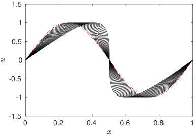
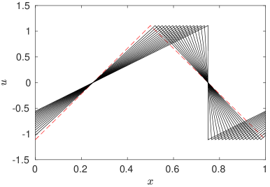
Figure 4: Solution of the inviscid Burgers equation (4) with (a) the unimodal initial condition (9) and (b) the extreme initial condition (11) for increasing times $t\in[0,t^{*}]$. The initial conditions are marked with red dashed lines and the solutions develop progressively steeper fronts as the time increases.

  

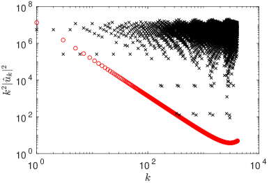
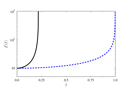
Figure 5: (a) Compensated Fourier spectra in the solution of the inviscid Burgers equation (4) with the extreme initial condition (11) at (red circles) the initial time $t=0$ and (black crosses) the blow-up time $t^{*}$. (b) The time history of the enstrophy ${\mathcal{E}}(t)$ in the solution of the inviscid Burgers equation (4) with (blue dashed line) the unimodal initial condition (9) and (black solid line) the extreme initial condition (11); in both cases the constant $A$ is chosen such that ${\mathcal{E}}(0)=\pi^{2}$.

The evolution of the viscous Burgers flow with the extreme initial condition $\widetilde{u}_{0;{\mathcal{E}}_{0}}$ shown in the physical space in figure 6(b) is qualitatively similar to the inviscid case, cf. figure 4(b), except that a singularity does not form. This behaviour is reflected in the spectrum of the solution which at all times $t>0$ decays exponentially for large wavenumbers $k$ (see figure 7(a)) and in the fact that the corresponding enstrophy ${\mathcal{E}}(t)$ starts to decrease after attaining a maximum at $t=\widetilde{T}_{{\mathcal{E}}_{0}}$ (see figure 7(b)). In figure 7(a) we also observe that, as expected (Bec & Khanin, 2007), for intermediate wavenumbers $k$ the Fourier spectrum scales as $|\widehat{u}_{k}(t)|\sim k^{-1}$, $t>0$. As regards the viscous Burgers flow corresponding to the generic initial condition shown in the physical space in figure 6(a), we observe that while a steep front is still formed, the maximum attained enstrophy is smaller than in the flow with the extreme initial condition $\widetilde{u}_{0;{\mathcal{E}}_{0}}$ (see figure 7(b)). The “irregular” behaviour of the solution apparent in figure 6(a) is due to the random form of the generic initial condition (cf. § 2.3).

  

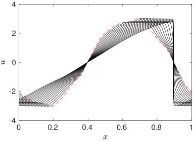
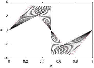
Figure 6: Solution of the viscous Burgers equation (3) with the (a) generic and (b) extreme initial condition $\widetilde{u}_{0;{\mathcal{E}}_{0}}$ for increasing times $t\in[0,1.25\,\widetilde{T}_{{\mathcal{E}}_{0}}]$. The initial conditions are marked with red dashed lines and the solutions develop progressively steeper fronts as the time increases.

  

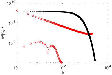
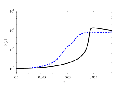
Figure 7: (a) Compensated Fourier spectra in the solution of the viscous Burgers equation (3) with the extreme initial condition $\widetilde{u}_{0;{\mathcal{E}}_{0}}$ at (red circles) the initial time $t=0$ and (black crosses) the time $\widetilde{T}_{{\mathcal{E}}_{0}}$ when the largest enstrophy is achieved for ${\mathcal{E}}_{0}=100$. (b) The time history of the enstrophy ${\mathcal{E}}(t)$ in the the solution of the viscous Burgers equation (3) with (blue dashed line) the generic and (black solid line) extreme initial condition $\widetilde{u}_{0;{\mathcal{E}}_{0}}$.

We now go on to analyze these flows in terms of the diagnostics focusing on fluxes and triad interactions introduced in § 3.1. We begin by noting in figure 10 that the solutions of the inviscid Burgers system (4) with the unimodal and extreme initial conditions (9) and (11) exhibit only forward energy cascade with non-negative flux $\Pi(t,k)\geq 0$ at all times $t$ and for all wavenumbers $k$. In the flow corresponding to the unimodal initial data (9) the flux $\Pi(t,k)$ is essentially independent of the wavenumber $k$ and rapidly increases from a small initial value to a nearly constant level. The small initial values of the flux and its independence of the wavenumber can be attributed to the fact that the unimodal initial condition (9) contains a single Fourier component only. On the other hand, for the extreme initial data (11) the flux is an increasing function of the wavenumber $k$ at early times $t$. Moreover, in this case the flux $\Pi(t,k)$ increases more rapidly with time and reaches larger values as the blow-up time $t^{*}$ is approached.

The PDFs of triad phases $\varphi_{k_{1},k_{2}}^{k_{3}}$ in inviscid Burgers flows are shown in figure 10. We notice that in the flows corresponding to both the unimodal and extreme initial conditions (9) and (11) a significant fraction of these phases is aligned at the angle $-\pi/2$, which in the light of formula (17) indicates that these triads may provide negative contributions to the flux. In fact, in the solution corresponding to the extreme initial condition (11), alignment at $\pm\pi/2$ is close to being equally probable for times $t\ll t^{*}$, but all triad phases collapse at $\pi/2$ as $t\rightarrow t^{*}$, cf. figure 10(a). However, the weighted PDF presented in figure 10(a) indicates that the triads with phases aligned at $-\pi/2$ do not in fact participate in the energy transfer. The reason is that these triads involve modes with vanishing Fourier coefficients, such that their contributions to flux (17) is effectively zero. On the other hand, the weighted PDF for the flow with the extreme initial condition (11) provides evidence for inverse energy transfer occurring at the beginning of the flow evolution.

  

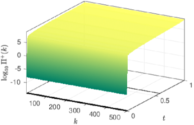
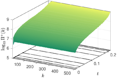
Figure 9: Time evolution of the PDF of the triad phase $\varphi_{k_{1},k_{2}}^{k_{3}}$ in the solution of the inviscid Burgers equation (4) with (a) the unimodal initial condition (9) and (b) the extreme initial condition (11) for $t\in[0,t^{*}]$.

Figure 10: Time evolution of the weighted PDF of the triad phase $\varphi_{k_{1},k_{2}}^{k_{3}}$ in the solution of the inviscid Burgers equation (4) with (a) the unimodal initial condition (9) and (b) the extreme initial condition (11) for $t\in[0,t^{*}]$.

Figure 8: Flux $\Pi(t,k)$ as function of the time $t\in[0,t^{*}]$ and the wavenumber $k$ in the solution of the inviscid Burgers equation (4) with (a) the unimodal initial condition (9) and (b) the extreme initial condition (11).

     

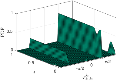
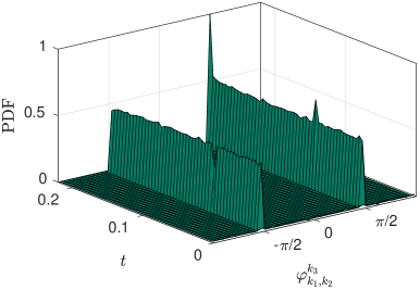
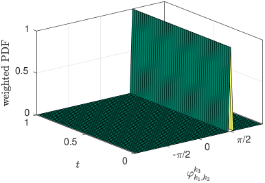
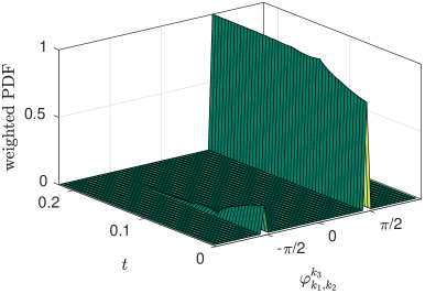
As regards solutions of the viscous Burgers system (3) with both the generic and extreme initial conditions, in figure 12 we note that the positive flux $\Pi^{+}(t,k)$ exhibits nontrivial behaviour. It becomes less intense at intermediate times and increases around the time $\widetilde{T}_{{\mathcal{E}}_{0}}$ when the maximum enstrophy is reached in both cases, at which point it also becomes almost independent of the wavenumber $k$. In the flow corresponding to the extreme initial condition the increase of the flux is more rapid which is also reflected in the steeper growth of enstrophy around that time, cf. figure 7(b). Interestingly, Figure 12 shows evidence of negative flux $\Pi^{-}(t,k)$ for small wavenumbers $k$ and at early times $t$ which is stronger in the flow with the extreme initial condition $\widetilde{u}_{0;{\mathcal{E}}_{0}}$. The time evolutions of the PDFs and the weighted PDFs of the triad phase angle $\varphi_{k_{1},k_{2}}^{k_{3}}$ in the solutions of the viscous Burgers system with the two initial conditions are overall similar to the inviscid cases, cf. figures 10 and 10 versus figures 14 and 14. One noteworthy difference is the virtual absence of triads with phases aligned at $-\pi/2$ in the viscous Burgers flow corresponding to the generic initial condition, cf. figure 14(a). Instead, triads initially exhibit a broad range of phase angles before suddenly aligning at $\pi/2$ which is accompanied by the emergence of a sharp front evident in figure 6(a). In addition, it is also interesting to note that in the solution of the viscous problem with the extreme initial condition $\widetilde{u}_{0;{\mathcal{E}}_{0}}$ all triad phases remain aligned at $\pi/2$ for $t>\widetilde{T}_{{\mathcal{E}}_{0}}$, i.e., after the enstrophy has reached its maximum, cf. figure 14(b). This mirrors the behaviour in the inviscid Burgers equation with the extreme initial condition, cf. figure 10(b).

     

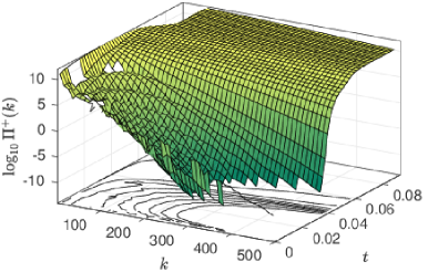
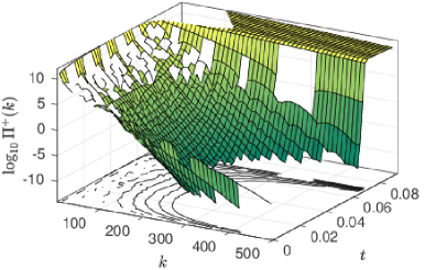
Figure 11: Positive flux $\Pi^{+}(t,k)$ as function of the time $t\in[0,1.25\,\widetilde{T}_{{\mathcal{E}}_{0}}]$ and the wavenumber $k$ in the solution of the viscous Burgers equation (3) with the (a) generic and (b) extreme initial condition $\widetilde{u}_{0;{\mathcal{E}}_{0}}$.

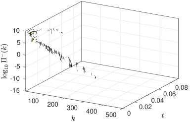
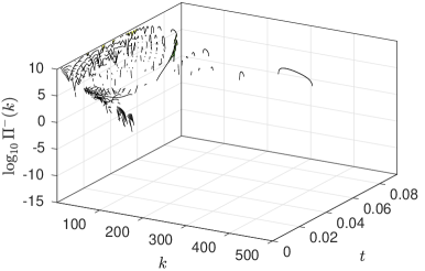
Figure 12: Negative flux $\Pi^{-}(t,k)$ as function of the time $t\in[0,1.25\,\widetilde{T}_{{\mathcal{E}}_{0}}]$ and the wavenumber $k$ in the solution of the viscous Burgers equation (3) with the (a) generic and (b) extreme initial condition $\widetilde{u}_{0;{\mathcal{E}}_{0}}$.

     

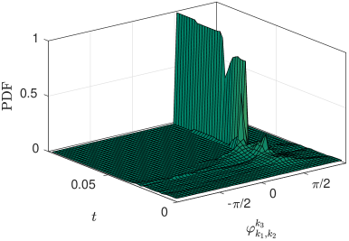
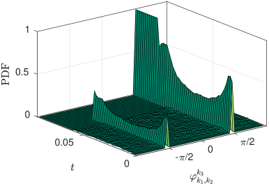
Figure 13: Time evolution of the PDF of the triad phase $\varphi_{k_{1},k_{2}}^{k_{3}}$ in the solution of the viscous Burgers equation (3) with the (a) generic and (b) extreme initial condition $\widetilde{u}_{0;{\mathcal{E}}_{0}}$.

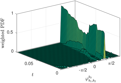
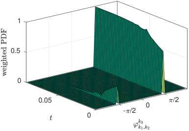
Figure 14: Time evolution of the weighted PDF of the triad phase $\varphi_{k_{1},k_{2}}^{k_{3}}$ in the solution of the viscous Burgers equation (3) with the (a) generic and (b) extreme initial condition $\widetilde{u}_{0;{\mathcal{E}}_{0}}$.

 

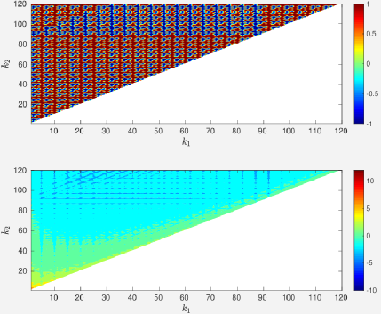
(a) $t_{1}=0.044$

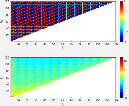
(b) $t_{2}=0.176$

Figure 15: Dependence of (top panels) $\sin\left(\varphi_{k_{1},k_{2}}^{k_{3}}\right)$ and (bottom panels) $\log_{10}\left(4\pi k_{1}\,{a}_{k_{1}}{a}_{k_{2}}{a}_{k_{3}}\right)$ on the wavenumbers $(k_{1},k_{2})$ at the indicated times $t_{i}\in(0,t^{*})$, $i=1,2,3,4$, during the evolution of the inviscid Burgers flow with the extreme initial condition (11). An animated version of this figure is available on-line.

 

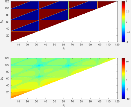
(c) $t_{3}=0.211$

(d) $t_{4}=0.224$

In order to provide additional interesting insights about the triadic interactions in the inviscid Burgers flow with the extreme initial condition (11), in figure 15(b) we show the quantity $\sin\left(\varphi_{k_{1},k_{2}}^{k_{3}}\right)$ and the logarithm of the corresponding amplitude-dependent factor $\log_{10}\left(4\pi k_{1}\,{a}_{k_{1}}{a}_{k_{2}}{a}_{k_{3}}\right)$, cf. (17), as functions of the wavenumbers $k_{1}$ and $k_{2}$ (where $k_{3}=-(k_{1}+k_{2})$) at different times $t\in(0,t^{*})$ (an animated version of this figure is available on-line). We note that the triads with phases aligned such that $\varphi_{k_{1},k_{2}}^{k_{3}}=\pm\frac{\pi}{2}$ exhibit an intriguing “triangular” pattern in the half plane $\{(k_{1},k_{2}),\ k_{1}\in{\mathbb{Z}}^{+},\ k_{2}\geq k_{1}\}$ as the blow-up time $t^{*}$ is approached (for better resolution, we have only shown the range $k_{1},k_{2}\in[1,120]$, however, the same pattern is also evident for larger values of the wavenumbers). More specifically, this pattern can be empirically described as

$$\forall k_{1}\in{\mathbb{Z}}^{+},\quad\varphi_{k_{1},k_{2}}^{k_{3}}(t)=\left\{\begin{aligned} &\frac{\pi}{2},&\quad&k_{2}\in\bigcup_{p=0}^{\infty}\left[k_{1}+p\kappa(t),\left\lfloor\frac{k_{1}}{\kappa(t)}\right\rfloor+(p+1)\kappa(t)\right]\\ -&\frac{\pi}{2},&&\text{otherwise}\end{aligned}\right.,$$ (35)

where the ”offset” $\kappa(t)\in{\mathbb{Z}}^{+}$ increases without bound as $t\rightarrow t^{*}$ (it can be interpreted as the length of the side of an elementary triangle in the pattern). This latter property signals an increasing synchronization of the triads as the blow-up time is approached. This pattern is also evident, albeit less pronounced due to a wider spread of values, in the corresponding flux contributions shown in the bottom panels in figure 15(b). We add that triad interactions in the viscous Burgers flow corresponding to the extreme initial data $\widetilde{u}_{0;{\mathcal{E}}_{0}}$ (not shown here) exhibit similar trends to those visible in figure 15(b). On the other hand, the inviscid Burgers flow with the unimodal initial condition (9) (also not shown here) reveals a nearly instantaneous synchronization with $\kappa(t)$ becoming unbounded very quickly, such that the distributions of $\sin\left(\varphi_{k_{1},k_{2}}^{k_{3}}\right)$ and $\log_{10}\left(4\pi k_{1}\,{a}_{k_{1}}{a}_{k_{2}}{a}_{k_{3}}\right)$ at all times $t\in(0,t^{*})$ resemble those in figure 15(b)(d). We remark that similar patterns have also been observed in viscous Burgers flows in the presence of stochastic forcing (Murray, 2017; Murray & Bustamante, 2018).

4.2 Results for 3D Navier-Stokes flows

We present the results for 3D Navier-Stokes flows by first briefly discussing classical diagnostics, namely, the time evolution of Fourier spectra, enstrophy and energy fluxes, applied to flows with the three initial conditions (extreme, generic and Taylor-Green, cf. § 2) before moving on to analyze these flows in terms of the diagnostics based on the triad interactions introduced in § 3.2. Figure 16(a) shows the initial ($t=0$) and final ($t=\widetilde{T}_{{\mathcal{E}}_{0}}$) energy spectra (23) for the three initial conditions. As for the initial spectra, the extreme case has a distribution across a range of wavenumbers and the spectrum of the initial condition in the generic case is by definition identical. On the other hand, the initial spectrum in the Taylor-Green case has energy concentrated in a small subset only of low wavenumbers. As for the final spectra, in all cases the energy has been transferred to higher wavenumbers, with the Taylor-Green case showing a less dramatic transfer to high wavenumbers; the extreme and generic cases look quite similar, but the extreme case shows slightly larger transfers to high wavenumbers. However, none of these energy spectra exhibits a wide inertial range which is due to a relatively low Reynolds number. It is evident from a comparison with the $k^{-5/3}$ line in figure 16(a) that an inertial range spans the wavenumbers $k=1$ to $k=3$, while a dissipative range involves wavenumbers $k\geq 10$ (this will be further justified by analysis of the fluxes shown in figure 20). The helicity spectra for the three types of flows considered are identically zero due to the fact that the flows are odd under the parity transformation. Figure 16(b) shows the time evolution of the total enstrophy for each of the three cases. It is evident that the Taylor-Green case shows a modest only growth of enstrophy, while the generic case is quite close to the extreme case.

  

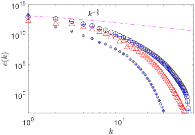
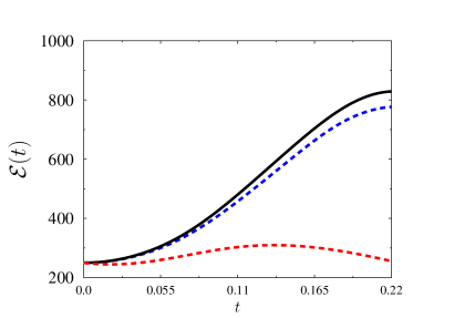
Figure 16: (a) Energy spectra (23) of the solution of the Navier-Stokes equation (1) with the extreme initial condition (black circles), the generic initial condition (blue crosses) and the Taylor-Green initial condition (red triangles) at the initial time $t=0$ (small symbols) and the time $t=\widetilde{T}_{{\mathcal{E}}_{0}}$ (large symbols) when the largest enstrophy is achieved for ${\mathcal{E}}_{0}=250$. The straight line represents the expression $k^{-5/3}$. (b) The time history of the enstrophy ${\mathcal{E}}(t)$ in the solution of the Navier-Stokes equation (1) with the extreme initial condition (black solid line), the generic initial condition (blue dashed line) and the Taylor-Green initial condition (red dashed line) for ${\mathcal{E}}_{0}=250$.

We now discuss the time evolution of the energy flux in the flows with the three initial conditions considered. In each case the spectral flux of energy is evaluated as

$$\Pi(t,k):=\Pi_{{\mathcal{C}}_{k}}(t),\qquad{\mathcal{C}}_{k}=\{\mathbf{k}\in\mathbb{Z}^{3}\setminus\{0\}\quad|\quad|\mathbf{k}|>k\}\,,$$ (36)

where $\Pi_{{\mathcal{C}}}$ is defined in its basic form in equation (25). To separate positive and negative contributions representing, respectively, the direct and inverse energy cascades, we decompose the flux as $\Pi(t,k)=\Pi^{+}(t,k)-\Pi^{-}(t,k)$, where $\Pi^{+}(t,k),\Pi^{-}(t,k)\geq 0$ and $\Pi^{+}(t,k)\Pi^{-}(t,k)=0$ for all wavenumbers $k$ and times $t$. These quantities are plotted in figures 19, 19 and 19 for the extreme, generic and Taylor-Green case. We remark that for practical reasons the data in these plots is obtained directly by evaluating the nonlinear term in the Fourier representation of the Navier-Stokes equation (1a) rather than by computing the sums in (25).

     

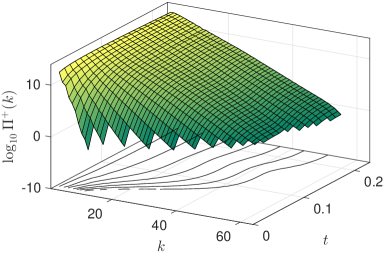
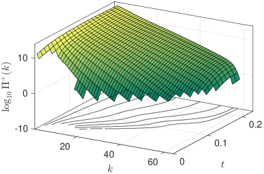
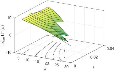
Figure 17: [Extreme case:] (a) Positive and (b) negative part of flux $\Pi(t,k)$ as function of the time $t\in[0,\widetilde{T}_{{\mathcal{E}}_{0}}]$ and the wavenumber $k$ in the solution of the Navier-Stokes equation with the indicated initial condition. Contours in the $(t,k)$ plane are the level sets of $\Pi^{+}(t,k)$ and $\Pi^{-}(t,k)$ corresponding to the values $10^{0},10^{2},\dots,10^{12}$.

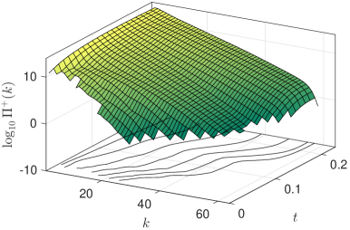
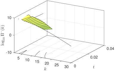
Figure 18: [Generic case:] See the caption of figure 19 for details.

Figure 19: [Taylor-Green case:] Positive part of flux $\Pi(t,k)$ as function of the time $t\in[0,{\widetilde{T}_{{\mathcal{E}}_{0}}}]$ and the wavenumber $k$ in the solution of the Navier-Stokes equation with the Taylor-Green initial condition. The negative part of flux $\Pi(t,k)$ vanishes for the Taylor-Green case. Contours in the $(t,k)$ plane are the level sets of $\Pi^{+}(t,k)$ corresponding to the values $10^{0},10^{2},\dots,10^{12}$.

Figures 19(a) and 19(b) show, respectively, positive and negative fluxes for the case of the extreme initial condition. It is evident that at early times there is a coherent negative flux at small wavenumbers. For a fixed time $t$, closely packed level sets represent a strong dependence on the wavenumber $k$. It is evident that, as the time approaches the end of the time window, the level sets become more spread out which corresponds to fluxes shifting towards larger wavenumbers $k$ and to a tendency towards a uniform flux.

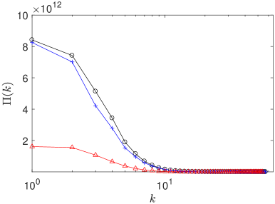
Figure 20: Flux $\Pi(k)$ as a function of the wavenumber $k$ at the final time $t=\widetilde{T}_{{\mathcal{E}}_{0}}$ in the solution of the Navier-Stokes equation (1) with the extreme initial condition (black circles), the generic initial condition (blue crosses) and the Taylor-Green initial condition (red triangles).

In a similar way, figures 19(a) and 19(b) show, respectively, positive and negative fluxes for the case of the generic initial condition. While the behaviour of the fluxes in this case appears similar to the extreme case, there are several differences of quantitative and qualitative nature. Comparing the negative flux contributions in figures 19(b) and 19(b), it is evident that while both cases initially show negative flux at small wavenumbers, this flux is short-lived in the generic case. Comparing now the positive flux contributions in figures 19(a) and 19(a), we see that initially the contours are more spread out in the generic case. This is solely due to the randomization of the phases of the generic initial condition, cf. § 2.3, which takes away the coherence required to obtain localized fluxes. Second, the dependence of the flux level sets on time is more erratic in the generic case, while in the extreme case there is a clear coherent shift of the level sets towards large wavenumbers.

Figure 19 shows the positive fluxes for the case of the Taylor-Green initial conditions (there are no negative fluxes in this case). One observes a rapid initial spreading of the level sets, mainly due to the fact that the Taylor-Green initial condition has its energy concentrated at small wavenumbers. After this initial phase, an intermediate regime occurs characterized by a quasi-steady state where the level sets change very little in time. Then, a final growth phase occurs which is however much milder than in the previous two cases. This can be inferred from the facts that: (i) the level set representing the smallest flux values reaches a lower wavenumber, and (ii) the level sets are less spread out at the end of the time window.

From a comparison of the time evolution of the positive fluxes for all cases, cf. figures 19(a), 19(a) and 19, we notice that both the generic and Taylor-Green cases display clear periods of stagnation in the time evolution of the level sets corresponding to large wavenumbers. They occur at intermediate times $t=0.75$–$0.125$ in the generic case and $t=0.1$–$0.15$ in the Taylor-Green case. This is another piece of evidence for the irregularity of the flux evolution across wavenumbers in these cases: when flux is steady (instead of growing in time) near a certain wavenumber $k_{0}$, there is more time for the energy to dissipate before it can flow to small scales. In contrast, the extreme case shows a smooth flux evolution across wavenumbers, without stagnation, which seems to facilitate the late-time maximization of the enstrophy.

The fluxes at the final time $t=\widetilde{T}_{{\mathcal{E}}_{0}}$ are compared between the three cases in figure 20 which confirms that the flux in the flow with the extreme initial condition is the most intense for all values of $k$ with the flux in the flow with the generic initial condition being only slightly smaller. The flux in the flow with the Taylor-Green initial condition is much weaker, approximately by a factor of four. The plots of flux in figure 20 confirm our earlier assessment (cf. figure 16) that an inertial range is found between wavenumbers $k=1$ and $k=3$ while a dissipative range is found for wavenumbers $k\geq 10$, as there is only about $1\%$ of the original flux left at that latter scale. More quantitatively, the Kolmogorov length scale can be estimated via $\eta:=(\nu^{3}/2\nu\mathcal{E}_{0})^{1/4}$, with $\nu=0.01$ and $\mathcal{E}_{0}=250$, giving $\eta\approx 0.02115$, and in terms of wavenumbers, $k_{\eta}:=2\pi/\eta\approx 297=3.48k_{\max}$. Thus, at $k=10$ we get a ratio $k_{\eta}/k\lessapprox 30$ which can be considered in the dissipative range.

We now proceed to discuss the flows considered in terms of the diagnostics based on the triad interactions introduced in § 3.2. With reference to the fluxes towards small spatial scales shown in figures 19, 19 and 19, we choose two representative cases: (i) fluxes towards the wavenumber region with $k>2$ corresponding to the inertial range of wavenumbers, i.e., those wavenumbers where energy is flowing due to nonlinear interactions and energy dissipation is negligible; (ii) fluxes towards the wavenumber region with $k>10$ corresponding to the dissipative range of wavenumbers, i.e., those wavenumbers where energy is still flowing due to nonlinear interactions but energy dissipation dominates, with a significant proportion of the energy having already been dissipated along the way from $k=2$ to $k=10$. We begin with the extreme case and in figure 21 show the time evolution of the PDFs $P_{\mathcal{C}_{2}}^{s_{1}s_{2}s_{3}}(\Phi)$ of the generalized helical triad phases participating in the fluxes out of the sphere defined in the spectral space by $k=2$, separately for each triad type $(s_{1}s_{2}s_{3})$. These results should be viewed with reference to equation (30) providing an expression for $\Pi_{\mathcal{C}}^{s_{1}s_{2}s_{3}}$ which is the contribution of triads of type $(s_{1}s_{2}s_{3})$ to the spectral energy flux into a set $\mathcal{C}$, here defined as $\mathcal{C}=\mathcal{C}_{2}=\{\mathbf{k}\in\mathbb{Z}^{3}\setminus\{0\}\quad|\quad|\mathbf{k}|>2\}$. The figure shows the time evolution of the PDFs ${\mathcal{P}}_{\mathcal{C}_{2}}^{s_{1}s_{2}s_{3}}(\Phi)$ of four selected generalized helical triad types, namely, the ones which exhibit variability of at least $\pm 5\%$ with respect to the uniform distribution equal to $1/2\pi(\approx 0.16)$: $(s_{1},s_{2},s_{3})=$ PPP, PMM, P(PM), (PM)P, where the last two triad types are of the boundary types, corresponding to the restrictions $|\mathbf{k}_{1}|=|\mathbf{k}_{2}|$ and $|\mathbf{k}_{2}|=|\mathbf{k}_{3}|$, respectively. For these triad types the PDFs vary slightly over the range from about $0.14$ to $0.18$, cf. table 3, third column. The only exception (and a quite remarkable one) is the case of the boundary triad type (PM)P whose PDF varies from about $0$ to $0.62$ (table 3, third column and bottom row) and is clearly concentrated near $\Phi=0$ (figure 21(d)). However, as figure 21 shows clearly, at later times the PDFs change. The most active one is again the boundary triad of type (PM)P, whose PDF exhibits a coherent behaviour over time, with some local maxima oscillating about $\Phi=0$ and other local maxima oscillating about $\Phi\approx\pm 3\pi/4$. Also active are the triad types PPP and PMM whose PDFs reveal a persistent late-time preference for values near $\pi$ or $-\pi$ (figure 21(a)–(b)). As explained in the text preceding equation (29), triad phases with values near $0$ give rise to positive contributions to the flux, whereas values near $\pm\pi$ produce negative contributions to the flux. In the light of this alone, it might appear from these figures that contributions to the flux from individual triads have mixed signs, and thus the total contribution to the flux may change sign as a function of time. However, one has to bear in mind that contributions to the flux also depend on mode amplitudes which are constantly changing as well.

	Fraction for $k=2$	Fraction for $k=10$
PPP	$24.944\%$	$24.986\%$
PPM	$24.944\%$	$24.986\%$
PMP	$24.944\%$	$24.986\%$
PMM	$24.944\%$	$24.986\%$
P(PM)	$0.224\%$	$0.054\%$
(PM)P	$9.48\times 10^{-5}\%$	$1.03\times 10^{-3}\%$

Table 2: Proportion of triads of different types participating in energy flux to regions ${\mathcal{C}}_{k}$ in the wavenumber space, cf. (36), with the indicated radii $k$. These fractions are functions of $k$ only and do not depend on the initial condition.

	$k=2$, PDF	$k=2$, wPDF	$k=10$, PDF	$k=10$, wPDF
PPP	[0.145,0.176]	[0.016,0.617]	[0.158,0.161]	[0.068,0.561]
PPM	[0.158,0.161]	[0.025,0.485]	[0.159,0.160]	[0.086,0.355]
PMP	[0.156,0.162]	[0.019,0.732]	[0.159,0.160]	$[0.100,0.283]$
PMM	[0.148,0.171]	[0.008,0.780]	[0.157,0.162]	$[0.066,0.555]$
P(PM)	[0.150,0.167]	[0.001,0.632]	[0.158,0.161]	$[0.027,0.577]$
(PM)P	[0.000,0.620]	[0.000,1.537]	[0.150,0.170]	$[0.040,0.550]$

Table 3: [Extreme case:] Upper and lower bounds on the PDFs and wPDFs of triad phases of the different types in the Navier-Stokes flow with the extreme initial data, cf. figures 21–25. Shaded intervals (light gray) represent PDFs that are very close (within $\pm 5\%$) to the uniform distribution $1/2\pi\approx 0.16$.

     

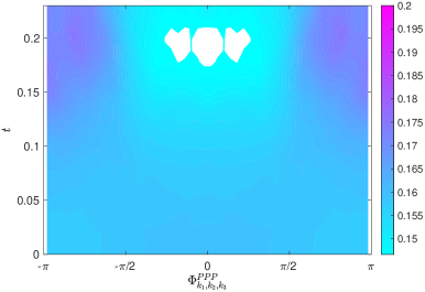
(a) ${\mathcal{P}}_{\mathcal{C}_{2}}^{PPP}(\Phi)(t)$

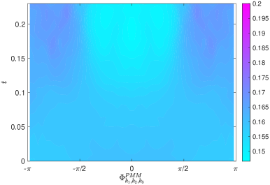
(b) ${\mathcal{P}}_{\mathcal{C}_{2}}^{PMM}(\Phi)(t)$

(c) ${\mathcal{P}}_{\mathcal{C}_{2}}^{P(PM)}(\Phi)(t)$

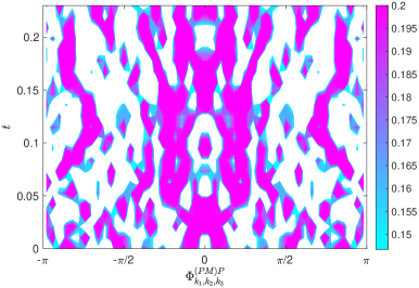
(d) ${\mathcal{P}}_{\mathcal{C}_{2}}^{(PM)P}(\Phi)(t)$

Figure 21: [Extreme case, $k>2$:] Time evolution of the PDFs of the triad phase angle ${\mathcal{P}}_{\mathcal{C}_{2}}^{s_{1}s_{2}s_{3}}(\Phi)$ for triads of different types in the Navier-Stokes flow with the extreme initial data. Only triad types with PDFs revealing variability of at least $\pm 5\%$ with respect to the uniform distribution $1/2\pi\approx 0.16$ (corresponding to light blue color in the plots), are shown: (a) “PPP”, (b) “PMM”, (c) “P(PM)” and (d) “(PM)P”.

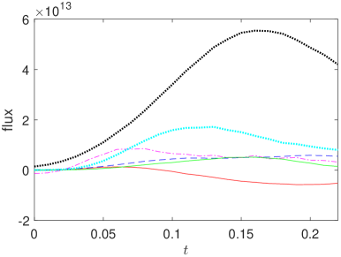
(a) Extreme case: Flux towards $k>2$

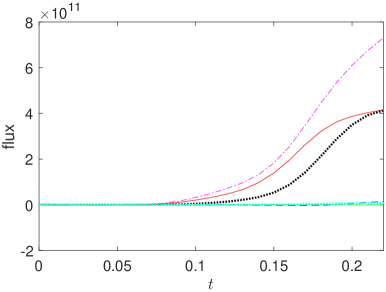
(b) Extreme case: Flux towards $k>10$

Figure 22: Time evolution of the fluxes towards $\mathcal{C}_{2}$ ($k>2$) (left panels (a), (c) and (e)) and $\mathcal{C}_{10}$ ($k>10$) (right panels (b), (d) and (f)) in the solution of the Navier-Stokes system with the extreme initial condition (top panels (a) and (b)), generic initial condition (middle panels (c) and (d)) and Taylor-Green initial condition (bottom panels (e) and (f)) contributed by the different triad types: “PPP” (red solid line), “PPM” (blue dashed line), “PMP” (black dotted line), “PMM” (magenta dash-dotted line), “P(PM)” (green solid line), and “(PM)P ” (cyan dotted line).

     

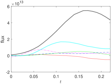
(c) Generic case: Flux towards $k>2$

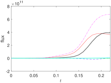
(d) Generic case: Flux towards $k>10$

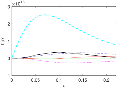
(e) Taylor-Green case: Flux towards $k>2$

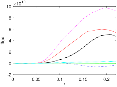
(f) Taylor-Green case: Flux towards $k>10$

For the above reason we need to look at the positive-definite flux densities $F_{\mathcal{C}_{2}}^{s_{1}s_{2}s_{3}}(\Phi)$ constructed in terms of the contribution to the flux $\Pi_{\mathcal{C}_{2}}^{s_{1}s_{2}s_{3}}$ from generalized helical triad phases $\Phi_{\mathbf{k}_{1}\mathbf{k}_{2}\mathbf{k}_{3}}^{s_{1}s_{2}s_{3}}$ with values $\Phi$, cf. relation (33). The plot of these fluxes $\Pi_{\mathcal{C}_{2}}^{s_{1}s_{2}s_{3}}$ as functions of time for each helical triad type is shown in figure 22(b)(a). It is evident from this plot that there is an early energy transfer out of the sphere defined by $k=2$ due to the PMP triad type, which is the main contributor to the flux having a maximum flux at a relatively late time ($t\approx 0.17$). The second most important contributor to the positive flux is the boundary triad type (PM)P, whose contribution is comparable to the one from the PMP triads (somewhat surprisingly as the number of (PM)P triads is relatively small), but has an earlier maximum flux, at about $t\approx 0.11$. The third contributor in importance is the PMM triad type, with a less significant contribution to the positive flux except for early times, with a maximum at about $t\approx 0.06$. A notable feature of this PMM triad type is the evidence of an initially negative contribution, which nevertheless does not show up in the negative flux plot in figure 19(b) as the total flux is positive once the contribution from the PMP triad type is added.

Having established that the different triad types exhibit different time dynamics, we now analyze the detailed phase dependence of the normalized flux densities ${\mathcal{W}}_{\mathcal{C}_{2}}^{s_{1}s_{2}s_{3}}(\Phi)$, cf. expression (34), which are shown in figure 23 for the six helical triad types. The fact that these plots provide, at any given time, normalized distributions, is useful for the purpose of detecting phase coherence and complements the flux plots in figure 22(b)(a): in fact, the normalizing factors above can be reconstructed from these complementary figures. A striking coherent pattern emerges, showing for the first time the evolution of the structure of the flux-carrying helical triads during an extreme event occurring in the forward energy cascade. Qualitatively, a remarkable feature characterizing all the six helical triad types is that salient peaks of the weighted PDFs (darker, redder colours) seem to propagate in time in a continuous manner, revealing distinctive braid patterns which suggest that the sets of flux-carrying helical triads slowly change over time. Although we will not attempt a thorough classification of these sets, the case of the (PM)P boundary helical triad gives a clue for a quantitative analysis. There, the weighted PDF (figure 23(f)) shows a clear and persistent concentration in the positive-flux range $-\pi/2<\Phi<\pi/2$, near the time of its maximum flux ($t\approx 0.11$), and it is evident that these peaks are well correlated with the peaks in the PDF (figure 21(d)), leading to the conclusion that the majority of the triads in this helical triad type contribute actively to the flux. Although these (PM)P triads represent less than the $0.0001\%$ of all triads participating in the flux towards modes with $k>2$, they contribute with over $20\%$ of the total flux at $t\approx 0.11$ (these numbers can be calculated from an assessment of the number of triads in table 3 (second column) and from the flux plot in figure 22(b)(a)). The preference for positive flux contributions is also evident for other triad types. Figure 23(d) shows, for the PMM triad type, the strongest concentration of the weighted PDF at positive-flux phases $\Phi\approx\pm 0.25\pi$, near the time of its maximum flux ($t\approx 0.06$). Finally, the weighted PDF for the main contributor to the positive flux (triad type PMP, figure 23(c)) shows strong local maxima near $\Phi=0$ at times $t\approx 0.06$ and $t\approx 0.11$, while a set of weaker local maxima at positive-flux phases $\Phi\approx\pm 0.1\pi$ occurs at the time of the maximum flux ($t\approx 0.17$). This latter case demonstrates how important it is to complement the flux plots in figure 22(b)(a) with the weighted PDF plots in figure 21 as the former plots do not contain information about the flux densities for different triad types. Even negative-flux contributions can be identified by these analyses. Figure 23(a) shows, for the PPP triad type, a late-time preference for negative-flux contributions (weighted PDF concentrated near $\Phi=\pm\pi$), which is evidenced in the plot of the total PPP flux in figure 22(b)(a), solid red line.

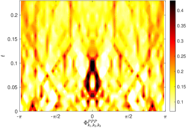
(a) ${\mathcal{W}}_{\mathcal{C}_{2}}^{PPP}(\Phi)(t)$

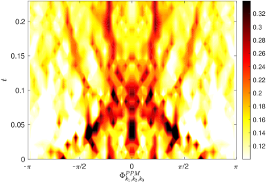
(b) ${\mathcal{W}}_{\mathcal{C}_{2}}^{PPM}(\Phi)(t)$

     

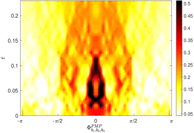
(c) ${\mathcal{W}}_{\mathcal{C}_{2}}^{PMP}(\Phi)(t)$

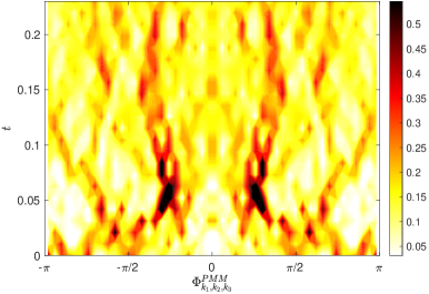
(d) ${\mathcal{W}}_{\mathcal{C}_{2}}^{PMM}(\Phi)(t)$

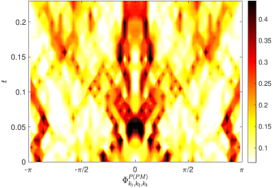
(e) ${\mathcal{W}}_{\mathcal{C}_{2}}^{P(PM)}(\Phi)(t)$

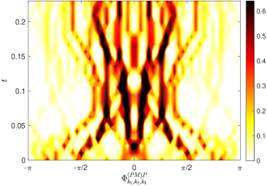
(f) ${\mathcal{W}}_{\mathcal{C}_{2}}^{(PM)P}(\Phi)(t)$

Figure 23: [Extreme case, $k>2$:] Time evolution of the weighted PDF of the triad phase angle ${\mathcal{W}}_{\mathcal{C}_{2}}^{s_{1}s_{2}s_{3}}(\Phi)$, cf. expression (34), in the Navier-Stokes flow with the extreme initial data for the triad types (a) “PPP”, (b) “PPM”, (c) “PMP” , (d) “PMM”, (e) “P(PM)” and (f) “(PM)P”. In these plots the uniform distribution corresponding to $1/2\pi\approx 0.16$ is depicted by yellow ($25\%$ of the colour bars).

In order to obtain a better idea of how the energy leaving the sphere $k=2$ is transported after reaching the dissipative range, we now perform an analogous study to the one just described, but this time regarding the energy flux out of the sphere $k=10$, namely towards the set $\mathcal{C}_{10}=\{\mathbf{k}\in\mathbb{Z}^{3}\setminus\{0\}\quad|\quad|\mathbf{k}|>10\}$. Table 3 (sixth column) shows that there is only one helical triad type — the boundary triad (PM)P — with a non-uniform PDF over the time window considered, cf. figure 24(a). In contrast, when we consider the flux densities and the corresponding weighted PDFs $W_{\mathcal{C}_{10}}^{s_{1}s_{2}s_{3}}(\Phi)$, cf. relations (33) and (34), shown in figure 25, clear coherent patterns emerge, although they are not as sustained over time as in the case with $k>2$; rather, they typically consist of an initial burst of concentrated coherent flux followed by a more disperse tail. Again, for a complete picture, these are to be complemented with plots of the fluxes $\Pi_{\mathcal{C}_{10}}^{s_{1}s_{2}s_{3}}$ shown in figure 22(b)(b): now, the main contributor to the flux towards $\mathcal{C}_{10}$ is triad type PMM, followed by PPP and PMP. The plot shows that a stage of sustained growth begins at around $t=0.075$. Could this growth stage be related to the coherent patterns observed in figure 25? Possibly yes, as coherent patterns develop near that time among positive-flux phases, leading to a build-up of energy over time. As for the main contributor to the energy flux, namely the set of PMM helical triads, its weighted PDF is shown in figure 25(d), revealing a strong and coherent event near $\Phi\approx\pm 0.075\pi$ which occurs during $t=0.04$–$0.1$ and retains coherence after that. As for the second main contributor, the set of PPP helical triads, its weighted PDF in figure 25(a) shows a similar, even more concentrated, pattern near $\Phi=0$ during the same time range. Notably, the weighted PDFs of both these triad types show early coherence ($t=0$–$0.03$) at triad phases corresponding to negative flux contributions. At these early stages the actual fluxes are quite small so one could conjecture that a kind of “slingshot effect” is at work for this extreme initial condition, similarly to the extreme initial condition in the Burgers case, where an initial stage of negative-flux phase alignments (triad phases near $-\pi/2$ in the Burgers case, and near $\pi$ or $-\pi$ in the Navier-Stokes case) is followed by a rearrangement of the phases to favor forward energy cascade (triad phases near $\pi/2$ in the Burgers case, and near $0$ in the Navier-Stokes case). As for the third contributor to the flux, the set of PMP helical triads, its weighted PDF in figure 25(c) shows a clear initial positive-flux concentration near $\Phi=0$, followed by a dip to a close-to-uniform distribution at $t=0.04$, leading to another event when the positive flux attains local maxima in the range $t=0.04-0.1$, to then become gradually less concentrated for the rest of the time window.

  

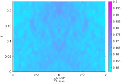
(a) ${\mathcal{P}}_{\mathcal{C}_{10}}^{(PM)P}(\Phi)(t)$ (extreme)

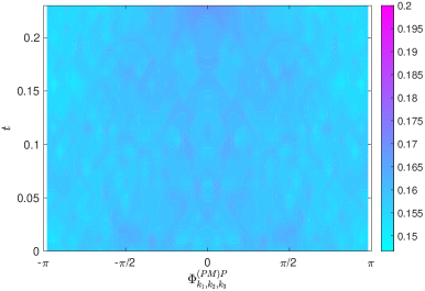
(b) ${\mathcal{P}}_{\mathcal{C}_{10}}^{(PM)P}(\Phi)(t)$ (generic)

(c) ${\mathcal{P}}_{\mathcal{C}_{10}}^{(PM)P}(\Phi)(t)$ (Taylor-Green)

Figure 24: [$k>10$:] Time evolution of the PDFs of the phase triad angle ${\mathcal{P}}_{\mathcal{C}_{10}}^{(PM)P}(\Phi)$ in the solution of the Navier-Stokes system with the (a) extreme, (b) generic, and (c) Taylor-Green initial conditions. The “(PM)P” triad is the only triad type exhibiting a PDF with variability exceeding $\pm 5\%$ with respect to the uniform distribution equal to $1/2\pi$ ($\approx 0.16$, which corresponds to light blue colour in the plots). The PDFs for all the other five triad types (“PPP”, “PPM”, “PMP”, “PMM” and “P(PM)”) are not shown, as they are essentially uniform (see tables 3, 4 and 5).

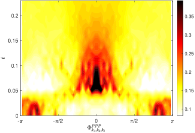
(a) ${\mathcal{W}}_{\mathcal{C}_{10}}^{PPP}(\Phi)(t)$

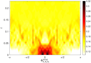
(b) ${\mathcal{W}}_{\mathcal{C}_{10}}^{PPM}(\Phi)(t)$

     

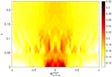
(c) ${\mathcal{W}}_{\mathcal{C}_{10}}^{PMP}(\Phi)(t)$

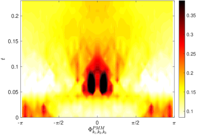
(d) ${\mathcal{W}}_{\mathcal{C}_{10}}^{PMM}(\Phi)(t)$

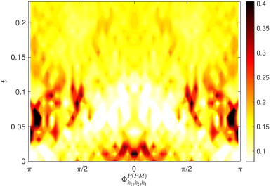
(e) ${\mathcal{W}}_{\mathcal{C}_{10}}^{P(PM)}(\Phi)(t)$

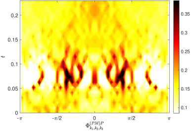
(f) ${\mathcal{W}}_{\mathcal{C}_{10}}^{(PM)P}(\Phi)(t)$

Figure 25: [Extreme case, $k>10$:] Time evolution of the weighted PDF of the triad phase angle ${\mathcal{W}}_{\mathcal{C}_{10}}^{s_{1}s_{2}s_{3}}(\Phi)$, cf. expression (34), in the Navier-Stokes flow with the extreme initial data for the triad types (a) “PPP”, (b) “PPM”, (c) “PMP” , (d) “PMM”, (e) “P(PM)” and (f) “(PM)P”. In these plots the uniform distribution corresponding to $1/2\pi\approx 0.16$ is depicted by yellow ($25\%$ of the colour bars).

We now turn to the case of the generic initial condition, cf. § 2.3, and compare the fluxes and triads analyses against the extreme case. Let us recall that in the generic case the initial amplitudes of the Fourier coefficients are the same as in the extreme case, while their phases are initially set as random variables with uniform distributions over $[0,2\pi)$. Therefore, the generic case offers a method to test whether or not the observed phase coherence in the extreme case is due to a special initial condition on the triad phases.

Interestingly, the results for the generic case are hardly distinguishable from those for the extreme case. To begin with, as regards the flux towards the wavenumber region $k>2$, table 4 (second column) shows again that the same four triad types as in the extreme case have PDFs with variability of $\pm 5\%$ or more with respect to the uniform case. Figure 26 shows these PDFs and it is evident that, apart from details, the generic case displays essentially the same global features as the extreme case, including the coherent patterns in panel (d) corresponding to (PM)P helical triads. Next, the time evolution of the fluxes for each of the six triad types towards the wavenumber region $k>2$ is plotted in figure 22(b)(c). Comparing this with the extreme case in figure 22(b)(a), it is evident that each triad type shows a similar trend, with small differences related to the timing and value of flux maxima. In particular, the (PM)P boundary triad type is again seen to contribute well over $20\%$ of the total flux near $t=0.11$, despite the fact that (PM)P triads constitute only less than $0.0001\%$ of the total number of triads participating in energy transfer. Again, the triad types that contribute the most to the flux are, in order of importance, PMP, (PM)P and PMM. The next piece of analysis concerns the weighted PDFs for the generic case shown in figure 27(b). A quick qualitative comparison with the extreme case, cf. figure 23, demonstrates the same overall patterns of coherence. Focusing now our attention on the main flux contributors: PMP in panel (c), (PM)P in panel (f) and PMM in panel (d), we clearly observe an early burst of positive flux at $t=0.05$ in the weighted PDF for the PMM triads, followed by a pronounced accumulation of the weighted PDF around $\Phi=0$ at $t=0.05$—$0.1$ and then another such event at $t=0.07$—$0.11$ for the (PM)P triads. This is qualitatively very similar to the extreme case. However, from the quantitative point of view, we can state that in the present case the three main flux contributors show a less extreme behaviour in their weighted PDFs: comparing the ranges of values of the weighted PDFs in the the extreme case (table 3, fourth column) with the same ranges for the generic case (table 4, third column) for the triad types PMP, (PM)P and PMM, it is evident that the range in the generic case is about 30% to 35% smaller than in the extreme case. This could be attributed to an initial lack of coherence in the phases, which translates into a less coherent time evolution.

	$k=2$, PDF	$k=2$, wPDF	$k=10$, PDF	$k=10$, wPDF
PPP	[0.145,0.171]	[0.022,0.770]	[0.158,0.161]	[0.039,0.898]
PPM	[0.157,0.161]	[0.031,0.497]	[0.159,0.160]	[0.089,0.361]
PMP	[0.156,0.162]	[0.033,0.537]	[0.159,0.160]	$[0.104,0.281]$
PMM	[0.148,0.169]	[0.016,0.505]	[0.157,0.162]	$[0.054,0.806]$
P(PM)	[0.148,0.168]	[0.002,0.747]	[0.158,0.160]	$[0.027,0.660]$
(PM)P	[0.000,0.424]	[0.000,1.103]	[0.149,0.169]	$[0.051,0.520]$

Table 4: [Generic case:] Upper and lower bounds on the PDFs and wPDFs of triad phases of the different types in the Navier-Stokes flow with the generic initial data, cf. figures 26–28. Shaded intervals (light gray) represent PDFs that are very close (within $\pm 5\%$) to the uniform distribution $1/2\pi\approx 0.16$.

     

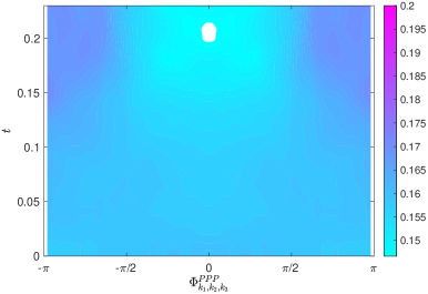
(a) ${\mathcal{P}}_{\mathcal{C}_{2}}^{PPP}(\Phi)(t)$

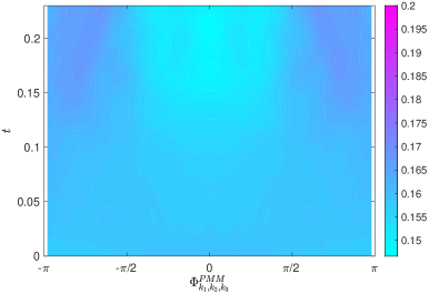
(b) ${\mathcal{P}}_{\mathcal{C}_{2}}^{PMM}(\Phi)(t)$

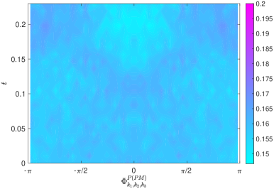
(c) ${\mathcal{P}}_{\mathcal{C}_{2}}^{P(PM)}(\Phi)(t)$

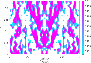
(d) ${\mathcal{P}}_{\mathcal{C}_{2}}^{(PM)P}(\Phi)(t)$

Figure 26: [Generic case, $k>2$:] Time evolution of the PDFs of the triad phase angle ${\mathcal{P}}_{\mathcal{C}_{2}}^{s_{1}s_{2}s_{3}}(\Phi)$ for triads of different types in the Navier-Stokes flow with the generic initial data. Only triad types with PDFs revealing variability of at least $\pm 5\%$ with respect to the uniform distribution $1/2\pi\approx 0.16$ (corresponding to light blue colour in the plots), are shown: (a) “PPP”, (b) “PMM”, (c) “P(PM)” and (d) “(PM)P”.

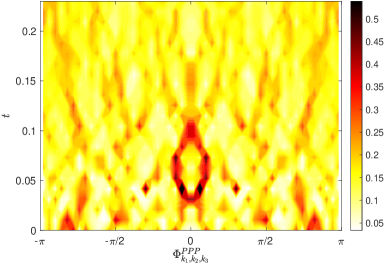
(a) ${\mathcal{W}}_{\mathcal{C}_{2}}^{PPP}(\Phi)(t)$

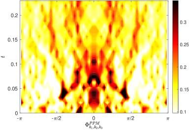
(b) ${\mathcal{W}}_{\mathcal{C}_{2}}^{PPM}(\Phi)(t)$

Figure 27: [Generic case, $k>2$:] Time evolution of the weighted PDF of the triad phase angle ${\mathcal{W}}_{\mathcal{C}_{2}}^{s_{1}s_{2}s_{3}}(\Phi)$, cf. expression (34), in the Navier-Stokes flow with the generic initial data for the triad types (a) “PPP”, (b) “PPM”, (c) “PMP” , (d) “PMM”, (e) “P(PM)” and (f) “(PM)P”. In these plots the uniform distribution corresponding to $1/2\pi\approx 0.16$ is depicted by yellow ($25\%$ of the colour bars).

     

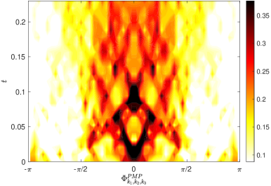
(c) ${\mathcal{W}}_{\mathcal{C}_{2}}^{PMP}(\Phi)(t)$

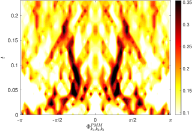
(d) ${\mathcal{W}}_{\mathcal{C}_{2}}^{PMM}(\Phi)(t)$

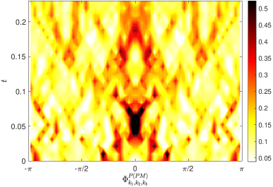
(e) ${\mathcal{W}}_{\mathcal{C}_{2}}^{P(PM)}(\Phi)(t)$

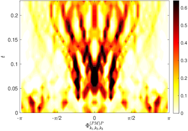
(f) ${\mathcal{W}}_{\mathcal{C}_{2}}^{(PM)P}(\Phi)(t)$

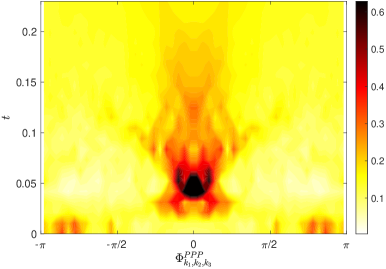
(a) ${\mathcal{W}}_{\mathcal{C}_{10}}^{PPP}(\Phi)(t)$

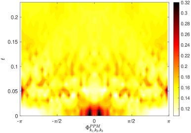
(b) ${\mathcal{W}}_{\mathcal{C}_{10}}^{PPM}(\Phi)(t)$

     

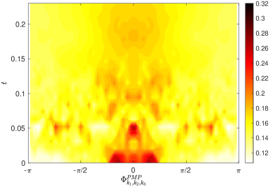
(c) ${\mathcal{W}}_{\mathcal{C}_{10}}^{PMP}(\Phi)(t)$

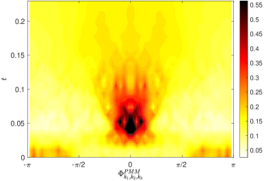
(d) ${\mathcal{W}}_{\mathcal{C}_{10}}^{PMM}(\Phi)(t)$

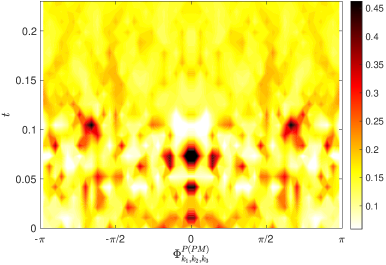
(e) ${\mathcal{W}}_{\mathcal{C}_{10}}^{P(PM)}(\Phi)(t)$

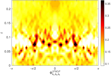
(f) ${\mathcal{W}}_{\mathcal{C}_{10}}^{(PM)P}(\Phi)(t)$

Figure 28: [Generic case, $k>10$:] Time evolution of the weighted PDF of the triad phase angle ${\mathcal{W}}_{\mathcal{C}_{10}}^{s_{1}s_{2}s_{3}}(\Phi)$, cf. expression (34), in the Navier-Stokes flow with the generic initial data for the triad types (a) “PPP”, (b) “PPM”, (c) “PMP” , (d) “PMM”, (e) “P(PM)” and (f) “(PM)P”. In these plots the uniform distribution corresponding to $1/2\pi\approx 0.16$ is depicted by yellow ($25\%$ of the colour bars).

Having shown that the generic and extreme cases display comparable behaviours in terms of the helical-triad assessment of the flux towards wavenumbers $k>2$, we now turn our attention to the corresponding study of the flux towards wavenumbers $k>10$. Firstly, we look at the time evolution of the fluxes for each triad type, shown in figure 22(b)(d) for the generic case. As in the extreme case, in the generic case the main contributors to the flux are, in order of importance, the triad types PMM, PPP and PMP. The time evolution of the fluxes for these triad types is qualitatively similar to the corresponding evolution in the extreme case, cf. figure 22(b)(d), with again small differences in the timing and values of the flux maxima. Importantly, in these plots it is always the case that a flux maximum is attained earlier in the generic case, with the extreme case attaining a higher value of the maximum flux. This difference of the timing and maximum value attained could be attributed to the lack of coherence in the generic case. Secondly, we assess the ranges of the weighted PDFs characterizing the main contributors to the flux. Comparing the range of values in the extreme case (table 3, last column) against those of the generic case (table 4, last column), we find that in contrast to the case with $k>2$, when $k>10$ it is the generic case that exhibits a broader range: for the PMM and PPP triads this range is about 50% to 70% larger than in the extreme case, while the range in the generic case for the PMP triads shows just a 3% reduction with respect to the extreme case. Does this contradict our earlier observations that the generic case is less coherent than the extreme case? Not necessarily, because even though the generic case shows a stronger coherence peak at early times, the extreme case is designed in order to maximize the late-time flux, cf. § 2.2. Comparing panels (b) and (d) of figure 22(b) and focusing on the main flux contributor—the PMM triads (magenta dash-dotted lines)—the extreme case indeed presents a slightly lower flux during early and intermediate times, but by the end of the time window the flux in the extreme case is larger and still growing, while in the generic case the flux is smaller and is already reaching a plateau.

A more detailed comparison between the generic and extreme cases regarding flux towards wavenumbers $k>10$ involves analyzing the weighted PDFs shown in figures 25 and 28 for the extreme and the generic case, respectively. Focusing on the main flux contributors—the triads PMM, PPP and PMP in panels (d), (a) and (c) of these figures—we see that the generic case exhibits stronger coherence peaks, but they occur earlier and are less sustained than in the extreme case. This is consistent with the analysis given in the preceding paragraph: while the generic case shows stronger phase coherence at early times, it fails to provide the delicate balance of phases required in order to sustain a large late-time flux. Maximizing this flux is what the extreme case is designed for.

Finally, we turn to the study of the flow corresponding to the Taylor-Green initial condition, cf. § 2.1, from the point of view of helical triads. In this case, the evolution is strikingly different from the extreme and generic cases. Let us recall that this initial condition contains Fourier components with only a few wavevectors, all with wavenumber $k=1$. Therefore, at the beginning it is expected to see low-dimensional dynamics confined to the low-wavenumber region. We first look at the flux towards the wavenumber region $k>2$. Data in table 5, second column, shows little difference with respect to the extreme and generic cases: again, only three triad types exhibit PDFs with variability of at least $\pm 5\%$ with respect to the uniform distribution, and again the (PM)P boundary triad type is the one showing the most variability. The PDFs of these three triad types are shown in figure 29. In comparison against the corresponding PDFs in the extreme and generic cases, here we see a clear difference regarding the (PM)P boundary triad type: on top of the typical coherent patterns also encountered in the other two cases, in the Taylor-Green case there is an extra band of densely populated phase values which persists throughout the time evolution. This band is clearly correlated with the band that dominates the weighted PDF for the (PM)P triad type shown in figure 30(f). Moreover, the actual flux contribution from the (PM)P triads, cf. figure 22(b)(e) (cyan dotted line), shows that this triad type contributes over $80\%$ of the total flux, while representing less than $0.0001\%$ of the total number of triads. Thus, we are led to the conclusion that the band structure of the PDFs and weighted PDFs is directly responsible for the observed robust flux behaviour for this triad type. Looking at the weighted PDFs of the four dominating triad types shown in figures 30(a–d), we again observe the presence of persistent bands, some of which seem to interact and evolve while keeping a strong coherence. However, the corresponding fluxes shown in figure 22(b)(e) are not particularly strong, suggesting that the coherence observed for these triad types is perhaps a secondary effect associated with their interaction with the flux-carrying (PM)P triads. At this stage it is relevant to note an important difference between the extreme and generic cases versus the Taylor-Green case evident in figures 22(b)(a,c,e): while both the extreme and the generic cases show a gradual development of their most important flux contributor, the triad type PMP, with a late-time maximum, the Taylor-Green case reveals an immediate growth of its most important flux contributor, the boundary triad type (PM)P, with an early-time maximum at half the strength as compared to the extreme and generic cases. Finally, a remarkable aspect of the flux to the wavenumber region $k>2$ in the Taylor-Green case is that the weighted PDF of the P(PM) triad type shown in figure 30(e) displays an extra symmetry about $\Phi=\pi/2$ (on top of the usual symmetry about $\Phi=0$), which implies that the flux contribution from this triad type is in fact identically zero. This extra symmetry could be related to a low effective dimension of the dynamical system associated with the Fourier modes with $k\leq 2$; the flux to the wavenumber region $k>10$, to be discussed next, does not exhibit this symmetry anymore.

We now discuss the flux towards wavenumbers $k>10$ in the flow with the Taylor-Green initial condition. Comparing the data in table 5, last two columns, with the corresponding columns for the other two cases in tables 3 and 4, we see no significant differences in the PDFs for all triad types. However, for the weighted PDFs, the Taylor-Green case displays a slightly larger range of values than in the extreme or generic cases for the four dominating triad types, while for the two boundary triad types, the range in the Taylor-Green case is several times larger than in the extreme or generic cases. Looking at the weighted PDFs for each triad type in figure 31, it is evident that the two boundary triad types show the band structure characteristic of the flux to wavenumbers $k>2$ discussed earlier. This band structure is responsible for an increased range in the weighted PDFs for these triad types as compared against the extreme and generic cases (however, as we shall see, in terms of total fluxes these triads do not contribute much). We also notice that the extra symmetry of the weighted PDF for the triad P(PM) is now broken. As for the four dominating triad types, cf. figure 31(a–d), these display a behaviour that is closer to the extreme and generic cases, in that the maxima of the weighted PDFs are more localized in time and the coherent patterns exhibit more complex dynamics, with no obviously persistent bands, a fact that is probably related to an increased number of degrees of freedom involved in the flux towards modes with wavenumbers $k>10$. An important difference with respect to the extreme and generic cases is that local maxima appear in the weighted PDFs at early times ($t=0.01$—$0.05$). This is further reflected in the evolution of the total flux shown in figure 22(b)(f) which reveals an early growth phase of the fluxes (starting at about $t=0.05$), much earlier than in the extreme and generic cases shown in figures 22(b)(b,d). These figures also show that the flux towards modes with wavenumbers $k>10$ for each triad type in the Taylor-Green case attains maxima at earlier times with peak values about $7$ times smaller than in the corresponding fluxes in the extreme and generic cases. Perhaps the only obvious similarity we could infer from a comparison of the three cases in figures 22(b)(b,d,f) is that the three dominating flux contributors are the same in these cases, namely, PMM, then PPP, followed by the PMP helical triads, with similar peak ratios. Another similarity—looking at the same figures—is that the three cases show a small negative flux contribution from the PPM triads near the end of the time window. This is also evident from the weighted PDFs shown for each case in figures 25(b), 28(b) and 31(b) where it can be seen that at late times the distributions become more concentrated near $\Phi=\pm\pi$. With an even tinier (but positive) flux contribution, we find the boundary triad type (PM)P, for which the time evolutions of the PDFs are compared across the three cases in figure 24, to be qualitatively similar, except for a persistent band around $\Phi=0$ in the Taylor-Green case.

	$k=2$, PDF	$k=2$, wPDF	$k=10$, PDF	$k=10$, wPDF
PPP	[0.158,0.161]	[0,1.785]	[0.159,0.160]	[0.004,0.859]
PPM	[0.158,0.161]	[0,2.281]	[0.159,0.160]	[0.019,0.876]
PMP	[0.153,0.168]	[0,1.831]	[0.159,0.161]	$[0.012,0.616]$
PMM	[0.158,0.162]	[0,1.740]	[0.159,0.160]	$[0.003,0.918]$
P(PM)	[0.149,0.173]	[0,0.673]	[0.157,0.163]	$[0.000,2.230]$
(PM)P	[0.000,0.750]	[0.000,3.979]	[0.148,0.175]	$[0.000,2.239]$

Table 5: [Taylor-Green case:] Upper and lower bounds on the PDFs and wPDFs of triad phases of the different types in the Navier-Stokes flow with the Taylor-Green initial data, cf. figures 29–31. Shaded intervals (light gray) represent PDFs that are very close (within $\pm 5\%$) to the uniform distribution $1/2\pi\approx 0.16$.

  

(a) ${\mathcal{P}}_{\mathcal{C}_{2}}^{PMP}(\Phi)(t)$

(b) ${\mathcal{P}}_{\mathcal{C}_{2}}^{P(PM)}(\Phi)(t)$

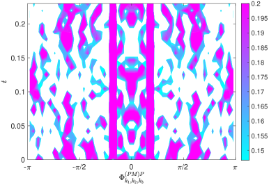
(c) ${\mathcal{P}}_{\mathcal{C}_{2}}^{(PM)P}(\Phi)(t)$

Figure 29: [Taylor-Green case, $k>2$:] Time evolution of the PDFs of the triad phase angle ${\mathcal{P}}_{\mathcal{C}_{2}}^{s_{1}s_{2}s_{3}}(\Phi)$ for triads of different types in the Navier-Stokes flow with the Taylor-Green initial condition. Only triad types with PDFs revealing variability of at least $\pm 5\%$ with respect to the uniform distribution equal to $1/2\pi\approx 0.16$ (corresponding to light blue colour in the plots), are shown: (a) “PMP”, (b) “P(PM)” and (c) “(PM)P ”. The PDFs for the triad types “PPP”, “PPM” and “PMM” are not shown, as they are essentially uniform (see table 5).

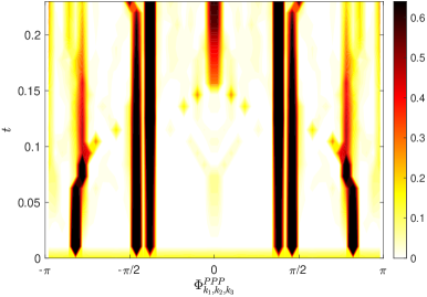
(a) ${\mathcal{W}}_{\mathcal{C}_{2}}^{PPP}(\Phi)(t)$

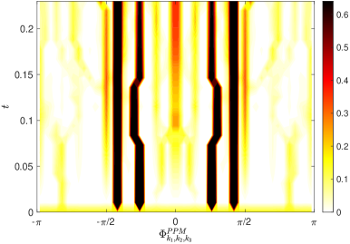
(b) ${\mathcal{W}}_{\mathcal{C}_{2}}^{PPM}(\Phi)(t)$

     

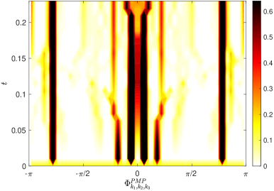
(c) ${\mathcal{W}}_{\mathcal{C}_{2}}^{PMP}(\Phi)(t)$

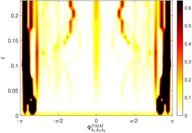
(d) ${\mathcal{W}}_{\mathcal{C}_{2}}^{PMM}(\Phi)(t)$

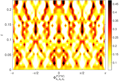
(e) ${\mathcal{W}}_{\mathcal{C}_{2}}^{P(PM)}(\Phi)(t)$

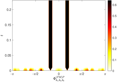
(f) ${\mathcal{W}}_{\mathcal{C}_{2}}^{(PM)P}(\Phi)(t)$

Figure 30: [Taylor-Green case, $k>2$:] Time evolution of the weighted PDF of the triad phase angle ${\mathcal{W}}_{\mathcal{C}_{2}}^{s_{1}s_{2}s_{3}}(\Phi)$, cf. expression (34), in the Navier-Stokes flow with the Taylor-Green initial condition for the triad types (a) “PPP”, (b) “PPM”, (c) “PMP” , (d) “PMM”, (e) “P(PM)” and (f) “(PM)P”. In these plots the uniform distribution corresponding to $1/2\pi\approx 0.16$ is depicted by yellow ($25\%$ of the colour bars).

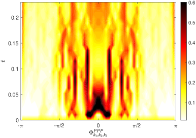
(a) ${\mathcal{W}}_{\mathcal{C}_{10}}^{PPP}(\Phi)(t)$

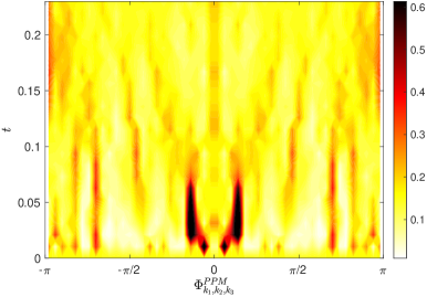
(b) ${\mathcal{W}}_{\mathcal{C}_{10}}^{PPM}(\Phi)(t)$

     

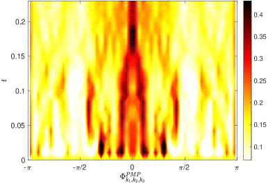
(c) ${\mathcal{W}}_{\mathcal{C}_{10}}^{PMP}(\Phi)(t)$

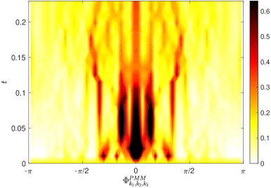
(d) ${\mathcal{W}}_{\mathcal{C}_{10}}^{PMM}(\Phi)(t)$

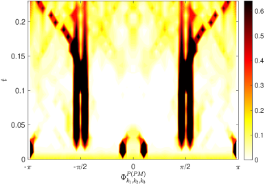
(e) ${\mathcal{W}}_{\mathcal{C}_{10}}^{P(PM)}(\Phi)(t)$

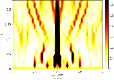
(f) ${\mathcal{W}}_{\mathcal{C}_{10}}^{(PM)P}(\Phi)(t)$

Figure 31: [Taylor-Green case, $k>10$:] Time evolution of the weighted PDF of the triad phase angle ${\mathcal{W}}_{\mathcal{C}_{10}}^{s_{1}s_{2}s_{3}}(\Phi)$, cf. expression (34), in the Navier-Stokes flow with the Taylor-Green initial condition for the triad types (a) “PPP”, (b) “PPM”, (c) “PMP” , (d) “PMM”, (e) “P(PM)” and (f) “(PM)P”. In these plots the uniform distribution corresponding to $1/2\pi\approx 0.16$ is depicted by yellow ($25\%$ of the colour bars).

5 Discussion and Conclusions

The goal of our study is to shed light on the nature of nonlinear modal interactions realizing the most extreme (in terms of amplification of the enstrophy) scenarios achievable in 1D Burgers and 3D Navier-Stokes flows. To provide context, we compare these interactions against the modal interactions occurring under generic and unimodal initial conditions in such flows. To address these questions we introduce analysis tools specifically designed to probe elementary triadic interactions responsible for the transfer of energy across scales and deploy these diagnostic tools to investigate Burgers and Navier-Stokes flows with different initial conditions given in table 1. The extreme initial conditions are constructed to maximize the finite-time growth of enstrophy, which serves as a measure of the regularity of the solution, by solving PDE-constrained optimization problems of the type (7) (Ayala & Protas, 2011; Kang et al., 2020). A remarkable feature of the 1D viscous Burgers and 3D Navier-Stokes flows obtained form such extreme initial conditions is that they are characterized by the same power-law dependence of the maximum attained enstrophy on the initial enstrophy ${\mathcal{E}}_{0}$ given by relation (8). The generic initial conditions are obtained from the extreme initial data by removing the spatial coherence while retaining its energy spectrum. The unimodal initial data has a small number of Fourier components and is taken in the form of the Taylor-Green vortex (Taylor & Green, 1937) in the case of the 3D Navier-Stokes flow.

The first main finding is that while under the extreme initial data 1D viscous Burgers flows and 3D Navier-Stokes flows reveal the same relative level of enstrophy amplification by nonlinear effects, this behaviour is realized by entirely different forms of modal interactions. More precisely, 1D Burgers flows, both inviscid and viscous, reveal highly coherent behaviour with triad phases displaying preferential alignment at two values, namely, $\pm\pi/2$, cf. figures 10(b) and 14(b). However, the flux-carrying triads have phase values predominantly aligned at $\pi/2$, cf. figures 10(b) and 14(b), which saturates the nonlinearity and therefore maximizes the energy flux towards small scales. On the other hand, in 3D Navier-Stokes flows with the extreme initial data the level of coherence is significantly lower: the various classes of helical triads exhibit phase distributions much closer to uniform, cf. table 3 and figure 21. Again, as in the 1D Burgers case, the flux-carrying triads in 3D Navier-Stokes flows do show a high level of coherence, but their phase values take a broader range of preferred values forming complicated time-dependent patterns, cf. figures 23 and 25. Thus, in 3D Navier-Stokes flows the energy flux to small scales is realized by a small only subset of helical triads. Interestingly, the solutions of both the 1D viscous Burgers system and the 3D Navier-Stokes system with the extreme initial data exhibit negative flux corresponding to the inverse energy cascade at early times (figures 12(b) and 19(b)). We refer to this as the “slingshot” effect which allows the flow to reorganize in order to reduce enstrophy production and conserve energy at early stages before a burst of flux is released towards small scales in anticipation of the instant of time when the enstrophy is to be maximized. The triadic interactions realizing this early-time negative flux have again quite different properties in the two cases, with the 1D Burgers flow exhibiting a significantly higher level of coherence.

The second main finding concerns the role of initial coherence. Comparison of the results for the 1D viscous Burgers flows and 3D Navier-Stokes flows corresponding to the extreme versus the generic initial conditions (i.e., the latter having the initial phases uniformly randomized), shows striking similarities between these two types of flows. The maximum attained enstrophy is reduced only slightly in the flows with the generic initial condition, cf. figures 7(b) and 16(b), which also reveal the “slingshot” effect, albeit weaker than the case with the extreme initial data. Contributions to the total flux from helical triads of different types are also remarkably similar in 3D Navier-Stokes flows with the extreme and generic initial conditions, cf. figures 22(b)(a–f), as are the corresponding time evolutions of the helical triad phases.

The third main finding, focusing now on the 3D Navier-Stokes flows, concerns the comparison between the flows with the extreme or generic initial condition on the one hand and the flow with the Taylor-Green initial condition on the other. As expected, when compared with the extreme or generic cases, the Taylor-Green flow shows a smaller level of flux in the inertial range (i.e., flux towards $k>2$), and an even smaller proportion of flux in the dissipative range (i.e., flux towards $k>10$). These differences are consistent with the fact that the flow with the extreme initial condition is designed to maximize the flux towards small scales: energy does not spend too long transitioning from the inertial range to the dissipative range so as not to be dissipated too early. In contrast, a salient feature of the Taylor-Green flow, observed at all spatial scales, is that the flux-carrying helical triads display a less dynamical, more rigid pattern of phase coherence, with very persistent narrow bands of preferred phase values, cf. figures 30 and 31. Moreover, in the inertial range, represented by the flux towards wavenumbers $k>2$, the Taylor-Green flow shows quite a different distribution of the main helical triad contributors to the direct cascade (i.e., the flux towards small scales), with the boundary triad type (PM)P being the most important contributor by far, cf. figures 22(b)(a,c,e). With reference to the same figures, in the Taylor-Green case the main contributor to the inverse cascade (i.e., the flux towards large scales) is the PMM helical triad type, and not the PPP type, which is the main contributor in the extreme and generic cases. In contrast, in the dissipative range, represented by the flux towards wavenumbers $k>10$, the behaviour of the Taylor-Green flow is qualitatively similar to the extreme and generic cases, and even quantitatively similar in terms of the relative contribution from the different helical triad types to the direct cascade, cf. figures 22(b)(b,d,f).

We provide a quick comparison of the results for the flows with the extreme and generic initial conditions against the paradigm suggested by Waleffe’s instability assumption and the classification of helical triads (Waleffe, 1992). First, we focus on the inertial range, where most of the flux occurs. In particular, regarding the flux towards the region with $k>2$, cf. figures 22(b)(a,c,e), its main contributor is the set of Class III helical triads, or PMP in our notation; this is quite in line with Waleffe’s paradigm, according to which the strength of the transfers towards small scales is the largest in that class (see the thick arrows in figure 3). The second main contributor is the new set of helical triads we introduced, the (PM)P triads, corresponding to the intersection $|\mathbf{k}_{1}|=|\mathbf{k}_{2}|$ between Class II and Class III helical triads. Again, referring to figure 3, this is quite in line with Waleffe’s paradigm.

The contribution by the PPP helical triads (Class I in Waleffe’s notation) to the flux is, fortunately, a feature that can be compared against all quantitative works on the subject (the other triad types are more difficult to compare due to differences in their definitions used by different research groups). It has been recently found in studies of forced statistically stationary turbulence (Sahoo & Biferale, 2018; Alexakis, 2017; Alexakis & Biferale, 2018) that the PPP helical triads contribute with an inverse-cascade flux at wavenumbers in the inertial range and with a direct-cascade flux in the dissipative range. Our results, being based on freely decaying turbulence from extreme or generic initial conditions, confirm this, even quantitatively, if one assumes (see, for example, Frisch (1995)) that the state of the maximum dissipation in a transient evolution is a proxy for a statistically stationary turbulence in a forced evolution, at least considering energy spectra and energy fluxes. Regarding the flux towards the region with $k>2$, which sits in the inertial range, we find that the PPP contribution is negative and of the order of 10% of the total flux in absolute terms near the time of the maximum dissipation, which is in quantitative agreement with the works cited above. Regarding the flux towards the region with $k>10$, which sits in the dissipative range, we find that the PPP contribution is positive and of the order of 30% of the total flux in absolute terms near the time of the maximum dissipation, again in quantitative agreement with the works cited above. It is worth mentioning that the case of the flow with the Taylor-Green initial condition leads to qualitatively different results in the inertial-range fluxes (namely, the fluxes towards the region with $k>2$): the PPP contribution to the inverse cascade is there but is small and the main contribution comes from the PMM helical triad type (Class II in Waleffe’s notation), cf. figures 22(b)(a,c,e).

It is well known that appearance of small scales and singularity formation in solutions of time-dependent PDE problems can be conveniently characterized in terms of the evolution of singularities in the complex extensions of these fields (Weideman, 2003; Matsumoto et al., 2008; Siegel & Caflisch, 2009). In particular, blow-up of the solution is signaled by the collapse of some of these complex-plane singularities onto the real axis (i.e., when the width of the analyticity strip shrinks to zero). As regards the diagnostics employed in the present study, it is an interesting open question how properties of triad phases in a flow can be deduced from the evolution of complex-plane singularities characterizing these solutions, and vice versa.

Appendix A Minimizing the Blow-up Time in the 1D Inviscid Burgers Equation

In this appendix we demonstrate that the problem of finding an initial condition $u_{0}\in H^{1}(\Omega)$ for the inviscid Burgers system (4) with a fixed enstrophy ${\mathcal{E}}_{0}>0$ such that the corresponding solution blows up in the shortest time $t^{*}(u_{0})$ does not in fact admit a solution. In other words, it is possible to find initial data $u_{0}$ with ${\mathcal{E}}(u_{0})={\mathcal{E}}_{0}$ such that the corresponding solution of (4) blows up arbitrarily quickly. We thus have

Theorem 1

The minimization problem

$$\min_{u_{0}\in H^{1}(\Omega)}t^{*}(u_{0})\quad\text{subject to}\quad{\mathcal{E}}(u_{0})={\mathcal{E}}_{0}$$ (37)

has no solution.

Proof 1

Since for the inviscid Burgers equation (4) we have an explicit expression for the blow-up time $t^{*}=-1/\left[\inf_{x\in\Omega}{\partial u_{0}\over\partial x}(x)\right]$, problem (37) is equivalent to

$$\max_{g\in L^{2}(\Omega)}\|g\|_{L^{\infty}}\quad\text{subject to}\quad\frac{1}{2}\|g\|_{L^{2}}^{2}={\mathcal{E}}_{0},$$ (38)

where $g:={\partial u_{0}\over\partial x}$. It is easy to construct a sequence of functions $g_{n}$ with a fixed $L^{2}$ norm and vanishing support $\lim_{n\rightarrow\infty}|\operatorname{supp}_{x\in\Omega}g_{n}(x)|=0$ such that their $L^{\infty}$ norms increase without bound, $\lim_{n\rightarrow\infty}\|g_{n}\|_{L^{\infty}}=\infty$, thus demonstrating that a maximum is not attained in problem (38).

Appendix B Proof of the Symmetry of Conjugate Triads under Zero Helicity Assumption

In this appendix we state and prove the following theorem implying the symmetry of conjugate triads.

Theorem 2

If the incompressible velocity field ${\mathbf{u}}$ satisfies the condition of oddity under the parity transformation, namely,

$$\mathbf{u}(-\mathbf{x},t)=-\mathbf{u}(\mathbf{x},t)\qquad\text{for all}\qquad\mathbf{x}\in\mathbb{R}^{3},\quad t\in\mathbb{R},$$ (39)

then:

1. the helical modes $u_{\mathbf{k}}^{+},u_{\mathbf{k}}^{-}$ satisfy the identity

   $$u_{-\mathbf{k}}^{s}=-u_{\mathbf{k}}^{-s},\qquad\text{for all}\qquad\mathbf{k}\in\mathbb{Z}^{3}\setminus\{\mathbf{0}\},\quad s=\pm,$$

2. the helicity spectrum is zero: ${\mathcal{H}}_{{\mathbf{k}}}=0,\quad\text{for all}\quad{\mathbf{k}}\in\mathbb{Z}^{3}\setminus\{\mathbf{0}\}$, cf. (22b), and

3. the generalized helical triad phases (27) exhibit the following invariance with respect to the transformations $s_{j}\rightarrow-s_{j}$, $j=1,2,3$:

   $$\Phi_{{\mathbf{k}_{1}}{\mathbf{k}_{2}}{\mathbf{k}_{3}}}^{-s_{1}\,-s_{2}\,-s_{3}}=-\Phi_{{\mathbf{k}_{1}}{\mathbf{k}_{2}}{\mathbf{k}_{3}}}^{s_{1}\,\,s_{2}\,\,s_{3}},\qquad\text{whenever}\qquad{\mathbf{k}}_{1}+{\mathbf{k}}_{2}+{\mathbf{k}}_{3}={\mathbf{0}}.$$ (40)

Proof 2

Assuming condition (39) is satisfied, let us first establish the corresponding relation for the Fourier components of the velocity field. From equation (18) we have

$$\mathbf{u}(\mathbf{x},t)=\sum_{\mathbf{k}\in\mathbb{Z}^{3}\setminus\mathbf{0}}\mathbf{\widehat{u}}_{\mathbf{k}}(t)\exp(2\pi i\mathbf{k}\cdot\mathbf{x})\,,$$

so

$$\mathbf{u}(-\mathbf{x},t)=\sum_{\mathbf{k}\in\mathbb{Z}^{3}\setminus\mathbf{0}}\mathbf{\widehat{u}}_{\mathbf{k}}(t)\exp(-2\pi i\mathbf{k}\cdot\mathbf{x})=\sum_{\mathbf{k}\in\mathbb{Z}^{3}\setminus\mathbf{0}}\mathbf{\widehat{u}}_{-\mathbf{k}}(t)\exp(2\pi i\mathbf{k}\cdot\mathbf{x})\,,$$

where in the last equality we relabelled the wavevectors from $\mathbf{k}$ to $-\mathbf{k}$. Equating this expression with the Fourier expansion of $-\mathbf{u}(\mathbf{x},t)$ we obtain, from uniqueness of the expansion,

$$\mathbf{\widehat{u}}_{-\mathbf{k}}(t)=-\mathbf{\widehat{u}}_{\mathbf{k}}(t),\qquad\text{for \,\, all}\qquad\mathbf{k}\in\mathbb{Z}^{3}\setminus\{\mathbf{0}\}\,.$$ (41)

Now we prove each of the claims in the theorem:

1. The helical mode decomposition (19) gives

   $$\mathbf{\widehat{u}}_{\mathbf{k}}(t)=\mathbf{h}_{\mathbf{k}}^{+}u_{\mathbf{k}}^{+}(t)+\mathbf{h}_{\mathbf{k}}^{-}u_{\mathbf{k}}^{-}(t)\,$$

   and noting that $\mathbf{h}_{-\mathbf{k}}^{s}=\mathbf{h}_{\mathbf{k}}^{-s}$ we obtain

   $$\mathbf{\widehat{u}}_{-\mathbf{k}}(t)=\mathbf{h}_{-\mathbf{k}}^{+}u_{-\mathbf{k}}^{+}(t)+\mathbf{h}_{-\mathbf{k}}^{-}u_{-\mathbf{k}}^{-}(t)=\mathbf{h}_{\mathbf{k}}^{-}u_{-\mathbf{k}}^{+}(t)+\mathbf{h}_{\mathbf{k}}^{+}u_{-\mathbf{k}}^{-}(t).$$

   Invoking uniqueness of the helical decomposition, relation (41) is equivalent to

   $$u_{-\mathbf{k}}^{-}(t)=-u_{\mathbf{k}}^{+}(t)\,,\qquad\mathbf{k}\in\mathbb{Z}^{3}\setminus\{\mathbf{0}\}\,.$$

   This of course also implies that $u_{-\mathbf{k}}^{+}(t)=-u_{\mathbf{k}}^{-}(t)$.

2. The helicity spectrum is defined as

   $$\mathcal{H}_{\mathbf{k}}(t)=|u_{\mathbf{k}}^{+}(t)|^{2}-|u_{\mathbf{k}}^{-}(t)|^{2}\,.$$

   Since the original velocity field is real-valued, we obtain $u_{-\mathbf{k}}^{s}(t)=[u_{\mathbf{k}}^{s}(t)]^{*}$, such that

   $$|u_{\mathbf{k}}^{-}(t)|=|u_{\mathbf{-k}}^{-}(t)|=|{-u_{\mathbf{k}}^{+}(t)}|=|u_{\mathbf{k}}^{+}(t)|,$$

   implies $\mathcal{H}_{\mathbf{k}}(t)=0\,,\quad\mathbf{k}\in\mathbb{Z}^{3}\setminus\{\mathbf{0}\}$.

3. The generalized helical triad phases are obtained, mod $2\pi$, from combining equations (27) and (28):

   $$\Phi_{{\mathbf{k}_{1}}{\mathbf{k}_{2}}{\mathbf{k}_{3}}}^{s_{1}\,\,s_{2}\,\,s_{3}}=\phi_{\mathbf{k}_{1}}^{s_{1}}+\phi_{\mathbf{k}_{2}}^{s_{2}}+\phi_{\mathbf{k}_{3}}^{s_{3}}+\arg[\mathbf{h}_{\mathbf{k}_{1}}^{s_{1}}\times\mathbf{h}_{\mathbf{k}_{2}}^{s_{2}}\cdot\mathbf{h}_{\mathbf{k}_{3}}^{s_{3}}]+\begin{cases}\arg(s_{2}k_{2}-s_{1}k_{1}),&\text{if}\quad\mathbf{k}_{3}\in\mathcal{C};\mathbf{k}_{1},\mathbf{k}_{2}\in\mathcal{U}\setminus\mathcal{C}\\ \arg(s_{2}k_{2}-s_{3}k_{3}),&\text{if}\quad\mathbf{k}_{3},\mathbf{k}_{2}\in\mathcal{C};\mathbf{k}_{1}\in\mathcal{U}\setminus\mathcal{C}\end{cases}\,,$$

   where $\phi_{\mathbf{k}}^{s}=\arg u_{\mathbf{k}}^{s}(t)$. We now analyze the behaviour of this expression under the transformation $s_{j}\to-s_{j},\,\,j=1,2,3$. First, using part 1 of the theorem, we get:

   $$\phi_{\mathbf{k}}^{-s}=\arg u_{\mathbf{k}}^{-s}(t)=\arg(-u_{-\mathbf{k}}^{s}(t))=\pi+\phi_{-\mathbf{k}}^{s}=\pi-\phi_{\mathbf{k}}^{s}\,,$$

   where the last equality follows from the reality condition. Second, from the definition of the helical basis vectors we have

   $$\mathbf{h}_{\mathbf{k}}^{-s}=[\mathbf{h}_{\mathbf{k}}^{s}]^{*}\,.$$

   Third, we have, mod $2\pi$, $\arg(-s_{2}k_{2}-(-s_{1})k_{1})=\pi-\arg(s_{2}k_{2}-s_{1}k_{1})$, and so on. Therefore, we obtain

   $$\Phi_{{\mathbf{k}_{1}}{\mathbf{k}_{2}}{\mathbf{k}_{3}}}^{-s_{1}\,\,-s_{2}\,\,-s_{3}}=\phi_{\mathbf{k}_{1}}^{-s_{1}}+\phi_{\mathbf{k}_{2}}^{-s_{2}}+\phi_{\mathbf{k}_{3}}^{-s_{3}}+\arg[\mathbf{h}_{\mathbf{k}_{1}}^{-s_{1}}\times\mathbf{h}_{\mathbf{k}_{2}}^{-s_{2}}\cdot\mathbf{h}_{\mathbf{k}_{3}}^{-s_{3}}]+\begin{cases}\arg(-s_{2}k_{2}+s_{1}k_{1}),&\text{if}\quad\mathbf{k}_{3}\in\mathcal{C};\mathbf{k}_{1},\mathbf{k}_{2}\in\mathcal{U}\setminus\mathcal{C}\,,\\ \arg(-s_{2}k_{2}+s_{3}k_{3}),&\text{if}\quad\mathbf{k}_{3},\mathbf{k}_{2}\in\mathcal{C};\mathbf{k}_{1}\in\mathcal{U}\setminus\mathcal{C}\,,\end{cases}$$

   $$=3\pi-\left(\phi_{\mathbf{k}_{1}}^{s_{1}}+\phi_{\mathbf{k}_{2}}^{s_{2}}+\phi_{\mathbf{k}_{3}}^{s_{3}}\right)+\arg[\mathbf{h}_{\mathbf{k}_{1}}^{s_{1}}\times\mathbf{h}_{\mathbf{k}_{2}}^{s_{2}}\cdot\mathbf{h}_{\mathbf{k}_{3}}^{s_{3}}]^{*}+\pi-\begin{cases}\arg(s_{2}k_{2}-s_{1}k_{1}),&\text{if}\quad\mathbf{k}_{3}\in\mathcal{C};\mathbf{k}_{1},\mathbf{k}_{2}\in\mathcal{U}\setminus\mathcal{C}\,,\\ \arg(s_{2}k_{2}-s_{3}k_{3}),&\text{if}\quad\mathbf{k}_{3},\mathbf{k}_{2}\in\mathcal{C};\mathbf{k}_{1}\in\mathcal{U}\setminus\mathcal{C}\,,\end{cases}$$

   $$=4\pi-\left(\phi_{\mathbf{k}_{1}}^{s_{1}}+\phi_{\mathbf{k}_{2}}^{s_{2}}+\phi_{\mathbf{k}_{3}}^{s_{3}}\right)-\arg[\mathbf{h}_{\mathbf{k}_{1}}^{s_{1}}\times\mathbf{h}_{\mathbf{k}_{2}}^{s_{2}}\cdot\mathbf{h}_{\mathbf{k}_{3}}^{s_{3}}]-\begin{cases}\arg(s_{2}k_{2}-s_{1}k_{1}),&\text{if}\quad\mathbf{k}_{3}\in\mathcal{C};\mathbf{k}_{1},\mathbf{k}_{2}\in\mathcal{U}\setminus\mathcal{C}\,,\\ \arg(s_{2}k_{2}-s_{3}k_{3}),&\text{if}\quad\mathbf{k}_{3},\mathbf{k}_{2}\in\mathcal{C};\mathbf{k}_{1}\in\mathcal{U}\setminus\mathcal{C}\,,\end{cases}$$

   so that, mod $2\pi$, we finally arrive at

   $$\Phi_{{\mathbf{k}_{1}}{\mathbf{k}_{2}}{\mathbf{k}_{3}}}^{-s_{1}\,\,-s_{2}\,\,-s_{3}}=-\Phi_{{\mathbf{k}_{1}}{\mathbf{k}_{2}}{\mathbf{k}_{3}}}^{s_{1}\,\,s_{2}\,\,s_{3}}\,.$$

Appendix C Fourier-Lagrange Formula for the Inviscid Burgers Equation

In order to determine the solutions of the inviscid Burgers system (4) with initial conditions (9) and (11), we will use an adaptation of the Fourier-Lagrange formula originally proposed by Fournier & Frisch (1983) which provides an exact expression for the Fourier coefficients $\widehat{u}_{k}(t)$ of the solution for $0\leq t<t^{*}$. One difference with respect to the approach in Fournier & Frisch (1983) is that here we work on a periodic, rather than unbounded, spatial domain. As a starting point, we write the solution of system (4) in terms of the flowmap $\xi=\xi(a,t)$, where $a\in[0,1]$ is the Lagrangian coordinate, as Kreiss & Lorenz (2004)

$$u(\xi(a,t),t)=u_{0}(a),\quad\xi(a,t)=a+tu_{0}(a),\quad a\in[0,1],\quad 0\leq t<t^{*}.$$ (42)

Then, the Fourier coefficients of the solution can be expressed as, cf. (12),

$$\widehat{u}_{k}(t) =\int_{0}^{1}e^{-2\pi ikx}u(x,t)\,dx=\int_{0}^{1}e^{-2\pi ik\xi(a,t)}u(\xi(a,t),t)\,d\xi$$

$$=\int_{0}^{1}\frac{d}{d\xi}\left(\frac{-1}{2\pi ik}e^{-2\pi ik\xi(a,t)}\right)u(\xi(a,t),t)\,d\xi=\frac{1}{2\pi ik}\int_{0}^{1}e^{-2\pi ik\xi(a,t)}\frac{du}{d\xi}(\xi(a,t),t)\,d\xi$$

$$=\frac{1}{2\pi ik}\int_{0}^{1}e^{-2\pi ik\left[a+tu_{0}(a)\right]}\frac{du_{0}}{da}(a)\,da,$$

where we used (42), performed integration by parts with respect to $\xi$ and employed the identity $\frac{du}{da}(\xi(a,t),t)=\frac{du_{0}}{da}(a)$ which follows from (42) together with the chain rule. Next, defining $\eta(a,t):=\xi(a,t)-a=tu_{0}(a)$, we have

$$\widehat{u}_{k}(t) =\frac{1}{2\pi ikt}\int_{0}^{1}{\partial\eta\over\partial a}(a,t)e^{-2\pi ik\left[a+\eta(a,t)\right]}\,da$$

$$=\frac{1}{2\pi ikt}\int_{0}^{1}\left(\frac{-1}{2\pi ik}\right){\partial\over\partial a}\left[e^{-2\pi ik\eta(a,t)}\right]e^{-2\pi ika}\,da$$

$$=\frac{-1}{2\pi ikt}\int_{0}^{1}e^{-2\pi ik\left[a+tu_{0}(a)\right]}\,da,\quad k\neq 0,\quad 0<t<t^{*},$$ (43)

where we again performed integration by parts, this time with respect to $a$.

For a given initial condition $u_{0}$, relation (43) allows for a straightforward evaluation of the Fourier coefficients of the solution of (4) by performing an integral. For example, using the unimodal initial condition (9), we obtain

$$\widehat{u}_{k}(t) =\frac{-1}{2\pi ikt}\int_{0}^{1}e^{-2\pi ik\left[a+tA\sin(2\pi a)\right]}\,da,$$

$$=\frac{-1}{2\pi ikt}J_{k}(-kAt),\quad k\neq 0,\quad 0<t<t^{*},$$ (44)

where we have used the integral representation of the Bessel functions of the first kind $J_{k}(x)=\frac{1}{2\pi}\int_{-\pi}^{\pi}e^{i[x\sin(\tau)-n\tau]}\,d\tau$ (DLMF, 2020). An expression for the Fourier coefficients of the solution corresponding to the extreme initial condition (11) can be obtained in a similar manner.

References

- Adams & Fournier (2005) Adams, R. A. & Fournier, J. F. 2005 Sobolev Spaces. Elsevier.
- Alexakis (2017) Alexakis, Alexandros 2017 Helically decomposed turbulence. Journal of Fluid Mechanics 812, 752–770.
- Alexakis & Biferale (2018) Alexakis, Alexandros & Biferale, Luca 2018 Cascades and transitions in turbulent flows. Physics Reports 767, 1–101.
- Ayala & Protas (2011) Ayala, D. & Protas, B. 2011 On maximum enstrophy growth in a hydrodynamic system. Physica D 240, 1553–1563.
- Ayala & Protas (2017) Ayala, D. & Protas, B. 2017 Extreme vortex states and the growth of enstrophy in 3D incompressible flows. Journal of Fluid Mechanics 818, 772–806.
- Bec & Khanin (2007) Bec, Jérémie & Khanin, Konstantin 2007 Burgers turbulence. Physics Reports 447 (1–2), 1–66.
- Biferale et al. (2012) Biferale, Luca, Musacchio, Stefano & Toschi, Federico 2012 Inverse energy cascade in three-dimensional isotropic turbulence. Phys. Rev. Lett. 108, 164501.
- Biferale et al. (2013) Biferale, L, Musacchio, Stefano & Toschi, F 2013 Split energy-helicity cascades in three-dimensional homogeneous and isotropic turbulence. Journal of Fluid Mechanics 730, 309 327.
- Brachet (1991) Brachet, M. E. 1991 Direct simulation of three-dimensional turbulence in the Taylor-Green vortex. Fluid Dynamics Research 8, 1–8.
- Brachet et al. (1983) Brachet, M. E., Meiron, D. I., Orszag, S. A., Nickel, B. G., Morf, R. H. & Frisch, U. 1983 Small-scale structure of the Taylor-Green vortex. Journal of Fluid Mechanics 130, 411–452.
- Bustamante & Brachet (2012) Bustamante, M. D. & Brachet, M. 2012 Interplay between the Beale-Kato-Majda theorem and the analyticity-strip method to investigate numerically the incompressible Euler singularity problem. Phys. Rev. E 86, 066302.
- Buzzicotti et al. (2016) Buzzicotti, Michele, Murray, Brendan P., Biferale, Luca & Bustamante, Miguel D. 2016 Phase and precession evolution in the burgers equation. The European Physical Journal E 39 (3), 34.
- Chen et al. (2003) Chen, Qiaoning, Chen, Shiyi & Eyink, Gregory L 2003 The joint cascade of energy and helicity in three-dimensional turbulence. Physics of Fluids 15 (2), 361–374.
- Constantin & Majda (1988) Constantin, Peter & Majda, Andrew 1988 The beltrami spectrum for incompressible fluid flows. Communications in mathematical physics 115 (3), 435–456.
- Craya (1957) Craya, Antoine 1957 Contribution à l’analyse de la turbulence associée à des vitesses moyennes. PhD thesis, Université de Grenoble.
- De Pietro et al. (2015) De Pietro, Massimo, Biferale, Luca & Mailybaev, Alexei A 2015 Inverse energy cascade in nonlocal helical shell models of turbulence. Physical Review E 92 (4), 043021.
- DLMF (2020) DLMF 2020 NIST Digital Library of Mathematical Functions. http://dlmf.nist.gov/, Release 1.1.0 of 2020-12-15, f. W. J. Olver, A. B. Olde Daalhuis, D. W. Lozier, B. I. Schneider, R. F. Boisvert, C. W. Clark, B. R. Miller, B. V. Saunders, H. S. Cohl, and M. A. McClain, eds.
- Doering (2009) Doering, C. R. 2009 The 3D Navier-Stokes problem. Annual Review of Fluid Mechanics 41, 109–128.
- Fefferman (2000) Fefferman, C. L. 2000 Existence and smoothness of the Navier-Stokes equation. available at http://www.claymath.org/sites/default/files/navierstokes.pdf, Clay Millennium Prize Problem Description.
- Foias & Temam (1989) Foias, C. & Temam, R. 1989 Gevrey class regularity for the solutions of the Navier–Stokes equations. Journal of Functional Analysis 87, 359–369.
- Fournier & Frisch (1983) Fournier, J.-D. & Frisch, U. 1983 L’équation de Burgers déterministe et statistique (The deterministic and statistical Burgers equation). J. Méc. Théor. Appl. 2, 699–750.
- Frisch (1995) Frisch, Uriel 1995 Turbulence: The Legacy of AN Kolmogorov. Cambridge University Press.
- Herring (1974) Herring, JR 1974 Approach of axisymmetric turbulence to isotropy. The Physics of Fluids 17 (5), 859–872.
- Kang et al. (2020) Kang, Di, Yun, Dongfang & Protas, Bartosz 2020 Maximum amplification of enstrophy in three-dimensional Navier-Stokes flows. Journal of Fluid Mechanics 893, A22.
- Kraichnan (1959) Kraichnan, Robert H. 1959 The structure of isotropic turbulence at very high reynolds numbers. Journal of Fluid Mechanics 5 (4), 497?543.
- Kreiss & Lorenz (2004) Kreiss, H. & Lorenz, J. 2004 Initial-Boundary Value Problems and the Navier-Stokes Equations, Classics in Applied Mathematics, vol. 47. SIAM.
- Lesieur (1972) Lesieur, M 1972 Décomposition d’un champ de vitesse non divergent en ondes d’hélicité. Revue ‘Turbulence’. Observatoire de Nice .
- Matsumoto et al. (2008) Matsumoto, T., Bec, J. & Frisch, U. 2008 Complex-space singularities of 2D Euler flow in lagrangian coordinates. Physica D 237, 1951–1955.
- Moffatt (1969) Moffatt, H. K. 1969 The degree of knottedness of tangled vortex lines. Journal of Fluid Mechanics 35 (1), 117–129.
- Moffatt (2014) Moffatt, H. K. 2014 Note on the triad interactions of homogeneous turbulence. Journal of Fluid Mechanics 741, R3.
- Murray (2017) Murray, Brendan P. 2017 Fourier phase dynamics in turbulent non-linear systems. PhD Thesis, University College Dublin. Available at https://researchrepository.ucd.ie/handle/10197/10622.
- Murray & Bustamante (2018) Murray, Brendan P. & Bustamante, Miguel D. 2018 Energy flux enhancement, intermittency and turbulence via fourier triad phase dynamics in the 1-d burgers equation. Journal of Fluid Mechanics 850, 624–645.
- Protas et al. (2004) Protas, B., Bewley, T. & Hagen, G. 2004 A Comprehensive Framework for the Regularization of Adjoint Analysis in Multiscale PDE Systems. J. Comp. Phys. 195, 49–89.
- Rathmann & Ditlevsen (2016) Rathmann, Nicholas M & Ditlevsen, Peter D 2016 Role of helicity in triad interactions in three-dimensional turbulence investigated by a new shell model. Physical Review E 94 (3), 033115.
- Rathmann & Ditlevsen (2017) Rathmann, Nicholas M. & Ditlevsen, Peter D. 2017 Pseudo-invariants contributing to inverse energy cascades in three-dimensional turbulence. Phys. Rev. Fluids 2, 054607.
- Robinson (2020) Robinson, James C 2020 The Navier-Stokes regularity problem. Phil. Trans. R. Soc. A 378, 20190526.
- Sahoo & Biferale (2015) Sahoo, Ganapati & Biferale, Luca 2015 Disentangling the triadic interactions in navier-stokes equations. The European Physical Journal E 38 (10), 1–8.
- Sahoo & Biferale (2018) Sahoo, Ganapati & Biferale, Luca 2018 Energy cascade and intermittency in helically decomposed navier–stokes equations. Fluid Dynamics Research 50 (1), 011420.
- Siegel & Caflisch (2009) Siegel, M. & Caflisch, R. E. 2009 Calculation of complex singular solutions to the 3D incompressible Euler equations. Physica D 238, 2368–2379.
- Taylor & Green (1937) Taylor, G. I. & Green, A. E. 1937 Mechanism of the production of small eddies from large ones. Proceedings of the Royal Society of London A 158, 499–521.
- Waleffe (1992) Waleffe, Fabian 1992 The nature of triad interactions in homogeneous turbulence. Physics of Fluids A: Fluid Dynamics 4 (2), 350–363.
- Weideman (2003) Weideman, J. A. C. 2003 Computing the dynamics of complex singularities of nonlinear pdes. SIAM Journal on Applied Dynamical Systems 2 (2), 171–186.