Generative Adversarial Neural Architecture Search

Abstract

Despite the empirical success of neural architecture search (NAS) in deep learning applications, the optimality, reproducibility and cost of NAS schemes remain hard to assess. In this paper, we propose Generative Adversarial NAS (GA-NAS) with theoretically provable convergence guarantees, promoting stability and reproducibility in neural architecture search. Inspired by importance sampling, GA-NAS iteratively fits a generator to previously discovered top architectures, thus increasingly focusing on important parts of a large search space. Furthermore, we propose an efficient adversarial learning approach, where the generator is trained by reinforcement learning based on rewards provided by a discriminator, thus being able to explore the search space without evaluating a large number of architectures. Extensive experiments show that GA-NAS beats the best published results under several cases on three public NAS benchmarks. In the meantime, GA-NAS can handle ad-hoc search constraints and search spaces. We show that GA-NAS can be used to improve already optimized baselines found by other NAS methods, including EfficientNet and ProxylessNAS, in terms of ImageNet accuracy or the number of parameters, in their original search space.

1 Introduction

Neural architecture search (NAS) improves neural network model design by replacing the manual trial-and-error process with an automatic search procedure, and has achieved state-of-the-art performance on many computer vision tasks Elsken et al. (2018). Since the underlying search space of architectures grows exponentially as a function of the architecture size, searching for an optimum neural architecture is like looking for a needle in a haystack. A variety of search algorithms have been proposed for NAS, including random search (RS) Li and Talwalkar (2020), differentiable architecture search (DARTS) Liu et al. (2018), Bayesian optimization (BO) Kandasamy et al. (2018), evolutionary algorithm (EA) Dai et al. (2020), and reinforcement learning (RL) Pham et al. (2018).

Despite a proliferation of NAS methods proposed, their sensitivity to random seeds and reproducibility issues concern the community Li and Talwalkar (2020), Yu et al. (2019), Yang et al. (2019). Comparisons between different search algorithms, such as EA, BO, and RL, etc., are particularly hard, as there is no shared search space or experimental protocol followed by all these NAS approaches. To promote fair comparisons among methods, multiple NAS benchmarks have recently emerged, including NAS-Bench-101 Ying et al. (2019), NAS-Bench-201 Dong and Yang (2020), and NAS-Bench-301 Siems et al. (2020), which contain collections of architectures with their associated performance. This has provided an opportunity for researchers to fairly benchmark search algorithms (regardless of the search space in which they are performed) by evaluating how many queries to architectures an algorithm needs to make in order to discover a top-ranked architecture in the benchmark set Luo et al. (2020); Siems et al. (2020). The number of queries converts to an indicator of how many architectures need be evaluated in reality, which often forms the bottleneck of NAS.

In this paper, we propose Generative Adversarial NAS (GA-NAS), a provably converging and efficient search algorithm to be used in NAS based on adversarial learning. Our method is first inspired by the Cross Entropy (CE) method Rubinstein and Kroese (2013) in importance sampling, which iteratively retrains an architecture generator to fit to the distribution of winning architectures generated in previous iterations so that the generator will increasingly sample from more important regions in an extremely large search space. However, such a generator cannot be efficiently trained through back-propagation, as performance measurements can only be obtained for discretized architectures and thus the model is not differentiable. To overcome this issue, GA-NAS uses RL to train an architecture generator network based on RNN and GNN. Yet unlike other RL-based NAS schemes, GA-NAS does not obtain rewards by evaluating generated architectures, which is a costly procedure if a large number of architectures are to be explored. Rather, it learns a discriminator to distinguish the winning architectures from randomly generated ones in each iteration. This enables the generator to be efficiently trained based on the rewards provided by the discriminator, without many true evaluations. We further establish the convergence of GA-NAS in a finite number of steps, by connecting GA-NAS to an importance sampling method with a symmetric Jensen–Shannon (JS) divergence loss.

Extensive experiments have been performed to evaluate GA-NAS in terms of its convergence speed, reproducibility and stability in the presence of random seeds, scalability, flexibility of handling constrained search, and its ability to improve already optimized baselines. We show that GA-NAS outperforms a wide range of existing NAS algorithms, including EA, RL, BO, DARTS, etc., and state-of-the-art results reported on three representative NAS benchmark sets, including NAS-Bench-101, NAS-Bench-201, and NAS-Bench-301—it consistently finds top ranked architectures within a lower number of queries to architecture performance. We also demonstrate the flexibility of GA-NAS by showing its ability to incorporate ad-hoc hard constraints and its ability to further improve existing strong architectures found by other NAS methods. Through experiments on ImageNet, we show that GA-NAS can enhance EfficientNet-B0 Tan and Le (2019) and ProxylessNAS Cai et al. (2018) in their respective search spaces, resulting in architectures with higher accuracy and/or smaller model sizes.

2 Related Work

A typical NAS method includes a search phase and an evaluation phase. This paper is concerned with the search phase, of which the most important performance criteria are robustness, reproducibility and search cost. DARTS Liu et al. (2018) has given rise to numerous optimization schemes for NAS Xie et al. (2018). While the objectives of these algorithms may vary, they all operate in the same or similar search space. However, Yu et al. (2019) demonstrates that DARTS performs similarly to a random search and its results heavily dependent on the initial seed. In contrast, GA-NAS has a convergence guarantee under certain assumptions and its results are reproducible.

NAS-Bench-301 Siems et al. (2020) provides a formal benchmark for all $10^{18}$ architectures in the DARTS search space. Preceding NAS-Bench-301 are NAS-Bench-101 Ying et al. (2019) and NAS-Bench-201 Dong and Yang (2020). Besides the cell-based searches, GA-NAS also applies to macro-search Cai et al. (2018); Tan et al. (2019), which searches for an ordering of a predefined set of blocks.

On the other hand, several RL-based NAS methods have been proposed. ENAS Pham et al. (2018) is the first Reinforcement Learning scheme in weight-sharing NAS. TuNAS Bender et al. (2020) shows that guided policies decisively exceed the performance of random search on vast search spaces. In comparison, GA-NAS proves to be a highly efficient RL solution to NAS, since the rewards used to train the actor come from the discriminator instead of from costly evaluations.

Hardware-friendly NAS algorithms take constraints such as model size, FLOPS, and inference time into account Cai et al. (2018); Tan et al. (2019), usually by introducing regularizers into the loss functions. Contrary to these methods, GA-NAS can support ad-hoc search tasks, by enforcing customized hard constraints in importance sampling instead of resorting to approximate penalty terms.

3 The Proposed Method

In this section, we present Generative Adversarial NAS (GA-NAS) as a search algorithm to discover top architectures in an extremely large search space. GA-NAS is theoretically inspired by the importance sampling approach and implemented by a generative adversarial learning framework to promote efficiency.

We can view a NAS problem as a combinatorial optimization problem. For example, suppose that $x$ is a Directed Acyclic Graph (DAG) connecting a certain number of operations, each chosen from a predefined operation set. Let $S(x)$ be a real-valued function representing the performance, e.g., accuracy, of $x$. In NAS, we optimize $S(x)$ subject to $x\in\mathcal{X}$, where $\mathcal{X}$ denotes the underlying search space of neural architectures.

One approach to solving a combinatorial optimization problem, especially the NP-hard ones, is to view the problem in the framework of importance sampling and rare event simulation Rubinstein and Kroese (2013). In this approach we consider a family of probability densities $\{p(.;\theta)\}_{\theta\in\Theta}$ on the set $\mathcal{X}$, with the goal of finding a density $p(.;\theta^{*})$ that assigns higher probabilities to optimal solutions to the problem. Then, with high probability, the sampled solution from the density $p(.;\theta^{*})$ will be an optimal solution. This approach for importance sampling is called the Cross-Entropy method.

3.1 Generative Adversarial NAS

Algorithm 1 GA-NAS Algorithm

1:Input: An initial set of architectures $\mathcal{X}_{0}$; Discriminator $D$; Generator $G(x;\theta_{0})$; A positive integer $k$;

2:for $t=1,2,\ldots,T$ do

3:     $\mathcal{T}\leftarrow$ top $k$ architectures of $\bigcup_{i=0}^{t-1}\mathcal{X}_{i}$ according to the performance evaluator $S(.)$.

4:     Train $G$ and $D$ to obtain their parameters

$$\begin{multlined}(\theta_{t},\phi_{t})\longleftarrow\arg\min_{\theta_{t}}\max_{\phi_{t}}V\left(G_{\theta_{t}},D_{\phi_{t}}\right)=\\ \mathbb{E}_{x\sim p_{\mathcal{T}}}\left[\log D_{\phi_{t}}(x)\right]+\mathbb{E}_{x\sim p(x;\theta_{t})}\left[\log\left(1-D_{\phi_{t}}(x)\right)\right].\end{multlined}(\theta_{t},\phi_{t})\longleftarrow\arg\min_{\theta_{t}}\max_{\phi_{t}}V\left(G_{\theta_{t}},D_{\phi_{t}}\right)=\\ \mathbb{E}_{x\sim p_{\mathcal{T}}}\left[\log D_{\phi_{t}}(x)\right]+\mathbb{E}_{x\sim p(x;\theta_{t})}\left[\log\left(1-D_{\phi_{t}}(x)\right)\right].$$

5:     Let $G(x;\theta_{t})$ generate a new set of architectures $\mathcal{X}_{t}$.

6:     Evaluate the performance $S(x)$ of every $x\in\mathcal{X}_{t}$.

7:end for

GA-NAS is presented in Algorithm 1, where a discriminator $D$ and a generator $G$ are learned over iterations. In each iteration of GA-NAS, the generator $G$ will generate a new set of architectures $\mathcal{X}_{t}$, which gets combined with previously generated architectures. A set of top performing architectures $\mathcal{T}$, which we also call true set of architectures, is updated by selecting top $k$ from already generated architectures and gets improved over time.

Following the GAN framework, originally proposed by Goodfellow et al. (2014), the discriminator $D$ and the generator $G$ are trained by playing a two-player minimax game whose corresponding parameters $\phi_{t}$ and $\theta_{t}$ are optimized by Step 4 of Algorithm 1. After Step 4, $G$ learns to generate architectures to fit to the distribution of $\mathcal{T}$, the true set of architectures.

Specifically, after Step 4 in the $t$-th iteration, the generator $G(.;\theta_{t})$ parameterized by $\theta_{t}$ learns to generate architectures from a family of probability densities $\{p(.;\theta)\}_{\theta\in\Theta}$ such that $p(.;\theta_{t})$ will approximate $p_{\mathcal{T}}$, the architecture distribution in true set $\mathcal{T}$, while $\mathcal{T}$ also gets improved for the next iteration by reselecting top $k$ from generated architectures.

We have the following theorem which provides a theoretical convergence guarantee for GA-NAS under mild conditions.

Theorem 3.1.

Let $\alpha>0$ be any real number that indicates the performance target, such that $\max_{x\in\mathcal{X}}\leavevmode\nobreak\ S(x)\geq\alpha$. Define $\gamma_{t}$ as a level parameter in iteration $t$ ($t=0,\ldots,T$), such that the following holds for all the architectures $x_{t}\in\mathcal{X}_{t}$ generated by the generator $G(.;\theta_{t})$ in the $t$-th iteration:

$$S(x_{t})\geq\gamma_{t},\quad\forall x_{t}\in\mathcal{X}_{t}.$$

Choose $k$, $|\mathcal{X}_{t}|$, and the $\gamma_{t}$ defined above such that $\gamma_{0}<\alpha$, and

$$\gamma_{t}\geq\min(\alpha,\gamma_{t-1}+\delta),\leavevmode\nobreak\ \textit{for some}\leavevmode\nobreak\ \delta>0,\leavevmode\nobreak\ \forall\leavevmode\nobreak\ t\in\{1,\ldots,T\}.$$

Then, GA-NAS Algorithm can find an architecture $x$ with $S(x)\geq\alpha$ in a finite number of iterations $T$.

Proof.

Refer to Appendix for a proof of the theorem.

Remark.

This theorem indicates that as long as there exists an architecture in $\mathcal{X}$ with performance above $\alpha$, GA-NAS is guaranteed to find an architecture with $S(x)\geq\alpha$ in a finite number of iterations. From Goodfellow et al. (2014), the minimax game of Step 4 of Algorithm 1 is equivalent to minimizing the Jensen-Shannon (JS)-divergence between the distribution $p_{\mathcal{T}}$ of the currently top performing architectures $\mathcal{T}$ and the distribution $p(x;\theta_{t})$ of the newly generated architectures. Therefore, our proof involves replacing the arguments around the Cross-Entropy framework in importance sampling Rubinstein and Kroese (2013) with minimizing the JS divergence, as shown in the Appendix.

3.2 Models

We now describe different components in GA-NAS. Although GA-NAS can operate on any search space, here we describe the implementation of the Discriminator and Generator in the context of cell search. We evaluate GA-NAS for both cell search and macro search in experiments. A cell architecture $\mathcal{C}$ is a Directed Acyclic Graph (DAG) consisting of multiple nodes and directed edges. Each intermediate node represents an operator, such as convolution or pooling, from a predefined set of operators. Each directed edge represents the information flow between nodes. We assume that a cell has at least one input node and only one output node.

Architecture Generator.

Here we generate architectures in the discrete search space of DAGs. Particularly, we generate architectures in an autoregressive fashion, which is a frequent technique in neural architecture generation such as in ENAS. At each time step $t$, given a partial cell architecture ${\mathcal{C}}_{t}$ generated by the previous time steps, GA-NAS uses an encoder-decoder architecture to decide what new operation to insert and which previous nodes it should be connected to. The encoder is a multi-layer $k$-GNN Morris et al. (2019). The decoder consists of an MLP that outputs the operator probability distribution and a Gated Recurrent Unit (GRU) that recursively determines the edge connections to previous nodes.

Pairwise Architecture Discrimator.

In Algorithm 1, $\mathcal{T}$ contains a limited number of architectures. To facilitate a more efficient use of $\mathcal{T}$, we adopt a relativistic discriminator Jolicoeur-Martineau (2018) $D$ that follows a Siamese scheme. $D$ takes in a pair of architectures where one is from $\mathcal{T}$, and determines whether the second one is from the same distribution. The discriminator is implemented by encoding both cells in the pair with a shared $k$-GNN followed by an MLP classifier with details provided in the Appendix.

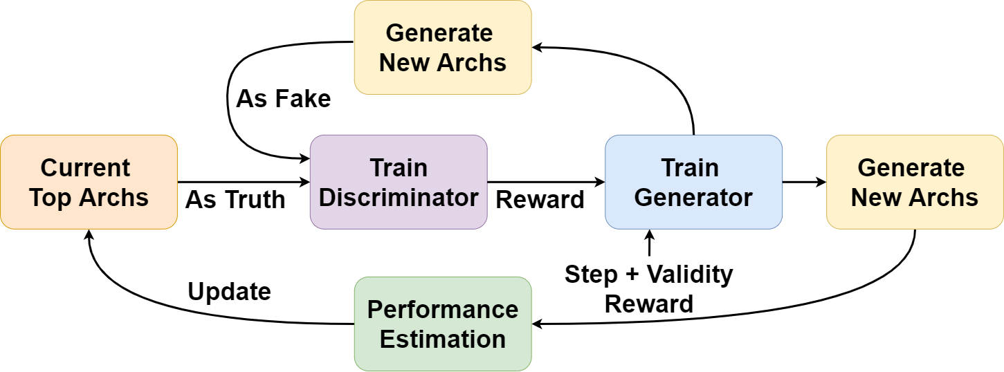
Figure 1: The flow of the proposed GA-NAS algorithm.

3.3 Training Procedure

Generally speaking, in order to solve the minimax problem in Step 4 of Algorithm 1, one can follow the minibatch stochastic gradient descent (SGD) training procedure for training GANs as originally proposed in Goodfellow et al. (2014). However, this SGD approach is not applicable to our case, since the architectures (DAGs) generated by $G$ are discrete samples, and their performance signals cannot be directly back-propagated to update $\theta_{t}$, the parameters of $G$. Therefore, to approximate the JS-divergence minimization between the distribution of top $k$ architectures $\mathcal{T}$, i.e., $p_{\mathcal{T}}$, and the generator distribution $p(x;\theta_{t})$ in iteration $t$, we replace Step 4 of Algorithm 1 by alternately training $D$ and $G$ using a procedure outlined in Algorithm 2. Figure 1 illustrates the overall training flow of GA-NAS.

We first train the GNN-based discriminator using pairs of architectures sampled from $\mathcal{T}$ and $\mathcal{F}$ based on supervised learning. Then, we use Reinforcement Learning (RL) to train $G$ with the reward defined in a similar way as in You et al. (2018), including a step reward that reflects the validity of an architecture during each step of generation and a final reward that mainly comes from the discriminator prediction $D$. When the architecture generation terminates, a final reward $R_{final}$ penalizes the generated architecture $x$ according to the total number of violations of validity or rewards it with a score from the discriminator $D(x)$ that indicates how similar it is to the current true set $\mathcal{T}$. Both rewards together ensure that $G$ generates valid cells that are structurally similar to top cells from the previous time step. We adopt Proximal Policy Optimization (PPO), a policy gradient algorithm with generalized advantage estimation to train the policy, which is also used for NAS in Tan et al. (2019).

Remark.

The proposed learning procedure has several benefits. First, since the generator must sample a discrete architecture $x$ to obtain its discriminator prediction $D(x)$, the entire generator-discriminator pipeline is not end-to-end differentiable and cannot be trained by SGD as in the original GAN. Training $G$ with PPO solves this differentiability issue. Second, in PPO there is an entropy loss term that encourages variations in the generated actions. By tuning the multiplier for the entropy loss, we can control the extent to which we explore a large search space of architectures. Third, using the discriminator outputs as the reward can significantly reduce the number of architecture evaluations compared to a conventional scheme where the fully evaluated network accuracy is used as the reward. Ablation studies in Section 4 verifies this claim. Also refer to the Appendix for a detailed discussion.

Algorithm 2 Training Discriminator $D$ and the Generator $G$

1:Input: Discriminator $D$; Generator $G(x;\theta_{t-1})$; Data set $\mathcal{T}$.

2:for $t^{\prime}=1,2,\ldots,\leavevmode\nobreak\ T^{\prime}$ do

3:     Let $G(x;\theta_{t-1})$ generate $k$ random architectures to form the set $\mathcal{F}$.

4:     Train discriminator $D$ with $\mathcal{T}$ being positive samples and $\mathcal{F}$ being negative samples.

5:     Using the output of $D(x)$ as the main reward signal, train $G(x;\theta_{t})$ with Reinforcement Learning.

6:end for

4 Experimental Results

We evaluate the performance of GA-NAS as a search algorithm by comparing it with a wide range of existing NAS algorithms in terms of convergence speed and stability on NAS benchmarks. We also show the capability of GA-NAS to improve a given network, including already optimized strong baselines such as EfficientNet and ProxylessNAS.

4.1 Results on NAS Benchmarks with or without Weight Sharing

To evaluate search algorithm and decouple it from the impact of search spaces, we query three NAS benchmarks: NAS-Bench-101 Ying et al. (2019), NAS-Bench-201 Dong and Yang (2020), and NAS-Bench-301 Siems et al. (2020). The goal is to discover the highest ranked cell with as few queries as possible. The number of queries to the NAS benchmark is used as a reliable measure for search cost in recent NAS literature Luo et al. (2020); Siems et al. (2020), because each query to the NAS benchmark corresponds to training and evaluating a candidate architecture from scratch, which constitutes the major bottleneck in the overall cost of NAS. By checking the rank an algorithm can reach in a given number of queries, one can also evaluate the convergence speed of a search algorithm. More queries made to the benchmark would indicate a longer evaluation time or higher search cost in a real-world problem.

To further evaluate our algorithm when the true architecture accuracies are unknown, we train a weight-sharing supernet on NAS-Bench-101 and compare GA-NAS with a range of NAS schemes based on weight sharing.

Algorithm	Acc (%)	#Q
Random Search †	93.66	2000
RE †	93.97	2000
NAO †	93.87	2000
BANANAS	94.23	800
SemiNAS †	94.09	2100
SemiNAS †	93.98	300
GA-NAS-setup1	94.22	150
GA-NAS-setup2	94.23	378

Table 1: The best accuracy values found by different search algorithms on NAS-Bench-101 without weight sharing. Note that 94.23% and 94.22% are the accuracies of the 2nd and 3rd best cells. $\dagger$: taken from Luo et al. (2020)

NAS-Bench-101 is the first publicly available benchmark for evaluating NAS algorithms. It consists of 423,624 DAG-style cell-based architectures, each trained and evaluated for 3 times. Metrics for each run include training time and accuracy. Querying NAS-Bench-101 corresponds to evaluating a cell in reality. We provide the results on two setups. In the first setup, we set $|\mathcal{X}_{0}|=50$, $|\mathcal{X}_{t}|=|\mathcal{X}_{t-1}|+50,\leavevmode\nobreak\ t\geq 1$, and $k=25$, In the second setup, we set $|\mathcal{X}_{0}|=100$, $|\mathcal{X}_{t}|=|\mathcal{X}_{t-1}|+100,\leavevmode\nobreak\ t\geq 1$, and $k=50$. For both setups, the initial set $\mathcal{X}_{0}$ is picked to be a random set, and the number of iterations $T$ is 10. We run each setup with 10 random seeds and the search cost for a run is 8 GPU hours on GeForce GTX 1080 Ti.

Algorithm	Mean Acc ($\%$)	Mean Rank	Average #Q
Random Search	93.84 $\pm$ 0.13	498.80	648
Random Search	93.92 $\pm$ 0.11	211.50	1562
GA-NAS-Setup1	94.22 $\pm$ 4.45e-5	2.90	647.50 $\pm$ 433.43
GA-NAS-Setup2	94.23 $\pm$ 7.43e-5	2.50	1561.80 $\pm$ 802.13

Table 2: The average statistics of the best cells found on NAS-Bench-101 without weight sharing, averaged over 10 runs (with std shown). Note that we set the number of queries (#Q) for Random Search to be the same as the average number of queries incurred by GA-NAS.

Table 1 compares GA-NAS to other methods for the best cell that can be found by querying NAS-Bench-101, in terms of the accuracy and the rank of this cell in NAS-Bench-101, along with the number of queries required to find that cell. Table 2 shows the average performance of GA-NAS in the same experiment over multiple random seeds. Note that Table 1 does not list the average performance of other methods except Random Search, since all the other methods in Table 1 only reported their single-run performance on NAS-Bench-101 in their respective experiments.

In both tables, we find that GA-NAS can reach a higher accuracy in fewer number of queries, and beats the best published results, i.e., BANANAS White et al. (2019) and SemiNAS Luo et al. (2020) by an obvious margin. Note that 94.22 is the 3rd best cell while 94.23 is the 2nd best cell in NAS-Bench-101. From Table 2, we observe that GA-NAS achieves superior stability and reproducibility: GA-NAS-setup1 consistently finds the 3rd best in 9 runs and the 2nd best in 1 run out of 10 runs; GA-NAS-setup2 finds the 2nd best in 5 runs and the 3rd best in the other 5 runs.

To evaluate GA-NAS when true accuracy is not available, we train a weight-sharing supernet on the search space of NAS-Bench-101 (with details provided in Appendix) and report the true test accuracies of architectures found by GA-NAS. We use the supernet to evaluate the accuracy of a cell on a validation set of 10k instances of CIFAR10 (see Appendix). Search time including supernet training is around 2 GPU days.

Algorithm	Mean Acc	Best Acc	Best Rank
DARTS †	92.21 $\pm$ 0.61	93.02	57079
NAO †	92.59 $\pm$ 0.59	93.33	19552
ENAS †	91.83 $\pm$ 0.42	92.54	96939
GA-NAS	92.80 $\pm$ 0.54	93.46	5386

Table 3: Searching on NAS-Bench-101 with weight-sharing, with the mean test accuracy of the best cells from 10 runs, and the best accuracy/rank found by a single run. $\dagger$: taken from Yu et al. (2019)

We report results of 10 runs in Table 3, in comparison to other weight-sharing NAS schemes reported in Yu et al. (2019). We observe that using a supernet degrades the search performance in general as compared to true evaluation, because weight-sharing often cannot provide a completely reliable performance for the candidate architectures. Nevertheless, GA-NAS outperforms other approaches.

[hb] CIFAR-10 CIFAR-100 ImageNet-16-120 Algorithm Mean Acc Rank #Q Mean Acc Rank #Q Mean Acc Rank #Q REA ^$\dagger$ 93.92 $\pm$ 0.30 - - 71.84 $\pm$ 0.99 - - 45.54 $\pm$ 1.03 - - RS ^$\dagger$ 93.70 $\pm$ 0.36 - - 71.04 $\pm$ 1.07 - - 44.57 $\pm$ 1.25 - - REINFORCE ^$\dagger$ 93.85 $\pm$ 0.37 - - 71.71 $\pm$ 1.09 - - 45.24 $\pm$ 1.18 - - BOHB ^$\dagger$ 93.61 $\pm$ 0.52 - - 70.85 $\pm$ 1.28 - - 44.42 $\pm$ 1.49 - - RS-500 94.11 $\pm$ 0.16 30.81 500 72.54 $\pm$ 0.54 30.89 500 46.34 $\pm$ 0.41 34.18 500 GA-NAS 94.34 $\pm$ 0.05 4.05 444 73.28 $\pm$ 0.17 3.25 444 46.80 $\pm$ 0.29 7.40 445

• $\dagger$ The results are taken directly from NAS-Bench-201 Dong and Yang (2020).

Table 4: Searching on NAS-Bench-201 without weight sharing, with the mean accuracy and rank of the best cell found reported. #Q represents the average number of queries per run. We conduct 20 runs for GA-NAS.

4.1.1 NAS-Bench-201

This search space contains 15,625 evaluated cells. Architecture cells consist of 6 searchable edges and 5 candidate operations. We test GA-NAS on NAS-Bench-201 by conducting 20 runs for CIFAR-10, CIFAR-100, and ImageNet-16-120 using the true test accuracy. We compare against the baselines from the original NAS-Bench-201 paper Dong and Yang (2020) that are also directly querying the benchmark data. Since no information on the rank achieved and the number of queries is reported for these baselines, we also compare GA-NAS to Random Search (RS-500), which evaluates 500 unique cells in each run. Table 4 presents the results. We observe that GA-NAS outperforms a wide range of baselines, including Evolutionary Algorithm (REA), Reinforcement Learning (REINFORCE), and Bayesian Optimization (BOHB), on the task of finding the most accurate cell with much lower variance. Notably, on ImageNet-16-120, GA-NAS outperforms REA by nearly $1.3$% on average.

Compared to RS-500, GA-NAS finds cells that are higher ranked while only exploring less than 3.2% of the search space in each run. It is also worth mentioning that in the $20$ runs on all three datasets, GA-NAS can find the best cell in the entire benchmark more than once. Specifically for CIFAR-10, it found the best cell in 9 out of 20 runs.

4.1.2 NAS-Bench-301

This is another recently proposed benchmark based on the same search space as DARTS. Relying on surrogate performance models, NAS-Bench-301 reports the accuracy of $10^{18}$ unique cells. We are especially interested in how the number of queries (#Q) needed to find an architecture with high accuracy scales in a large search space. We run GA-NAS on NAS-Bench-301 v0.9. We compare with Random (RS) and Evolutionary (EA) search baselines. Figure 2 plots the average best accuracy along with the accuracy standard deviations versus the number of queries incurred under the three methods. We observe that GA-NAS outperforms RS at all query budgets and outperforms EA when the number of queries exceeds 3k. The results on NAS-Bench-301 confirm that for GA-NAS, the number of queries (#Q) required to find a good performing cell scales well as the size of the search space increases. For example, on NAS-Bench-101, GA-NAS usually needs around 500 queries to find the 3rd best cell, with an accuracy $\approx 94\%$ among 423k candidates, while on the huge search space of NAS-Bench-301 with up to $10^{18}$ candidates, it only needs around 6k queries to find an architecture with accuracy approximately equal to $95\%$.

In contrast to GA-NAS, EA search is less stable and does not improve much as the number of queries increases over 3000. GA-NAS surpasses EA for #Q $\geq 3000$ in Figure 2. What is more important is that the variance of GA-NAS is much lower than the variance of the EA solution over all ranges of #Q. Even though for #Q < 3000, GA-NAS and EA are close in terms of average performance, EA suffers from a huge variance.

Figure 2: NAS-Bench-301 results comparing the means/standard deviations of the best accuracy found at various total query limits.

4.1.3 Ablation Studies

A key question one might raise about GA-NAS is how much the discriminator contributes to the superior search performance. Therefore, we perform an ablation study on NAS-Bench-101 by creating an RL-NAS algorithm for comparison. RL-NAS removes the discriminator in GA-NAS and directly queries the accuracy of a generated cell from NAS-Bench-101 as the reward for training. We test the performance of RL-NAS under two setups that differ in the total number of queries made to NAS-Bench-101. Table 5 reports the results.

Algorithm	Avg. Acc	Avg. Rank	Avg. #Q
RL-NAS-1	94.14 $\pm$ 0.10	20.8	7093 $\pm$ 3904
RL-NAS-2	93.78 $\pm$ 0.14	919.0	314 $\pm$ 300
GA-NAS-Setup1	94.22$\pm$ 4.5e-5	2.9	648 $\pm$ 433
GA-NAS-Setup2	94.23$\pm$ 7.4e-5	2.5	1562 $\pm$ 802

Table 5: Results of ablation study on NAS-Bench-101 by removing the discriminator and directly queries the benchmark for reward.

Compared to GA-NAS-Setup2, RL-NAS-1 makes 3$\times$ more queries to NAS-Bench-101, yet cannot outperform either of the GA-NAS setups. If we instead limits the number of queries as in RL-NAS-2 then the search performance deteriorates significantly. Therefore, we conclude that the discriminator in GA-NAS is crucial for reducing the number of queries, which converts to the number of evaluations in real-world problems, as well as for finding architectures with better performance. Interested readers are referred to Appendix for more ablation studies as well as the Pareto Front search results.

4.2 Improving Existing Neural Architectures

[hb] ResNet Algorithm Best Acc Train Seconds #Weights (M) Hand-crafted 93.18 2251.6 20.35 Random Search 93.84 1836.0 10.62 GA-NAS 93.96 1993.6 11.06 Inception Algorithm Best Acc Train Seconds #Weights (M) Hand-crafted 93.09 1156.0 2.69 Random Search 93.14 1080.4 2.18 GA-NAS 93.28 1085.0 2.69

Table 6: Constrained search results on NAS-Bench-101. GA-NAS can find cells that are superior to the ResNet and Inception cells in terms of test accuracy, training time, and the number of weights.

We now demonstrate that GA-NAS can improve existing neural architectures, including ResNet and Inception cells in NAS-Bench-101, EfficientNet-B0 under hard constraints, and ProxylessNAS-GPU Cai et al. (2018) in unconstrained search.

For ResNet and Inception cells, we use GA-NAS to find better cells from NAS-Bench-101 under a lower or equal training time and number of weights. This can be achieved by enforcing a hard constraint in choosing the truth set $\mathcal{T}$ in each iteration. Table 6 shows that GA-NAS can find new, dominating cells for both cells, showing that it can enforce ad-hoc constraints in search, a property not enforceable by regularizers in prior work. We also test Random Search under a similar number of queries to the benchmark under the same constraints, which is unable to outperform GA-NAS.

We now consider well-known architectures found on ImageNet i.e., EfficientNet-B0 and ProxylessNAS-GPU, which are already optimized strong baselines found by other NAS methods. We show that GA-NAS can be used to improve a given architecture in practice by searching in its original search space.

For EfficientNet-B0, we set the constraint that the found networks all have an equal or lower number of parameters than EfficientNet-B0. For the ProxylessNAS-GPU model, we simply put it in the starting truth set and run an unconstrained search to further improve its top-1 validation accuracy. More details are provided in the Appendix. Table 7 presents the improvements made by GA-NAS over both existing models. Compared to EfficientNet-B0, GA-NAS can find new single-path networks that achieve comparable or better top-1 accuracy on ImageNet with an equal or lower number of trainable weights. We report the accuracy of EfficientNet-B0 and the GA-NAS variants without data augmentation. Total search time including supernet training is around 680 GPU hours on Tesla V100 GPUs. It is worth noting that the original EfficientNet-B0 is found using the MNasNet Tan et al. (2019) with a search cost over 40,000 GPU hours.

Network	#Params	Top-1 Acc
EfficientNet-B0 (no augment)	$5.3$M	$76.7$
GA-NAS-ENet-1	4.6M	$76.5$
GA-NAS-ENet-2	5.2M	76.8
GA-NAS-ENet-3	$5.3$M	76.9
ProxylessNAS-GPU	$4.4$M	$75.1$
GA-NAS-ProxylessNAS	$4.9$M	75.5

Table 7: Results on the EfficientNet and ProxylessNAS spaces.

For ProxylessNAS experiments, we train a supernet on ImageNet and conduct an unconstrained search using GA-NAS for 38 hours on 8 Tesla V100 GPUs, a major portion of which, i.e., 29 hours is spent on querying the supernet for architecture performance. Compared to ProxylessNAS-GPU, GA-NAS can find an architecture with a comparable number of parameters and a better top-1 accuracy.

5 Conclusion

In this paper, we propose Generative Adversarial NAS (GA-NAS), a provably converging search strategy for NAS problems, based on generative adversarial learning and the importance sampling framework. Based on extensive search experiments performed on NAS-Bench-101, 201, and 301 benchmarks, we demonstrate the superiority of GA-NAS as compared to a wide range of existing NAS methods, in terms of the best architectures discovered, convergence speed, scalability to a large search space, and more importantly, the stability and insensitivity to random seeds. We also show the capability of GA-NAS to improve a given practical architecture, including already optimized ones either manually designed or found by other NAS methods, and its ability to search under ad-hoc constraints. GA-NAS improves EfficientNet-B0 by generating architectures with higher accuracy or lower numbers of parameters, and improves ProxylessNAS-GPU with enhanced accuracies. These results demonstrate the competence of GA-NAS as a stable and reproducible search algorithm for NAS.

Appendix A Appendix

A.1 Importance Sampling and the Cross-Entropy Method

Assume $X$ is a random variable, taking values in $\mathcal{X}$ and has a prior probability density function (pdf) $p(.;\bar{\lambda})$ for fixed $\bar{\lambda}\in\Theta$. Let $S(X)$ be the objective function to be maximized, and $\alpha$ be a level parameter. Note that the event $\mathcal{E}:=\left\{S(X)\geq\alpha\right\}$ is a rare event for an $\alpha$ that is equal to or close to the optimal value of $S(X)$. The goal of rare-event probability estimation is to estimate

$$l(\alpha) := \mathbb{P}_{\bar{\lambda}}\left(S(X)\geq\alpha\right)$$

$$= \mathbb{E}_{\bar{\lambda}}\left[\mathbb{I}_{S(X)\geq\alpha}\right]=\int\mathbb{I}_{S(x)\geq\alpha}\leavevmode\nobreak\ p(x;\bar{\lambda})dx,$$

where $\mathbb{I}_{x\in\mathcal{E}}$ is an indicator function that is equal to 1 if $x\in\mathcal{E}$ and 0 otherwise.

In fact, $l(\alpha)$ is called the rare-event probability (or expectation) which is very small, e.g., less than $10^{-4}$. The general idea of importance sampling is to estimate the above rare-event probability $l$ by drawing samples $x$ from important regions of the search space with both a large density $p(x;\bar{\lambda})$ and a large $\mathbb{I}_{S(x)\geq\alpha}$, i.e., $\mathbb{I}_{S(x)\geq\alpha}=1$. In other words, we aim to find $x$ such that $S(x)\geq\alpha$ with high probability.

Importance sampling estimates $l$ by sampling $x$ from a distribution $q^{*}(x,\alpha;\bar{\lambda})$ that should be proportional to $\mathbb{I}_{S(x)\geq\alpha}p(x;\bar{\lambda})$. Specifically, define the proposal sampling density $q(x)$ as a function such that $q(x)=0$ implies $\mathbb{I}_{S(x)\geq\alpha}p(x;\bar{\lambda})=0$ for every $x$. Then we have

$$l(\alpha)=\int\frac{\mathbb{I}_{S(x)\geq\alpha}p(x;\bar{\lambda})}{q(x)}q(x)dx=\mathbb{E}_{q}\left[\frac{\mathbb{I}_{S(X)\geq\alpha}p(X;\bar{\lambda})}{q(X)}\right].$$ (1)

Rubinstein and Kroese [2013] shows that the optimal importance sampling probability density $q$ which minimizes the variance of the empirical estimator of $l(\alpha)$ is the density of $X$ conditional on the event $S(X)\geq\alpha$, that is

$$q^{*}(x,\alpha;\bar{\lambda})=\frac{p(x;\bar{\lambda})\mathbb{I}_{S(x)\geq\alpha}}{\int\mathbb{I}_{S(x)\geq\alpha}\leavevmode\nobreak\ p(x;\bar{\lambda})dx}.$$ (2)

However, noting that the denominator of (2) is the quantity $l(\alpha)$ that we aim to estimate in the first place, we cannot obtain an explicit form of $q^{*}(.)$ directly. To overcome this issue, the CE method Homem-de Mello and Rubinstein [2002] aims to choose the sampling probability density $q(.)$ from the parametric families of densities $\{p(.;\theta)\}$ such that the Kullback-Leibler (KL)-divergence between the optimal importance sampling probability density $q^{*}(.,\alpha;\bar{\lambda})$, given by (2), and $p(.;\theta)$ is minimized.

The CE-Optimal solution $\theta^{*}$ is given by

$$\theta^{*} = \arg\min_{\theta}KL\left(q^{*}(.,\alpha;\bar{\lambda})||p(.;\theta)\right)$$ (3)

$$= \arg\max_{\theta}\mathbb{E}_{\bar{\lambda}}\left[\mathbb{I}_{S(X)\geq\alpha}\ln p(X;\theta)\right]$$

$$= \arg\max_{\theta}\mathbb{E}_{\tilde{\theta}}\left[\mathbb{I}_{S(X)\geq\alpha}\ln p(X;\theta)\frac{p(X;\bar{\lambda})}{p(X;\tilde{\theta})}\right],$$

given any prior sampling distribution parameter $\tilde{\theta}\in\Theta$. Let $x_{1},\ldots,x_{N}$ be i.i.d samples from $p(.;\tilde{\theta})$. Then an empirical estimate of $\theta^{*}$ is given by

$$\hat{\theta^{*}}=\arg\max_{\theta}\frac{1}{N}\sum_{k=1}^{N}\mathbb{I}_{S(x_{k})\geq\alpha}\frac{p(x_{k};\bar{\lambda})}{p(x_{k};\tilde{\theta})}\ln p(x_{k};{\theta}).$$ (4)

In the case of rare events, where $l(\alpha)\leq 10^{-6}$, solving the optimization problem (4) does not help us estimate the probability of the rare event (see Homem-de Mello and Rubinstein [2002]). Algorithm 3 presents the multi-stage CE approach proposed in Homem-de Mello and Rubinstein [2002] to overcome this problem. This iterative CE algorithm essentially creates a sequence of sampling probability densities $p(.;\theta_{1}),p(,;\theta_{2}),\ldots$ that are steered toward the direction of the theoretically optimal density $q^{*}(.,\alpha;\bar{\lambda})$ in an iterative manner.

Algorithm 3 CE Method for rare-event estimation

1:Input: Level parameter $\alpha>0$, some fixed parameter $\delta>0$, and initial parameters $\bar{\lambda}$ and $\rho$.

2:$t\leftarrow 1$, $\rho_{0}\leftarrow\rho$, $\theta_{0}\leftarrow\bar{\lambda}$

3:while $\gamma(\theta_{t-1},\rho_{t-1})<\alpha$ do

4:     $\gamma_{t-1}\leftarrow\min(\alpha,\gamma(\theta_{t-1},\rho_{t-1}))$

5:     

$$\begin{multlined}\theta_{t}\in\arg\max_{\theta\in\Theta}\mathbb{E}_{\bar{\lambda}}\left[\mathbb{I}_{S(X)\geq\gamma_{t-1}}\ln p(X;\theta)\right]\\ =\arg\min_{\theta\in\Theta}KL(q^{*}(.,\gamma_{t-1};\bar{\lambda})||p(.;\theta))\end{multlined}\theta_{t}\in\arg\max_{\theta\in\Theta}\mathbb{E}_{\bar{\lambda}}\left[\mathbb{I}_{S(X)\geq\gamma_{t-1}}\ln p(X;\theta)\right]\\ =\arg\min_{\theta\in\Theta}KL(q^{*}(.,\gamma_{t-1};\bar{\lambda})||p(.;\theta))$$

6:     Set $\rho_{t}$ such that $\gamma(\theta_{t},\rho_{t})\geq\min(\alpha,\gamma(\theta_{t-1},\rho_{t-1})+\delta)$.

7:     $t\leftarrow t+1$.

8:end while

More precisely, in Algorithm 3, we denote the threshold sequence by ${\gamma_{t}}$ for $t\geq 0$, and sampling distribution parameters by $\theta_{t}$ for $t\geq 0$. Initially, choose $\rho$ and $\gamma(\bar{\lambda},\rho)$ so that $\gamma(\bar{\lambda},\rho)$ is the $(1-\rho)$-quantile of $S(X)$ under the density $p(.;\bar{\lambda})$, and generally, let $\gamma(\theta_{t},\rho_{t})$ be the $(1-\rho_{t})$-quantile of $S(X)$ under the sampling density $p(x;\theta_{t})$ of iteration $t$. Furthermore, the a priori sampling density parameter $\tilde{\theta}$ introduced in (3) and (4) is replaced by the optimum parameter obtained in iteration $t-1$, i.e., $\theta_{t-1}$.

From (3), we notice that Step 4 in Algorithm 3 is equivalent to minimizing the KL-divergence between the following two densities, $q(x,\gamma_{t-1};\bar{\lambda})=c^{-1}\mathbb{I}_{S(x)\geq\gamma_{t-1}}p(x;\bar{\lambda})$ and $p(x;\theta)$, where $c=\int\mathbb{I}_{S(x)\geq\gamma_{t-1}}p(x;\bar{\lambda})dx$, $\gamma_{t-1}=\min(\alpha,\gamma(\theta_{t-1},\rho_{t-1}))$. One can always choose a small $\delta$ in Step 5, which will determine the number of times the while loop is executed.

The following theorem which was first proved by Homem-de Mello and Rubinstein [2002] asserts that Algorithm 3 terminates. We provide a proof of Theorem A.1 as follows.

Theorem A.1.

Assume that $l(\alpha)>0$. Then, Algorithm 3 converges to a CE-optimal solution in a finite number of iterations.

Proof.

Let $t$ be an arbitrary iteration of the algorithm, and let $\rho_{\alpha}:=P(S(X)\geq\alpha;\theta_{t})$. It can be shown by induction that $\rho_{\alpha}>0$. Note that this is also true if $p(x;\theta)>0$ for all $\theta,x$. Next, we show that for every $\rho_{t}\in(0,\rho_{\alpha})$, $\gamma(\theta_{t},\rho_{t})\geq\alpha$. By the definition of $\gamma$, we have

$$P(S(X)\geq\gamma(\theta_{t},\rho_{t});\theta)\geq\rho_{t},$$

$$P(S(X)\leq\gamma(\theta_{t},\rho_{t});\theta)\geq 1-\rho_{t}>1-\rho_{\alpha}.$$ (5)

Suppose by contradiction, that $\gamma(\theta_{t},\rho_{t})<\alpha$. Then, we get

$$P(S(X)\leq\gamma(\theta_{t},\rho_{t});\theta^{*})\leq P(S(X)\leq\alpha;\theta_{t})=1-\rho_{\alpha},$$

which contradicts (A.1). Thus, $\gamma(\theta_{t},\rho_{t})\geq\alpha$. This implies that Step 5 can always be carried out for any $\delta>0$. Consequently, Algorithm 3 terminates after $T$ iterations with $T\leq\lceil\alpha/\delta\rceil$. Thus at time $T$, we have

$$\theta_{T}\in\operatorname*{arg\,max}_{\theta\in\Theta}\mathbb{E}_{\bar{\lambda}}\left[\mathbb{I}_{S(X)\geq\alpha}\ln P(X;\theta)\right],$$

which implies that $\theta_{T}$ is a CE-Optimal solution. Therefore, Algorithm 3 converges to a CE-Optimal solution in a finite number of iterations. ∎

A.2 Proof of Theorem 3.1

Proof of Theorem 3.1.

Let $p(x;\bar{\lambda})$ be the initial sampling distribution over the initial set of architectures $\mathcal{X}_{0}$. We can consider $\gamma_{0}$ to be the $(1-\rho)$-quantile under $p(x;\bar{\lambda})$. Then, we can consider $\rho$, $\delta>0$ and $\bar{\lambda}$ to be the inputs to Algorithm 3 of Section A.1. Furthermore, by having $\gamma_{t}>=\min(\alpha,\gamma_{t-1}+\delta)$, we can view $\gamma_{t}$ as the $(1-\rho_{t})$-quantile under the sampling density $p(x;\theta_{t})$ provided by the generator $G(.;\theta_{t})$ at the $t$-th iteration, for all $t\in\{1,\ldots,T\}$.

We now modify Algorithm 3 of Section A.1 by replacing the KL-divergence minimization of Step 5 of Algorithm 3 with minimizing the Jensen-Shannon (JS)-divergence to obtain Algorithm 4 for JS-divergence minimization for rare event simulation. Note that Step 4 of Algorithm 4 is equivalent to Step 4 of Algorithm 1. Furthermore, the distribution of architectures in $\mathcal{T}$, i.e., the distribution of top architectures in prior iteration in Algorithm 1, corresponds to $q(x,\gamma_{t-1};\bar{\lambda})$ in Algorithm 4. By choosing $k$ such that $k=\rho_{t}\times|\bigcup_{i=0}^{t-1}\mathcal{X}_{i}|$ and the above argument, we note that Algorithm 4 and Algorithm 1 are equivalent. Therefore, by showing that Algorithm 4 converges in a finite number of iterations, we imply that Algorithm 1 converges in a finite number of iterations.

Using the convergence result of Algorithm 3, we now show that Algorithm 4 converges in a finite number of iterations.

Consider the JS divergence between $q(x,\gamma_{t-1};\bar{\lambda})=c^{-1}\mathbb{I}_{S(x)\geq\gamma_{t-1}}p(x;\bar{\lambda})$ and $p(x;\theta)$, where $c=\int\mathbb{I}_{S(x)\geq\gamma_{t-1}}p(x;\bar{\lambda})dx$, $\gamma_{t-1}=\min(\alpha,\gamma(\theta_{t-1},\rho_{t-1}))$, which is

$$JS(q(x,\gamma_{t-1};\bar{\lambda})||p(x;\theta))=$$

$$\frac{1}{2}KL(c^{-1}p(x;\bar{\lambda})\mathbb{I}_{S(X)\geq\gamma_{t-1}}\parallel$$

$$\frac{1}{2}\left(c^{-1}p(x;\bar{\lambda})\mathbb{I}_{S(X)\geq\gamma_{t-1}}+p(x;\theta))\right)+$$

$$\frac{1}{2}KL(p(x;\theta)\parallel\frac{1}{2}(c^{-1}p(x;\bar{\lambda})\mathbb{I}_{S(X)\geq\gamma_{t-1}}+$$

$$p(x;\theta))).$$ (6)

We say $\theta^{*}$ is a JS-optimal solution, if

$$\theta^{*}\in\arg\min_{\theta\in\Theta}JS(q(x,\gamma_{t-1};\bar{\lambda})||p(x;\theta)).$$ (7)

Algorithm 4 JS-divergence minimization for rare-event estimation

1:Input: Level parameter $\alpha>0$, some fixed parameter $\delta>0$, and initial parameters $\bar{\lambda}$ and $\rho$.

2:$t\leftarrow 1$, $\rho_{0}\leftarrow\rho$, $\theta_{0}\leftarrow\bar{\lambda}$

3:while $\gamma(\theta_{t-1},\rho_{t-1})<\alpha$ do

4:     $\theta_{t}\in\arg\min_{\theta\in\Theta}JS(q(x,\gamma_{t-1};\bar{\lambda})||p(x;\theta))$, where $\gamma_{t-1}=\min(\alpha,\gamma(\theta_{t-1},\rho_{t-1}))$ and

$$q(x,\gamma_{t-1};\bar{\lambda})=\frac{\mathbb{I}_{S(x)\geq\gamma_{t-1}}p(x;\bar{\lambda})}{\int\mathbb{I}_{S(x)\geq\gamma_{t-1}}p(x;\bar{\lambda})dx}.$$

5:     Set $\rho_{t}$ such that $\gamma(\theta_{t},\rho_{t})\geq\min(\alpha,\gamma(\theta_{t-1},\rho_{t-1})+\delta)$.

6:     $t\leftarrow t+1$.

7:end while

The assumption that $\max_{x\in\mathcal{X}}S(x)\geq\alpha$, for some $\alpha>0$, implies the assumption of Theorem A.1, i.e., $l(\alpha)>0$. Then, following the same arguments as in the proof of Theorem A.1, the assertion of Theorem A.1 still holds for the case of JS-divergence minimization of Algorithm 4, and consequently, Algorithm 1 converges to a JS-optimal solution in a finite number of iterations. ∎

A.3 Model Details

A.3.1 Pairwise Architecture Discriminator

Consider the case where we search for a cell architecture $\mathcal{C}$, the input to $D$ is a pair of cells $(\mathcal{C}^{true},\mathcal{C}^{\prime})$, where $\mathcal{C}^{true}$ denotes a cell from the current truth data, while $\mathcal{C}^{\prime}$ is a cell from either the truth data or the generator’s learned distribution. We transform each cell in the pair into a graph embedding vector using a shared $k$-GNN model. The graph embedding vectors of the input cells are then concatenated and passed to an MLP for classification. We train $D$ in a supervised fashion and minimize the cross-entropy loss between the target labels and the predictions. To create the training data for $D$, we first sample $\mathcal{T}$ unique cells from the current truth data. We create positive training samples by pairing each truth cell against every other truth cell. We then let the generator generate $|\mathcal{T}|$ unique and valid cells as fake data and pair each truth cell against all the generated cells.

A.3.2 Architecture Generator

A complete architecture is constructed in an auto-regressive fashion. We define the state at the $t$-th time step as ${\mathcal{C}}_{t}$, which is a partially constructed graph. Given the state ${\mathcal{C}}_{t-1}$, the actor inserts a new node. The action $a_{t}$ is composed of an operator type for this new node selected from a predefined operation space and its connections to previous nodes. We define an episode by a trajectory $\tau$ of length $N$ as the state transitions from ${\mathcal{C}}_{0}$ to ${\mathcal{C}}_{N-1}$, i.e., $\tau=\{{\mathcal{C}}_{0},{\mathcal{C}}_{1},\ldots,{\mathcal{C}}_{N-1}\}$, where $N$ is an upper bound that limits the number of steps allowed in graph construction. The actor model follows an Encoder-Decoder framework, where the encoder is a multi-layer $k$-GNN. The decoder consists of an MLP and a Gated Recurrent Unit. The architecture construction terminates when the actor generates a terminal output node or the final state ${\mathcal{C}}_{N-1}$ is reached. Figure 3 illustrates an architecture generator used in our NAS-Bench-101 experiments.

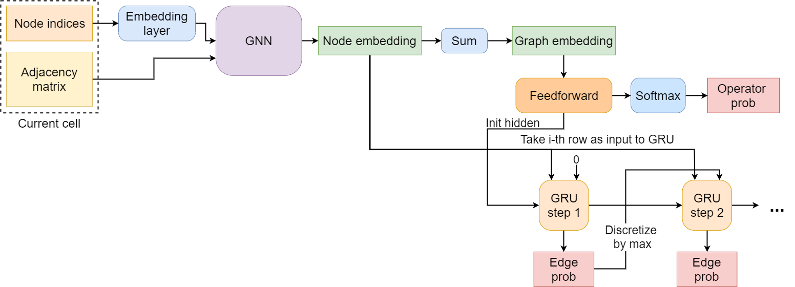
Figure 3: The structure of a GNN architecture generator for cell-based micro search.

A.3.3 Training Procedure of the Architecture Generator

The state transition is captured by a policy $\pi_{\theta}(a_{t}|{\mathcal{C}}_{t})$, where the action $a_{t}$ includes predictions on a new node type and its connections to previous nodes. To learn $\pi_{\theta}(a_{t}|{\mathcal{C}}_{t})$ in this discrete action space, we adopt the Proximal Policy Optimization (PPO) algorithm with generalized advantage estimation. The actor is trained by maximizing the cumulative expected reward of the trajectory. For a trajectory $\tau$ with a maximum allowed length of $N$, this objective translates to

$$\begin{split}\max E[R(\tau)]=\max E[R_{step}(\tau)]+E[R_{final}(\tau)]\\ \quad\textrm{s.t. }|\tau|\leq N,\end{split}$$ (8)

where $R_{step}$ and $R_{final}$ correspond the per-step reward and the final reward, respectively, which will be described in the following.

In the context of cell-based micro search, there is a step reward $R_{step}$, which is given to the actor after each action, and a final reward $R_{final}$, which is only assigned at the end of a multi-step generation episode. For $R_{step}$, we assign the generator a step reward of $0$ if $a_{t}$ is valid. Otherwise, we assign $-0.1$ and terminate the episode immediately.

$R_{final}$ consists of two parts. The first part is a validity score $R_{v}$. For a completed cell $\mathcal{C}_{gen}$, if it is a valid DAG and contains exactly one output node, and there is at least one path from every other node to the output, then the actor receives a validity score of $R_{v}(\mathcal{C}_{gen})=0$. Otherwise, the validity score will be $-0.1$ multiplied by the number of validity violations. In our search space, we define four possible violations: 1) There is no output node; 2) There is a node with no incoming edges; 3) There is a node with no outgoing edges; 4) There is a node with no incoming or outgoing edges. The second part of $R_{final}$ is $R_{D}(\mathcal{C}_{gen})$, which represents the probability that the discriminator classifies $\mathcal{C}_{gen}$ as a cell from the truth data distribution $p_{data}(x)$. In order to receive $R_{D}(\mathcal{C}_{gen})$ from the discriminator, $\mathcal{C}_{gen}$ must have a validity score of $0$ and $\mathcal{C}_{gen}$ cannot be one of the current truth cells $\{\mathcal{C}^{j}_{true}|j=1,2,...K\}$.

Formally, we express the final reward $R_{final}$ for a generated architecture $\mathcal{C}_{gen}$ as

$$R_{final}=\begin{cases}R_{v}(\mathcal{C}_{gen})&\mbox{if }I(C_{gen}),\\ R_{v}(\mathcal{C}_{gen})+R_{D}(\mathcal{C}_{gen})&\mbox{otherwise. }\end{cases}$$ (9)

And $I(C_{gen})=R_{v}(\mathcal{C}_{gen})<0\textrm{ or }\mathcal{C}_{gen}\in\{\mathcal{C}^{j}_{true}|j=1,2,...K\}$. We compute $R_{D}(\mathcal{C}_{gen})$ by conducting pairwise comparisons against the current truth cells, then take the maximum probability that the discriminator will predict a $1$, i.e., $R_{D}=\max_{j}\textrm{ }P(\mathcal{C}_{gen}\in p_{data}(x)|\mathcal{C}_{gen},\mathcal{C}^{j}_{true};D),\textrm{ for }j=1,2,...K$, as the discriminator reward.

Maintaining the right balance of exploration/exploitation is crucial for a NAS algorithm. In GA-NAS, the architecture generator and discriminator provide an efficient way to utilize learned knowledge, i.e., exploitation. For exploration, we make sure that the generator always have some uncertainties in its actions by tuning the multiplier for the entropy loss in the PPO learning objective. The entropy loss determines the amount of randomness, hence, variations in the generated actions. Increasing its multiplier would increase the impact of the entropy loss term, which results in more exploration. In our experiments, we have tuned this multiplier extensively and found that a value of $0.1$ works well for the tested search spaces.

Last but not least, it is worth mentioning that the above formulation of the reward function also works for the single-path macro search scenario, such as EfficientNet and ProxylessNAS search spaces, in which we just need to modify $R_{step}$ and $R_{D}(\mathcal{C}_{gen})$ according to the definitions of the new search space.

A.4 Experimentation

In this section, we present ablation studies and the results of additional experiments. We also provide more details on our experimental setup. We implement GA-NAS using PyTorch 1.3. We also use the PyTorch Geometric library for the implementation of $k$-GNN.

A.4.1 More Ablation Studies

We report the results of ablation studies to show the effect of different components of GA-NAS on its performance.

Standard versus Pairwise Discriminator: In order to investigate the effect of pairwise discriminator in GA-NAS explained in section 3, we perform the same experiments as in Table 2, with the standard discriminator where each architecture $\in\mathcal{T}$ is compared against a generated architecture $\in\mathcal{F}$. The results presented in Table 8 indicate that using pairwise discriminator leads to a better performance compared to using standard discriminator.

Algorithm	Mean Acc	Mean Rank	Average #Q
GA-NAS-Setup1 with pairwise discriminator	94.221$\pm$ 4.45e-5	2.9	647.5 $\pm$ 433.43
GA-NAS-Setup1 without pairwise discriminator	94.22$\pm$ 0.0	3	771.8 $\pm$ 427.51
GA-NAS-Setup2 with pairwise discriminator	94.227$\pm$ 7.43e-5	2.5	1561.8 $\pm$ 802.13
GA-NAS-Setup2 without pairwise discriminator	94.22$\pm$ 0.0	3	897 $\pm$ 465.20

Table 8: The mean accuracy and rank, and average number of queries over 10 runs.

Uniform versus linear sample size increase with fixed number of evaluation budget: Once the generator in Algorithm 1 is trained, we sample $|\mathcal{X}_{t}|$ architectures $\mathcal{X}_{t}$. Intuitively, as the algorithm progresses, $G$ becomes more and more accurate, thus, increasing the size of $\mathcal{X}_{t}$ over the iterations should prove advantageous. We provide some evidence that this is the case. More precisely, we perform the same experiments as in Table 2; however, keeping the total number of generated cell architectures during the 10 iterations of the algorithm the same as that in the setup of Table 2, we generate a constant number of cell architectures of $225$ and $450$ in each iteration of the algorithm in setup1 and setup2, respectively. The results presented in Table 9 indicate that a linear increase in the size of generated cell architectures leads to a better performance.

Algorithm	Mean Acc	Mean Rank	Average #Q
GA-NAS-Setup1 ($|\mathcal{X}_{t}|=|\mathcal{X}_{t-1}|+50,\leavevmode\nobreak\ \forall t\geq 2$)	94.221 $\pm$ 4.45e-5	2.9	647.5 $\pm$ 433.43
GA-NAS-Setup1 ($|\mathcal{X}_{t}|=225,\leavevmode\nobreak\ \forall t\geq 2$)	94.21$\pm$ 0.000262	3.4	987.7 $\pm$ 394.79
GA-NAS-Setup2 ($|\mathcal{X}_{t}|=|\mathcal{X}_{t-1}|+50,\leavevmode\nobreak\ \forall t\geq 2$)	94.227$\pm$ 7.43e-5	2.5	1561.8 $\pm$ 802.13
GA-NAS-Setup2 ($|\mathcal{X}_{t}|=450,\leavevmode\nobreak\ \forall t\geq 2$)	94.22$\pm$ 0.0	3	1127.6 $\pm$ 363.75

Table 9: The mean accuracy and rank, and average number of queries over 10 runs.

A.4.2 Pareto Front Search Results on NAS-Bench-101

In addition to constrained search, we search through Pareto frontiers to further illustrate our algorithm’s ability to learn any given truth set. We consider test accuracy vs. normalized training time and found that the truth Pareto front of NAS-Bench-101 contains 41 cells. To reduce variance, we always initialize with the worst 50% of cells in terms of accuracy and training time, which amounts to 82,329 cells. We modify GA-NAS to take a Pareto neighborhood of size 4 in each iteration, which is defined as iteratively removing the cells in the current Pareto front and finding a new front using the remaining cells, until we have collected cells from 4 Pareto fronts. We run GA-NAS for $10$ iterations and compare with a random search baseline. GA-NAS issued 2,869 unique queries (#Q) to the benchmark, so we set the #Q for random search to 3,000 for a fair comparison. Figure 4 showcases the effectiveness of GA-NAS in uncovering the Pareto front. While random search also finds a Pareto front that is close to the truth, a small gap is still visible. In comparison, GA-NAS discovers a better Pareto front with a smaller number of queries. GA-NAS finds 10 of the 41 cells on the truth Pareto front, and random search only finds 2.

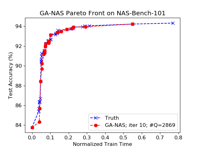
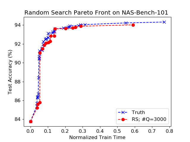
Figure 4: Pareto Front search on NAS-Bench-101. Observe that GA-NAS nearly recovers the truth Pareto Front while Random Search (RS) only discovers one close to the truth. #Q represents the total number of unique queries made to the benchmark. Each marker represents a cell on the Pareto front.

A.4.3 Hyper-parameter Setup

Table 10 reports the key hyper-parameters used in our NAS-Bench-101, 201 and 301 experiments, which includes (1) best-accuracy search by querying the true accuracy (Acc), (2) best-accuracy search using the supernet (Acc-WS), (3) constrained best-accuracy search (Acc-Cons), and (4) Pareto front search (Pareto).

Here, we include a brief description for some parameters in Table 10.

• # Eval base ($|\mathcal{X}_{1}|$) is the number of unique, valid cells to be generated by $G$ after the first iteration of $D$ and $G$ training, i.e., last step of an iteration of Algorithm. 1.

• # Eval inc ($|\mathcal{X}_{t}|-|\mathcal{X}_{t-1}|$) is the increment to the number of generated cells after completing an iteration. From the CE method and importance sampling described in Sec. A.1, the early generator distribution is not close enough to the well-performing cell architecture. To lower the number of queries to the benchmark without sacrificing the performance, we propose an incremental increase in the number of generated cell architectures at each iteration.

• Init method describes how to choose the initial set of cells, from which we create the initial truth set. For most experiments, we randomly choose $|\mathcal{X}_{0}|$ number of cells as the initial set. For the Pareto front search, we initialize with cells that rank in the lower 50% in terms of both test accuracy and training time (which constitutes 82,329 cells in NAS-Bench-101).

• Truth set size ($\mathcal{T}$) controls the number of truth cells for training $D$. For best-accuracy searches, we take the top most accurate cells found so far. For Pareto front searches, we iteratively collect the cells on the current Pareto front, then remove them from the current pool, then find a new Pareto front, until we visit the desired number of Pareto fronts.

For the complete set of hyper-parameters, please check out our code.

[hb] NAS-Bench-101 NAS-Bench-201 NAS-Bench-301 Parameter Acc (2 setups) Acc-WS Acc-Cons Pareto Acc (3 datasets) Acc $G$ optimizer Adam Adam Adam Adam Adam Adam $G$ learn rate 0.0001 0.0001 0.0001 0.0001 0.0001 0.0001 $D$ optimizer Adam Adam Adam Adam Adam Adam $D$ learn rate 0.001 0.001 0.001 0.001 0.001 0.001 # GNN layers 2 2 2 2 2 2 Iterations ($T$) 10 5 5 10 5 10 # Eval base ($|\mathcal{X}_{1}|$) 100 100 200 500 60 50 # Eval inc ($|\mathcal{X}_{t}|-|\mathcal{X}_{t-1}|$) 50, 100 100 200 100 10 50 Init method Random Random Random Worst 50% Random Random Init size ($|\mathcal{X}_{0}|$) 50; 100 100 100 82329 60 100 Truth set size ($|\mathcal{T}|$) 25; 50 50 50 4 fronts 40 50

Table 10: Key hyper-parameters used by our NAS-Bench-101, 201 and 301 experiments. Among multiple runs of an experiment, the same hyper-parameters are used and only the random seed differs.

A.4.4 Supernet Training and Usage

To train a supernet for NAS-Bench-101, we first set up a macro-network in the same way as the evaluation network of NAS-Bench-101. Our supernet has 3 stacks with 3 supercells per stack. A downsampling layer consisting of a Maxpooling 2-by-2 and a Convolution 1-by-1 is inserted after the first and second stack to halve the input width/height and double the channels. Each supercell contains 5 searchable nodes. In a NAS-Bench-101 cell, the output node performs concatenation of the input features. However, this is not easy to handle in a supercell. Therefore, we replace the concatenation with summation and do not split channels between different nodes in a cell.

We train the supernet on 40,000 randomly sampled CIFAR-10 training data and leave the other 10,000 as validation data. We set an initial channel size of 64 and a training batch size of 128. We adopt a uniformly random strategy for training, i.e., for every batch of training data, we first uniformly sample an edge topology, then, we uniformly sample one operator type for every searchable node in the topology. Following this strategy, we train for 500 epochs using the Adam optimizer and an initial learning rate of 0.001. We change the learning rate to 0.0001 when the training accuracy do not improve for 50 consecutive epochs.

During search, after we acquire the set of cells ($\mathcal{X}$) to evaluate, we first fine-tune the current supernet for another 50 epochs. The main difference here compared to training a supernet from scratch is that for a batch of training data, we randomly sample a cell from $\mathcal{X}$ instead of from the complete search space. We use the Adam optimizer with a learning rate of 0.0001. Then, we get the accuracy of every cell in $\mathcal{X}$ by testing on the validation data and by inheriting the corresponding weights of the supernet.

A.4.5 ResNet and Inception Cells in NAS-Bench-101

Figure 5 illustrates the structures of the ResNet and Inception cells used in our constrained best-acc search. Note that both cells are taken from the NAS-Bench-101 database as is, there might be small differences in their structures compared to the original definitions. Table 6 reports that the ResNet cell has a lot more weights than the inception cell, even though it contains fewer operators. This is because NAS-Bench-101 performs channel splitting so that each operator in a branched path will have a much fewer number of trainable weights.

We then present the two best cell structures found by GA-NAS that are better than the ResNet and Inception cells, respectively, in Figure 6. Both cells are also in the NAS-Bench-101 database. Observe that both cells contain multiple branches coming from the input node.

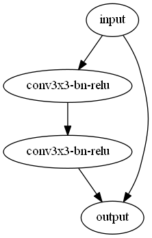
(a) ResNet cell

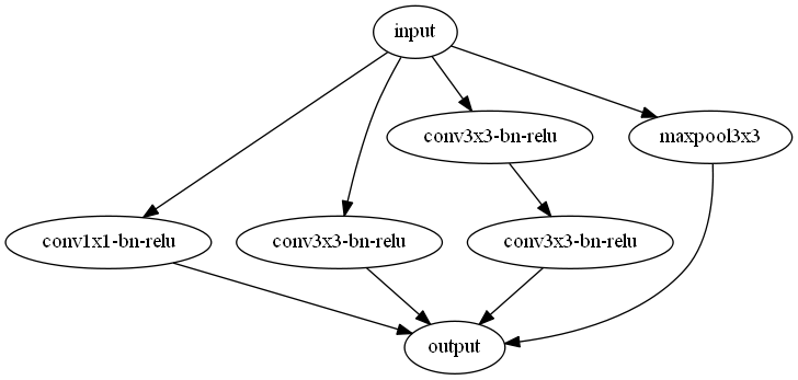
(b) Inception cell

Figure 5: Structures of the ResNet and Inception cells, which are considered hand-crafted architectures in our constrained best-accuracy search.

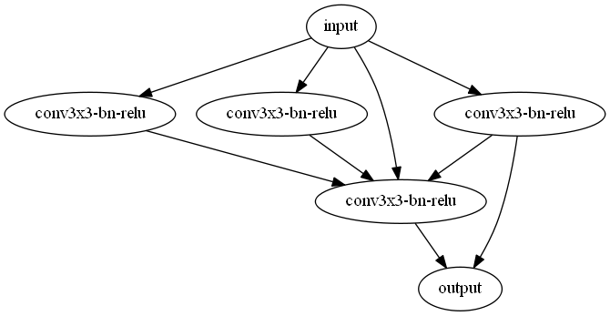
(a) ResNet cell replacement.

(b) Inception cell replacement.

Figure 6: The structures of the best two cells found by GA-NAS that are better than the ResNet and Inception cells in terms of test accuracy, training time and number of weights.

A.4.6 More on NAS-Bench-101 and NAS-Bench-201

We summarize essential statistical information about NAS-Bench-101 and NAS-Bench-201 in Table 11. The purpose is to establish a common ground for comparisons. Future NAS works who wish to compare to our experimental results directly can check Table 11 to ensure a matching benchmark setting. There are 3 candidate operators for NAS-Bench-101, (1) A sequence of convolution 3-by-3, batch normalization (BN), and ReLU activation (Conv3$\times$3-BN-ReLU), (2) Conv1$\times$1-BN-ReLU, (3) Maxpool3$\times$3. NAS-Bench-201 defines 5 operator choices: (1) zeroize, (2) skip connection, (3) ReLU-Conv1$\times$1-BN, (4) ReLU-Conv3$\times$3-BN, (5) Averagepool3$\times$3. We want the re-emphasize that for each cell in NAS-Bench-101, we take the average of the final test accuracy at epoch 108 over 3 runs as its true test accuracy. For NAS-Bench-201, we take the labeled accuracy on the test sets. Since there is a single edge topology for all cells in NAS-Bench-201, there is no need to predict the edge connections; hence, we remove the GRU in the decoder and only predict the node types of 6 searchable nodes.

[hb] NAS-Bench-101 NAS-Bench-201 Dataset CIFAR-10 CIFAR-10 CIFAR-100 ImageNet-16-120 # Cells 423,624 15,625 15,625 15,625 Highest test acc 94.32 94.37 73.51 47.31 Lowest test acc 9.98 10.0 1.0 0.83 Mean test acc 89.68 87.06 61.39 33.57 # Operator choices 3 5 5 5 # Searchable nodes per cell 5 6 6 6 Max # edges per cell 9 - - -

Table 11: Key information about the NAS-Bench-101 and NAS-Bench-201 benchmarks used in our experiments.

A.4.7 Clarification on Cell Ranking

We would like to clarify that all ranking results reported in the paper are based on the un-rounded true accuracy. In addition, if two cells have the same accuracy, we randomly rank one before the other, i.e. no two cells will have the same ranking.

A.4.8 Conversion from DARTS-like Cells to the NAS-Bench-101 Format

DARTS-like cells, where an edge represents a searchable operator, and a node represents a feature map that is the sum of multiple edge operations, can be transformed into the format of NAS-Bench-101 cells, where nodes represent searchable operators and edges determine data flow. For a unique, discrete cell, we assume that each edge in a DARTS-like cell can adopt a single unique operator. We achieve this transformation by first converting each edge in a DARTS-like cell to a NAS-Bench-101 node. Next, we construct the dependency between NAS-Bench-101 nodes from the DARTS nodes, which enables us to complete the edge topology in a new NAS-Bench-101 cell. Figure 7 shows a DARTS-like cell defined by NAS-Bench-201 and the transformed NAS-Bench-101 cell. This transformation is a necessary first step to make GA-NAS compatible with NAS-Bench-201 and NAS-Bench-301. Notice that every DARTS-like cell has the same edge topology in the NAS-Bench-101 format, which alleviates the need for a dedicated edge predictor in the decoder of $G$.

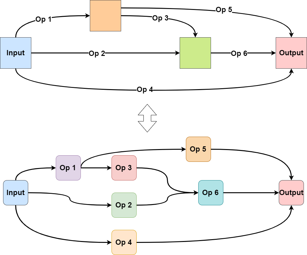
Figure 7: Illustration of how to transform a DARTS-like cell (top) in NAS-Bench-201 to the NAS-Bench-101 format (bottom).

A.4.9 EfficientNet and ProxylessNAS Search Space

For EfficientNet experiment, we take the EfficientNet-B0 network structure as the backbone and define 7 searchable locations, as indicated by the TBS symbol in Table 12. We run GA-NAS to select a type of mobile inverted bottleneck MBConv block. We search for different expansion ratios {1, 3 ,6} and kernel size {3, 5} combinations, which results in 6 candidate MBConv blocks per TBS location.

We conduct 2 GA-NAS searches with different performance estimation methods. In setup 1 we estimate the performance of a candidate network by training it on CIFAR-10 for 20 epochs then compute the test accuracy. In setup 2 we first train a weight-sharing Supernet that has the same structure as the backbone in Table 12, for 500 epochs, and using a ImageNet-224-120 dataset that is subsampled the same way as NAS-Bench-201. The estimated performance in this case is the validation accuracy a candidate network could achieve on ImageNet-224-120 by inheriting weights from the Supernet. For setup 2, training the supernet takes about 20 GPU days on Tesla V100 GPUs, and search takes another GPU day, making a total of 21 GPU days.

Operator	Resolution	#C	#Layers
Conv3x3	$224\times 224$	32	1
TBS	$112\times 112$	16	1
TBS	$112\times 112$	24	2
TBS	$56\times 56$	40	2
TBS	$28\times 28$	80	3
TBS	$14\times 14$	112	3
TBS	$14\times 14$	192	4
TBS	$7\times 7$	320	1
Conv1x1 & Pooling & FC	$7\times 7$	1280	1

Table 12: Macro search backbone network for our EfficientNet experiment. TBS denotes a cell position to be searched, which can be a type of MBConv block. Output denotes a Conv1x1 & Pooling & Fully-connected layer.

Figure 8 presents a visualization on the three single-path networks found by GA-NAS on the EfficientNet search space. Compared to EfficientNet-B0, GA-NAS-ENet-1 significantly reduces the number of trainable weights while maintaining an acceptable accuracy. GA-NAS-ENet-2 improves the accuracy while also reducing the model size. GA-NAS-ENet-3 improves the accuracy further.

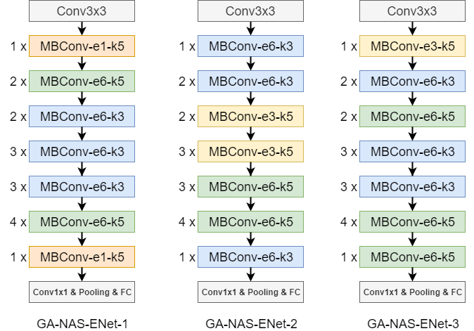
Figure 8: Structures of the single-path networks found by GA-NAS on the EfficientNet search space. In each MBConv block, $e$ denotes expansion ratio and $k$ stands for kernel size.

For ProxylessNAS experiment, we take the ProxylessNAS network structure as the backbone and define 21 searchable locations, as indicated by the TBS symbol in Table 13. We run GA-NAS to search for MBConv blocks with different expansion ratios {3 ,6} and kernel size {3, 5, 7} combinations, which results in 6 candidate MBConv blocks per TBS location.

We train a supernet on ImageNet for 160 epochs (which is the same number of epochs performed by ProxylessNAS weight-sharing search  Cai et al. [2018]) for around 20 GPU days, and conduct an unconstrained search using GA-NAS for around 38 hours on 8 Tesla V100 GPUs in the search space of ProxylessNAS Cai et al. [2018], a major portion out of which, i.e., 29 hours is spent on querying the supernet for architecture performance. Figure 9 presents a visualization of the best architecture found by GA-NAS-ProxylessNAS with better top-1 accuracy and a comparable the number of trainable weights compared to ProxylessNAS-GPU.

Figure 9: Structures of the single-path networks found by GA-NAS on the ProxylessNAS search space.

Operator	Resolution	#C	Identity
Conv3x3	$224\times 224$	32	No
MBConv-e1-k3	$112\times 112$	16	No
TBS	$112\times 112$	24	No
TBS	$56\times 56$	24	Yes
TBS	$56\times 56$	24	Yes
TBS	$56\times 56$	24	Yes
TBS	$56\times 56$	40	No
TBS	$28\times 28$	40	Yes
TBS	$28\times 28$	40	Yes
TBS	$28\times 28$	40	Yes
TBS	$28\times 28$	80	No
TBS	$14\times 14$	80	Yes
TBS	$14\times 14$	80	Yes
TBS	$14\times 14$	80	Yes
TBS	$14\times 14$	96	No
TBS	$14\times 14$	96	Yes
TBS	$14\times 14$	96	Yes
TBS	$14\times 14$	96	Yes
TBS	$14\times 14$	192	No
TBS	$7\times 7$	192	Yes
TBS	$7\times 7$	192	Yes
TBS	$7\times 7$	192	Yes
TBS	$7\times 7$	320	Yes
Avg. Pooling	$7\times 7$	1280	1
FC	$1\times 1$	1000	1

Table 13: Macro search backbone network for our ProxyLessNAS experiment. TBS denotes a cell position to be searched, which can be a type of MBConv block. Identity denotes if an identity shortcut is enabled.

References

- Bender et al. [2020] Gabriel Bender, Hanxiao Liu, Bo Chen, Grace Chu, Shuyang Cheng, Pieter-Jan Kindermans, and Quoc V Le. Can weight sharing outperform random architecture search? an investigation with tunas. In Proceedings of the IEEE/CVF Conference on Computer Vision and Pattern Recognition, pages 14323–14332, 2020.
- Cai et al. [2018] Han Cai, Ligeng Zhu, and Song Han. Proxylessnas: Direct neural architecture search on target task and hardware. arXiv preprint arXiv:1812.00332, 2018.
- Dai et al. [2020] Xiaoliang Dai, Alvin Wan, Peizhao Zhang, Bichen Wu, Zijian He, Zhen Wei, Kan Chen, Yuandong Tian, Matthew Yu, Peter Vajda, et al. Fbnetv3: Joint architecture-recipe search using neural acquisition function. arXiv preprint arXiv:2006.02049, 2020.
- Dong and Yang [2020] Xuanyi Dong and Yi Yang. Nas-bench-201: Extending the scope of reproducible neural architecture search. In International Conference on Learning Representations, 2020.
- Elsken et al. [2018] Thomas Elsken, Jan Hendrik Metzen, and Frank Hutter. Neural architecture search: A survey. arXiv preprint arXiv:1808.05377, 2018.
- Goodfellow et al. [2014] Ian Goodfellow, Jean Pouget-Abadie, Mehdi Mirza, Bing Xu, David Warde-Farley, Sherjil Ozair, Aaron Courville, and Yoshua Bengio. Generative adversarial nets. In Advances in neural information processing systems, pages 2672–2680, 2014.
- Homem-de Mello and Rubinstein [2002] Tito Homem-de Mello and Reuven Y Rubinstein. Rare event estimation for static models via cross-entropy and importance sampling. 2002.
- Jolicoeur-Martineau [2018] Alexia Jolicoeur-Martineau. The relativistic discriminator: a key element missing from standard gan. arXiv preprint arXiv:1807.00734, 2018.
- Kandasamy et al. [2018] Kirthevasan Kandasamy, Willie Neiswanger, Jeff Schneider, Barnabas Poczos, and Eric P Xing. Neural architecture search with bayesian optimisation and optimal transport. In Advances in neural information processing systems, pages 2016–2025, 2018.
- Li and Talwalkar [2020] Liam Li and Ameet Talwalkar. Random search and reproducibility for neural architecture search. In Uncertainty in Artificial Intelligence, pages 367–377. PMLR, 2020.
- Liu et al. [2018] Hanxiao Liu, Karen Simonyan, and Yiming Yang. Darts: Differentiable architecture search. arXiv preprint arXiv:1806.09055, 2018.
- Luo et al. [2020] Renqian Luo, Xu Tan, Rui Wang, Tao Qin, Enhong Chen, and Tie-Yan Liu. Semi-supervised neural architecture search. arXiv preprint arXiv:2002.10389, 2020.
- Morris et al. [2019] Christopher Morris, Martin Ritzert, Matthias Fey, William L Hamilton, Jan Eric Lenssen, Gaurav Rattan, and Martin Grohe. Weisfeiler and leman go neural: Higher-order graph neural networks. In Proceedings of the AAAI Conference on Artificial Intelligence, volume 33, pages 4602–4609, 2019.
- Pham et al. [2018] Hieu Pham, Melody Y Guan, Barret Zoph, Quoc V Le, and Jeff Dean. Efficient neural architecture search via parameter sharing. arXiv preprint arXiv:1802.03268, 2018.