Construction of Diffeomorphisms with Prescribed Jacobian Determinant and Curl

Abstract

The variational principle (VP) is designed to generate non-folding grids (diffeomorphisms) with prescribed Jacobian determinant (JD) and curl. Its solution pool of the original VP is based on an additive formulation and, consequently, is not invariant in the diffeomorphic Lie algebra. The original VP works well when the prescribed pair of JD and curl is calculated from a diffeomorphism, but not necessarily when the prescribed JD and curl are not known to come from a diffeomorphism. This issue is referred as the mismatched pair problem. In spite of that, the original VP works effectively in 2D grid generations. To resolve these issues, in this paper, we describe a new version of VP (revised VP), which is based on composition of transformations and, therefore, is invariant in the Lie algebra. The revised VP seems have overcome the inaccuracy of original VP in 3D grid generations. In the following sections, the mathematical derivations are presented. It is shown that the revised VP can calculate the inverse transformation of a known diffeomorphism. Its inverse consistency and transitivity of transformations are also demonstrated numerically. Moreover, a computational strategy is formulated based on the new version of VP to handle the mismatch issue and is demonstrated with preliminary result.

1 Introduction

Computational construction of diffeomorphism is an active research field in computational geometry. For instance, conformal differential geometry [Gu] led by Gu achieved remarkable success in surface differential geometry. Whereas, the aims of this study is about how to characterize and control a meaningful distribution of grid points over a volumetric domain, such as in [Grajewski, Liseikin]. This is the problem of adaptive generation of non-folding grids. One approach to the task is to find a differentiable and invertible transformation, i.e., a diffeomorphism, $\boldsymbol{T}$ by controlling its JD which models local cell-size, such as in [Brackbill, DacMos, Moser, Huang]. Its idea has been widely transfered and applied in constructing deformable image registration methods, such as in [ChenY, Lee, Joshi, Joshi2, Sotiras]. A grid generation method in [Cai], the deformation constructs $\boldsymbol{T}$ with prescribed JD, by a scalar $0<f\in C^{1}$, whose key component is the solution to a $\bf{divergence-curl}$ system (similar to the constraints of (2)). Its divergence is approximated by $f-1$ and curl is assigned by $\boldsymbol{0}$, due to the challenge of realizing curl before hand. Consequently, grids generated by the deformation method is not unique due to the lack of curl information, in [Liao], which models the local cell-rotation. To overcome this problem, the original VP was proposed in [ChenXi] and studied further in [Zhou]. In 3D grid generations, the original VP only provides inaccurate approximations around the true solution. The authors attempted to analyze the uniqueness of such transformations, but it turned out cannot be completed for the reason that JD of a transformation is merely an approximation to the divergence of the transformation. Fortunately, this does not undermine VP to produce well approximated grids and in turn allows mismatched values of prescribed JD and curl under certain range.

However, a novel image atlas construction method proposed in [Zhou] utilizes the original VP and requires it (i) to accept wider ranges of mismatched JD and curl and (ii) to optimize JD and curl in a separable manner so one may investigate how each of them affect a diffeomorphism. Another limitation of the original VP is its consideration of small deformations $\boldsymbol{T}=\boldsymbol{id}+\boldsymbol{u}\in H^{2}_{0}(\mathrm{\Omega})$ where $\boldsymbol{u}$ is the displacement field and $\boldsymbol{id}$ is the identity map (uniform grid), such as in [Joshi], whose function composition “$\circ$” is approximated by $\boldsymbol{T}_{2}\circ\boldsymbol{T}_{1}\approx\boldsymbol{T}_{1}+\boldsymbol{u}_{2}=\boldsymbol{id}+\boldsymbol{u}_{1}+\boldsymbol{u}_{2}=\boldsymbol{id}+\boldsymbol{u}_{2}+\boldsymbol{u}_{1}=\boldsymbol{T}_{2}+\boldsymbol{u}_{1}\approx\boldsymbol{T}_{1}\circ\boldsymbol{T}_{2}$. From a computational perspective, it risks having function composition maps outside of the collection $\boldsymbol{T}\in H^{2}_{0}(\mathrm{\Omega})$ that forms a diffeomorphism group [Bauer, Joshi2]. Therefore, in this paper, to resolve (i), (ii) and to broaden the transformations that VP can characterize, we fundamentally revise VP to consider transformations taking composition as the left-translation. Surprisingly, this revision also overcome the inaccuracy of the original VP in 3D grid generation.

The structure of the paper is organized as follow. In section 2, we reformulated VP to cope with composition as left-translation. In section 3, examples are provided to demonstrate the effectiveness of the revised VP; In section LABEL:demo2, a computational strategy is proposed to handle the mismatch issue. The numerical experiments run with MatLab codes on a desktop PC with ADM Ryzen-9 12-core Processor, 16 GB RAM and NVIDA GeForce RTX 3080 GPU.

2 New Version of Variational Principle

Let a simply-connected, bounded $\mathrm{\Omega}\subset\mathbb{R}^{3}$ (similar in $\mathbb{R}^{2}$) be the domain and $\boldsymbol{x}=(x,y,z)\in\mathrm{\Omega}$. Let a scalar function $f_{o}>0$ and a vector-valued function $\boldsymbol{g}_{o}$ on $\mathrm{\Omega}$ satisfy $\int_{\mathrm{\Omega}}f_{o}(\boldsymbol{x})d\boldsymbol{x}=|\mathrm{\Omega}|$ and $\nabla\cdot\boldsymbol{g}_{o}=0$, respectively. Given $\boldsymbol{\phi}_{o}\in H^{2}_{0}(\mathrm{\Omega})$, we look for a diffeomorphic transformation $\boldsymbol{\phi}=\boldsymbol{\phi}_{\boldsymbol{m}}\circ\boldsymbol{\phi}_{o}=\boldsymbol{\phi}_{\boldsymbol{m}}(\boldsymbol{\phi}_{o})\in H^{2}_{0}(\mathrm{\Omega})$, where $\boldsymbol{\phi}_{\boldsymbol{m}}=\boldsymbol{id}+\boldsymbol{u}$ is an intermediate transformation that left-translates $\boldsymbol{\phi}_{o}$ to $\boldsymbol{\phi}$ and implies $\delta\boldsymbol{\phi}_{\boldsymbol{m}}=\delta\boldsymbol{u}$, that the cost functional — sum of squared differences ($SSD$) is minimized:

$$SSD(\boldsymbol{\phi})=\frac{1}{2}\int_{\mathrm{\Omega}}[(\text{det}\nabla\boldsymbol{\phi}-f_{o})^{2}+|\nabla\times\boldsymbol{\phi}-\boldsymbol{g}_{o}|^{2}]d\boldsymbol{x}$$ (1)

$$\text{ subjects to }\left\{\begin{aligned} &\begin{aligned} \nabla\cdot\boldsymbol{u}&=f-1\\ \nabla\times\boldsymbol{u}&=\boldsymbol{g}\end{aligned}\end{aligned}\right.\Rightarrow\mathrm{\Delta}\boldsymbol{u}=\nabla f-\nabla\times\boldsymbol{g}=\boldsymbol{F}\text{ in }\mathrm{\Omega},$$ (2)

with $\boldsymbol{u}=\boldsymbol{0}$ on $\partial\mathrm{\Omega}$ where $f$, $\boldsymbol{g}$ and $\boldsymbol{F}$ are control functions. Its variational gradient with respect to the control function $\boldsymbol{F}$ can be derive as follows. Denote $P=\text{det}\nabla\boldsymbol{\phi}-f_{o}$ and $\boldsymbol{Q}=\nabla\times\boldsymbol{\phi}-\boldsymbol{g}_{o}$, then, for all $\delta\boldsymbol{F}$ vanishing on $\partial\mathrm{\Omega}$,

$$\delta SSD(\boldsymbol{\phi}_{\boldsymbol{m}} \circ\boldsymbol{\phi}_{o})=\int_{\mathrm{\Omega}}[(\text{det}\nabla\boldsymbol{\phi}-f_{o})\delta\text{det}\nabla(\boldsymbol{\phi}_{\boldsymbol{m}}\circ\boldsymbol{\phi}_{o})+(\nabla\times\boldsymbol{\phi}-\boldsymbol{g}_{o})\cdot\delta\nabla\times(\boldsymbol{\phi}_{\boldsymbol{m}}\circ\boldsymbol{\phi}_{o})]d\boldsymbol{x}$$

$$= \int_{\mathrm{\Omega}}[P\delta\text{det}\nabla\boldsymbol{\phi}_{\boldsymbol{m}}\text{det}\nabla\boldsymbol{\phi}_{o}+\boldsymbol{Q}\cdot\delta\begin{pmatrix}\nabla\phi_{\boldsymbol{m}3}\cdot(\boldsymbol{\phi}_{o})_{y}-\nabla\phi_{\boldsymbol{m}2}\cdot(\boldsymbol{\phi}_{o})_{z}\\ -\nabla\phi_{\boldsymbol{m}3}\cdot(\boldsymbol{\phi}_{o})_{x}+\nabla\phi_{\boldsymbol{m}1}\cdot(\boldsymbol{\phi}_{o})_{z}\\ \nabla\phi_{\boldsymbol{m}2}\cdot(\boldsymbol{\phi}_{o})_{x}-\nabla\phi_{\boldsymbol{m}1}\cdot(\boldsymbol{\phi}_{o})_{y}\end{pmatrix}]d\boldsymbol{x}$$

$$=\int_{\mathrm{\Omega}}[P \text{det}\nabla\boldsymbol{\phi}_{o}(\delta u_{1x}\phi_{\boldsymbol{m}2y}\phi_{\boldsymbol{m}3z}+\phi_{\boldsymbol{m}1x}\delta u_{2y}\phi_{\boldsymbol{m}3z}+\phi_{\boldsymbol{m}1x}\phi_{\boldsymbol{m}2y}\delta u_{3z}-\delta u_{1x}\phi_{\boldsymbol{m}2z}\phi_{\boldsymbol{m}3y}$$

$$-\phi_{\boldsymbol{m}1x} \delta u_{2z}\phi_{\boldsymbol{m}3y}-\phi_{\boldsymbol{m}1x}\phi_{\boldsymbol{m}2z}\delta u_{3y}-\delta u_{1y}\phi_{\boldsymbol{m}3z}\phi_{\boldsymbol{m}2x}-\phi_{\boldsymbol{m}1y}\delta u_{3z}\phi_{\boldsymbol{m}2x}-\phi_{\boldsymbol{m}1y}\phi_{\boldsymbol{m}3z}\delta u_{2x}$$

$$+\delta u_{1y} \phi_{\boldsymbol{m}3x}\phi_{\boldsymbol{m}2z}+\phi_{\boldsymbol{m}1y}\delta u_{3x}\phi_{\boldsymbol{m}2z}+\phi_{\boldsymbol{m}1y}\phi_{\boldsymbol{m}3x}\delta u_{2z}+\delta u_{1z}\phi_{\boldsymbol{m}2x}\phi_{\boldsymbol{m}3y}+\phi_{\boldsymbol{m}1z}\delta u_{2x}\phi_{\boldsymbol{m}3y}$$

$$+\phi_{\boldsymbol{m}1z} \phi_{\boldsymbol{m}2x}\delta u_{3y}-\delta u_{1z}\phi_{\boldsymbol{m}2y}\phi_{\boldsymbol{m}3x}-\phi_{\boldsymbol{m}1z}\delta u_{2y}\phi_{\boldsymbol{m}3x}-\phi_{\boldsymbol{m}1z}\phi_{\boldsymbol{m}2y}\delta u_{3x})$$

$$+\begin{pmatrix}Q_{1}\\ Q_{2}\\ Q_{3}\end{pmatrix} \cdot\begin{pmatrix}\delta u_{3x}\phi_{o1y}+\delta u_{3y}\phi_{o2y}+\delta u_{3z}\phi_{o3y}-\delta u_{2x}\phi_{o1z}-\delta u_{2y}\phi_{o2z}-\delta u_{2z}\phi_{o3z}\\ -\delta u_{3x}\phi_{o1x}-\delta u_{3y}\phi_{o2x}-\delta u_{3z}\phi_{o3x}+\delta u_{1x}\phi_{o1z}+\delta u_{1y}\phi_{o2z}+\delta u_{1z}\phi_{o3z}\\ \delta u_{2x}\phi_{o1x}+\delta u_{2y}\phi_{o2x}+\delta u_{2z}\phi_{o3x}-\delta u_{1x}\phi_{o1y}-\delta u_{1y}\phi_{o2y}-\delta u_{1z}\phi_{o3y}\end{pmatrix}]d\boldsymbol{x}$$

$$=\int_{\mathrm{\Omega}}[(P \text{det}\nabla\boldsymbol{\phi}_{o}\begin{pmatrix}\phi_{\boldsymbol{m}2y}\phi_{\boldsymbol{m}3z}-\phi_{\boldsymbol{m}3y}\phi_{\boldsymbol{m}2z}\\ \phi_{\boldsymbol{m}3x}\phi_{\boldsymbol{m}2z}-\phi_{\boldsymbol{m}2x}\phi_{\boldsymbol{m}3z}\\ \phi_{\boldsymbol{m}2x}\phi_{\boldsymbol{m}3y}-\phi_{\boldsymbol{m}2y}\phi_{\boldsymbol{m}3x}\end{pmatrix}+\begin{pmatrix}Q_{2}\phi_{o1z}-Q_{3}\phi_{o1y}\\ Q_{2}\phi_{o2z}-Q_{3}\phi_{o2y}\\ Q_{2}\phi_{o3z}-Q_{3}\phi_{o3y}\end{pmatrix})\cdot\nabla\delta u_{1}$$

$$+ (P\text{det}\nabla\boldsymbol{\phi}_{o}\begin{pmatrix}\phi_{\boldsymbol{m}3y}\phi_{\boldsymbol{m}1z}-\phi_{\boldsymbol{m}1y}\phi_{\boldsymbol{m}3z}\\ \phi_{\boldsymbol{m}1x}\phi_{\boldsymbol{m}3z}-\phi_{\boldsymbol{m}1z}\phi_{\boldsymbol{m}3x}\\ \phi_{\boldsymbol{m}3x}\phi_{\boldsymbol{m}1y}-\phi_{\boldsymbol{m}1x}\phi_{\boldsymbol{m}3y}\end{pmatrix}+\begin{pmatrix}-Q_{1}\phi_{o1z}+Q_{3}\phi_{o1x}\\ -Q_{1}\phi_{o2z}+Q_{3}\phi_{o2x}\\ -Q_{1}\phi_{o3z}+Q_{3}\phi_{o3x}\end{pmatrix})\cdot\nabla\delta u_{2}$$

$$+ (P\text{det}\nabla\boldsymbol{\phi}_{o}\begin{pmatrix}\phi_{\boldsymbol{m}1y}\phi_{\boldsymbol{m}2z}-\phi_{\boldsymbol{m}2y}\phi_{\boldsymbol{m}1z}\\ \phi_{\boldsymbol{m}2x}\phi_{\boldsymbol{m}1z}-\phi_{\boldsymbol{m}1x}\phi_{\boldsymbol{m}2z}\\ \phi_{\boldsymbol{m}1x}\phi_{\boldsymbol{m}2y}-\phi_{\boldsymbol{m}2x}\phi_{\boldsymbol{m}1y}\end{pmatrix}+\begin{pmatrix}Q_{1}\phi_{o1y}-Q_{2}\phi_{o1x}\\ Q_{1}\phi_{o2y}-Q_{2}\phi_{o2x}\\ Q_{1}\phi_{o3y}-Q_{2}\phi_{o3x}\end{pmatrix})\cdot\nabla\delta u_{3}]d\boldsymbol{x}$$

$$= \int_{\mathrm{\Omega}}(\boldsymbol{A}_{1}\cdot\nabla\delta u_{1}+\boldsymbol{A}_{2}\cdot\nabla\delta u_{2}+\boldsymbol{A}_{3}\cdot\nabla\delta u_{3})d\boldsymbol{x}.$$

Here, the “big vector”s are now denoted as $\boldsymbol{A}_{i}$, where $i=1,2,3$. By $Green$’s identities with fixed boundary condition and for some $B_{i}$ such that $\mathrm{\Delta}B_{i}=-\nabla\cdot\boldsymbol{A}_{i}$ and $i=1,2,3$, then it can be carried to,

$$\delta SSD= \int_{\mathrm{\Omega}}(-\nabla\cdot\boldsymbol{A}_{1}\delta u_{1}-\nabla\cdot\boldsymbol{A}_{2}\delta u_{2}-\nabla\cdot\boldsymbol{A}_{3}\delta u_{3})d\boldsymbol{x}$$ (3)

$$= \int_{\mathrm{\Omega}}(\mathrm{\Delta}B_{1}\delta u_{1}+\mathrm{\Delta}B_{2}\delta u_{2}+\mathrm{\Delta}B_{3}\delta u_{3})d\boldsymbol{x}$$

$$= \int_{\mathrm{\Omega}}(B_{1}\delta\mathrm{\Delta}u_{1}+B_{2}\delta\mathrm{\Delta}u_{2}+B_{3}\delta\mathrm{\Delta}u_{3})d\boldsymbol{x}$$

$$= \int_{\mathrm{\Omega}}(\boldsymbol{B}\cdot\delta\mathrm{\Delta}\boldsymbol{u})d\boldsymbol{x}$$

$$= \int_{\mathrm{\Omega}}(\boldsymbol{B}\cdot\delta\boldsymbol{F})d\boldsymbol{x}\qquad\Rightarrow\qquad\frac{\partial SSD}{\partial\boldsymbol{F}}=\boldsymbol{B}.$$

To give a more completed view, the variational gradients of $SSD$ with respect to $f$ and $\boldsymbol{g}$ are included as well. For arbitrary $\delta f$ and $\delta\boldsymbol{g}$, one may get $\delta\mathrm{\Delta}\boldsymbol{u}=\nabla\delta f-\nabla\times\delta\boldsymbol{g}$, then, from (3), it can be derived,

$$\delta SSD= \int_{\mathrm{\Omega}}\boldsymbol{B}\cdot(\nabla\delta f-\nabla\times\delta\boldsymbol{g})d\boldsymbol{x}$$

$$= \int_{\mathrm{\Omega}}[\boldsymbol{B}\cdot\nabla\delta f-B_{1}(\delta g_{3y}+\delta g_{2z})+B_{2}(\delta g_{3x}-\delta g_{1z})-B_{3}(\delta g_{2x}+\delta g_{1y})]d\boldsymbol{x}$$

$$= \int_{\mathrm{\Omega}}[\boldsymbol{B}\cdot\nabla\delta f+\begin{pmatrix}0\\ B_{3}\\ -B_{2}\end{pmatrix}\cdot\nabla\delta g_{1}+\begin{pmatrix}-B_{3}\\ 0\\ B_{1}\end{pmatrix}\cdot\nabla\delta g_{2}+\begin{pmatrix}B_{2}\\ -B_{1}\\ 0\end{pmatrix}\cdot\nabla\delta g_{3}]d\boldsymbol{x}$$

$$= \int_{\mathrm{\Omega}}[-\nabla\cdot\boldsymbol{b}\delta f-\begin{pmatrix}B_{3y}-B_{2z}\\ -B_{3x}+B_{1z}\\ B_{2x}-B_{1y}\end{pmatrix}\cdot\delta\boldsymbol{g}]d\boldsymbol{x}$$

$$= \int_{\mathrm{\Omega}}-\nabla\cdot\boldsymbol{B}\delta fd\boldsymbol{x}+\int_{\mathrm{\Omega}}-\nabla\times\boldsymbol{B}\cdot\delta\boldsymbol{g}d\boldsymbol{x}$$

$$\Rightarrow\quad\frac{\partial SSD}{\partial f}=-\nabla\cdot\boldsymbol{B}\quad\text{ and }\quad\frac{\partial SSD}{\partial\boldsymbol{g}}=-\nabla\times\boldsymbol{B}.$$ (4)

A gradient descent based algorithm is provided below. $\triangle t$ is the step-size of gradients. Major computational costs occur in solving $Poisson$ equations by a Fast Fourier Transform $Poisson$ solver, denoted as FFT. Define $ratio=SSD_{final}/SSD_{initial}$ and let $\boldsymbol{F}_{k}$ be the control functions to be optimized.

Algorithm 1 $[\boldsymbol{\phi}_{k},\boldsymbol{\phi}^{k}_{\boldsymbol{m}}]=$ revisedVP($f_{o}$, $\boldsymbol{g}_{o}$, $\boldsymbol{\phi}_{o}$)

 

• 1: set $\triangle t$, $t_{tol}$, $ratio$, $ratio_{tol}$, $k_{max}$, $t_{up}$, $t_{down}$, $better=1$, $k=0$;

• 2: initialize $\boldsymbol{F}_{k}=\boldsymbol{0}$ ($=1$ when optimize along JD direction of (4)), $\boldsymbol{b}_{k}=\boldsymbol{0}$, $\boldsymbol{\phi}_{k}=\boldsymbol{\phi}_{o}$;

• 3: while $\triangle t>t_{tol}$ and $ratio>ratio_{tol}$ and $k<k_{max}$;

  • 4: if $better=1$

    • 5: $k=k+1$

    • 6: solve for $\boldsymbol{B}_{k}$ from $\mathrm{\Delta}B_{i}=-\nabla\cdot\boldsymbol{A}_{i}$ by FFT where $i=1,2,3$;

  • 7: update $\boldsymbol{F}_{k}=\boldsymbol{F}_{k-1}-\triangle t*\boldsymbol{b}_{k}$;

  • 8: solve for $\boldsymbol{u}_{k}$ from $\mathrm{\Delta}\boldsymbol{u}_{k}=\boldsymbol{F}_{k}$ by FFT

  • 9: update $\boldsymbol{\phi}_{k}=\boldsymbol{\phi}^{k}_{\boldsymbol{m}}(\boldsymbol{\phi}_{o})$ by interpolation, where $\boldsymbol{\phi}^{k}_{\boldsymbol{m}}=\boldsymbol{id}+\boldsymbol{u}_{k}$;

  • 10: compute $SSD$ and $ratio$;

  • 11: if $SSD$ decrease,

    • 12: $better=1$

    • 13: $\triangle t=\triangle t*t_{up}$;

    • 14: $\boldsymbol{F}_{k-1}=\boldsymbol{F}_{k}$;

    else

    • 15: $better=0$

    • 16: $\triangle t=\triangle t*t_{down}$.

3 Numerical Examples of Revised VP

E.g.3.1 is an example of a 3D grid reconstruction by the revised VP which demonstrates this work can be applied in 3D scenario. For more intuitive and clear visualizations, the rest of the examples are provided in 2D only. E.g.3.2 shows the revised VP is capable of constructing inverse transformation; E.g.3.3 and LABEL:eg3 confirm that the computational solutions of the revised VP satisfy inverse consistency and transitivity, which are expected in a diffeomorphism group. In all figures, “a” vs “b” means coloured in red “a” superposes on coloured in black “b”, except for displacement fields comparison of E.g.3.1, which “c” vs “d” means coloured in blue “c” superposes on coloured in green “d”.

3.1 $\mathbf{Example}$: 3D Grid Reconstruction Comparison between the Original and Revised VPs

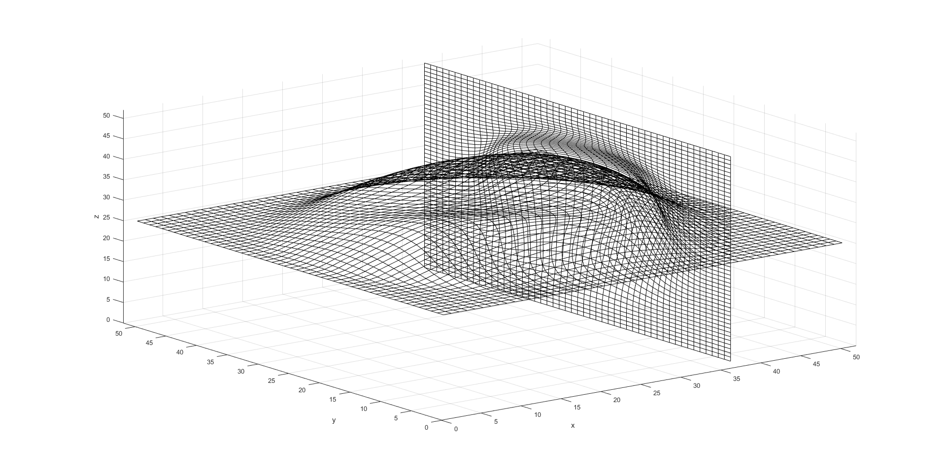
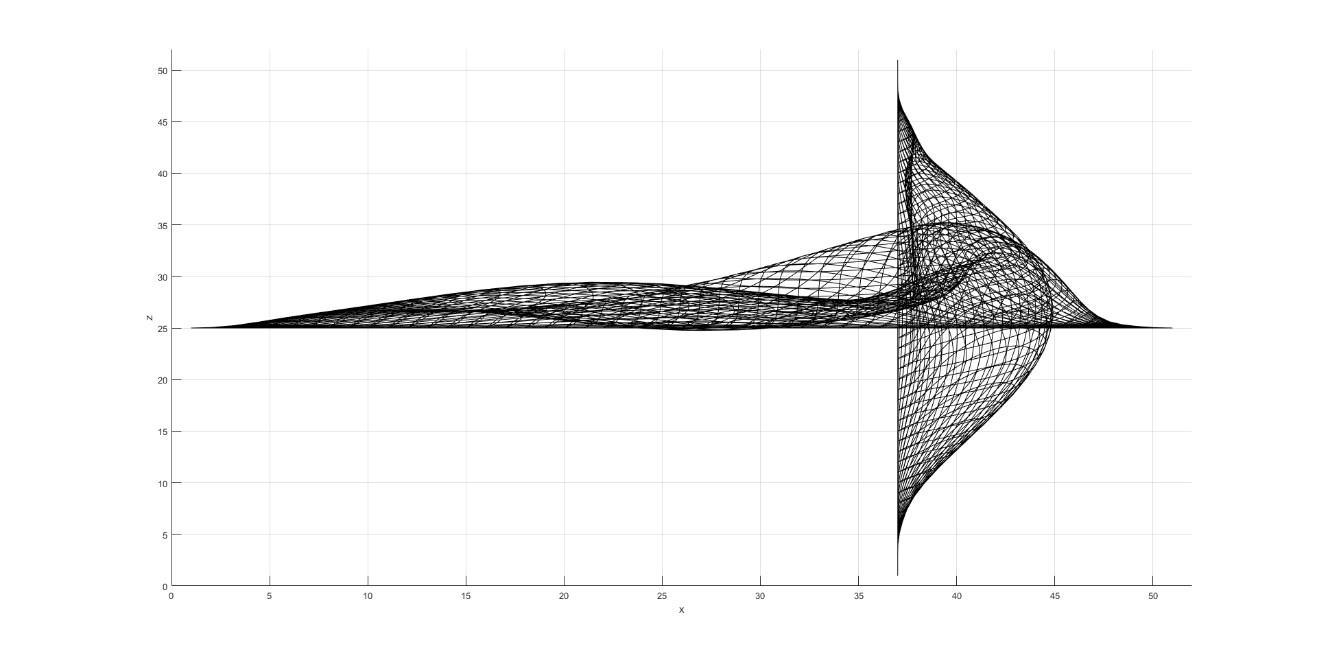
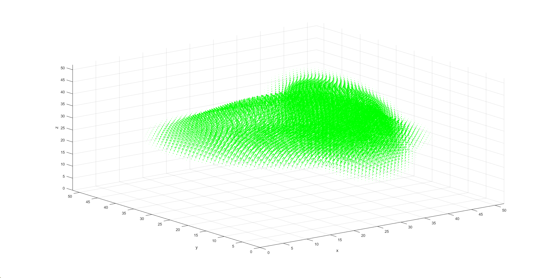
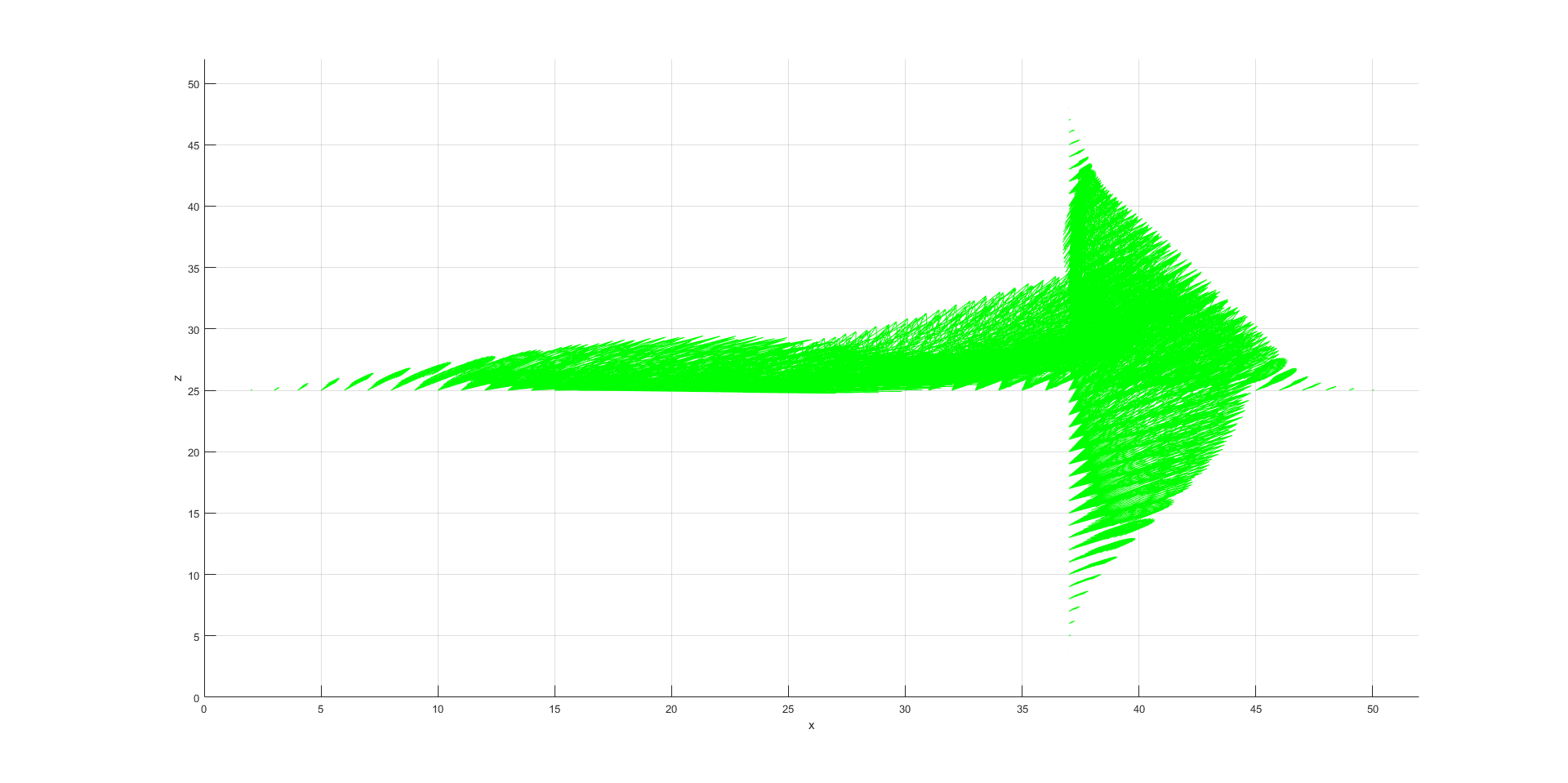
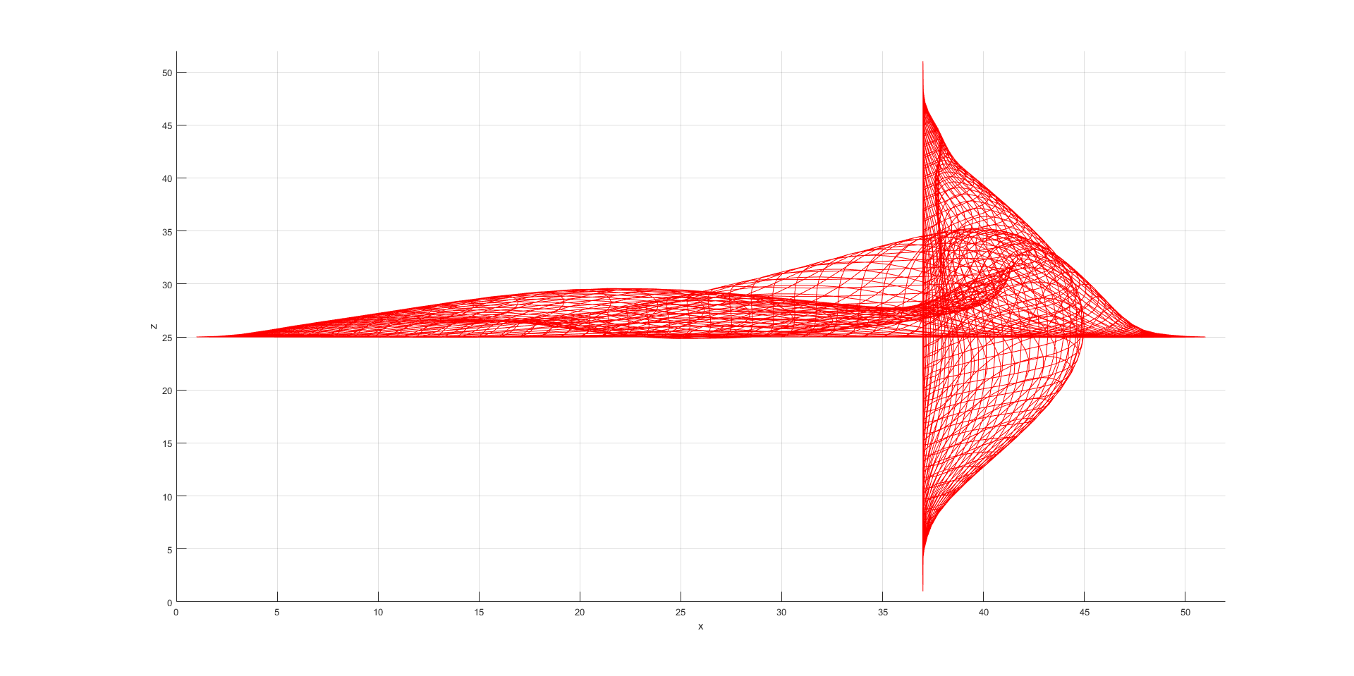
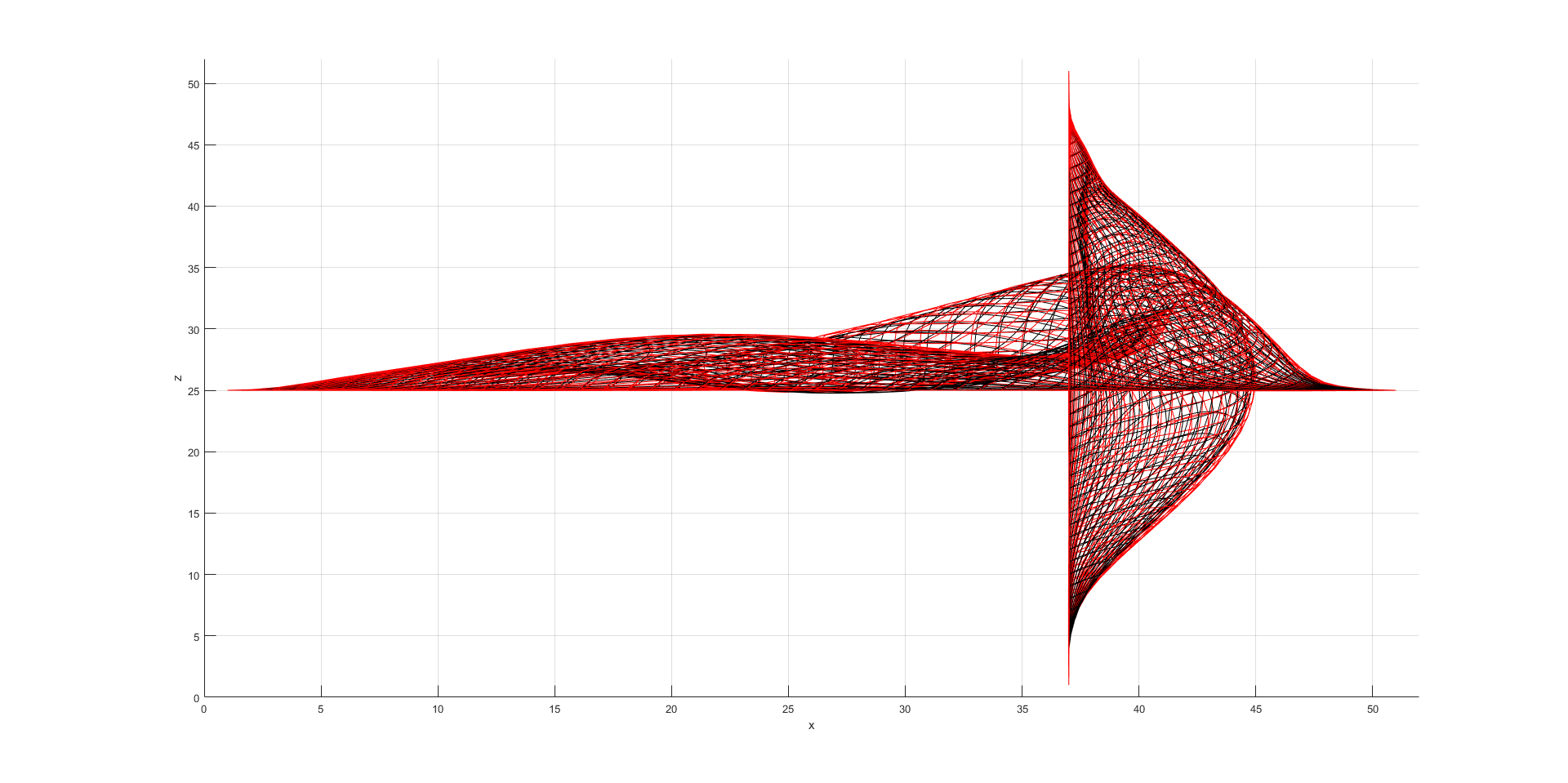
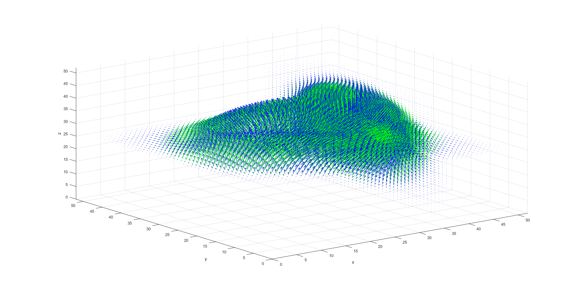
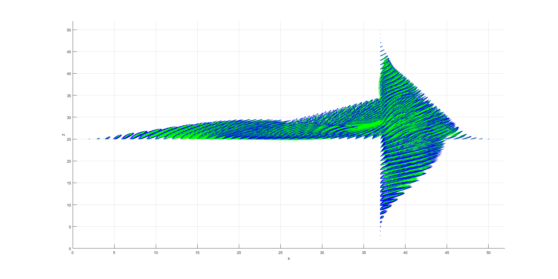
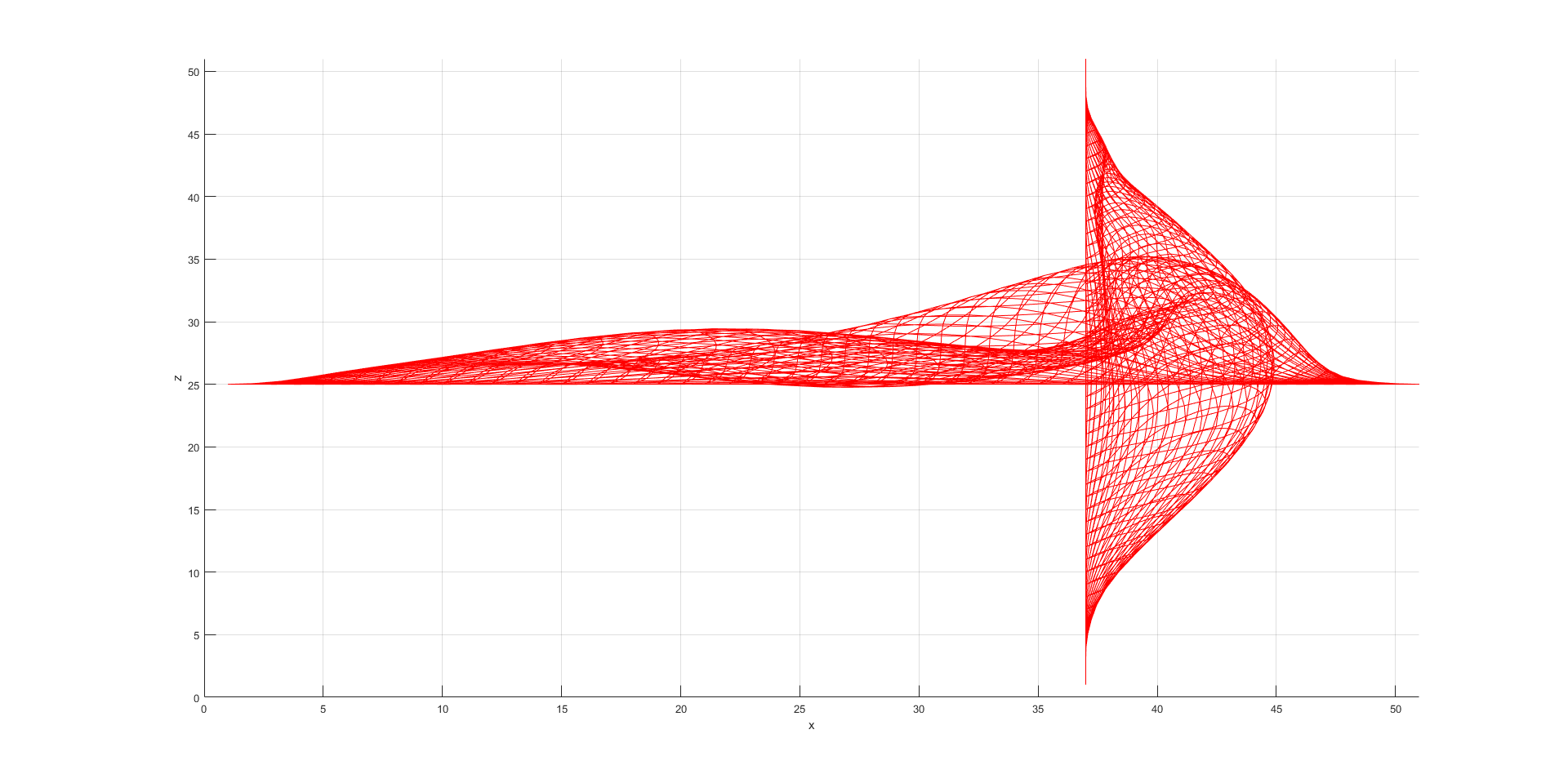
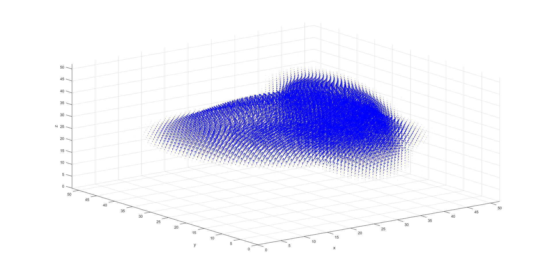
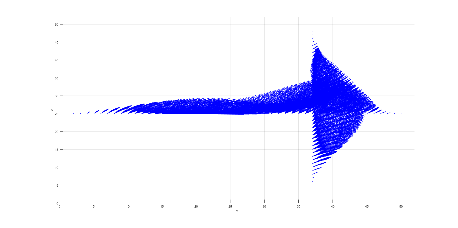
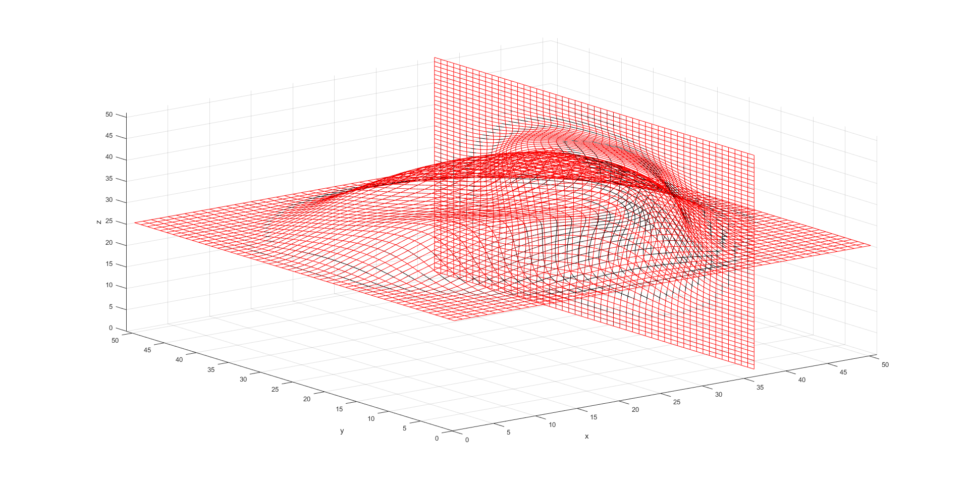
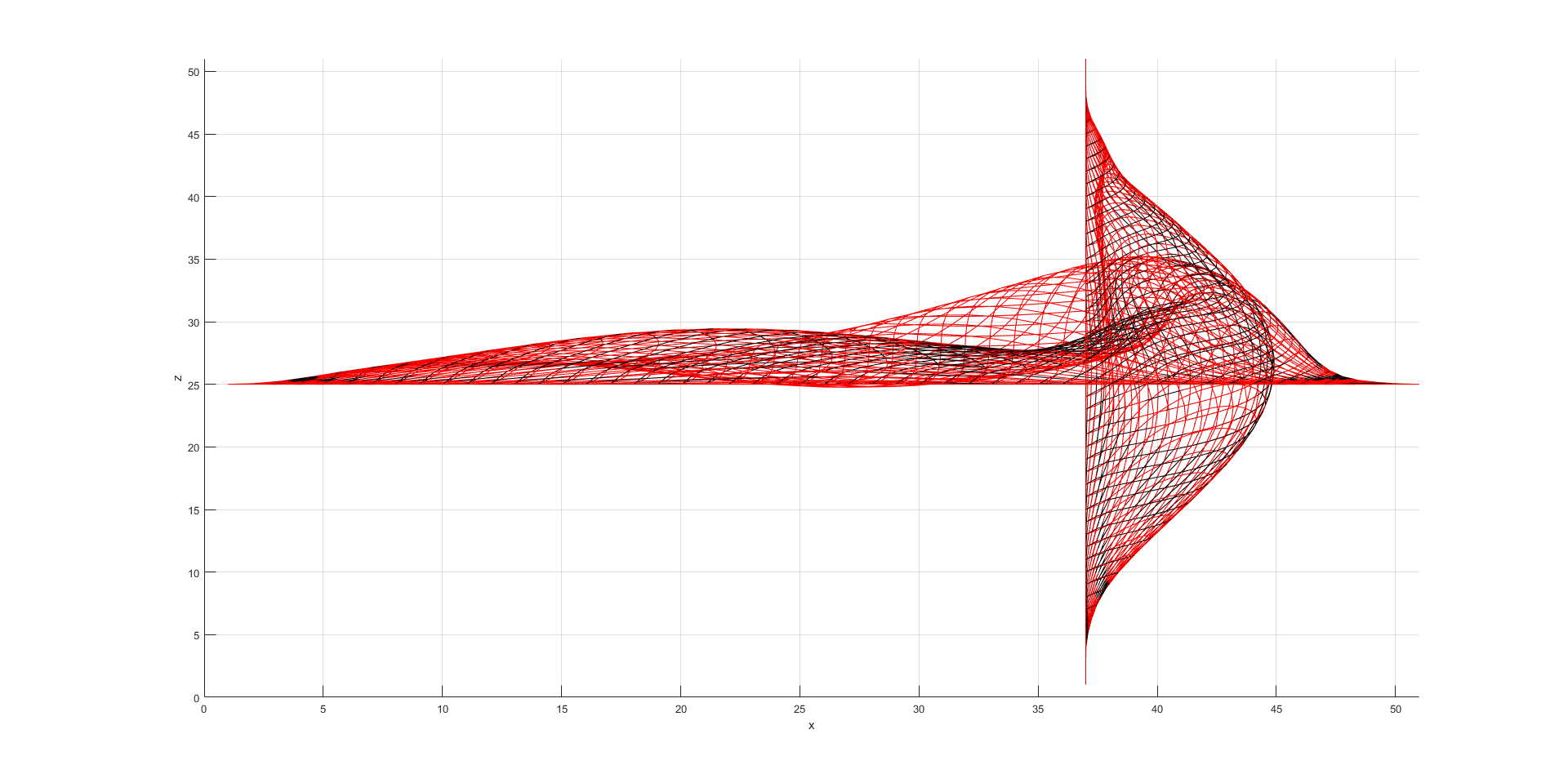
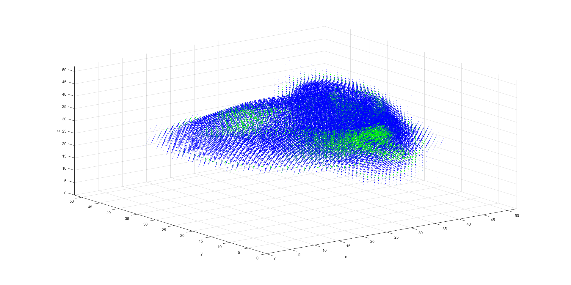
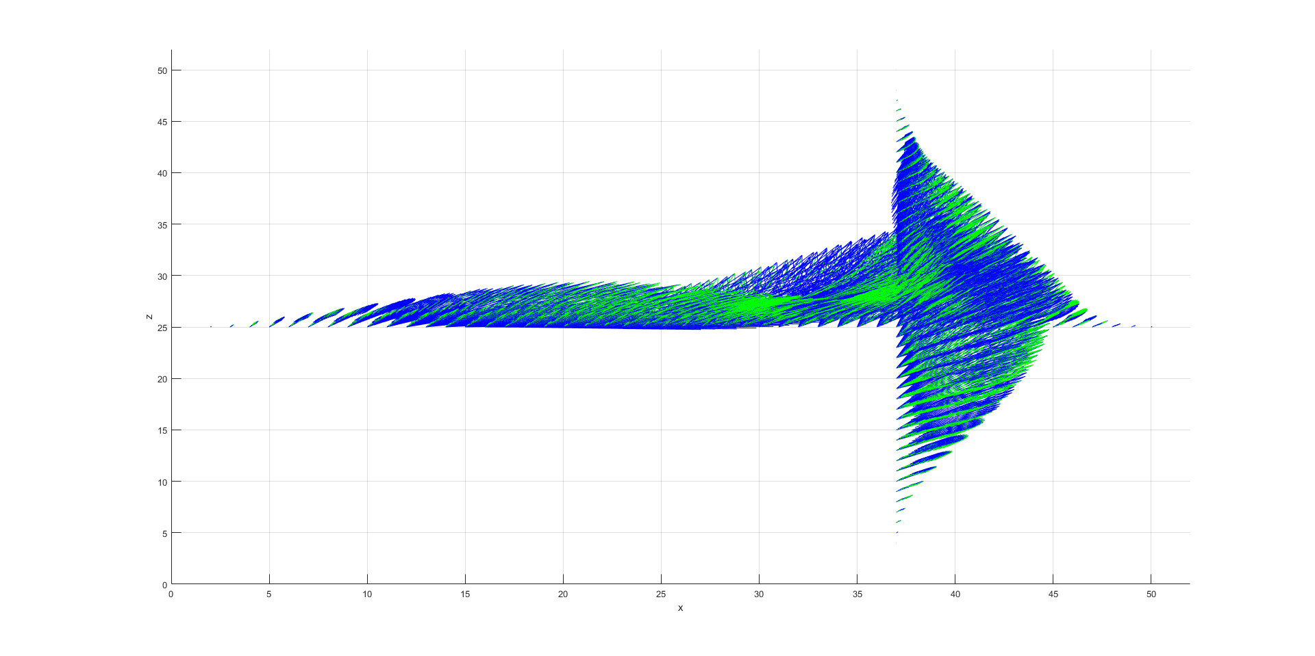
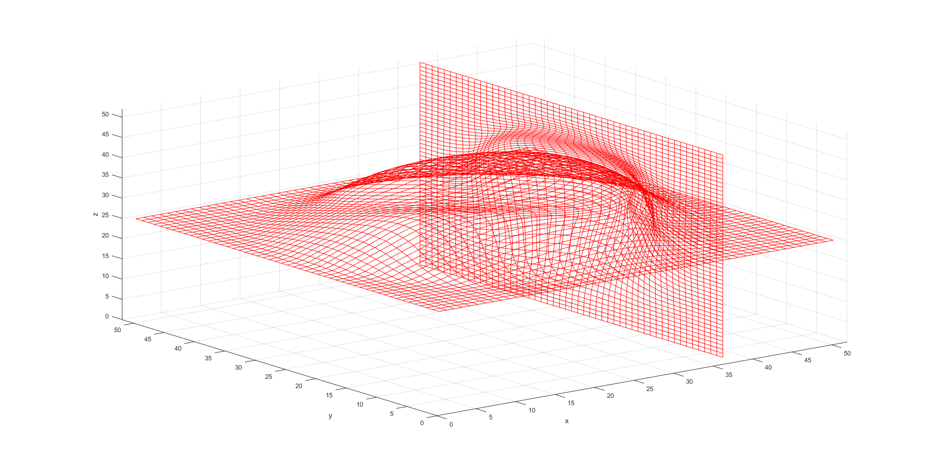
This example demonstrate revised VP achieves better solutions over the original VP proposed in [ChenXi]. Given a 3D grid in black $\boldsymbol{\Phi}$ and its displacement vector field $\boldsymbol{U}=\boldsymbol{\Phi}-\boldsymbol{id}$ in green, in Fig.1, $\boldsymbol{\Phi}$ is manually built by multiple times of applying cutoff rotation and displacement over the domain $\mathrm{\Omega}=[1,51]^{3}$ such that det$\nabla\boldsymbol{\Phi}>0.1734$, i.e., $\boldsymbol{\Phi}$ has non-folding grids. For a cleaner visualization, all 3D grids and their displacement fields are only plotted on the 25-th frame along $z$-axis and the 37-th frame along $x$-axis. Define $f_{o}=$det$\nabla\boldsymbol{\Phi}$ and $\boldsymbol{g}_{o}=\nabla\times\boldsymbol{\Phi}$ as the prescribed JD and curl.

(a) $\boldsymbol{\Phi}$

(b) $\boldsymbol{\Phi}$ ($xz$-plain)

(c) $\boldsymbol{U}$

(d) $\boldsymbol{U}$ ($xz$-plain)

Figure 1: Given ground truth (GT)

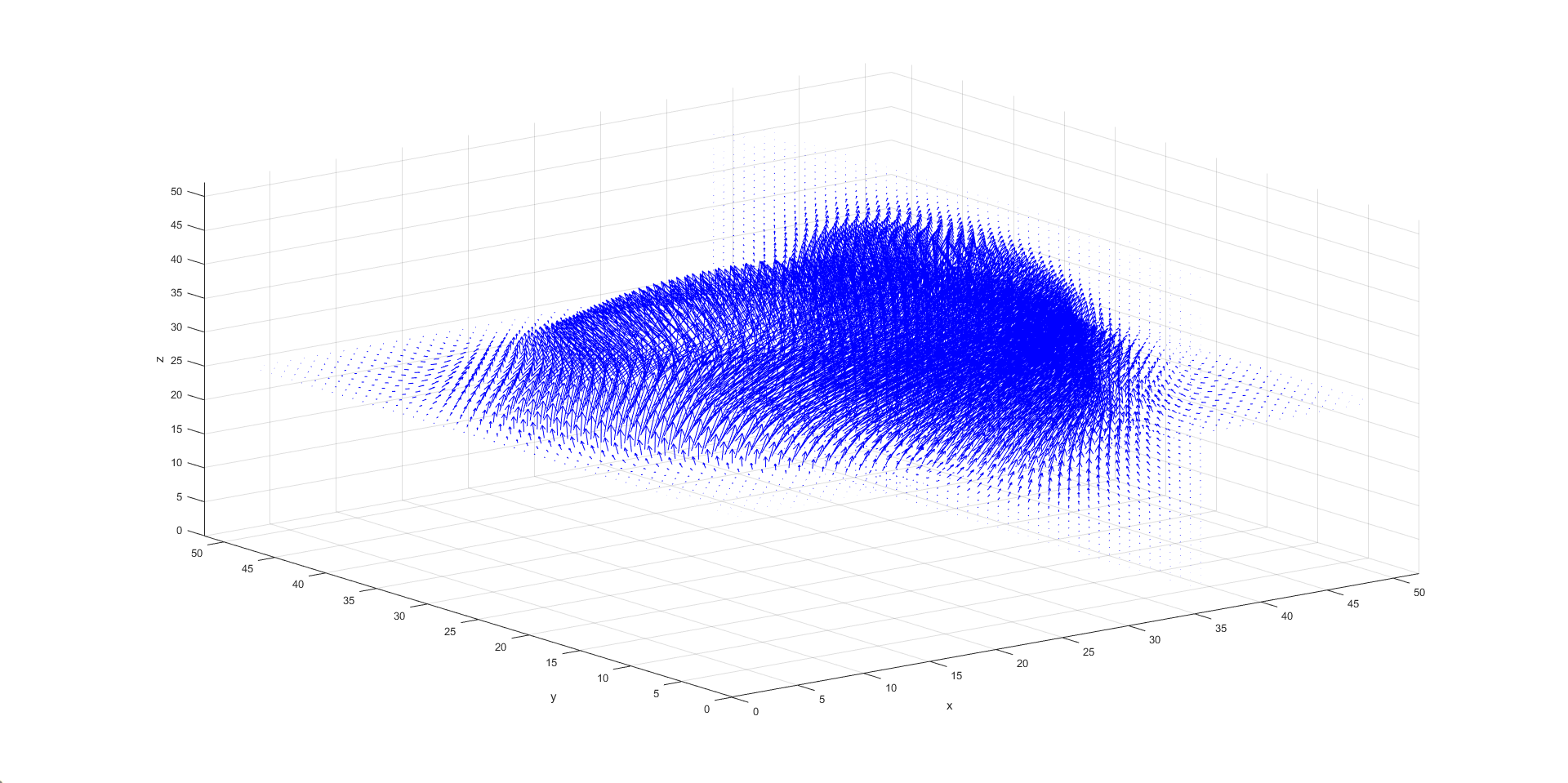
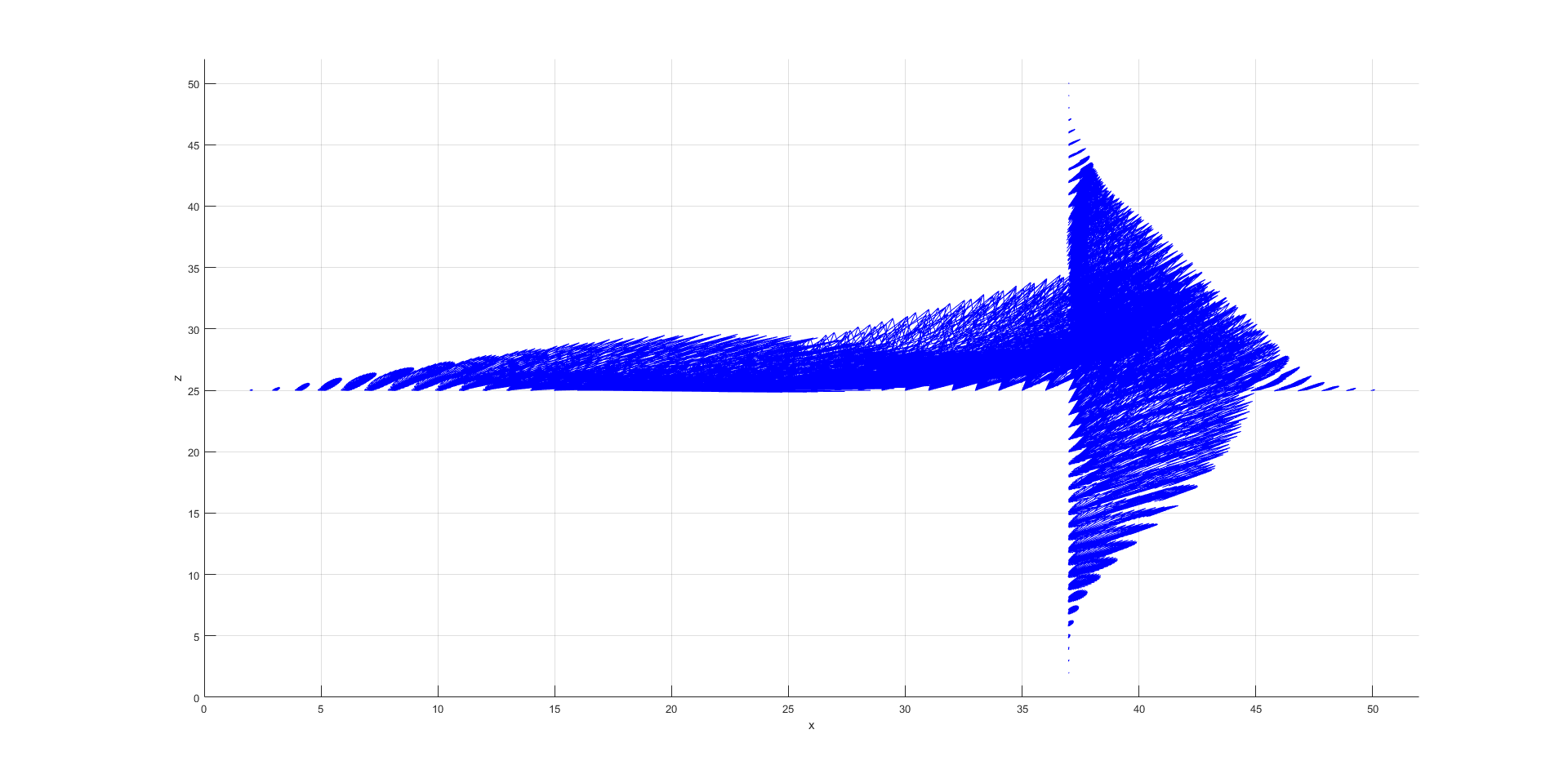
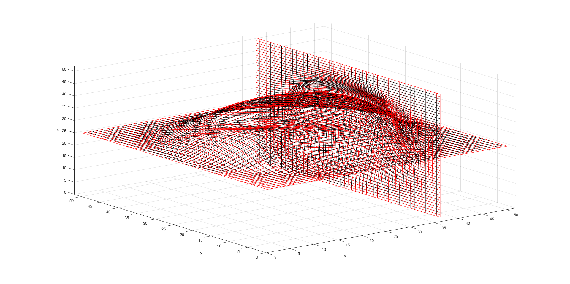
Fig.2(a-d) is the solution of original VP and is superposed on the GT in Fig.2(e-h). It can be visually seen that red grid lines of the solution by original VP do not line-up well with GT in black grid, in Fig.2(e), i.e., a better solution would have covered more black grid. The displacement vector field of original VP, in blue, is not pointing so close to the directions where the displacement vector field of GT points to, in Fig.2(h). Comparing to the solution of revised VP, in Fig.3(a-d), that also is superposed on GT, in Fig.3(e-h), and there is only a small portion of the black grid and the green vectors stay uncovered by the solution of revised VP, which means revised VP provides much better solutions over the original VP. This observation is confirmed by measurements in the following Table.1. It also recorded the revised VP had reached the $ratio$-tolerance, $10^{-4}$%, within lesser iterations and computational time.

(a) $\boldsymbol{\Phi}_{ovp}$

(b) $\boldsymbol{\Phi}_{ovp}$ ($xz$-plain)

(c) $\boldsymbol{U}_{ovp}$

(d) $\boldsymbol{U}_{ovp}$ ($xz$-plain)

(e) $\boldsymbol{\Phi}_{ovp}$ vs $\boldsymbol{\Phi}$

(f) $\boldsymbol{\Phi}_{ovp}$ vs $\boldsymbol{\Phi}$ ($xz$-plain)

(g) $\boldsymbol{U}_{ovp}$ vs $\boldsymbol{U}$

(h) $\boldsymbol{U}_{ovp}$ vs $\boldsymbol{U}$ ($xz$-plain)

Figure 2: Solution by original VP — $\boldsymbol{\Phi}_{ovp}$ compare to GT — $\boldsymbol{\Phi}$

(a) $\boldsymbol{\Phi}_{rvp}$

(b) $\boldsymbol{\Phi}_{rvp}$ ($xz$-plain)

(c) $\boldsymbol{U}_{rvp}$

(d) $\boldsymbol{U}_{rvp}$ vs $\boldsymbol{U}$ ($xz$-plain)

(e) $\boldsymbol{\Phi}_{rvp}$ vs $\boldsymbol{\Phi}$

(f) $\boldsymbol{\Phi}_{rvp}$ vs $\boldsymbol{\Phi}$ ($xz$-plain)

(g) $\boldsymbol{U}_{rvp}$ vs $\boldsymbol{U}$

(h) $\boldsymbol{U}_{rvp}$ vs $\boldsymbol{U}$ ($xz$-plain)

Figure 3: Solution by revised VP — $\boldsymbol{\Phi}_{rvp}$ compare to GT — $\boldsymbol{\Phi}$

Solution	sec $|$ iteration	$ratio$	max differences of Fig.2(e) & 3(e)
			$|$det$\nabla(\_)-f_{o}|$	$||\nabla\times(\_)-\boldsymbol{g}_{o}||_{2}$	$||(\_)-\boldsymbol{\Phi}||_{2}$
$\boldsymbol{\Phi}_{ovp}$	1765.89 $|$ 3016	$0.0052\%$	0.7279	0.0866	$1.9454$
$\boldsymbol{\Phi}_{rvp}$	788.21 $|$ 576	$0.0009\%$	0.0104	0.0136	$0.0403$

Table 1: Performance of Fig.2 & 3

This example summarizes a three-fold improvement of the revised VP: (1) the revised VP is effective and capable in generating 3D grids with prescribed JD and curl; (2) the revised VP finds more accurate solutions in terms of the prescription of JD and curl (it is more obvious in 3D examples) compare to the original VP; (3) the revised VP reaches the desired tolerance faster than the original VP (in fact, the computational cost of the revised VP for an effective iteration are very close the original VP, where main extra computations occur on the interpolation of step 9 in the provided algorithm).

3.2 $\mathbf{Example}$: Reconstruction of Inverse

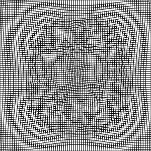
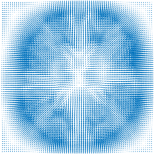
Given a brain-like grid, $\boldsymbol{B}_{o}$, Fig.4(a). Because det$\nabla\boldsymbol{id}=1$ and $\nabla\times\boldsymbol{id}=\boldsymbol{0}$ for the identity map $\boldsymbol{id}$, so $1=f_{o}$, $\boldsymbol{0}=\boldsymbol{g}_{o}$ and $\boldsymbol{B}_{o}=\boldsymbol{\phi}_{o}$ are fed to the algorithm. It is expected to find a transformation that composites $\boldsymbol{B}_{o}$ and outputs $\boldsymbol{id}$. As Fig.4(c) shows, $\boldsymbol{D}$ is found and it left-translates $\boldsymbol{B}_{o}$ to Fig.4(d). Compared it with $\boldsymbol{id}$ in Fig.4(e), the brain-like grid $\boldsymbol{B}_{o}$ is “de-brained”. Fig.4(f) is a guessed identity by reversing the order of $\boldsymbol{B}_{o}$ and $\boldsymbol{D}$ in Fig.4(e). This indicates that $\boldsymbol{D}$ approximates quite accurately to $(\boldsymbol{B}_{o})^{-1}$. $ratio$ had reduced to 0.3%.

(a) $\boldsymbol{B}_{o}$

(b) $\boldsymbol{u}$

(c) $\boldsymbol{D}$

(d) $\boldsymbol{D}\circ\boldsymbol{B}_{o}$

(e) $\boldsymbol{D}\circ\boldsymbol{B}_{o}$ vs $\boldsymbol{id}$

(f) $\boldsymbol{B}_{o}\circ\boldsymbol{D}$ vs $\boldsymbol{id}$

Figure 4: Reconstruct inverse under left-translation

3.3 $\mathbf{Example}$: Inverse Consistency

Given a grid, $\boldsymbol{\Psi}$, of the character “missing