The Pollution-Routing Problem with Speed
Optimization and Uneven Topography

Abstract

This paper considers a joint pollution-routing and speed optimization problem (PRP-SO) where fuel costs and $\text{CO}_{2}e$ emissions depend on the vehicle speed, arc payloads, and road grades. We present two methods, one approximate and one exact, for solving the PRP-SO. The approximate strategy solves large-scale instances of the problem with a tabu search-based metaheuristic coupled with an efficient fixed-sequence speed optimization algorithm. The second strategy consists of a tailored branch-and-price (BP) algorithm in which speed optimization is managed within the pricing problem. We test both methods on modified Solomon benchmarks and newly constructed real-life instance sets. Our BP algorithm solves most instances with up to 50 customers and many instances with 75 and 100 customers. The heuristic is able to find near-optimal solutions to all instances and requires less than one minute of computational time per instance. Results on real-world instances suggest several managerial insights. First, fuel savings of up to 53% are realized when explicitly taking into account arc payloads and road grades. Second, fuel savings and emissions reduction are also achieved by scheduling uphill customers later along the routes. Lastly, we show that ignoring elevation information when planning routes leads to highly inaccurate fuel consumption estimates.
 
Keywords: Network topography; Speed optimization; Branch-and-price; Pollution routing

1 Introduction

Road freight transportation is vital to the functioning of the economy and the supply chain. However, significant negative impacts on people and the environment due to excessive energy usage and considerable greenhouse emissions need to be considered. According to the International Energy Agency (IEA, 2020), global transportation is still responsible for 24% of direct $\text{CO}_{2}$-equivalent ($\text{CO}_{2}e$) emissions from fuel combustion. This is especially true in a city logistics context (Savelsbergh and Van Woensel, 2016).

Over the past years, these observations gave rise to the introduction of pollution- and sustainability-related aspects into traditional Vehicle Routing Problems (VRPs), popularly coined in the literature as the Pollution-Routing Problem (Bektaş and Laporte, 2011). In the literature, similar problems and definitions can be found as the Emissions Minimizing VRPs (EMVRPs) (Raeesi and Zografos, 2019) or Green VRPs (Erdoğan and Miller-Hooks, 2012, Moghdani et al., 2020). These models make use of the fact that the amount of transport-related greenhouse gases (GHGs) emissions is directly proportional to the fuel consumption (Kirby et al., 2000). Multiple factors are considered, including the slope (Suzuki, 2011), vehicle speed (Demir et al., 2012), the payload (Bektaş and Laporte, 2011), traffic congestion (Franceschetti et al., 2013), driver’s operating habit (Bandeira et al., 2013), and the fleet size and mix (Koç et al., 2014).

Specifically, the PRP aims to build routes that minimize an objective function integrating the vehicle’s routing cost (e.g., fuel consumption, the pollution aspect) and the driving costs (e.g., vehicle usage, drivers’ wage, and other direct costs aspect). This paper builds upon this literature and considers modelling the driving costs as fixed costs of vehicles, which is commonly used in heterogeneous vehicle routing problems (see, e.g., Koç et al., 2016), but often disregarded and handled as duration-dependent costs in PRP. Moreover, considering this rich version of the PRP leads to interesting new methodological challenges for speed optimization.

The majority of models describe the road angle, and thus the network topography, as one of the parameters used to formulate the instantaneous engine-out emission rate (Barth and Boriboonsomsin, 2009), but do not consider this further in the model, in the solution methodology or in the results and insights. More specifically, efficient solution methods and extensive computational experiments analyzing the effect of road gradient on fuel consumption and $\text{CO}_{2}e$ emissions are missing in the literature. One notable exception in the same application domain is the paper by Brunner et al. (2019). These authors however assume that speed is constant, which is an unrealistic assumption within a city logistics context (Franceschetti et al., 2013). Concerning vehicle speed, several studies are proposing various optimization procedures. However, there is still a need for efficient and fast speed optimization algorithms to use in exact algorithms.

The contributions of this paper are threefold.

• We introduce the road gradient to the computation of fuel consumption utilizing terrain elevation information. Despite the inclusion of road gradient into the original formulation of fuel consumption, most papers assume a constant road angle for all vehicle trips.

• A number of novel solution approaches are presented, including a branch-and-price algorithm leading to optimal solutions and metaheuristic for larger instances. We develop a novel, fast and efficient algorithm for the vehicle speed optimization.

• We generate important insights based on a broad set of instances to investigate the importance of road gradient on emissions. Additionally, we propose a number of real-life instances.

The remainder of this paper is organized as follows. Section 2 provides a brief review of related scientific literature. In Section 3, we give a detailed description of our PRP model. Section 4 shows the proposed Tabu Search metaheuristic together with a detailed description of the fixed-sequence speed optimization algorithm. Later in Section 5, we present the major components of our branch-and-price algorithm. Section 6 offers extensive computational experiments conducted, and finally, we conclude this research in Section 7.

2 Literature Review

The significant increasing amount of $\text{CO}_{2}e$ emissions derived from road freight transportation has certainly ignited worldwide concerns. Over the last ten years, this resulted in a large body of literature on emissions-aware transportation problems (see, e.g., the survey by Moghdani et al., 2020). The Pollution-Routing Problem (PRP) is an efficient and comprehensive formulation to address the minimization of carbon emissions. The resulting greenhouse emissions of vehicle fuel consumption are the consequence of some influential factors beyond the travel distance (Ericsson, 2001, Brundell-Freij and Ericsson, 2005). According to Demir et al. (2014b), vehicle fuel consumption is affected by multiple factors such as speed, road gradient, road congestion, driver’s operating habit, size and composition (mix) of the vehicle fleet, and payload.

As summarized in Table 1, we observe that some important factors are less studied in previous vehicle routing research, specifically the interaction of load, road gradient, and vehicle speed is missing.

Table 1: Pollution-related Factors Covered by Previous Research on PRPs

Authors	Pollution-related factors (model formulation)				Factors included in the computational analysis	Type of dataset	Solution approach
	load	speed	slope	others
Bektaş and Laporte (2011)	$\surd$	$\surd$	$\surd$		load, speed	UK	CPLEX
Demir et al. (2012)	$\surd$	$\surd$	$\surd$		speed	UK	ALNS
Franceschetti et al. (2013)	$\surd$	$\surd$	$\surd$	$\surd$	departure time, speed, traffic congestion	UK	CPLEX
Demir et al. (2014a)	$\surd$	$\surd$	$\surd$		driving time, speed	UK	ALNS
Koç et al. (2014)	$\surd$	$\surd$	$\surd$	$\surd$	speed, fleet size and mix	UK	HEA
Kramer et al. (2015)		$\surd$		$\surd$	departure time, speed	Modified UK	ILS
Fukasawa et al. (2016)	$\surd$	$\surd$			speed	UK	DCP
Dabia et al. (2017)		$\surd$	$\surd$	$\surd$	start-time, speed	UK	B&P
Rauniyar et al. (2019)	$\surd$	$\surd$			load	UK	NSGA-II
Brunner et al. (2019)	$\surd$		$\surd$		arc slope, fixed load	New dataset	Tailored heuristic
Raeesi and Zografos (2019)	$\surd$	$\surd$	$\surd$	$\surd$	load, fleet size and mix, road congestion	New dataset	CPLEX
Xiao et al. (2020)	$\surd$	$\surd$		$\surd$	travel-arrival-departure- waiting time, speed, load	UK	CPLEX
Proposed work	$\surd$	$\surd$	$\surd$	$\surd$	road gradient, speed, load	Novel dataset	B&P, TS

Abbreviations – CPLEX: IBM Commercial Solver; ALNS: Adaptive Large Neighborhood Search; HEA: Hybrid Evolutionary Algorithm; ILS: Iterated Local Search; DCP: Disjunctive Convex Programming; B&P: Branch and Price; NSGA-II: Non-dominated Sorting Genetic Algorithm; TS: Tabu Search

Road gradient. The road grade (slope) has a significant influence on both the conventional-vehicle fuel economy (Suzuki, 2011) and the electric-vehicle energy consumption (Goeke and Schneider, 2015). The transit of a typical light-duty vehicle over a sloping road surface, with a +6 percent grade, could increase the fuel consumption by 15-20 percent (Boriboonsomsin and Barth, 2009). The influence of hilly roads is undoubtedly more significant on the fuel consumption of heavy-duty trucks. According to Davis et al. (2009), just a minor increase or decrease in road grade (1-4%) can reduce or increase fuel economy by more than 50%. In the case of electric vehicles, the energy consumption is less affected by the road gradient as opposed to conventional vehicles. However, experimental results show the impact of hilly terrain on the electric vehicle miles traveled, confirming that the electric vehicle range in mountainous landscapes is lower (Travesset-Baro et al., 2015).

The road gradient has been mainly studied in PRPs and the so-called Electric Vehicle Routing Problems (E-VRPs). Since the first mathematical formulation of PRPs (Bektaş and Laporte, 2011), the road angle was one of the parameters used to define the instantaneous engine-out emission rate. Table 1 clearly shows that most PRP-previous contributions included the road angle in the mathematical formulation of fuel use rate. This table also stands out two major gaps in the area that the proposed work is trying to address: (i) despite the inclusion of road gradient into the original formulation of fuel consumption, most of the papers assume that the road angle remains constant throughout all vehicle trips, and (ii) the majority of previously generated problem instances have not yet considered the road gradient.

It is worth mentioning that the present work is the first study in the area to create and optimally solve a set of realistic problem instances, which include elevation information for computing the road slopes along the paths.

As mentioned earlier, we found the paper by Brunner et al. (2019) as the only contribution that studied the influence of road grade on fuel consumption. Although these authors considered the slope in their VRP formulation, they assumed a constant road grade for all arcs that form the directed graph. The above does not reflect accurately the hilly topography profile of a road, which typically connects two nodes (arc) with a sequence of multiple uphill/downhill segments. Another assumption in this contribution is related to the vehicle speed. The authors addressed a VRP without time windows, assuming that the vehicles travel through each arc with a given constant speed (input parameter). Last but not least important with respect to the paper assumptions, in Brunner et al. (2019), the payload carried by the vehicle is chosen from a prescribed set of values which means that the authors did not consider the payload as a continuous decision variable.

There are very few papers, outside the application context of PRPs, that take into account the effect of road gradients on fuel consumption. For instance, Tavares et al. (2009) utilizing an exponential regression model (COPERT-III method, introduced by Ntziachristos et al. (2000)) to estimate the minimum fuel consumption during waste collection process. They studied two realistic routing problems showing that the optimal route does not necessarily correspond to the shortest traveled distance. Their computational results demonstrated that significant fuel consumption savings are possible for longer routes with moderate road inclination. Moreover, the contribution of Suzuki (2011) proposed a linear regression model to compute the fuel consumption rate for a heavy-duty truck, based on the fuel-efficiency study of Davis et al. (2009). The author included the road-gradient factor as one of the objective function components (distance and fuel consumption), designed to formulate a traveling salesman problem with time windows.

Concerning the E-VRPs, Yang et al. (2014) performed a numerical simulation. In their paper, the authors used the electric vehicle’s battery (physical model) theory to study the effects of the road’s slope on electricity consumption for both uphill and downhill paths. They concluded that with the increase of the uphill’s tilt angle, each electric vehicle’s electricity consumption increases significantly. Goeke and Schneider (2015) also assumed not-flat terrain with grades in their energy consumption model proposed for electric vehicles. They intensely focused on the effect of load distribution on the performance of commercial electric vehicles. Later, Liu et al. (2017) also investigate the impact of road gradient on the electricity consumption of electric cars. Using 12 gradient ranges and GPS tracking data with a digital elevation map, the authors showed that, in uphill trips, the energy consumption increases almost linearly with the absolute gradient. However, the numerical results also exhibited the positive effect of regenerative braking power acquired during the downhill trips. Finally, Macrina et al. (2019) modeled a comprehensive energy consumption function considering the road gradients. Nevertheless, in their computational study, the authors set the road angle equal to zero for conventional and electric vehicles.

Vehicle speed. Bektaş and Laporte (2011) first addressed the speed of the vehicle in the area of PRPs. In the original formulation of this problem, they explicitly assumed that speed over each arc is chosen from a predefined list of possible values. Koç et al. (2014) also utilized the same discrete speed function but analyzed, for the first time, the effect of fleet size and mix in PRPs. The discretization of vehicle speed was also adopted by Eshtehadi et al. (2017). Here, the authors considered the demand and travel time uncertainty, both aspects addressed by several robust optimization techniques. Moreover, Demir et al. (2012) proposed a specialized speed optimization algorithm (SOA), which computes optimal speeds on a given path so as to minimize fuel consumption, emissions and driver costs. The authors modified the original SOA, which was initially designed for solving the tramp speed optimization problem (Norstad et al., 2011). The speed and traffic congestion were also studied by Franceschetti et al. (2013), originating the time-dependent PRP. This research considers two phases within the planning horizon, the free-transit phase, and the congested phase. One interesting fact of their computational results is that they reduced the emissions cost by waiting at specific locations (stopped vehicles) and avoiding traffic congestion. Kramer et al. (2015) also modified the original SOA providing a new speed and departure time optimization algorithm.

Finally, a huge variety of solution methods has been proposed to solve PRPs. One can find the frequent application of metaheuristics such as ALNS (Demir et al., 2012, 2014a), evolutionary and genetic algorithms (Koç et al., 2014, Rauniyar et al., 2019), and hybrid approaches (Tirkolaee et al., 2020). Table 1 shows the methods used for solving different variants of PRPs. As can be seen, the utilization of exact algorithms in PRPs is very limited. Existing exact methods often approximated or discretized the vehicle speeds in order to reduce the complexity. Fukasawa et al. (2016) resolved the issues of speed discretization by introducing a formulation framework to directly incorporate the nonlinear relationship between cost and speed into the PRP. They employed different tools from disjunctive convex programming to find a set of vehicle speeds over the routes, minimizing the total cost (operational and environmental) and respecting the constraints on time and vehicle capacities. More recently, vehicle speed has been computed using continuous optimization on PRP. Here Xiao et al. (2020) introduced the continuous PRP ($\epsilon$-CPRP) where the travel time, load flow, departing/arrival/waiting times, and driving speed were treated as continuous decision variables. The authors developed an $\epsilon$-accurate inner polyhedral approximation method for linearizing the original fuel consumption equation (Bektaş and Laporte, 2011), and solved the PRP instances with up to 25 customers.

To the best of our knowledge, Dabia et al. (2017) is the only previous contribution that addressed a complex variant of PRP, and developed an exact branch-and-price algorithm. To address speed optimization within the pricing subproblem, the authors introduced a ready-time function for updating the speed-dependent routing costs within a bidirectional labeling algorithm. We propose an improved branch-and-price method that uses a novel speed optimization algorithm.

In Dabia et al. (2017), a complex ready time function has to be solved recursively for determining the optimal speed that minimizes the routing cost of a partial path, which can be computationally expensive. In our proposed labeling algorithm, the optimal speed can be determined efficiently and without full “backtracking” of the partial path. In addition, we have also developed completion bounds that further improved the efficiency of solving the pricing subproblem.

3 Problem Formulation

In Section 3.1, we formulate the carbon dioxide equivalent ($\text{CO}_{2}e$) emission using the comprehensive modal emissions model (CMEM). In Section 3.2, we introduce a mixed-integer linear programming formulation for the joint Pollution Routing and Speed Optimization problem (PRP-SO).

3.1 Modelling $\text{CO}_{2}e$ emissions

We model $\text{CO}_{2}e$ emissions using the CMEM (refers to e.g. Barth and Boriboonsomsin (2009), Boriboonsomsin and Barth (2009), Demir et al. (2012)). The parameters and the values for light, medium, and heavy-duty vehicles (denoted respectively as LDV, MDV, HDV) we used in our experiments are shown in Table 2.

Table 2: Comprehensive Modal Emissions Model (CMEM)

Symbol	Description	LDV	MDV	HDV
$F_{k}$	Engine friction factor (kJ/rev/liter)	0.23	0.20	0.17
$N_{k}$	Engine speed (rev/s)	35	34	33
$V_{k}$	Engine displacement (liters)	3	7	11
$A_{k}$	Frontal surface area of a vehicle (m2)	5	7.6	8.2
$C^{d}_{k}$	Aerodynamic drag coefficients	0.32	0.55	0.70
$C^{r}_{k}$	Rolling resistance coefficients	0.01	0.009	0.008
$r_{k}$	Vehicle acceleration (m$/$s2)	0	0	0
$w_{k}$	Curb weight (kg)	2,300	5,500	13,000
$\kappa$	Heating value for diesel fuel (kJ/g)	45	45	45
$\varepsilon$	Vehicle drive train efficiency	0.4	0.4	0.4
$\varpi$	Efficiency parameter for diesel engines	0.9	0.9	0.9
$\xi$	Fuel-to-air mass ratio	1	1	1
$\psi$	Conversion factor from grams to liters	737	737	737
$\rho$	Air density (kg/m3)	1.2041	1.2041	1.2041
$g$	Gravity (m$/$s2)	9.81	9.81	9.81

According to the CMEM model, the instantaneous fuel use rate of a vehicle $k$ when traveling at a constant speed $\nu_{k}$ with payload $x$ on a path with the road angle $\phi$ is given by

$$\frac{\xi}{\kappa\psi}\Big{(}F_{k}N_{k}V_{k}+\frac{0.5C^{d}_{k}A_{k}\rho\nu_{k}^{3}+(w_{k}+x)\nu_{k}(r_{k}+gsin\ \phi+gC^{r}_{k}\ cos\ \phi)}{1000\varepsilon\varpi}\Big{)}$$

When traversing a distance of $d$ meters, the amount of fuel consumption is therefore given by

$$\frac{\xi F_{k}N_{k}V_{k}}{\kappa\psi}\frac{d}{\nu_{k}}+\frac{1}{1000\varepsilon\varpi}(r_{k}+g\ sin\ \phi+g\ C^{r}_{k}\ cos\ \phi)(w_{k}+x)(d)+\frac{0.5C^{d}_{k}A_{k}\rho}{1000\varepsilon\varpi}d\nu_{k}^{2}$$

Now that, there are a sequence of road segments associated on each arc $e$ which are denoted by $S_{e}$. Let $d_{es}$ denote the travel distance of segment $s\in S_{e}$, and $x_{ke}$ denote the payload of vehicle $k$ when traversing arc $e$. For traversing the sequence of road segments associated on arc $e$, the amount of fuel consumption of vehicle $k$ can then be determined by

$$\alpha_{ke}\frac{1}{\nu_{k}}+\beta_{ke}(w_{k}+x_{ke})+\gamma_{ke}\nu_{k}^{2}$$ (1)

where

$$\alpha_{ke}=\frac{\xi F_{k}N_{k}V_{k}\sum_{s\in S_{e}}d_{es}}{\kappa\psi}$$ (2)

$$\beta_{ke}=\frac{\xi\sum_{s\in S_{e}}d_{es}(r_{k}+g\ sin\ \phi_{es}+g\ C^{r}_{k}\ cos\ \phi_{es})}{1000\varepsilon\varpi\kappa\psi}$$ (3)

$$\gamma_{ke}=\frac{0.5\xi C^{d}_{k}A_{k}\rho\sum_{s\in S_{e}}d_{es}}{1000\varepsilon\varpi\kappa\psi}$$ (4)

To speed up the $\text{CO}_{2}e$ emission calculations, we precompute the parameters $\alpha_{ke}$, $\beta_{ke}$, and $\gamma_{ke}$ for all the vehicles $k$ and arcs $e$. These parameters are used in formulating the mathematical model in Section 3.2 and developing the solution approaches in Section 4 and Section 5.

3.2 Mathematical model

Table 3: Notation for the MINLP Model

Symbol	Description	Domain
$\cal K$	Set of vehicles	index set
$\cal N$	Set of nodes representing $n$ customers and the depot	index set
$\cal A$	Set of arcs	index set
$q_{i}$	Demand of customer $i$	$\mathbb{Z}^{+}$
$w_{k}$	Curb weight of vehicle $k$	$\mathbb{Z}^{+}$
$Q_{k}$	Capacity of vehicle $k$	$\mathbb{Z}^{+}$
$e_{i}$	Earliest start time at customer $i$	$\mathbb{R}^{+}$
$l_{i}$	Latest start time at customer $i$	$\mathbb{R}^{+}$
$s_{i}$	Service time at customer $i$	$\mathbb{R}^{+}$
$f_{k}$	Fixed cost of vehicle $k$	$\mathbb{R}^{+}$
$c_{k}$	Variable cost of vehicle $k$ including fuel and $\text{CO}_{2}e$ emission costs	$\mathbb{R}^{+}$
$a_{k}$	Lower limit of the speed of vehicle $k$	$\mathbb{R}^{+}$
$b_{k}$	Upper limit of the speed of vehicle $k$	$\mathbb{R}^{+}$
$d_{e}$	Distance of arc $e$	$\mathbb{R}^{+}$
$\alpha_{ke}$	A constant for estimating the fuel consumption of vehicle $k$ on arc $e$	$\mathbb{R}^{+}$
$\beta_{ke}$	A constant for estimating the fuel consumption of vehicle $k$ on arc $e$	$\mathbb{R}^{+}$
$\gamma_{ke}$	A constant for estimating the fuel consumption of vehicle $k$ on arc $e$	$\mathbb{R}^{+}$
$z_{ki}$	Decision variable, to allocate customers to vehicles	$\mathbb{B}$
$y_{ke}$	Decision variable, to allocate arcs to vehicles	$\mathbb{B}$
$x_{ke}$	Decision variable, payload of vehicle $k$ when traversing on arc $e$	$\mathbb{R}^{+}$
$t_{ki}$	Decision variable, time at which vehicle $k$ starts serving customer $i$	$\mathbb{R}^{+}$
$\nu_{k}$	Decision variable, speed of vehicle $k$	$\mathbb{R}^{+}$

Let $\cal K$ be the set of vehicles. Let $G({\cal N},{\cal A})$ be the underlying directed graph. A set of nodes ${\cal N}=\{0,1,...,n\}$ contains $n$ customers and a depot (represented by node 0). The set of arcs ${\cal A}$, defined as $\{(i,j)\in{\cal N}\times{\cal N}:i\not=j\}$, represents the paths between the nodes. Each node $i\in\cal N$ is associated with a demand $q_{i}$ and a time window [$e_{i}$, $l_{i}$]. Each vehicle $k\in\cal K$ is associated with a fixed cost $f_{k}$, a variable cost $c_{k}$ (including the costs for $\text{CO}_{2}e$ emission and fuel consumption), a vehicle capacity $Q_{k}$, vehicle curb weight $w_{k}$, and speed limits [$a_{k}$, $b_{k}$]. Each arc $e\in{\cal A}$ is associated with a distance $d_{e}$, and the parameters $\alpha_{ke}$, $\beta_{ke}$ and $\gamma_{ke}$ described in Section 3.1 for estimating fuel consumption.

For all $k\in\cal K$ and $i\in{\cal N}$, let $z_{ki}$ be a binary decision variable, with $z_{ki}=1$ if and only if customer $i\in{\cal N}\setminus\{0\}$ is served by vehicle $k$; and with $z_{k0}=1$ if and only if vehicle $k$ is in use. For all $k\in\cal K$ and $e\in{\cal A}$, let $y_{ke}$ be a binary decision variable with $y_{ke}=1$ if and only if vehicle $k$ traverses arc $e$, and let $x_{ke}$ denote the corresponding payload when vehicle $k$ traverses arc $e$. For all $k\in\cal K$ and $i\in{\cal N}$, let $t_{ki}$ denote the time at which vehicle $k$ starts serving customer $i\in{\cal N}\setminus\{0\}$; and let $t_{k0}$ denote the time vehicle $k$ returns to the depot. For all $k\in\cal K$, let $\nu_{k}$ denote the speed of vehicle $k$.

The objective is to minimize the total $\text{CO}_{2}e$ emission costs, fuel costs, and vehicle fixed costs, subject to the following constraints: i) the total demand in a vehicle does not exceed the vehicle capacity; ii) every route starts and ends at the vehicle’s home depot; iii) every customer is visited exactly once by exactly one vehicle; iv) all vehicles should return to its home depot within a time limit; v) every vehicle travels at a speed within the speed limits.

The joint Pollution Routing and Speed Optimization problem (PRP-SO) can be formulated as the following nonlinear integer programming model.

$$(\text{PRP-SO}):$$

min $$\sum\limits_{k\in{\cal K}}f_{k}z_{k0}+\sum\limits_{k\in{\cal K}}\sum\limits_{e\in{\cal A}}c_{k}y_{ke}\Big{(}\frac{\alpha_{ke}}{\nu_{k}}+\beta_{ke}w_{k}+\beta_{ke}x_{ke}+\gamma_{ke}\nu_{k}^{2}\Big{)},$$ (5)

s.t. $$\sum\limits_{k\in{\cal K}}z_{ki}=1, \forall i\in{\cal N}\setminus\{0\},$$ (6)

$$\sum\limits_{e\in\delta^{+}(i)}y_{ke}=\sum\limits_{e\in\delta^{-}(i)}y_{ke}=z_{ki}, \forall k\in{\cal K},i\in{\cal N},$$ (7)

$$\sum\limits_{e\in\delta^{-}(i)}x_{ke}-\sum\limits_{e\in\delta^{+}(i)}x_{ke}=q_{i}z_{ki}, \forall k\in{\cal K},i\in{\cal N}\setminus\{0\},$$ (8)

$$x_{ke}\leq(Q_{k}-q_{i})y_{ke}, \forall k\in{\cal K},e=(i,j)\in\cal A,$$ (9)

$$t_{kj}-t_{ki}\geq s_{i}+d_{e}\ \frac{y_{ke}}{\nu_{k}}-l_{0}\Big{(}1-y_{ke}\Big{)}, \forall k\in{\cal K},e=(i,j)\in{\cal A}:j\neq 0,$$ (10)

$$e_{i}z_{ki}\leq t_{ki}\leq l_{i}z_{ki}, \forall k\in{\cal K},i\in{\cal N}\setminus\{0\},$$ (11)

$$t_{ki}+s_{i}+d_{e}\ \frac{y_{ke}}{\nu_{k}}\leq l_{0}, \forall k\in{\cal K},i\in{\cal N}\setminus\{0\},e=(i,0)$$ (12)

$$a_{k}\leq\nu_{k}\leq b_{k}, \forall k\in{\cal K},$$ (13)

$$\nu_{k}\in\mathbb{R}^{+}, \forall k\in{\cal K},$$ (14)

$$t_{ki}\in\mathbb{R}^{+}, \forall k\in{\cal K},i\in{\cal N},$$ (15)

$$x_{ke}\in\mathbb{R}^{+}, \forall k\in{\cal K},e\in{\cal A},$$ (16)

$$y_{ke}\in\{0,1\}, \forall k\in{\cal K},e\in{\cal A},$$ (17)

$$z_{ki}\in\{0,1\}, \forall k\in{\cal K},i\in{\cal N}.$$ (18)

The objective function (5) minimizes the total vehicle fixed costs, fuel consumption costs, and $\text{CO}_{2}e$ emission costs. Constraints (6) - (7) ensure that each customer is visited once by exactly one vehicle. Constraints (8) are the flow conservation constraints. Constraints (9) ensure that the payload does not exceed vehicle capacity. Constraints (10) - (12) ensure that customers are visited within the given time windows. Constraints (13) ensure that vehicles travel at a speed within the limits.

4 Metaheuristic

Metaheuristic approaches require frequently evaluating solutions with fixed vehicle routes. We present an efficient algorithm for finding the optimal vehicle speed of a given route so that we can compute the costs of $\text{CO}_{2}e$ emissions and fuel consumption efficiently. In Section 4.1, we present a novel polynomial-time algorithm for solving the fixed-sequence speed optimization subproblem — determine the optimal speed of a vehicle when the customer sequence is fixed. To demonstrate the effectiveness of the speed optimization algorithm, it is embedded into a Tabu Search (TS) metaheuristic for our experiments. TS is originally proposed by Glover (1986) as a synthesis of the perspectives of operations research and artificial intelligence. TS has been widely used and has been shown to be effective for finding near-optimal solutions to vehicle routing problems, see, e.g. Gendreau et al. (1994), Toth and Vigo (2003), Lai et al. (2016). Review on the recent development of TS can refer to Gendreau and Potvin (2019). Major components of the proposed TS include the fixed-sequence speed optimization subproblem in Section 4.1, the penalized objective function in Section 4.2, the initial solutions in Section 4.3, the neighborhood structure in Section 4.4, the intra-route improvement procedure in Section 4.5, and the search procedure in Section 4.6.

4.1 Fixed-sequence speed optimization subproblem

The fixed-sequence speed optimization subproblem determines the optimal speed of a vehicle for a given customer sequence. Let $R=(v_{1},v_{2},...,v_{n})$ denote a fixed sequence of nodes in a vehicle route where both $v_{1}$ and $v_{n}$ represent the home depot.

Without time-window constraints, vehicles should always travel at a speed that is most cost-efficient and within the speed limits of the vehicle. The most cost-efficient speed of vehicle $k$ when there are no time window constraints is given by

$$\bar{v}_{k}=\sqrt[3]{\frac{\xi_{k}F_{k}N_{k}V_{k}1000\varepsilon_{k}\varpi_{k}}{C^{d}_{k}A_{k}\rho_{k}}}$$

Since $\bar{v}_{k}$ is independent of the vehicle route when there are no time window constraints, the optimal speed of vehicle $k$ within speed limits $[a_{k},b_{k}]$ can be computed by

$$v^{*}_{k}=\begin{cases}\bar{v}_{k},&\text{if $a_{k}\leq\bar{v}_{k}\leq b_{k}$},\\ a_{k},&\text{if $\bar{v}_{k}\leq a_{k}$},\\ b_{k},&\text{if $\bar{v}_{k}\geq b_{k}$}.\end{cases}$$

In the presence of time window constraints, a vehicle should travel at a speed that satisfies all time window constraints and incurs a minimal cost. Let $\sigma(R)$ denote the lowest vehicle speed without violating any time windows associated on the nodes of route $R$. When a vehicle travels at the speed of $\sigma(R)$ in route $R$, all time window constraints will be satisfied. We will show in Proposition 1 that $\sigma(R)$ can be computed efficiently by

$$\sigma(R)=\max_{i,j\in\{1,2,...,|R|\}:i<j}\frac{\Delta(j)-\Delta(i)}{l_{v_{j}}-e_{v_{i}}-S_{ij}}$$ (19)

where $\Delta(i)=\sum_{l=1}^{i-1}d_{v_{l},v_{l+1}}$ denotes the total distance from the depot to node $i$ along vehicle route $R$, $S_{ij}=\sum_{k=i}^{j-1}s_{v_{k}}$ denotes the total service time from node $v_{i}$ to node $v_{j-1}$ along vehicle route $R$, and that $[e_{v},l_{v}]$ is the time window associated on node $v$. If $\sigma(R)\leq 0$, no feasible speed exists due to conflicting time window constraints.

Since a vehicle can wait at the customer node if the vehicle arrives earlier than the lower bound of a time window, any speed that is greater than $\sigma(R)$ also satisfies the time-window constraints in route $R$. Thus, the optimal speed of vehicle $k$ when traversing on route $R$ is given by

$$\max(v^{*}_{k},\ \sigma(R))$$ (20)

The total cost (as defined in the objective function (5)) of a given solution can be evaluated straightforward when the optimal speeds of the vehicle routes have been found by using (19) and (20).

Proposition 1.

The minimum speed without violating any time window constraints of a vehicle route $R$ is given by $\sigma(R)$ when $\sigma(R)>0$, and can be obtained in a $O(n^{2})$ complexity where $n$ is the number of nodes in route $R$.

Proof.

Let $R=(v_{1},v_{2},...,v_{n})$ denote the sequence of nodes in a vehicle route $R$ with both $v_{1}$ and $v_{n}$ representing the home depot, and there is at least one customer node in $R$ i.e. $n\geq 3$. Furthermore, we assume that the nodes in $R$ are not all located at the same location. For $i=2,...,n$, let $\Delta(i)=\sum_{l=1}^{i-1}d_{v_{l},v_{l+1}}$ denote the total distance from node $v_{1}$ (the depot) to node $v_{i}$ along vehicle route $R$. Set $\Delta(1)=0$. For all $i=1,2,...,n$ and $j=2,...,n$, with $i<j$, let $S_{ij}=\sum_{k=i}^{j-1}s_{v_{k}}$ denote the total service time from node $v_{i}$ to node $v_{j-1}$. For every distinct pair of nodes $i,j\in\{1,2,...,n\}$, with $i<j$, the following lower bound of $\sigma(R)$ can be derived:

$$\frac{\Delta(j)-\Delta(i)}{l_{v_{j}}-e_{v_{i}}-S_{ij}}$$

Any vehicle speed that is higher than the above lower bound induced from nodes $i$ and $j$ would violate one of the time window constraints associated on nodes $v_{i}$ and $v_{j}$.

The minimum speed without violating any time window constraints in $R$ is given by the maximum lower bounds for all distinct pairs of nodes, and thus we have

$$\sigma(R)=\max_{i,j\in\{1,2,...,|R|\}:i<j}\frac{\Delta(j)-\Delta(i)}{l_{v_{j}}-e_{v_{i}}-S_{ij}}.$$

Since there are $\frac{n(n-1)}{2}$ distinct pairs of nodes in a vehicle route of length $n$, $\sigma(R)$ can be computed in $O(n^{2})$.

To complete the proof, we will show that a pair of conflicting time window constraints exist in route $R$ if and only if $\sigma(R)\leq 0$. Consider two cases: i) $\sigma(R)<0$; ii) $\sigma(R)=0$. Case i: By definition we have $\Delta(j)-\Delta(i)\geq 0$ for all $i,j=1,...,n$ with $i<j$. Therefore, $\sigma(R)<0$ iff there exist $v_{i}$ and $v_{j}$ with $l_{v_{j}}-e_{v_{i}}<S_{ij}$ which implies a violation on one of the time window constraints associated on nodes $v_{i}$ and $v_{j}$. Case ii: Suppose the contrary, we consider a vehicle with a speed equals to zero and that all the time window constraints in $R$ are satisfied. Since the due date $l_{v}\neq\infty$ for all $v$, we have $\sigma(R)=0$ iff $\Delta(j)-\Delta(i)=0$ for all $i,j=1,...,n$ with $i<j$. Since the nodes in $R$ are not all located at the same location, there exist two distinct nodes $v_{i}$ and $v_{j}$ in $R$ with $d_{v_{i},v_{j}}>0$ and $i<j$. This implies that, there exist $v_{i}$ and $v_{j}$ in $R$ with $i<j$ and $\Delta(j)-\Delta(i)>0$ which leads to a contradiction. ∎

4.2 Penalized objective function

We allow infeasible solutions in the search space. It is implemented as a penalized objective function that is obtained by relaxing some of the constraints and incorporating them into the objective function with the use of self-adjusting penalty parameters.

If a vehicle $k\in\cal K$ is assigned to a non-empty route $R$, and is travelling at a speed of $\nu_{k}$, the travel cost $c(R)$ can be written as $c(R)=f_{k}+\sum_{e\in{\cal A}(R)}c_{k}\big{(}\frac{\alpha_{ke}}{\nu_{k}}+\beta_{ke}w_{k}+\beta_{ke}\bar{x}_{ke}+\gamma_{ke}\nu_{k}^{2}\big{)}$ where $\bar{x}_{ke}$ is the payload of vehicle $k$ on arc $e$ and ${\cal A}(R)$ denotes the arcs on route $R$. The overload $\text{P}(R)$ representing the violation of the vehicle capacity constraints is defined as $\text{P}(R)=\big{[}\sum_{i\in{\cal N}(R)}q_{i}-Q_{k}\big{]}^{+}$ where ${\cal N}(R)$ denotes the customer nodes on route $R$. After incorporating the penalties for possible violations, the penalized objective function value is computed by $z(R)=c(R)+\rho\text{P}(R)$ where $\rho\in\mathbb{R}^{+}$ is the penalty weight that is self-adjusting in the search. The penalty weight $\rho$ is initialized as 1, and updated in every $\delta$ iterations as follows. If $\text{P}(R)=0$ for all vehicle routes $R$, then update $\rho$ to $0.5\rho$; otherwise, update $\rho$ to $2\rho$.

4.3 Initial solution

The initial solution is created by first applying a stochastic insertion-based heuristic and then improved by using the TS procedure described in Algorithm 1 with a limited number of iterations. The number of iterations is set to $\lceil I_{1}n\rceil$ where $I_{1}$ is a user-controlled parameter and $n$ is the number of customers. After creating ten such initial solutions, the best one is returned as the initial solution for the main search procedure described in Section 4.6.

The following stochastic insertion-based heuristic is applied. It begins by assigning exactly one arbitrarily selected customer to each of the randomly selected $l$ vehicles, where $l$ is a randomly generated integer between 1 and the total number of vehicles available. Then, the remaining customers are considered one by one, following a randomized order. For each customer, all possible locations in all routes are evaluated for insertion, and the customer is subsequently inserted into a vehicle route at the position that minimizes the insertion cost (the incremental change in the penalized objective function value). We determine the insertion costs by using the algorithm described in Section 4.1 that performs speed optimization for a fixed sequence of nodes on a route.

4.4 Neighborhood structure

Let $\mathcal{X}$ denote the set of all feasible solutions for the instance. We define the solutions in the neighborhood of a given solution $x\in\mathcal{X}$ as $\textbf{N}(x)$. At each iteration, all possible move operations for all customers are evaluated and the best one is subsequently performed. The move operation involves relocating a customer from its current route to another route at the location that minimizes the insertion cost. The insertion cost is determined by applying the speed optimization algorithm described in Section 4.1. The best move operation is the one that leads to the lowest total penalized objective function value and the following diversification penalty. For a given solution $x\in\mathcal{X}$, we define the diversification penalty as $\phi(x)=\lambda c(x)\sqrt{n}\vartheta_{ir}$ where $n$ is the number of customers, $\vartheta_{ir}$ counts the number of times customer $i$ has been moved to route $r$ so far in the search, and $\lambda$ is a positive parameter that controls the intensity of diversification. Readers can refer to Soriano and Gendreau (1996) for extensive discussion on diversification schemes.

To prevent cycling, if a customer has been moved from route $r$ to route $s$ in a given iteration, then moving the same customer back to route $r$ is declared tabu which implies that this reverse operation is forbidden for the next $\lceil h\ \text{log}_{10}(n)\rceil$ iterations where $h$ is a user-controlled parameter and $n$ is the number of customers. To prevent the search from stagnating, the following aspiration criterion is applied: a Tabu move is allowed only when the resulting solution is feasible and has an objective function value that is better than that of the current best feasible solution found by the search.

4.5 Intra-route improvement procedure

The following procedure is applied for improving the solution by modifying customers’ position within the same route: a customer is randomly picked and then reinserted into the best location of the same route, until no further improvement is possible. The intra-route improvement procedure is invoked after the selected move operation is performed, the parameter for overload penalty is updated, or when the best feasible solution is improved.

4.6 Search procedure

The TS routine is presented in Algorithm 1. The search procedure consists of two phases. The first phase of the procedure starts by constructing an initial solution as described in Section 4.3. Next, the best solution found in the first phase is improved in the second phase by executing $I_{2}$ iterations of the TS routine.

Algorithm 1 Tabu Search

1:input: initial solution $x_{0}$

2:Set $x=x_{0}$. If $x$ is feasible, set $z^{*}=c(x)$ and $x^{*}=x$; otherwise, set $z^{*}=\infty$ and $x^{*}=x$.

3:determine $z(\bar{x})$ and $\phi(\bar{x})$ for all $\bar{x}\in{\cal N}(x)$

4:while stopping condition is not satisfied do

5:     select $\bar{x}\in{\cal N}(x)$ that

6:     - minimizes $z(\bar{x})$ + $\phi(\bar{x})$

7:     - $\bar{x}$ is non-tabu or it satisfies the aspiration criteria

8:     set the reverse move tabu for $\theta$ iterations

9:     perform the intra-route improvement procedure on $\bar{x}$.

10:     if $\bar{x}$ is feasible and $z(\bar{x})<z^{*}$ then set $x^{*}={\bar{x}}$ and $z^{*}=z(\bar{x})$.      

11:     set $x=\bar{x}$, and update the penalty weight of overload for every $\delta$ iterations

12:     update $z(\bar{x})$ and $\phi(\bar{x})$ for all $\bar{x}\in\textbf{N}(x)$

13:return $x^{*}$

Algorithm 1 shows the TS procedure. In line 2, the algorithm starts with an initial solution $x_{0}$ which is obtained by running the TS routine with $I_{1}$ iterations as described in Section 4.3. In line 3, the penalized objective function and diversification penalty associated on all the move operations are updated. The loop in lines 4–12 is then invoked and stops until after $I_{2}$ iterations. In line 5–7, the best neighborhood solution is picked which takes into account the diversification penalty, overload penalty, solutions in the Tabu list, and the aspiration criteria. As described in Section 4.4, the diversification penalty $\phi(x)$ depends on the intensification parameter $\lambda$. In line 8, the reverse move is forbidden for the next $\lceil h\ \text{log}_{10}(n)\rceil$ iterations. As shown in lines 9–10, the intra-route improvement procedure described in Section 4.5 is performed on the two routes that are modified in the best neighborhood solution. The incumbent is updated if a new best feasible solution is identified. In lines 11–12, the search moves to the selected neighboring solution. The penalty weight of overload is updated in every $\delta$ iterations. Whenever the search moves to a neighboring solution, the penalized objective function and diversification penalty associated on each of the move operations are again updated by using the speed optimization algorithm described in Section 4.1 and the penalized objective function defined in Section 4.2. The computational time is manageable since we only need to update the costs of the move operations that are involved with the modified routes. The values for the algorithmic parameters in the search procedure include $I_{1}$, $I_{2}$, $\lambda$, $h$ and $\delta$ which are set according to the parameter tuning experiment described in Section 6.3.

5 Branch-and-price Algorithm

Branch-and-price is a successful exact method for solving several VRP variants. It relies on reformulating the problem as a set-partitioning (SP) problem and applying branch-and-bound to solve the SP formulation, which is known to provide tight linear bounds. As the number of variables in the SP model grows exponentially with the instance size, column generation is applied to identify profitable variables and add them to the model dynamically. For a review of branch-and-price applied to vehicle routing we refer to Costa et al. (2019). In this section, we present the SP-based PRP-SO formulation and describe our branch-and-price solution method, with a focus on the specialized algorithm for solving the non-linear column generation subproblem.

5.1 Set-partitioning formulation

A route $p$ is feasible for vehicle $k$ when i) there exists a value $\nu\in[a_{k},b_{k}]$ such that no time-window constraint is violated when vehicle $k$ executes route $p$ at speed $\nu$; and ii) the total demand of the customers served along $p$ does not exceed the vehicle capacity $Q_{k}$. Let $\Omega_{k}$ be the set of feasible routes for vehicle $k$. Furthermore, for each $p\in\Omega_{k}$, let $c_{p}^{k}$ be the cost incurred when vehicle $k$ executes route $p$ at the optimal speed, as defined in Section 4.1. Finally, for each route $p\in\Omega_{k}$ and customer $i\in{\cal N}\setminus\{0\}$, let

$$\delta_{ip}=\begin{cases}1,&\text{if route $p$ visits customer $i$,}\\ 0,&\text{otherwise.}\end{cases}$$

We define binary decision variables $\lambda_{p}^{k}$ for all $k\in\cal K$ and $p\in\Omega_{k}$, such that $\lambda_{p}^{k}=1$ if and only if vehicle $k$ executes route $p$ in the solution. Then, the PRP-SO is formulated as the following SP problem:

$$(\text{SP}):\ \min\ \sum\limits_{k\in{\cal K}}\sum\limits_{p\in\Omega_{k}}c_{p}^{k}\lambda^{k}_{p},$$ (21)

s.t. $$\sum\limits_{k\in{\cal K}}\sum\limits_{p\in\Omega_{k}}\delta_{ip}\lambda_{p}^{k}=1, \forall i\in{\cal N}\setminus\{0\},$$ (22)

$$\sum\limits_{p\in\Omega_{k}}\lambda^{k}_{p}\leq 1, \forall k\in\cal K,$$ (23)

$$\lambda_{p}^{k}\in\{0,1\}, \forall k\in{\cal K},\forall p\in\Omega_{k}.$$ (24)

The objective function (21) minimizes the total costs. Constraints (22) ensure that each customer is visited exactly once, and constraints (23) enforce a maximum of one route per vehicle.

5.2 Column generation subproblem

The restricted master problem (RMP) refers to the linear relaxation of (21)-(24) with a restricted set of vehicle routes. Let $\pi_{i}$, $i\in{\cal N}\setminus\{0\}$, be the dual prices associated with constraints (22) after solving the RMP. The pricing problem for vehicle $k$ is defined as follows:

$$\text{($\text{PP}$)}:\ \min\ f_{k}+c_{k}\sum\limits_{e\in{\cal A}}\Big{(}\frac{\alpha_{ke}}{\nu}+\beta_{ke}(w_{k}+x_{e})+\gamma_{ke}\nu^{2}\Big{)}y_{e}-\sum\limits_{i\in{\cal N}\setminus\{0\}}\pi_{i}z_{i},$$ (25)

$$\text{s.t}.\ \ \sum\limits_{e\in\delta^{+}(i)}y_{e}=\sum\limits_{e\in\delta^{-}(i)}y_{e}=z_{i}, \forall i\in{\cal N}\setminus\{0\},$$ (26)

$$\sum\limits_{e\in\delta^{+}(0)}y_{e}=\sum\limits_{e\in\delta^{-}(0)}y_{e}=1,$$ (27)

$$\sum\limits_{e\in\delta^{-}(i)}x_{e}-\sum\limits_{e\in\delta^{+}(i)}x_{e}=q_{i}z_{i}, \forall i\in{\cal N}\setminus\{0\},$$ (28)

$$x_{e}\leq(Q_{k}-q_{i})y_{e}, \forall e=(i,j)\in\cal A,$$ (29)

$$\sum\limits_{i\in{\cal N}\setminus\{0\}}q_{i}z_{i}\leq Q_{k},$$ (30)

$$t_{j}-t_{i}\geq s_{i}+d_{e}\ \frac{y_{e}}{\nu}-l_{0}\Big{(}1-y_{e}\Big{)}, \forall e=(i,j)\in{\cal A}:j\neq 0,$$ (31)

$$e_{i}z_{i}\leq t_{i}\leq l_{i}z_{i}, \forall i\in{\cal N}\setminus\{0\},$$ (32)

$$t_{i}+s_{i}+d_{e}\ \frac{y_{e}}{\nu}\leq l_{0}, \forall i\in{\cal N}\setminus\{0\},e=(i,0),$$ (33)

$$\nu\in[a_{k},b_{k}],$$ (34)

$$t_{i}\in\mathbb{R}^{+}, \forall i\in{\cal N},$$ (35)

$$x_{e}\in\mathbb{R}^{+}, \forall e\in{\cal A},$$ (36)

$$y_{e}\in\{0,1\}, \forall e\in{\cal A},$$ (37)

$$z_{i}\in\{0,1\}, \forall i\in{\cal N}\setminus\{0\}.$$ (38)

The objective function (25) minimizes the route-dependent costs (including vehicle fixed cost and $\text{CO}_{2}e$ emissions cost) and the dual prices of the RMP. Constraints (26)-(27) are the flow conservation constraints. Constraints (28)-(29) keep track of the payload in the vehicle along each arc traversed. Constraint (30) is the vehicle capacity constraint. Constraints (31)-(33) are the time window constraints. Finally, constraint (34) ensures that the vehicle travels at a speed within the prescribed limits.

5.3 Pricing algorithm

The pricing algorithm identifies columns with a negative reduced cost, that is, it finds solutions to (PP) with a negative objective value. As common in branch-and-price for vehicle routing, we solve the pricing problem with a labeling algorithm. A label represents a partial route from the depot to a customer. Label extensions are created by extending labels to all feasible customers. Table 4 summarizes the attributes of a label alongside their corresponding initialization values and updating rules.

Table 4: Pricing Algorithm: Label Attributes, Initialization Values and Updating Rules

Attributea	Description	Initializationb	Updating rulec
$N_{P}$	Set of customers	$\{i\}$	$N_{Q}=N_{P}\cup\{j\}$
$n_{P}$	Last customer served	$i$	$j$
$q_{P}$	Total demand	$q_{i}$	$q_{Q}=q_{P}+q_{j}$
$D_{P}$	Total distance traveled	$d_{e}$	$D_{Q}=D_{P}+d_{e}$
$\tau_{P}$	Earliest departure time assuming maximum speed	$\max(e_{i},d_{e}/b_{k})+s_{i}$	$\tau_{Q}=\max(e_{j},\tau_{P}+d_{e}/b_{k})+s_{j}$
$S_{P}$	Total service time before $n_{P}$	0	$S_{Q}=S_{P}+s_{n_{P}}$
${\cal T}_{P}$	Triples of distance, total service time and earliest service time for calculating $\sigma_{P}$	$\{(d_{e},0,e_{i})\}$	${\cal T}_{Q}={\cal T}_{P}\cup\{(D_{Q},S_{Q},e_{j})\}$
$\sigma_{P}$	Minimum vehicle speed such that all time windows are respected	$d_{e}/l_{i}$	$\sigma_{Q}=\max\limits_{(d,s,t)\in{\cal T}_{P}}\frac{D_{Q}-d}{l_{j}-t-(S_{Q}-s)}$
$\nu_{P}$	Optimal speed	$\max(v^{*}_{k},d_{e}/l_{i})$	$\nu_{Q}=\max(v^{*}_{k},\sigma_{Q})$
$\alpha_{P}$ $\beta_{P}$ $\gamma_{P}$ $\delta_{P}$	Coefficients for $\text{CO}_{2}e$ emissions	$\alpha_{ke}$ $\beta_{ke}$ $\gamma_{ke}$ $\beta_{P}q_{i}$	$\alpha_{Q}=\alpha_{P}+\alpha_{ke}$ $\beta_{Q}=\beta_{P}+\beta_{ke}$ $\gamma_{Q}=\gamma_{P}+\gamma_{ke}$ $\delta_{Q}=\delta_{P}+\beta_{Q}q_{j}$

^a Assuming label $P$; ^b Assuming vehicle $k$ and a label representing the partial route along arc $e=(0,i)$; ^c Assuming label $Q$ obtained by extending $P$ along arc $e=(i,j)$.

A key component of our pricing algorithm is the set of label extension procedures that do not require full backtracking to determine the cost of a route under the optimal speed. The idea is formalized with the following definition and proposition.

Definition 2 (Cost of a path).

Let $Q$ be a path with arcs $(e_{1},e_{2},...,e_{L})$ and nodes $(v_{0},v_{1},v_{2},...,v_{L})$ where $v_{0}=v_{L}=0$ is the depot. The cost of path $Q$ when travelling at a speed of $\nu$ is defined as

$$c_{k}\Big{(}\frac{\alpha_{Q}}{\nu}+\delta_{Q}+\beta_{Q}w_{k}+\gamma_{Q}\nu^{2}\Big{)}-\pi_{Q},$$ (39)

where $\alpha_{Q}=\sum_{l=1}^{L}\alpha_{ke_{l}}$, $\beta_{Q}=\sum_{l=1}^{L}\beta_{ke_{l}}$, $\gamma_{Q}=\sum_{l=1}^{L}\gamma_{ke_{l}}$, $\pi_{Q}=\sum_{l=1}^{L}\pi_{e_{l}}$, $\delta_{Q}=\sum_{i=1}^{L-1}\beta_{P_{i}}q_{i}$, and $P_{i}$ denote the path $(v_{0},v_{1},v_{2},...,v_{i})$.

Proposition 3.

Let $P$ be a complete path that ends at the depot, and let $p$ be the route induced by $P$. Then, the cost of $p$ executed under the optimal vehicle speed, given by $c_{p}$, is equal to the cost of $P$ as determined by (39) where $\nu=\nu_{P}$.

Proof.

Let $Q$ be a partial path of vehicle $k$ with arcs $(e_{1},e_{2},...,e_{L})$ and nodes $(v_{0},v_{1},v_{2},...,v_{L})$ where $v_{0}=v_{L}=0$ is the depot with demand $q_{0}$ set to $0$. The travel cost of the route induced by $Q$, according to the objective function (25), is given by

$$c_{k}\sum_{l=1}^{L}\Big{(}\frac{\alpha_{ke_{l}}}{\nu}+\beta_{ke_{l}}(w_{k}+x_{e_{l}})+\gamma_{ke_{l}}\nu^{2}\Big{)}-\sum\limits_{l=1}^{L}\pi_{v_{l}},$$ (40)

where $x_{e_{l}}=\sum_{m=l}^{L-1}q_{m}$ is the sum of the demand of the customers in the remaining part of the route, that is, the payload of arc $e_{l}$. As shown below, the cost calculation by (40) is equivalent to (39).

The travel cost (40) can be rewritten as

$$c_{k}\Big{(}\frac{\sum_{l=1}^{L}\alpha_{ke_{l}}}{\nu}+\sum\limits_{l=1}^{L}\sum_{m=l}^{L}\beta_{ke_{l}}q_{m}+\sum\limits_{l=1}^{L}\beta_{ke_{l}}w_{k}+\sum\limits_{l=1}^{L}\gamma_{ke_{l}}\nu^{2}\Big{)}-\sum\limits_{l=1}^{L}\pi_{v_{l}}$$

$$=\ c_{k}\Big{(}\frac{\alpha_{Q}}{\nu}+\sum\limits_{l=1}^{L}\sum\limits_{m=l}^{L}\beta_{ke_{l}}q_{m}+\beta_{Q}w_{k}+\gamma_{Q}\nu^{2}\Big{)}-\pi_{Q}.$$

Note that $\sum_{l=1}^{L}\sum_{m=l}^{L}\beta_{ke_{l}}q_{m}=\sum_{l=1}^{L}\sum_{m=1}^{l}\beta_{ke_{m}}q_{l}=\sum_{l=1}^{L}\beta_{P_{l}}q_{l}=\delta_{Q}$, and hence equivalent to the routing costs defined in the objective function (25). ∎

The pricing problem can be considered as a variant of the resource-constrained shortest-path (RCSP) problem (see e.g. Feillet et al., 2004). Typically, one finds the RCSP with a labeling procedure where dominance rules are employed to discard non-promising partial paths. In our case, however, dominance rules are likely to be ineffective because of the large number of resources involved. More specifically, in addition to the usual resources to handle vehicle capacity and time windows, in our case one must also observe dominance conditions on the allowed vehicle speed range and each cost component individually. Therefore, in our pricing algorithm, we decide to control the combinatorial growth of labels exclusively with completion bounds, which are detailed next.

5.3.1 Completion bounds

A completion bound is a lower bound on the reduced cost of all routes that can be generated from a label. Completion bounds accelerate the solution of the pricing problem since partial paths with nonnegative bounds are discarded during the labeling procedure.

Consider a partial path $P$ with arcs $(e_{1},e_{2},...,e_{L})$ and nodes $(v_{0},v_{1},v_{2},...,v_{L})$. The precise cost along $P$ depends on the customers visited after $v_{L}$, since the cost along each arc depends on the arc payload. A lower bound on the cost along $P$, however, can be computed as follows:

$$\Phi_{P}=f_{k}+c_{k}\sum_{l=1}^{L}\Big{(}\frac{\alpha_{ke_{l}}}{\nu}+\beta_{ke_{l}}(w_{k}+\bar{x}_{e_{l}})+\gamma_{ke_{l}}\nu^{2}\Big{)},$$ (41)

where

$$\bar{x}_{e_{l}}=\begin{cases}q_{P}-\sum_{m=1}^{l-1}q_{v_{m}},&\text{if }\beta_{ke_{l}}\geq 0,\\ Q_{k}-\sum_{m=1}^{l-1}q_{v_{m}},&\text{if }\beta_{ke_{l}}<0.\end{cases}$$ (42)

Equation (42) considers a best-case (i.e., cost-minimizing) scenario concerning the payload along each arc. If the corresponding $\beta$ is nonnegative, the vehicle is assumed to travel along arc $e$ as light as possible. Otherwise, the vehicle is assumed to travel as loaded as possible.

Given the lower bound (41), we propose two completion bounds for a label $P$. The first bound is based on a RCSP and explores the capacity resource to find a lower bound on the reduced cost of any extension of $P$. The second bound is based on a knapsack problem and explores not only the capacity resource but also the “timing” resources, that is, the fact that customers cannot be visited after their time windows and the vehicle must return to the depot no later than instant $l_{0}$.

We start with the RCSP-based completion bound, which adapts the bound proposed by Florio et al. (2021) for solving the elementary RCSP. First, we associate to each arc $e=(i,j)\in\cal A$ a lower bound $\bar{\phi}_{e}$ on the reduced cost change when partial path $P$ is extended along $e=(i,j)$:

$$\bar{\phi}_{e}=\frac{\alpha_{ke}}{v^{*}_{k}}+\beta_{ke}(w_{k}+x^{\prime}_{e})+\gamma_{ke}(v^{*}_{k})^{2}-\pi_{j},$$ (43)

where $x^{\prime}_{e}=0$ if $\beta_{e}\geq 0$ and $x^{\prime}_{e}=Q_{k}$ otherwise.

We denote by $S^{*}_{i}(Q)$ the value of the RCSP from node $i\in\cal N\setminus\{0\}$ to node 0 in a graph with arc costs given by (43), in which the initial resource limit is $Q$ and an amount $q_{j}$ of resource is consumed each time node $j\neq 0$ is visited. Then, the RCSP-based completion bound is given by:

$$\Phi_{P}-\sum_{i\in N_{P}}\pi_{i}+S^{*}_{n_{P}}(Q_{k}-q_{P}).$$ (44)

Equation (44) yields a valid bound because $\Phi_{P}-\sum_{i\in N_{P}}\pi_{i}$ is a lower bound on the reduced cost of partial path $P$, and $S^{*}_{n_{P}}(Q_{k}-q_{P})$ is a lower bound on the reduced cost of any feasible extension to $P$. To enable evaluations of (44) in constant time for any label $P$, at the beginning of an iteration of the pricing problem we pre-compute $S^{*}_{i}(Q)$ for all $i\in\cal N\setminus\{0\}$ and $Q\in\{0,\ldots,Q_{k}\}$. The (non-elementary) RCSPs can be solved efficiently by dynamic programming.

While the RCSP bound is computationally efficient, it does not explore time window constraints nor the fact that we price elementary routes. In the knapsack bound, we set up a $\{0,1\}$-knapsack problem with capacity of $l_{0}-\tau_{P}$, which corresponds to the maximum remaining routing time after customer $n_{P}$ is served. Then, we define a set of knapsack items

$$\mathcal{I}=\{i\in\mathcal{N}\setminus(\{0\}\cup N_{P}):q_{i}+q_{P}\leq Q_{k}\wedge\tau_{P}+d_{n_{P},i}/b_{k}\leq l_{i}\}.$$

Each element of $\mathcal{I}$ is a customer that can be visited after $n_{P}$, considering time window and vehicle capacity constraints. With each item $i\in\mathcal{I}$ a value $v(i)$ and a weight $w(i)$ are associated:

$$v(i) =\max_{e=(j,i)\in\cal A}-\bar{\phi}_{e},$$

$$w(i) =\min_{(j,i)\in\mathcal{A}}d_{ji}/b_{k}.$$

The value and weight of an item $i$ correspond to the maximum reduced cost decrease and minimum amount of the time resource consumed, respectively, when customer $i$ is visited in an extension of partial path $P$. We let $K^{*}_{P}$ be the optimal solution value of the knapsack problem defined above. Then, the knapsack completion bound is given by:

$$\Phi_{P}-\sum_{i\in N_{P}}\pi_{i}-K^{*}_{P}.$$ (45)

Each time a label $P$ is generated, we evaluate (45) and discard $P$ if the bound is nonnegative. This evaluation requires solving the knapsack problem to optimality, which can also be achieved efficiently by dynamic programming.

5.4 Branch-and-bound

The implemented branch-and-bound framework finds an optimal integer solution to (SP) by branching on variables $y_{e}$, $e\in\mathcal{A}$, that take fractional values. We apply a semi-strong branching rule where each potential branching variable is evaluated under the current pool of columns, and the variable on which branching leads to the highest lower bound is chosen. More precisely, at a given branch-and-bound node, we let $\Omega_{\textsf{R}}$ be the set of all columns generated and $\cal Y$ the set of arc variables that assume fractional values in the solution to the RMP. Then, we evaluate

$$\min\{\text{RMP}(\Omega_{\textsf{R}},\{y_{e}\},\{\}),\text{RMP}(\Omega_{\textsf{R}},\{\},\{y_{e}\})\}$$ (46)

for each $y_{e}\in\cal Y$, where RMP$(\Omega,\cal Y_{0},\cal Y_{1})$ corresponds to the optimal solution value of the RMP restricted to columns $\Omega$ and enforcing constraints $y_{e}=0$ for all $y_{e}\in\cal Y_{0}$ and $y_{e}=1$ for all $y_{e}\in\cal Y_{1}$ in addition to the branching constraints of the parent branch-and-bound node. Finally, we branch on the variable $y_{e}\in\cal Y$ such that (46) is maximum. Note that evaluating (46) for each potential branching variable can be implemented efficiently by loading a single linear program and (re)solving it for each variable after adjusting the cost vector accordingly, by penalizing the cost of routes that do not comply with the candidate branching decision.

6 Computational Experiments

In this section, we will evaluate the performance of the tabu search heuristic described in Section 4 (denoted as TS) and the branch-and-price approach described in Section 5 (denoted as BP). Afterward, we make use of the heuristic in an empirical study for evaluating the potential benefits of using elevation data in optimizing the vehicle routes.

We organize the remainder subsections as follows. Section 6.1 describe the test instances constructed using data from literature, and Section 6.2 describe the test instances constructed using real-world data. Section 6.3 is about the parameter tuning experiment. In Section 6.4, we evaluate the efficiency of BP and TS. In Section 6.5, we evaluate the potential benefits of using elevation data for planning the vehicle routes.

6.1 Test instances using data from literature

Since there are no existing benchmark datasets of PRP-SO, we constructed test instances based on the instances of Solomon (1987) which are originally created for VRPTW. The VRPTW instances are adapted into PRP-SO instances by associating randomly generated elevation information on the nodes. The units for time and demand are also scaled to match the realistic instances.

The VRPTW instances have four sets of instances involving 25, 50, 75, and 100 customers, respectively. Instances are divided into three classes according to the customer location distribution: clustered distribution (C class), scattered distribution (R class), and partially scattered and partially clustered distribution (RC class). Each class is further subdivided into the narrower time window class and the wider time window class. In our experiments, we will test on the instances with narrower time windows. In total, there are 116 instances of PRP-SO constructed from using the instances of Solomon (1987). The remaining part of this subsection describes how the VRPTW instances are adapted into the PRP-SO instances.

The elevation of the nodes is randomly generated with a uniform distribution between 0 and 1,000 meters. The distance in kilometers between node $i$ and node $j$ is given by

$$D_{ij}=\sqrt{(X_{i}-X_{j})^{2}+(Y_{i}-Y_{j})^{2}+\big{(}\frac{Z_{i}-Z_{j}}{1000}\big{)}^{2}}$$

which rounds to the nearest meter, where $(X_{i},Y_{i})$ and $(X_{j},Y_{j})$ are the coordinates, and $Z_{i}$ and $Z_{j}$ are the elevations of node $i$ and $j$ respectively. With the rounded values of distances, the road angle between two nodes is given by $\tan^{-1}\Big{(}\frac{Z_{i}-Z_{j}}{D_{ij}}\Big{)}.$

The units for time and demand are also scaled to match the realistic instances. For our experiments, service times and the time windows have a unit of 0.02 hours. For example, a due date of 1236 from the Solomon’s instances represents a due date at the 24.72 hours (given by 1236*0.02) after the planning horizon starts. This implies that, if vehicles always travel at 50 km per hour, the time window constraints would remain the same as the ones in the original VRPTW instances.

Table 5: Vehicle Information

Original capacity	Vehicle type	Capacity	Demand unit
200	LDV	1,200 kg	6 kg per unit
700	MDV	12,600 kg	18 kg per unit
1,000	HDV	31,000 kg	31 kg per unit

Three types of vehicles appeared in Solomon’s instances: 200, 700, and 1,000 units. We scale the demand and the vehicle capacity accordingly so that it is equivalent to the original constraints for vehicle capacity and at the same time matches typical truck classifications: LDV, MDV, and HDV for the 200, 700, and 1,000 capacity units respectively. Table 5 summarizes the vehicle capacity and demand unit used in our experiments. For example, the vehicles in the Solomon’s instances with a capacity of 200 units correspond to the LDV vehicles of the PRP-SO instances, and therefore a demand of 20 units in those instances represents a demand of 120 kg (given by $20\times 6$) in the PRP-SO instances.

All the vehicles have a fixed cost of 100 EUR, a fuel cost of 1.42 EUR per liter, and a maximum speed of 80 km per hour. Other parameters used for the $\text{CO}_{2}e$ consumption calculations are summarized in Table 2.

6.2 Test instances using real-world data

Another dataset is constructed based on the distribution network of a large international health and beauty retailer. There are 248 customers considered in our experiments which are representing the retailer’s stores in Hong Kong. Geometric information is obtained by using Google Maps APIs, including the coordinates, elevations, suggested paths between the stores. Figure 1 illustrates the geographical locations of these stores. The landscape varies from fairly hilly to mountainous with steep slopes. The stores’ locations are clustered, densely populated in the central areas. We will use this dataset for evaluating the potential benefits of using elevation information in optimizing the vehicle routes.

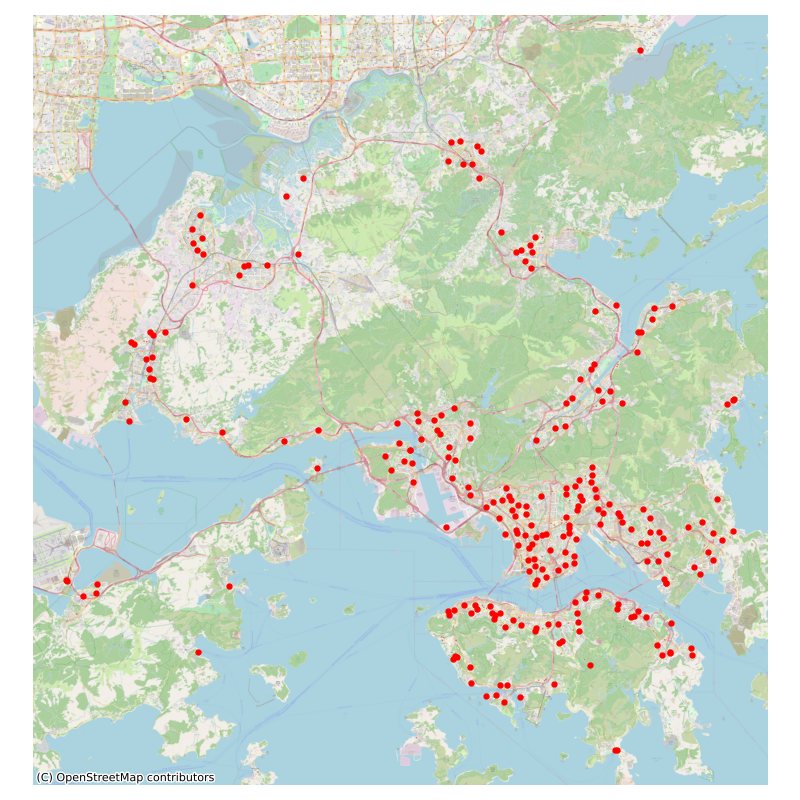
Figure 1: Customer locations

We preprocess the geographic data from the Google Maps API and the Elevation API into the $\alpha$, $\beta$, and $\gamma$ values associated on the arcs (defined in Section 3), so that the proposed solution approaches can compute the fuel consumption and $\text{CO}_{2}e$ emission efficiently. To begin with, for every distinct pair of the stores, we obtain a suggested path by using the Google Maps API and find out the elevation for all the coordinates along the suggested path by using Google Elevation API. Afterward, to construct arc segments, coordinates along a path are divided into segments, with each segment the distance is no longer than 1,000 meters. An arc segment can be viewed as a slope along the suggested path. In our experiments, there are in total 155,333 such slopes. Lastly, the angles and distance of all these slopes are determined using the coordinates and elevation data, and thus we have the $\alpha$, $\beta$, and $\gamma$ values of all the arcs connecting the stores.

In our experiments, nine instances are constructed. Each instance consists of 100 customers which are randomly selected amongst the 248 stores. The ready time, due time, demand, vehicle number, and capacity are data from the Solomon’s C class instances. The depot is located at the Kwai Tsing Container Terminal which is the busiest port in Hong Kong.

6.3 Parameter tuning

The best parameters amongst the values specified in Table 6 are chosen for each instance class.

Table 6: Parameter Values

Parameter	Possible values	Description
$I_{1}$	1, 2	Number of iterations in the first phase
$I_{2}$	100,000	Number of iterations in the second phase
$\lambda$	$10^{-6}$, $5\times 10^{-6}$, $10^{-7}$, $5\times 10^{-7}$	Diversification intensity
$h$	3, 4, 5, 6	Parameter for setting the tabu tenure
$\delta$	10, 20, 30, 40	Penalty update frequency

All experiments have been conducted on a server computer running Ubuntu with an Intel Xeon CPU E5-2698 v3 @ 2.30GHz, 16 cores, and 15 GB of main memory. Algorithms have been implemented in C++ and compiled using GNU g++ version 10.2.0 with -O2 flag. The algorithms run on a single core per instance.

6.4 Efficiency of the approaches

Table 7 summarizes the computational results of BP and TS on the instances described in Section 6.1 with 25, 50, 75 and 100 customers respectively. Results on individual instances are shown in Appendix A. Column NI is the number of instances in the dataset class excluding the ones that no feasible solution can be found by using BP within 3 hours. Column NO is the number of instances that can be solved to optimality by using BP within the time limit. Column NV is average number of vehicle routes, column TD is average total travel cost, column AT is the average cpu time (in seconds), and column AG is the average optimality gap (in percentage). When reporting the average values, we excluded the instances that no feasible solution can be found by using BP within 3 hours.

Table 7: Computational Results of the PRP-SO Instances

			BP					TS
Class		NO/NI	NV	TD	AT (s)	AG (%)		NV	TD	AT (s)
N25	C	9/9	3.000	24.059	215.90	0%		3.000	24.597	0.41
	RC	8/8	3.250	45.314	30.28	0%		3.250	45.331	0.98
	R	12/12	4.667	60.240	30.02	0%		4.750	59.306	2.49
N50	C	7/7	5.000	45.641	3608.80	0.000%		5.000	46.612	2.65
	RC	4/8	6.500	94.850	6933.27	0.087%		6.500	97.514	10.26
	R	9/10	7.500	107.889	2707.29	0.018%		8.000	109.131	8.17
N75	C	2/4	8.000	83.020	8314.54	0.079%		8.000	82.994	3.85
	RC	1/6	9.667	154.001	9262.17	4.088%		10.333	153.598	10.03
	R	5/6	11.833	152.447	3956.78	0.018%		12.500	160.035	8.23
N100	C	1/1	10.000	107.742	3255.73	0.000%		10.000	107.742	2.21
	RC	1/4	12.750	210.165	8957.57	2.440%		13.000	195.959	12.93
	R	2/3	16.667	194.144	4489.88	1.983%		13.500	170.702	42.31
Total:		61/78	98.8	1279.5	51762.2			97.8	1253.5	104.5

As shown in Table 7, BP can solve instances up to 100 customers, with 61 instances (53%) solved to optimality. BP can find all the optimal solutions of the dataset with 25 customers within a reasonable time, and most optimal solutions of the dataset with 50 customers within 3 hours. As compared to TS, BP can determine better solutions on smaller instances, but at the expense of significantly more CPU time. TS can find near-optimal solutions for all instances within one minute, and outperforms BP on solution quality for the dataset with 100 customers.

6.5 The value of using elevation information

For evaluating the potential benefits of using elevation information in optimizing the vehicle routes, the real-world instances described in Section 6.2 are solved by using TS. Table 8 summaries the total distance (in km), average speed (in km/h), total fixed cost (in EUR), total fuel cost (in EUR), and the total elevation (in meters). Figure 2 illustrates an example vehicle route. The same dataset is solved again with which elevation information is ignored when planning the vehicle routes. The results are reported in Table 9. This is achieved in our experiment by setting the angles of all slopes to zero when optimizing the vehicle routes by using TS, and evaluating the solutions with the correct elevations and slopes after the vehicle routes have been decided.

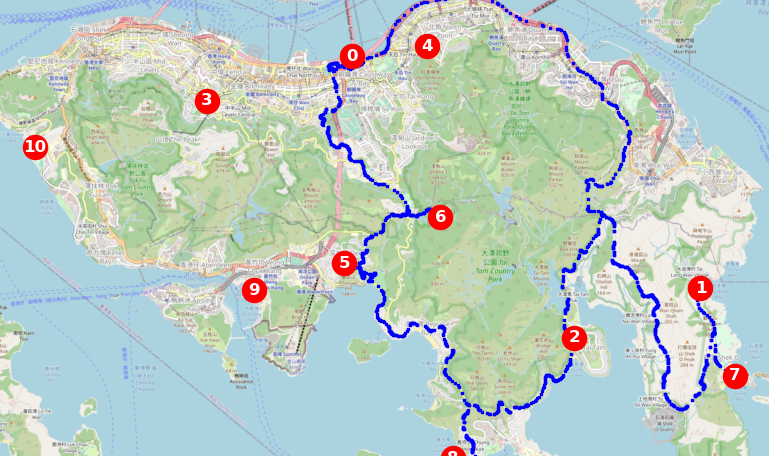
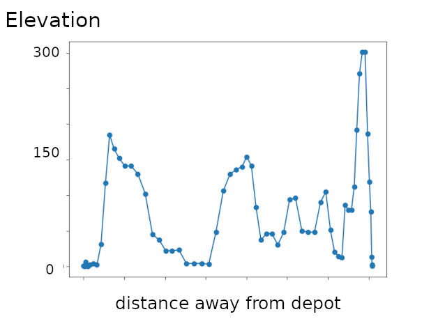
Figure 2: An example vehicle route

Table 8: Results on Real-world Instances

Instance	Distance	Speed	Fixed cost	Fuel cost	Elevation
HK01	1638.6	62.3	1500	109.5	1816
HK02	1460.1	62.3	1400	163.6	1436
HK03	990.2	61.1	1200	196.7	1070
HK04	1153.7	63.1	1000	50.0	1440
HK05	1209.0	63.5	1400	197.5	1185
HK06	1441.9	64.9	1300	89.4	1748
HK07	1159.5	65.5	1300	185.4	1309
HK08	1384.8	64.6	1200	110.3	1359
HK09	1088.5	63.7	1100	81.5	1495
Average:	1280.7	63.5	1266.7	131.5	1428.7

Table 9: Results on Real-world Instances when Slopes are Ignored

Instance	Distance	Speed	Fixed cost	Fuel cost	Elevation
HK01	1158.7	60.6	1500	405.1	1582
HK02	1015.1	60.7	1400	331.1	1152
HK03	953.0	60.9	1200	184.5	1043
HK04	765.2	60.5	1100	114.5	1443
HK05	1040.7	62.9	1400	409.8	1140
HK06	1071.8	62.8	1300	518.3	1536
HK07	1004.4	62.3	1300	278.1	1311
HK08	945.3	64.0	1300	197.7	1307
HK09	831.7	59.5	1100	138.0	1331
Average:	976.2	61.6	1288.9	286.3	1316.1

We can observe the impacts on solutions when elevation information is used for planning the vehicle routes by comparing the results in Table 8 and Table 9. As shown in the experimental results, when elevation information is considered in planning, fuel consumption decreased by 54% on average while the average vehicle speed and elevation increased slightly, and the total travel distance increased by 31%. Larger travel distances and lower fuel consumption seem to be contradictory for typical vehicle routing problems. This is because differs from typical vehicle routing problems, the fuel consumption now depends not only on the distance, but also on the slopes, payload, and vehicle speeds. Optimal vehicle routes should therefore save fuel costs by avoiding going uphill at a high speed with a large payload. As a result, vehicles tend to visit more customers first before going uphill. Although this will increase travel distance, fuel consumption can be saved from going uphill with less payload.

For typical vehicle routing problems or when vehicle routes are planned manually, travel distance is usually minimized in the objective function. Our experimental result reveals that this can lead to a suboptimal solution in reality. With the elevation information, the optimal solution can balance the tradeoff between the energy consumption due to longer distances and the higher payload when going uphill. To avoid high fuel consumption when vehicles going uphill, heavier items tend to be delivered first before going uphill. Customer time windows have to be taken into account so that vehicles do not need to speed up to meet the due times which can result in high fuel consumption. If elevation information is ignored when planning the vehicle routes, fuel consumption due to payload is underestimated when vehicles are going uphill, which leads to poor solutions. With the significant savings we observed from the experimental results, logistic service providers should consider using elevation data for planning their vehicle routes in practice.

6.6 Impact of payloads and slopes

For evaluating the impact of payloads and slopes on the optimized solutions, the real-world instances described in Section 6.2 are modified by scaling the payloads by a factor $r_{1}\in\{0,0.1,...,1\}$ when calculating the costs, and scaling the slopes by a factor $r_{2}\in\{0,0.1,...,1\}$. In our experiments, we replace the payload $x_{ke}$ in (1) by a factor $r_{1}x_{ke}$ when calculating the costs, and replace the slope $\phi_{es}$ in (3) by $r_{2}\phi_{es}$ when preprocessing the data. A higher value of the payload factor ($r_{1}$) represents scenarios when relatively heavier items are shipped, and a higher value of the slope factor ($r_{2}$) represents more hilly areas where steep slopes commonly appear. There are 1089 instances tested in total, and each of them is solved by using TS with a timelimit of 300 seconds. Table 10 summarizes the average costs (and refer to appendix B for the complete results). Figure 3 shows the average cost with varying payloads ($r_{1}$) and slopes ($r_{2}$) respectively.

Table 10: Impact of Payloads and Slopes on Routing Costs

		Slope factor ($r_{2}$)
		0	0.2	0.4	0.6	0.8	1	Average
Payload factor ($r_{1}$)	0	1516.0	1543.9	1527.4	1458.7	1456.2	1361.8	1477.3
	0.2	1514.3	1519.5	1527.3	1472.0	1475.4	1374.8	1480.6
	0.4	1530.7	1563.0	1540.4	1466.4	1478.4	1363.9	1490.5
	0.6	1545.9	1565.5	1556.6	1475.9	1512.0	1373.8	1505.0
	0.8	1553.0	1532.5	1582.0	1511.1	1494.6	1404.7	1513.0
	1	1575.1	1542.8	1586.7	1516.6	1496.1	1413.3	1521.8
	Average	1539.2	1544.6	1553.4	1483.5	1485.5	1382.0

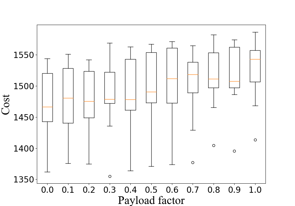
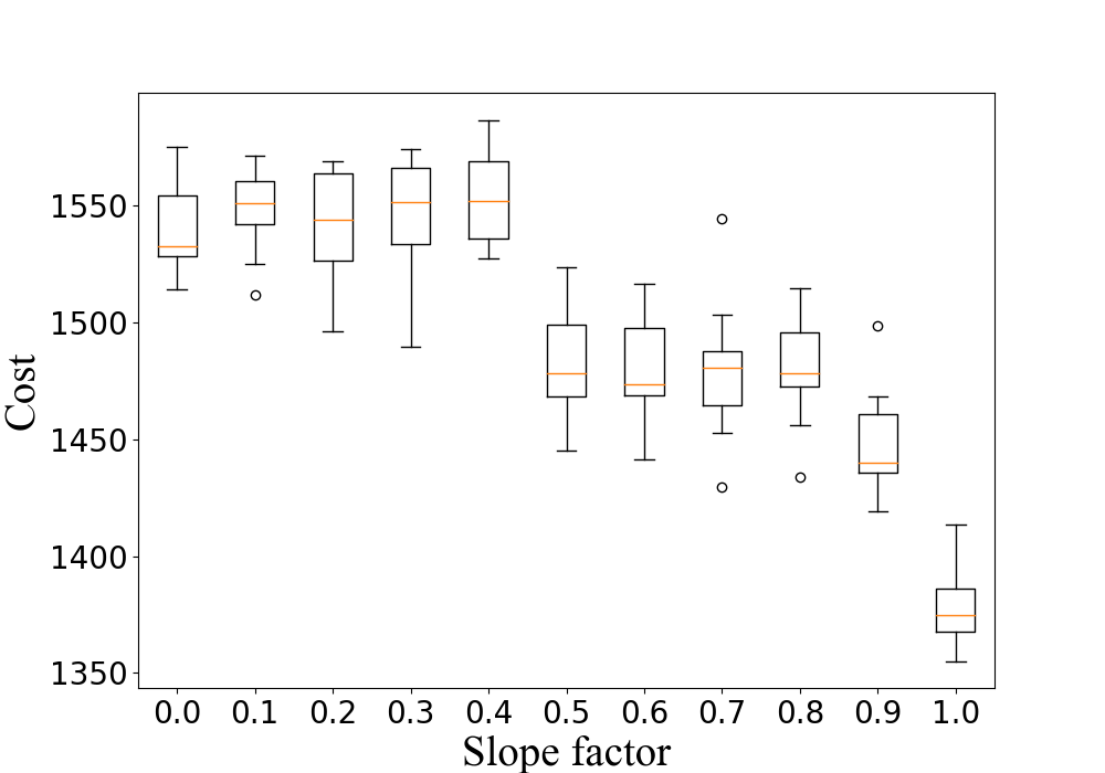
Figure 3: Impact of payloads and slopes on routing costs

From the experimental results, we can see that the shipping cost increases with the payload ($r_{1}$) and decreases with the slope ($r_{2}$). It is more costly to ship with a heavier payload (higher value of $r_{1}$) with a percentage increase in total costs up to 3.49% on average regardless of the slopes. It is less costly to ship in more hilly areas (higher value of $r_{2}$) with a saving up to 11.71% of the total costs on average regardless of the payloads. The impact due to slopes is significantly higher than the impact due to payloads, which reveals the importance of taking into account slopes when optimizing the vehicle routes.

7 Conclusions

This paper formulates and proposes efficient solution methods for a joint Pollution Routing and Speed Optimization Problem (PRP-SO), where the total travel cost is a function of fuel consumption and $\text{CO}_{2}e$ emissions and depends, simultaneously, on road grades, arc payloads, and vehicle speed. The introduction of the vehicle speed as continuous decision variables results in more complicated optimization subproblems in the presence of time window constraints. For the fixed-sequence speed optimization problem where the vehicle route is known, the proposed approach is conceptually simple and computes the optimal vehicle speed (with and without time windows) in quadratic time. In the speed optimization with variable routes, we introduced a novel labeling algorithm, without full backtracking searching, that efficiently determines the cost of a vehicle route that travels with optimal speed. Based on the proposed speed optimization algorithms, we present two general solution approaches for solving the PRP-SO. An approximate solution strategy aims to solve large instances in a short computational time. For this purpose, we integrated the fixed-sequence speed optimization algorithm in a tabu search metaheuristic. The second approach consists of an exact branch-and-price algorithm, in which the variable-route speed optimization is managed within the pricing problem.

We carried out extensive computational experiments on modified Solomon benchmarks and newly constructed real-life instances. Numerical results show that the exact solution methodology performs very well in terms of solution quality: 61 out of 116 instances are solved to optimality. Contrary to the computational outcomes presented by Dabia et al. (2017), in which several instances with only 25 customers cannot be solved, we are able to solve all small-scale problem instances (25 customers) within a reasonable time. Our BP algorithm solved most of the problem instances with 50 customers and reached optimal solutions for some larger benchmark instances with up to 100 customers. We show that our metaheuristic works very effectively for all instances solved. The heuristic consumes less than one minute to find near-optimal solutions in all instances and improved best-known solutions where the exact algorithm did not reach optimality.

Our computational results on real-world instances provide sufficient evidence to suggest some essential managerial insights. First, significant savings (53%) in fuel consumption and $\text{CO}_{2}e$ emissions are observed, especially when shipping heavy items in hilly areas. Second, vehicle routes included a larger number of customer visits (located at flatter terrain) before going to uphill destinations, also significantly reducing fuel consumption. Third, if elevation information is ignored when planning vehicle routes, fuel consumption estimation is inaccurate.

Finally, we do believe that pending issues are requiring future research. From a modeling perspective, the route security (uphill and downhill paths) in hilly topographic cities is a challenging issue to be included. Future studies can now be focused on generalizing the proposed methodological approaches to a new setting where two metrics of performance, fuel consumption, and vehicle route security should be optimized.

Appendix A Results

Table 11: Results on dataset A with 25 customers

	TS			BP
Instance	NV	TD	Time(s)	NV	TD	Time(s)	Gap
c101	3	24.426	0.04	3	24.426	34.48	0.00%
c102	3	23.836	0.33	3	23.278	167.03	0.00%
c103	3	25.120	0.15	3	24.749	564.82	0.00%
c104	3	25.835	0.15	3	23.994	750.72	0.00%
c105	3	23.893	0.04	3	23.893	37.14	0.00%
c106	3	22.743	0.04	3	22.743	30.45	0.00%
c107	3	24.087	0.08	3	24.087	49.42	0.00%
c108	3	25.666	1.10	3	25.199	86.84	0.00%
c109	3	25.767	1.71	3	24.163	222.18	0.00%
r101	8	75.787	0.17	8	75.787	3.43	0.00%
r102	7	67.899	0.25	7	67.899	8.99	0.00%
r103	4	60.948	25.69	4	60.948	20.41	0.00%
r104	4	51.749	0.13	4	51.749	24.55	0.00%
r105	5	73.139	2.24	5	71.878	12.81	0.00%
r106	5	59.079	0.61	4	71.543	17.33	0.00%
r107	4	52.313	0.08	4	52.313	39.68	0.00%
r108	4	50.755	0.14	4	50.755	112.96	0.00%
r109	4	58.009	0.13	4	58.009	17.49	0.00%
r110	4	56.352	0.06	4	56.352	31.29	0.00%
r111	4	55.261	0.14	4	55.261	29.14	0.00%
r112	4	50.382	0.29	4	50.382	42.16	0.00%
rc101	4	59.050	0.36	4	59.050	21.24	0.00%
rc102	3	46.660	0.04	3	46.660	18.98	0.00%
rc103	3	43.835	0.81	3	43.752	38.84	0.00%
rc104	3	40.023	0.51	3	40.023	53.76	0.00%
rc105	4	51.685	0.55	4	51.685	12.62	0.00%
rc106	3	43.845	1.09	3	43.845	17.57	0.00%
rc107	3	39.803	3.75	3	39.803	28.56	0.00%
rc108	3	37.749	0.70	3	37.693	50.68	0.00%

Table 12: Results on dataset A with 50 customers

	TS			BP
Instance	NV	TD	Time(s)	NV	TD	Time(s)	Gap
c101	5	46.632	0.58	5	46.632	355.82	0.00%
c102	5	44.457	1.41	5	44.324	9896.23	0.00%
c105	5	45.762	3.34	5	45.762	1373.90	0.00%
c106	5	43.440	3.14	5	43.440	1014.27	0.00%
c107	5	45.942	1.45	5	45.942	1515.75	0.00%
c108	5	49.758	5.09	5	48.022	4114.59	0.00%
c109	5	50.292	3.51	5	45.368	6991.02	0.00%
r101	11	153.622	40.54	11	136.449	66.09	0.00%
r102	10	118.659	1.68	10	116.500	113.91	0.00%
r103	8	109.075	9.20	8	100.962	352.12	0.00%
r105	9	121.023	1.92	8	128.679	356.35	0.00%
r106	8	105.068	5.83	7	110.509	646.84	0.00%
r107	7	92.989	10.15	6	94.761	3521.55	0.00%
r109	7	113.663	6.36	7	102.349	329.25	0.00%
r110	7	94.271	3.59	6	102.664	2792.51	0.00%
r111	7	95.106	2.04	6	100.870	8357.22	0.00%
r112	6	87.839	0.36	6	85.143	10537.02	0.18%
rc101	8	122.350	8.16	8	120.475	2761.42	0.00%
rc102	7	112.088	21.62	7	108.434	10785.42	0.27%
rc103	6	95.953	9.52	6	92.720	10772.43	0.22%
rc104	5	73.271	19.88	5	71.435	2075.18	0.00%
rc105	8	110.736	8.75	8	108.016	5045.61	0.00%
rc106	6	96.262	3.35	6	94.017	10794.97	0.17%
rc107	6	89.167	3.20	6	85.984	10736.23	0.04%
rc108	6	80.282	7.58	6	77.722	2494.94	0.00%

Table 13: Results on dataset A with 75 customers

	TS			BP
Instance	NV	TD	Time(s)	NV	TD	Time(s)	Gap
c101	8	84.075	1.28	8	84.075	1307.64	0.00%
c105	8	83.800	10.61	8	83.675	10707.30	0.00%
c106	8	80.379	0.60	8	80.743	10524.12	0.26%
c107	8	83.723	2.90	8	83.588	10719.11	0.06%
r101	16	188.867	1.50	16	178.963	239.79	0.00%
r102	14	172.323	1.73	14	164.139	481.14	0.00%
r103	11	146.177	19.15	11	134.750	5015.91	0.00%
r105	12	174.159	8.76	11	154.253	744.75	0.00%
r106	11	146.746	8.86	10	147.330	10769.54	0.11%
r109	11	131.937	9.36	9	135.247	6489.55	0.00%
rc101	12	182.652	1.26	12	176.597	2595.03	0.00%
rc102	11	171.448	18.98	10	168.386	10771.39	0.10%
rc103	10	143.512	0.63	9	146.403	10539.07	0.84%
rc106	11	153.381	3.68	9	158.384	10750.79	0.20%
rc107	9	144.181	33.79	9	144.269	10772.05	10.87%
rc108	9	126.413	1.85	9	129.969	10144.71	12.52%

Table 14: Results on dataset A with 100 customers

	TS			BP
Instance	NV	TD	Time(s)	NV	TD	Time(s)	Gap
c101	10	107.742	2.21	10	107.742	3255.73	0.00%
r101	20	211.371	6.76	19	207.751	983.72	0.00%
r102	18	206.003	18.26	17	190.955	2111.25	0.00%
r105	15	186.240	7.66	14	183.726	10374.66	5.95%
rc101	16	225.632	5.18	14	224.172	10786.57	0.22%
rc102	14	209.526	13.02	12	221.372	10585.25	1.80%
rc105	15	245.247	24.93	13	211.847	3935.69	0.00%
rc106	13	195.968	22.91	12	183.270	10522.80	7.75%

Appendix B Impact of Payloads and Slopes on Routing Costs

Table 15: Impact of Payloads and Slopes on Routing Costs

Slope factor ($r_{2}$) 0.0 0.1 0.2 0.3 0.4 0.5 0.6 0.7 0.8 0.9 1.0 Average Payload factor ($r_{1}$) 0.0 1516.0 1525.0 1543.9 1490.0 1527.4 1466.6 1458.7 1429.5 1456.2 1419.1 1361.8 1472.2 0.1 1525.6 1550.8 1496.3 1530.8 1536.9 1455.9 1441.2 1480.4 1433.8 1439.8 1375.7 1478.8 0.2 1514.3 1542.1 1519.5 1536.1 1527.3 1445.3 1472.0 1452.6 1475.4 1445.6 1374.8 1482.3 0.3 1532.6 1511.8 1564.2 1489.7 1569.1 1478.0 1473.6 1478.8 1470.4 1435.7 1355.1 1487.2 0.4 1530.7 1545.8 1563.0 1551.3 1540.4 1474.5 1466.4 1454.4 1478.4 1455.9 1363.9 1493.2 0.5 1530.8 1567.3 1555.8 1567.1 1551.9 1490.6 1470.8 1482.0 1474.8 1439.2 1371.1 1500.1 0.6 1545.9 1571.4 1565.5 1570.8 1556.6 1470.0 1475.9 1475.0 1512.0 1435.6 1373.8 1504.8 0.7 1562.1 1541.6 1520.5 1564.9 1534.8 1518.6 1488.3 1489.5 1514.7 1429.3 1377.1 1503.8 0.8 1553.0 1553.9 1532.5 1564.9 1582.0 1499.2 1511.1 1503.4 1494.6 1465.7 1404.7 1515.0 0.9 1555.6 1552.7 1568.9 1574.3 1569.3 1498.9 1507.3 1486.3 1495.6 1498.7 1395.3 1518.4 1.0 1575.1 1569.9 1542.8 1543.2 1586.7 1523.5 1516.6 1544.5 1496.1 1468.2 1413.3 1525.4 Average 1540.1 1548.4 1543.0 1543.9 1553.0 1483.7 1480.2 1479.7 1482.0 1448.4 1378.8

References

- Bandeira et al. (2013) J. Bandeira, T. G. Almeida, A. J. Khattak, N. M. Rouphail, and M. C. Coelho. Generating emissions information for route selection: Experimental monitoring and routes characterization. Journal of Intelligent Transportation Systems, 17(1):3–17, 2013.
- Barth and Boriboonsomsin (2009) M. Barth and K. Boriboonsomsin. Energy and emissions impacts of a freeway-based dynamic eco-driving system. Transportation Research Part D: Transport and Environment, 14(6):400–410, 2009.