Energy derivatives in real–space diffusion Monte Carlo

Abstract

We present unbiased, finite–variance estimators of energy derivatives for real–space diffusion Monte Carlo calculations within the fixed–node approximation. The derivative $d_{\lambda}E$ is fully consistent with the dependence $E(\lambda)$ of the energy computed with the same time step. We address the issue of the divergent variance of derivatives related to variations of the nodes of the wave function, both by using a regularization for wave function parameter gradients recently proposed in variational Monte Carlo, and by introducing a regularization based on a coordinate transformation. The essence of the divergent variance problem is distilled into a particle-in-a-box toy model, where we demonstrate the algorithm.

I Introduction

Variational Monte Carlo (VMC) and diffusion Monte Carlo (DMC) are numerical stochastic approaches based on a real–space representation of a correlated trial wave function to study many–body quantum systems, including electronic structure problems. VMC calculates expectation values of quantum operators on the trial function, which in turn is optimized via minimization of a suitable cost function such as the variational energy. DMC further improves the VMC results through a stochastic implementation of the power method, which projects the lowest–energy component of the trial function. Its accuracy, in the fixed–node (FN) approximation almost invariably adopted to avoid the sign problem, is ultimately limited by the error in the nodal surface of the trial function. Martin et al. (2016)

In the last decade, the efficient calculation of analytic energy derivatives, Sorella and Capriotti (2010); Filippi et al. (2016) leveraging modern optimization methods, Umrigar et al. (2007); Toulouse and Umrigar (2007); Sorella et al. (2007) spawned impressive progress in both accuracy and scope of the VMC method. Kent et al. (2020); Nakano et al. (2020); Needs et al. (2020); Feldt and Filippi (2020)

DMC largely benefits from advances in VMC because improved trial functions tend to have better nodes. However, it would be desirable to have efficient and unbiased estimators of derivatives in DMC as well, to perform such tasks as the direct optimization of the nodal surface or DMC structural relaxation. This is still an open issue, with the latest developments featuring uncontrolled approximations and/or very low efficiency Badinski et al. (2010); Assaraf et al. (2011); Moroni et al. (2014). Here we present an algorithm to calculate unbiased energy derivatives in FN–DMC with finite variance.

II Energy derivatives

In both VMC and DMC, the energy is calculated as

$$E=\int P(R)E_{L}(R)dR\bigg{/}\int P(R)dR\equiv\Big{\langle}E_{L}\Big{\rangle}_{P}$$ (1)

where $R$ represents the coordinates of all the particles, $E_{L}(R)=H\Psi(R)\big{/}\Psi(R)$ is the local energy of the trial function $\Psi(R)$, and $P(R)$ is proportional to the underlying probability distribution: in VMC, $P(R)=\Psi^{2}(R)$, and, in DMC, $P(R)=\Psi(R)\Phi(R)$ with $\Phi(R)$ the FN solution. The derivative with respect to a parameter $\lambda$ is

$$d_{\lambda}E=\Big{\langle}d_{\lambda}E_{L}+(E_{L}-E)d_{\lambda}\ln P\Big{\rangle}_{P}$$ (2)

The variance of this naïve estimator is zero if both $\Psi$ and its derivative $d_{\lambda}\Psi$ are exact; however, for an approximate trial function, $E_{L}(R)$ diverges at the nodes as $1\big{/}d(R)$, where $d=|\Psi|\big{/}\left\|\nabla\Psi\right\|$, and the variance diverges as well. Attaccalite and Sorella (2008); Pathak and Wagner (2020)

II.1 Regularized estimators

In VMC, this problem was fully solved by Attaccalite and Sorella Attaccalite and Sorella (2008) with a reweighting scheme, hereafter dubbed AS, whereby one samples the square of a modified trial function ${\widetilde{\Psi}}$ which differs from $\Psi$ only for $d$ smaller than a cutoff parameter $\epsilon$ and stays finite on the nodal surface of $\Psi$. A similar sampling scheme was proposed by Trail Trail (2008a). The AS estimator has the same average of the bare estimator of eq 2  for any value of $\epsilon$, and finite variance.

An alternative regularized estimator, recently proposed by Pathak and Wagner, Pathak and Wagner (2020) simply consists in multiplying the term in brackets of eq 2  by the polynomial $f_{\epsilon}(x)=7x^{6}-15x^{4}+9x^{2}$, with $x=d\big{/}\epsilon$, whenever $x<1$. This estimator, hereafter dubbed PW, has finite variance for any finite $\epsilon$ and a bias which vanishes as $\epsilon\to 0$. The polynomial is chosen in such a way to remove from the bias the linear term, shown Pathak and Wagner (2020) to be $\propto\int_{0}^{1}(f_{\epsilon}-1)dx$, and to be continuously differentiable in $(0,1)$. The odd parity of fermionic wave functions near a node then implies a cubic leading term in the bias. Since various values of $\epsilon$ can be used in the same simulation, the bias can be eliminated at no cost by extrapolation. The PW estimator has been proposed for parameter gradients in the VMC optimization of $\Psi$, but it is equally applicable to VMC interatomic forces and, as we will show, to generic derivatives in DMC.

We introduce a third regularized estimator, that we denote “warp” by analogy with the space–warp transformation of ref. 17  devised to reduce the statistical noise of the forces. There, as a nucleus is displaced, a transformation is applied to the coordinates of nearby electrons, in such a way to maintain the electron–nucleus distances approximately constant. Here, the goal is to maintain constant the value of $d(R)$ when the nodal surface is displaced by a variation of the parameter $\lambda$. In this way, the diverging term in the local energy does not change, and the variance of the derivative is finite.

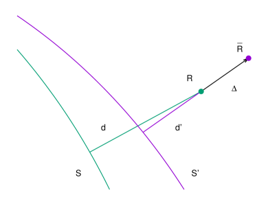
Figure 1: Schematic picture of the warp transformation. The curve $S$ is the nodal surface for the value $\lambda_{0}$ of the parameter $\lambda$. The value of $d$ for the current configuration $R$ is pictorially represented as the distance from $S$ (this is strictly true only if $\Psi$ is linear, i.e. close enough to the node). When a variation of $\lambda$ from $\lambda_{0}$ to $\lambda^{\prime}$ shifts $S$ to $S^{\prime}$, the value of $d$ changes to $d^{\prime}$. Hence, we displace $R$ by an amount $\Delta=d-d^{\prime}$ to $\overline{R}$ in the direction of ${\rm sign}(\Psi^{\prime})\nabla\Psi^{\prime}(R)$, so that the value of $|\Psi^{\prime}(\overline{R})|\big{/}\left\|\nabla\Psi^{\prime}(\overline{R})\right\|$ is approximately equal to $d$.

The warp transformation, illustrated in Figure 1 , is defined as

$$\overline{R}=R+\left[d(R)-d^{\prime}(R)\right]{\rm sign}\left(\Psi^{\prime}(R)\right)n^{\prime}(R)u(d(R))$$ (3)

where primed quantities are calculated for the value $\lambda^{\prime}$ of the parameter, $n^{\prime}$ is the unit vector in the direction of $\nabla\Psi^{\prime}(R)$, and $u(d)$ is a cutoff function with support $[0,\epsilon]$ which decreases smoothly from 1 to 0, restricting the warp transformation to a region close to the nodal surface. We use the quintic polynomial with zero first and second derivatives at the boundaries of the support.

For a finite increment of $\lambda$, the energy is

$$E^{\prime}=\int E^{\prime}_{L}(\overline{R})P^{\prime}(\overline{R})JdR\bigg{/}\int P^{\prime}(\overline{R})JdR,$$ (4)

where $J=\det J_{ij}=\det\partial\overline{R}_{i}\big{/}\partial R_{j}$ is the Jacobian of the transformation. The analytic derivative $d_{\lambda}E$, calculated at the value of the parameter $\lambda=\lambda_{0}$, is:

$$d_{\lambda}E\big{|}_{\lambda_{0}}=\Big{\langle}\partial_{\lambda}E_{L}+\nabla E_{L}\cdot\partial_{\lambda}\overline{R}$$

$$+(E_{L}-E)\left[\partial_{\lambda}\ln(PJ)+\nabla\ln P\cdot\partial_{\lambda}\overline{R}\right]\Big{\rangle}_{P}$$ (5)

This warp regularized estimator has finite variance and no bias for any value of $\epsilon$.

Note that all the functions in eq 5  are evaluated at $\lambda=\lambda_{0}$, where $\overline{R}=R$ and $J=1$. Therefore the warp transformation only contributes to the estimator, through the derivatives $\partial_{\lambda}\overline{R}_{i}\big{|}_{\lambda_{0}}$ and $\partial_{\lambda}\ln J\big{|}_{\lambda_{0}}$, while the sampling is done over one and the same distribution $P(R)$ for any parameter we may vary.

Furthermore, for $\lambda=\lambda_{0}$, the cofactors of the Jacobi matrix $J_{ij}$ are $M_{ij}=\delta_{ij}$, and the seemingly awkward derivative of the Jacobian greatly simplifies, $\partial_{\lambda}\ln J\big{|}_{\lambda_{0}}=\sum_{ij}M_{ij}\partial_{\lambda}J_{ij}\big{|}_{\lambda_{0}}=\sum_{i}\partial_{\lambda}J_{ii}\big{|}_{\lambda_{0}}$, so that the implementation of eq 5  is not overly complicated. In particular, most of the derivatives needed are already present –or very similar to those already present– in VMC codes with analytic derivatives for structural and full variational optimization. The only exceptions are the off–diagonal components of the the Hessian $\partial^{2}\Psi/\partial R_{i}\partial R_{j}$ and their derivatives with respect to $\lambda$, which contribute to $\partial_{\lambda}J$. We will show (heuristically) that the bias incurred by neglecting those terms can be extrapolated out at no cost.

II.2 Variational Monte Carlo

Before addressing the derivatives in DMC, we compare the three regularized estimators PW, AS, and warp in VMC. To this purpose, it is expedient to consider a system stripped of all complexities of external and interparticle potentials, so that we can focus exclusively on the divergence of the local energy at the nodal surface. Our toy model is a free particle in an elliptic box with hard walls, meant to represent the configuration of a generic system within a nodal pocket. Atomic units are used throughout. We choose $\Psi=\Psi_{0}(x,y)=a^{2}-x^{2}\big{/}C-y^{2}\big{/}(C-1)$ with $C=[\cosh(1)]^{2}=2.3810978$, which is positive inside the ellipse, vanishes at the border, and is not the true ground state. Therefore, the ellipse is defined through the wave function, and we take the derivative with respect to the parameter $a$, which changes the size of the ellipse at constant eccentricity.

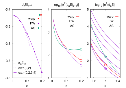
Figure 2: VMC calculations of $d_{a}E$, with integrals performed by quadrature. Left panel: the derivative at $a=1$ obtained with the warp, PW, and AS estimators as a function of the cutoff $\epsilon$, compared to the “exact” result $d_{a}E_{\rm fit}$, defined as the derivative of a fit to $E(a)$ calculated separately for several values of $a$. AS and warp, shown here only near $\epsilon=0.2$, are unbiased; PW can be extrapolated to the unbiased result either including only the leading term in $\epsilon$, here $\epsilon^{2}$, on a sufficiently small range (dashed line) or using a sufficiently large number of terms on an extended range (solid line). Middle panel: variance (in logarithmic scale) of the various regularized estimators as a function of the cutoff. As $\epsilon$ vanishes, all schemes regress to the infinite variance of the bare estimator. Right panel: variance (in logarithmic scale) of the various regularized estimators as a function of the parameter $a$. For the warp and AS estimators, $\epsilon=0.2$; for PW, data are reported for $\epsilon=0.0125$, 0.025, 0.05, 0.15 and 0.2 in order of decreasing variance. Common data in the middle and the right panels are circled.

The average and variance of the various estimators, calculated by quadrature, are shown in Figure 2 . None of the regularized estimators entails uncontrolled approximations. In particular, although there is no rigorous way to establish the range where the leading correction in $\epsilon$ is sufficient, or the number of powers in $\epsilon$ needed over an arbitrary range, PW can be accurately extrapolated to the unbiased result. Here, the bias of the PW estimator has a leading contribution of $\epsilon^{2}$ because $\Psi_{0}$ does not have odd parity across the node. The second–order bias can be removed with a different choice of the polynomial, e.g. $f_{\epsilon}(x)=60x^{2}-200x^{3}+225x^{4}-84x^{5}$. Here, we stick with the original estimator of ref. 15 , but we note that there is a freedom in the choice of $f_{\epsilon}$ that can be tailored for optimal performance in specific situations. The right panel shows that the relative efficiency may depend on the system at hand; in this example, it varies over the range of $a$ considered.

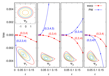
Figure 3: Bias of the VMC derivative for PW and warp with approximate Hessian, calculated by quadrature for various wave functions $\Psi_{1}$–$\Psi_{4}$. In each case, we show a contour plot of the normalized $\Psi_{i}$ with level lines from 0 in steps of 0.2 (the contour plot of $\Psi_{0}$ in the top left inset defines the $(x,y)$ scale). The colored labels near each curve indicate the powers in $\epsilon$ needed to extrapolate to the unbiased value with five–digit accuracy. The bias of PW for $\Psi_{2}$–$\Psi_{4}$ has a leading term $\epsilon^{3}$ because of the odd parity of the wave function across the relevant node. Empirically we see that the warp estimator has a cubic leading term in all cases, including $\Psi_{1}$.

The bias of the warp estimator when the off–diagonal elements of the Hessian are neglected is compared to the bias of the PW estimator in Figure 3 . Since we need a non–diagonal Hessian to start with, we consider (i) a rotated, more eccentric ellipse with a further non–symmetrical distortion of the wave function, and (ii–iv) the positive lobe of a wave function limited to half of the original ellipse by the nodal line $y+\sin(\alpha x)=0$, with $\alpha=0.5$, 1 and 1.5 (see the contour plots in Figure 3 ). The derivative is taken with respect to $a$ for $\Psi_{1}$, and with respect to $\alpha$ for $\Psi_{2}$–$\Psi_{4}$. Within this (very limited) set of test cases, the bias is smaller and less system–dependent for the warp than for the PW estimator. The important result is that neither involves uncontrolled approximations, as both can be extrapolated to the unbiased result in a single run. We have also verified that the warp estimator with the full Hessian is unbiased for finite $\epsilon$.

II.3 Diffusion Monte Carlo

We now consider the derivative in DMC. The FN–DMC algorithm is a branching random walk of many weighted walkers, generated by a short–time approximation $G(R^{\prime},R)$ to the importance–sampled Green’s function, which asymptotically samples the distribution $P(R)=\Psi(R)\Phi(R)$. Martin et al. (2016) The problem with the derivative estimator, eq 2 , is the presence of the logarithmic derivative of $P(R)$, which is not a known function of $R$. However, $P$ is the marginal distribution of the joint probability density $P_{\rm joint}$ of the whole random walk, which does have an explicit expression as a product of Green’s functions,

$$P(R_{n})=\int dR_{0}\ldots dR_{n-1}P_{\rm joint}(R_{n},R_{n-1}\ldots,R_{0})$$

$$\equiv\int dR_{0}\ldots dR_{n-1}\prod_{i=0}^{n-1}G(R_{i+1},R_{i})P_{0}(R_{0})$$ (6)

where $P_{0}$ is the (largely arbitrary) probability distribution of the initial configuration $R_{0}$. Therefore, it is sufficient to consider the estimator of $d_{\lambda}E$ in eq 2  as an average over the whole trajectory of the random walk, rather than over the current configuration, to bring an explicitly known probability distribution to the fore. Moroni et al. (2014) This is similar to the calculation of forces in path integral Monte Carlo. Zong and Ceperley (1998)

In practice, the inclusion of the entire trajectory in the estimator is not necessary. As shown in ref. 13 . the logarithmic derivative of the DMC density distribution $P$ in the estimator of eq 2  can be replaced by the summation

$$d_{\lambda}\ln P(R_{n})=d_{\lambda}\sum_{i=n-k}^{n-1}\ln G(R_{i}^{\prime},R_{i})$$ (7)

over the last $k$ steps of the random walk, with $R_{n}$ the current configuration $R$ of eq 2 . The omitted term, Moroni et al. (2014) $\big{\langle}\left[E_{L}(R_{n})-E\right]d_{\lambda}\ln P(R_{n-k})\big{\rangle}$, vanishes for sufficiently large $k$ because $E_{L}(R_{n})$ and $d_{\lambda}\ln P(R_{n-k})$ become statistically independent variables and $\big{\langle}E_{L}-E\big{\rangle}=0$.

In eq 7 , $G(R_{i}^{\prime},R_{i})$ is the transition rule from $R_{i}$ to $R_{i}^{\prime}$ of the random walk. It includes a Metropolis test to reduce the time step error; Martin et al. (2016) therefore, $R_{i}^{\prime}$ is the configuration proposed when the walker is at $R_{i}$, and the next configuration $R_{i+1}$ is $R_{i}^{\prime}$ or $R_{i}$ if the move is accepted or rejected, respectively. Note that in the formal expression of $P_{\rm joint}$, eq 6 , the arguments of the Green’s functions are integrated over, whereas in the contribution to the estimator of the derivative, eq 7 , they are the particular values of the particles’ coordinates effectively sampled by the random walk. Correspondingly, the actual value taken by $G(R^{\prime},R)$ is

$$\begin{cases}T(R^{\prime},R)p(R^{\prime},R)W(R^{\prime},R)&\text{for an accepted move}\\ T(R^{\prime},R)[1-p(R^{\prime},R)]W(R,R)&\text{for a rejected move}\end{cases}$$ (8)

where $T$ is the a–priori transition probability, $p$ the probability of accepting the move, and $W$ the branching factor (see below).

The inclusion of rejected configurations in eq 7  and of the factor $p$ or $1-p$ in eq 8  in the derivative of the full Green’s function are instrumental to obtain an estimate of $d_{\lambda}E$ completely consistent with the DMC energy $E(\lambda)$ calculated at the same time step. Their omission still can give an unbiased result in the limit $\tau\to 0$, but it may cause an unacceptably large time step error on the derivative. Moroni et al. (2014)

The functions $T$, $p$, and $W$ are standard: Umrigar et al. (1993)

$$T(R^{\prime},R) = \exp\left\{-\left[R^{\prime}-R-F(R)V(R)\tau\right]^{2}/2\tau\right\}$$

$$p(R^{\prime},R) = \begin{cases}0&\text{if the move crosses a node}\\ \min\left\{1,\left[\Psi^{2}(R^{\prime})T(R,R^{\prime})\right]\Big{/}\left[\Psi^{2}(R)T(R^{\prime},R)\right]\right\}&\text{otherwise}\end{cases}$$ (9)

$$W(R^{\prime},R) = \exp\left\{[S(R^{\prime})+S(R)]\tau/2\right\}.$$

Here, $\tau$ is the time step, $V=\nabla\ln\Psi$ is the so–called velocity, and $F(R)=\sqrt{2V^{2}\tau-1}/(V^{2}\tau)$ is the damping factor of its divergence near the nodes; the logarithm of the branching factor is also damped at the nodes, $S(R)=\left[E_{\rm est}-E_{L}(R)\right]F(R)-\ln(N/N_{0})$, where $E_{\rm est}$ is the best current estimate of the energy and $N$ and $N_{0}$ are the current and the target number of walkers.

The presence of $E_{\rm est}$, the Monte Carlo estimate of $E$, in the branching term $S$ implies that the calculation of $d_{\lambda}E$ includes a contribution proportional to $d_{\lambda}E$ itself:

$$\tau\Big{\langle}\sum_{i}[E_{L}(R_{n})-E]F(R_{n-i})\Big{\rangle}d_{\lambda}E\equiv\overline{F}d_{\lambda}E$$ (10)

This does not require prior knowledge of the result: we can calculate the factor $\overline{F}$ and $(d_{\lambda}E)_{0}$, the derivative when the contribution of eq 10  is omitted, and combine them to get the unbiased result as $d_{\lambda}E=(d_{\lambda}E)_{0}+\overline{F}d_{\lambda}E$, or $d_{\lambda}E=(d_{\lambda}E)_{0}/(1-\overline{F})$.

The main technical complication in DMC is the need to store a few quantities for each derivative and for each value of $\epsilon$ over the last $k$ steps of each walker, namely $d_{\lambda}\ln G$ and $E_{L}d_{\lambda}\ln G$ to implement eq 2  with the probability distribution $P$ of eq 7 , and $F$ and $E_{L}F$ to implement eq 10 .

The AS regularized estimator has been applied to approximate DMC forces in refs. 13; 20 . However it pushes a finite density of walkers on the nodes, which is presumably not optimal in DMC. Furthermore, unlike in VMC, it requires Moroni et al. (2014) an extrapolation to $\epsilon\to 0$ which –at difference with the PW and warp estimators– cannot be done in a single run.

Therefore, for the DMC derivatives we consider only the PW and the warp estimators. For the former, we insert eq 7  into eq 2 , and multiply each term of the resulting summation by a polynomial $f_{\epsilon}$ calculated at the appropriate configuration. For the latter, we just insert eq 7  in eq 5 . For the warp estimator, the argument of the Jacobian needs some care: we evaluate $\partial_{\lambda}\ln J$ in the proposed configuration $R^{\prime}$ for both accepted and rejected moves; alternatively, we can include $\partial_{\lambda}\ln J$ only for the accepted moves, provided the warp transformation is not considered in the derivatives at $R^{\prime}$ when the move is rejected.

We present results of DMC simulations with the wave function $\Psi_{0}$, time step $\tau=0.1$, and target number of walkers $N_{0}=100$. We have verified that in the limit $\tau\to 0$ we recover the analytic results Moon and Spencer (1988) for the ground state energy, $E=2q/a^{2}$ with $q=0.825352549$, within a statistical error of less than one part in 10,000. To this level of accuracy, the population control bias Martin et al. (2016) is negligible.

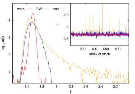
Figure 4: Histogram of 46,000 block averages, each of which taken over 10,000 steps of 100 walkers in a DMC calculation of $d_{a}E\big{|}_{a=1}$. The warp and PW estimators (with $\epsilon=0.2$ and 0.0125, respectively) have nearly Gaussian distributions. The bare estimator has a heavy–tailed distribution; the largest value in the present sample exceeds $x=10$. Inset: the data trace of the first 1,000 block averages.

Figure 4  exposes the drawback of the bare estimator: the probability distribution $p(\xi)$ for the block averages of the derivative features a right heavy tail, consistent with the expected Trail (2008b); Badinski et al. (2010) leading decay $\propto\big{|}\xi-\xi_{0}\big{|}^{-5/2}$. In the data trace, shown in the inset, heavy tails result in large spikes that would mar the smooth convergence of structural or variational optimization. Meaningful averages and statistical uncertainties of heavy–tailed distributions with known tail indices can be computed with a tail regression analysis. López Ríos and Conduit (2019) This technique, however, requires a heavy post–processing not very practical for large–scale applications. The regularized estimators PW and warp, instead, have nearly Gaussian distributions amenable to standard statistical analysis with significantly smaller statistical errors and, most importantly, no large spikes in the data trace.

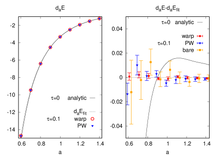
Figure 5: DMC calculations of $d_{a}E$ with $\tau=0.1$. Left panel: the warp and PW results compare favorably with the “exact” result, defined as the derivative $d_{a}E_{\rm fit}$ of a fit to DMC calculations of $E(a)$. The analytic result $d_{a}E=-4q/a^{3}$ differs from $d_{a}E_{\rm fit}$ because the latter has a finite time step error. Right panel: the difference of the calculated derivatives with $d_{a}E_{\rm fit}$ are shown on an expanded scale by subtracting the latter (hence the solid black line is minus the time step error of $d_{a}E_{\rm fit}$). The PW derivatives are extrapolated to $\epsilon\to 0$. We also include the bare–estimator derivatives, with averages and statistical uncertainties obtained with the tail regression estimator analysis toolkit made available in ref. 23 . Small horizontal shifts are applied to same–$a$ data for clarity.

The central result of this work is shown in Figure 5 . We calculate the energy $E$ and its derivative $d_{a}E$ for a set of values of $a$, and compare the DMC derivatives with the derivative of a fit to the DMC energies. All the estimators (bare, extrapolated PW, and warp) are unbiased, which demonstrates the correctness of the proposed algorithm. For comparison, the variational drift–diffusion (VD) approximation of ref. 13  gives for $a=1$ a bias of $\sim 0.2$, twice the full scale of the right panel, and it gets even worse for smaller time steps (although the VD approximation is devised to exploit good wave functions, while our $\Psi_{0}$ is poor on purpose to test the unbiased estimators).

For given $a$, the same run is used for all the estimators. Therefore the statistical error is a direct measure of the square root of their relative efficiency. The statistical errors of the bare, PW, and warp estimators, averaged over the values of $a$ shown in Figure 5 , are in the ratio 4.9:2.4:1. These figures may belittle the PW estimator somewhat, because in this particular example a large quadratic bias needs to be eliminated by extrapolation, but they convey the relevant message that both PW and warp are significantly more efficient than the bare estimator.

Finally, the ratio between the statistical error of the DMC and VMC derivatives calculated with the warp estimator at $\epsilon=0.2$, using the same time step and the same number of Monte Carlo samples, lies between 1.9 and 1.7 in the range of $a$ of Figure 5 . We consider this ratio a favorable indication of the efficiency of the algorithm, which will hopefully spur a full assessment with realistic many–body wave functions.

III Conclusions

In summary, we have presented an algorithm to calculate unbiased, finite–variance derivatives in DMC. The estimate of the derivative with respect to a given parameter is fully consistent with the dependence on that parameter of the FN energy, calculated with the same time step. The tail regression statistical analysis López Ríos and Conduit (2019) can cope with the problem of the infinite variance of the bare estimator. Alternatively, and more efficiently, both the recently proposed PW regularization Pathak and Wagner (2020) and the warp regularization introduced in this work can be used to good effect to eliminate the divergence of the variance.

References

- Martin et al. (2016) R. M. Martin, L. Reining, and D. M. Ceperley, Interacting Electrons (Cambridge University Press, 2016).
- Sorella and Capriotti (2010) S. Sorella and L. Capriotti, J. Chem. Phys. 133, 234111 (2010).
- Filippi et al. (2016) C. Filippi, R. Assaraf, and S. Moroni, J. Chem. Phys. 144, 194105 (2016).
- Umrigar et al. (2007) C. J. Umrigar, J. Toulouse, C. Filippi, S. Sorella, and R. G. Hennig, Phys. Rev. Lett. 98, 110201 (2007).
- Toulouse and Umrigar (2007) J. Toulouse and C. J. Umrigar, J. Chem. Phys. 126, 084102 (2007).
- Sorella et al. (2007) S. Sorella, M. Casula, and D. Rocca, J. Chem. Phys. 127, 014105 (2007).
- Kent et al. (2020) P. R. C. Kent, A. Annaberdiyev, A. Benali, M. C. Bennett, E. J. Landinez Borda, P. Doak, H. Hao, K. D. Jordan, J. T. Krogel, I. Kylänpää, J. Lee, Y. Luo, F. D. Malone, C. A. Melton, L. Mitas, M. A. Morales, E. Neuscamman, F. A. Reboredo, B. Rubenstein, K. Saritas, S. Upadhyay, G. Wang, S. Zhang, and L. Zhao, J. Chem. Phys. 152, 174105 (2020).
- Nakano et al. (2020) K. Nakano, C. Attaccalite, M. Barborini, L. Capriotti, M. Casula, E. Coccia, M. Dagrada, C. Genovese, Y. Luo, G. Mazzola, A. Zen, and S. Sorella, J. Chem. Phys. 152, 204121 (2020).
- Needs et al. (2020) R. J. Needs, M. D. Towler, N. D. Drummond, P. López Ríos, and J. R. Trail, J. Chem. Phys. 152, 154106 (2020).
- Feldt and Filippi (2020) J. Feldt and C. Filippi, “Excited-state calculations with quantum monte carlo,” in Quantum Chemistry and Dynamics of Excited States (John Wiley & Sons, Ltd, 2020) Chap. 8, pp. 247–275.
- Badinski et al. (2010) A. Badinski, P. D. Haynes, J. R. Trail, and R. J. Needs, J. Phys.: Condens. Matter 22, 074202 (2010).
- Assaraf et al. (2011) R. Assaraf, M. Caffarel, and A. C. Kollias, Phys. Rev. Lett. 106, 150601 (2011).
- Moroni et al. (2014) S. Moroni, S. Saccani, and C. Filippi, J. Chem. Theory Comput. 10, 4823 (2014).
- Attaccalite and Sorella (2008) C. Attaccalite and S. Sorella, Phys. Rev. Lett. 100, 114501 (2008).
- Pathak and Wagner (2020) S. Pathak and L. K. Wagner, AIP Advances 10, 085213 (2020).
- Trail (2008a) J. R. Trail, Phys. Rev. E 77, 016703 (2008a).
- Filippi and Umrigar (2000) C. Filippi and C. J. Umrigar, Phys. Rev. B 61, R16291 (2000).
- Zong and Ceperley (1998) F. Zong and D. M. Ceperley, Phys. Rev. E 58, 5123 (1998).
- Umrigar et al. (1993) C. J. Umrigar, M. P. Nightingale, and K. J. Runge, J. Chem. Phys. 99, 2865 (1993).
- Valsson and Filippi (2010) O. Valsson and C. Filippi, J. Chem. Theory Comput. 6, 1275 (2010).
- Moon and Spencer (1988) P. Moon and D. E. Spencer, Field Theory Handbook (Springer, Berlin, Heidelberg, 1988) p. 17 ff.
- Trail (2008b) J. R. Trail, Phys. Rev. E 77, 016704 (2008b).
- López Ríos and Conduit (2019) P. López Ríos and G. J. Conduit, Phys. Rev. E 99, 063312 (2019).