Stationary waves in a superfluid gas of electron-hole pairs in bilayers

Abstract

Stationary waves in the condensate of electron-hole pairs in the $n-p$ bilayer system are studied. The system demonstrates the transition from a uniform (superfluid) to a nonuniform (supersolid) state. The precursor of this transition is the appearance of the roton-type minimum in the collective mode spectrum. Stationary waves occur in the flow of the condensate past an obstacle. It is shown that the roton-type minimum manifests itself in a rather complicated stationary wave pattern with several families of crests which cross one another. It is found that the stationary wave pattern is essentially modified under variation in the density of the condensate and under variation in the flow velocity. It is shown that the pattern is formed in the main part by shortwave modes in the case of a point obstacle. The contribution of longwave modes is clearly visible in the case of a weak extended obstacle, where the stationary wave pattern resembles the ship wave pattern.

I INTRODUCTION

Stationary waves emerge in systems in which the collective mode spectrum is different from the linear one. The well-known example is ship waves on a water surface (see, for instance, [1]). The theory of ship waves was developed by Kelvin. The interest in stationary waves was renewed recently in connection with the study of the superfluidity of atomic Bose-Einstein condensates (BECs). Stationary waves in ⁸⁷Rb BEC were observed in [2] (see also [3]).

The stationary wave pattern reported in [2] is in agreement with the theoretical prediction [4, 5, 6]. It was shown in [4, 5, 6] that stationary waves in the atomic BEC are excited outside the Mach cone. It differs from the case of ship waves on a surface of deep water where waves fill the wedge-shaped region behind the obstacle with the semiangle $\approx 19.5^{\circ}$ [7]. Stationary waves in a two-component atomic BEC were studied in [8, 9]. In two-component condensates the stationary wave pattern is more complicated due to the presence of two Mach cones. In this case the waves are not excited in the intersection of two Mach cones.

The stationary wave pattern similar to [4, 5, 6] emerges in a superfluid gas of exciton polaritons in microcavities [10, 11]. More complicated stationary wave patterns with waves inside the Mach cone occur in the flow past a rigid extended obstacle [12, 13]. Exciton polaritons have very small effective mass (of the order of $10^{-5}$ times the free-electron mass) and due to this the temperature of the transition to the superfluid state can be quite high. The observation of stationary waves in the flow of the condensate past an obstacle with overcritical velocities and the absence of such waves at smaller velocities is considered [14] as a proof for the exciton polariton superfluidity. Due to the smallness of the binding energy of Wannier-Mott excitons in the AlGaAs microcavity in [10], superfluid behavior was observed at $T=5$ K. Later a behavior similar to [10] were observed for Frenkel exciton-polaritons in organic microcavities at room temperature [15].

Exciton polaritons have a finite lifetime and laser pumping is required to support the superfluid state. Spatially-indirect excitons in electron-hole bilayers may have an infinite lifetime. In the high-density limit, these excitons are similar to Cooper pairs in superconductors, and the description of such systems can be given in the framework of a modified version [16, 17, 18, 19, 20] of the Bardin-Cooper-Schrieffer (BCS) theory [21]. In the low-density limit the approach based on the Keldysh wave function [22] can be used [23, 24]. The superfluidity of spatially indirect excitons can be considered as a special kind of superconductivity [16, 17]. Nondissipative transport can be realized in the counterflow setup, where electric currents in the adjacent layers are equal in modules and flow in opposite directions. The modern state of the problem of the electron-hole condensate in bilayers as of 2018 is reviewed in [25].

Counterflow superconductivity in quantum Hall bilayer systems, i. e., $n$-$n$ and $p$-$p$ ones, with the total filling factor of Landau levels $\nu_{T}=1$ was predicted in [26, 27, 28]. At $\nu_{T}=\nu_{1}+\nu_{2}=1$ ($\nu_{i}$ is the filling factor of the $i$-th layer), the concentration of filled states (electrons) in one layer is equal to the concentration of empty states (holes) in the zero Landau level in the other layer.

Anomalies in transport properties caused by the electron-hole pairing were observed in quantum Hall bilayers [29, 30, 31, 32] (see, also, the review [33]), as well as in $n$-$p$ bilayers in a zero magnetic field [34, 35].

The possibility of electron-hole pairing in graphene systems was initially considered with reference to double monolayer graphene (DMG) [36, 37], and then, with reference to double bilayer graphene (DBG) [38]. Due to the linear dispersion of the energy band in the monolayer graphene, electron-hole coupling in DMG is weak at all densities of carriers. Therefore, the screening almost suppresses the electron-hole pairing [39]. In contrast, at low density of carriers the electron-hole coupling in DBG is strong and the binding is not suppressed by screening. In a recent paper [40], the results of a thorough study of electron-hole pairing in DBG were presented. The authors of [40] conclude that DBG can be considered as an optimum platform for realizing and exploiting electron-hole superfluidity. In experiment [41], the low-temperature enhancement of the tunneling conductance in the DBG system at matched concentrations of electrons and holes was registered. The effect is considered as a clear signature of electron-hole pairing. The mechanism of the conductance enhancement [41] connected with the fluctuational internal Josephson effect was proposed in [42]. The theory [42] predicts that cleaner samples with longer disorder scattering times would demonstrate condensation of electron-hole pairs at temperatures $T_{c}$ up to 50 K, compared to the record $T_{c}\approx 1.5$ K achieved in the experiment [41].

AlGaAs double-well heterostructures are less promising because of the small effective electrons mass and large dielectric constant of the matrix. The screening of the Coulomb interaction suppresses already the electron-hole pairing at small density of carriers. The estimate for the maximum temperature of the superfluid transition obtained in [43] is of the order of 0.1 K.

Transition metal dichalcogenide (TMD) double layers are considered to be a very good perspective for a realization of high-temperature exciton superfluidity [44, 45, 46, 47, 48, 49, 50]. The parabolic bands in TMDs allow one to achieve the regime of strongly bound electrons and holes. It is the low-density regime in a sense that the size of the pair is much smaller than the average distance between the pairs. In contrast to GaAs heterostructures with double quantum wells, the effective masses of carriers in TMDs are almost equal to each other and relatively large. Therefore, the low-density regime corresponds to physically much larger densities. The valence band screening is negligible in TMDs because of the large band gap, in contrast to the DBG systems. Recent observation of a large enhancement of electroluminescence in the MoSe₂ - WSe₂ double layer [51] confirms the condensation of electron-hole pairs in these systems at the temperature about 100 Kelvin.

Stationary waves in a condensate of spatially-indirect excitons can be generated by the counterflow current if it exceeds the critical current $j_{c}^{\mathrm{L}}$ given by the Landau criterion of superfluidity. Stationary waves in a superfluid gas of bound electron-hole pairs in quantum Hall bilayers were considered by one of the authors in [52]. One could expect similar behavior of stationary waves in quantum Hall bilayers and in electron-hole bilayers in a zero magnetic field. But there is an essential restriction for a realization of stationary waves in quantum Hall bilayers [52]. The point is that in quantum Hall bilayers, the uniform state becomes dynamically unstable if the counterflow current $j$ exceeds a certain critical value $j_{c}^{\mathrm{dyn}}$ [53, 54, 55]. In balanced quantum Hall bilayers ($\nu_{1}=\nu_{2}=1/2$) the critical current $j_{c}^{\mathrm{dyn}}$ coincides with the critical current $j_{c}^{\mathrm{L}}$. Therefore, the range of currents at which stationary waves can be excited shrinks to zero. If $\nu_{1}\neq\nu_{2}$, the critical current $j_{c}^{\mathrm{L}}$ is smaller than $j_{c}^{\mathrm{dyn}}$ and stationary waves are excited in the range of currents, $j_{c}^{\mathrm{L}}<j<j_{c}^{\mathrm{dyn}}$. In weakly imbalances quantum Hall bilayers, the corresponding range of $j$ is quite narrow.

In this paper, we investigate stationary waves in the superfluid gas of electron-hole pairs in $n-p$ bilayers in the absence of a magnetic field. We consider the low-density limit and use the coherent wave-function approach. The approach was proposed by Keldysh [22] for a description of the coherent state of excitons in three-dimensional systems (without spatial separation of carriers). In [24, 56], the approach [22] was used for the analysis of the conditions of stability of the BEC of electron-hole pairs in bilayers and the transition of such a BEC to the supersolid state. The spectrum obtained in [24] (much like the collective excitation spectrum in quantum Hall bilayers [26]) has a roton-type minimum close to the superfluid-supersolid transition line [56, 57, 58]. This transition is similar to the superfluid-supersolid transition in dipole Bose gases [59, 60, 61, 62, 63]. It is important to clarify how the roton-type minimum reveals itself in the stationary wave pattern. One can expect that the pattern will be quite complicated. In the general case, several families of stationary waves which cross one another may emerge and the stationary wave pattern may be sensitive to a change in the flow velocity.

In Sec. II, we review the approach [22] and derive the collective mode spectrum in the moving condensate. In Sec. III, we present the kinetic description of stationary waves and find how the wave crest pattern is modified under variation in the density of the condensate and under variation in the flow velocity. In Sec. IV, the dynamical approach to the description of stationary waves in the exciton BEC is developed. We consider the $\delta$-function potential of the obstacle (the point obstacle) and the Gaussian potential of the obstacle (a weak extended obstacle). It is shown that in the former case, the stationary wave pattern is formed in the main part by short waves while in the latter case, the long-wave contribution becomes visible.

II Coherent wave function for the exciton condensate in bilayers

In this section, we review the coherent wave-function approach to the description of BEC of spatially indirect excitons [22, 24] and derive formulas used for the calculation of the stationary wave patterns in Secs. III and IV. In [24], we found the collective mode spectrum for the exciton BEC at rest. Here we obtain the collective mode spectrum in the flowing condensate. The approach [24] is based on the many-particle wave function which describes the coherent state of the gas of bound electron-hole pairs in the bilayer. The function has the form [22]

$$|\Phi\rangle=\hat{D}_{\Phi}|0\rangle,$$ (1)

where

$$\hat{D}_{\Phi}=\exp\left(\int d{\bf r}_{1}d{\bf r}_{2}\Phi({\bf r}_{1},{\bf r}_{2},t)\psi_{e}^{+}({\bf r}_{1})\psi_{h}^{+}({\bf r}_{2})-H.c.\right),$$ (2)

$\psi_{e}^{+}$ and $\psi_{h}^{+}$ are the electron and hole creation operators, respectively, and the wave function $|0\rangle$ corresponds to the vacuum state (the state without electrons and holes). The function $\Phi({\bf r}_{1},{\bf r}_{2},t)$ can be interpreted as the BEC order parameter for a gas of bound electron-hole pairs. The radius vectors $\mathbf{r}_{1}$ and $\mathbf{r}_{2}$ are two-dimensional ones and relate to the $n$ and $p$ layers respectively. The wave function (1) is a generalization of the many-particle wave function of the BEC of structureless particles $|\Phi_{BEC}\rangle=\exp\left[\int d\mathbf{r}(\Psi(\mathbf{r})b^{+}(\mathbf{r})-H.c.)\right]|0\rangle$, where $b^{+}(\mathbf{r})$ is the bosonic creation operator and $\Psi(\mathbf{r})$ is the BEC order parameter (see, for instance, [24]).

Substitution of the wave function (1) into the Schroedinger equation yields the equation [22]

$$\left(i\hbar\hat{D}_{\Phi}^{+}\frac{\partial\hat{D}_{\Phi}}{\partial t}-\hat{D}_{\Phi}^{+}H\hat{D}_{\Phi}\right)|0\rangle=0,$$ (3)

where $H$ is the Hamiltonian of the system. Strictly speaking, Eq. (3) can be satisfied only approximately. The function (1) corresponds to the description of the electron-hole pairing in the self-consistent approximation and does not take into account multi-particle correlation effects. The equation for the function $\Phi({\bf r}_{1},{\bf r}_{2},t)$ in the self-consistent approximation can be obtained from Eq. (3) (see [22]). This function can also be found from the condition that the variation of the expectation value of the grand potential, $G=\langle\Phi|H-\mu\hat{N}|\Phi\rangle$ ($\hat{N}$ is the pair number operator), with respect to $\Phi({\bf r}_{1},{\bf r}_{2},t)$ is equal to zero [64]. The situation is similar to one for the BCS wave function [21]. The $u-v$ coefficients that enter into the BCS wave function can be found by diagonalization of the mean-field Hamiltonian or by minimization of the mean-field energy.

We specify the case where the $n$ and $p$ layers are embedded into a homogeneous dielectric matrix (a three-layer matrix is considered in Appendix A). The Hamiltonian of the system has the form

$$H=-\sum_{\alpha=e,h}\int d{\bf r}\frac{\hbar^{2}}{2m_{\alpha}}\psi^{+}_{\alpha}({\bf r})\nabla^{2}\psi_{\alpha}({\bf r})$$ (4)

$$+\frac{1}{2}\sum_{\alpha,\beta=e,h}\int d{\bf r}d{\bf r^{\prime}}\psi^{+}_{\alpha}({\bf r})\psi^{+}_{\beta}({\bf r^{\prime}})V_{\alpha\beta}(|{\bf r}-{\bf r^{\prime}}|)\psi_{\beta}({\bf r^{\prime}})\psi_{\alpha}({\bf r}),$$ (5)

where $V_{ee}(r)=V_{hh}(r)=e^{2}/\varepsilon r$ and $V_{eh}(r)=-e^{2}/\varepsilon\sqrt{r^{2}+d^{2}}$ are the Coulomb energies, $m_{e}$ and $m_{h}$ are the effective masses of electrons and holes, and $\varepsilon$ is the dielectric constant of the matrix.

The function $\Phi({\bf r}_{1},{\bf r}_{2},t)$ is sought in the form

$$\Phi({\bf r}_{1},{\bf r}_{2},t)=\Psi(\mathbf{R}_{12},t)\phi_{0}(\mathbf{r}_{12}),$$ (6)

where $\mathbf{R}_{12}=(m_{e}\mathbf{r}_{1}+m_{h}\mathbf{r}_{2})/(m_{e}+m_{h})$ is the center-of-mass radius vector of the pair, $\mathbf{r}_{ik}=\mathbf{r}_{k}-\mathbf{r}_{i}$, and $\phi_{0}(\mathbf{r})$ is the ground-state wave function of the pair. The function $\phi_{0}(\mathbf{r})$ satisfies the Schroedinger equation for the isolated pair,

$$\left[-\frac{\hbar^{2}}{2m_{*}}\nabla^{2}+V_{eh}(r)\right]\phi_{0}(\mathbf{r})=E_{0}\phi_{0}(\mathbf{r}),$$ (7)

where $m_{*}=m_{e}m_{h}/(m_{e}+m_{h})$ is the reduced mass, and $E_{0}$ is the ground state energy. The function $\phi_{0}(\mathbf{r})$ in (6) is normalized by the condition $\int d\mathbf{r}|\phi_{0}(\mathbf{r})|^{2}=1$. The function $\Psi(\mathbf{R},t)$ can be considered as the one-particle condensate wave function. This function satisfies the equation [24, 65]

$$i\hbar\frac{\partial}{\partial t}\Psi({\bf R}_{12},t)=-\frac{\hbar^{2}}{2M}\frac{\partial^{2}}{\partial\mathbf{R}_{12}^{2}}\Psi({\bf R}_{12},t)$$ (8)

$$+\int d{\bf r}_{12}d{\bf r}_{3}d{\bf r}_{4}\left[A[{\bf r}_{i}]\Psi({\bf R}_{12},t)|\Psi({\bf R}_{34},t)|^{2}+B[{\bf r}_{i}]\Psi({\bf R}_{32},t)\Psi^{*}({\bf R}_{34},t)\Psi({\bf R}_{14},t)\right],$$ (9)

where $M=m_{e}+m_{h}$ is the mass of the pair. The notations $A[{\bf r}_{i}]$ and $B[{\bf r}_{i}]$ stand for the functions of four radius vectors,

$$A[{\bf r}_{i}]=V_{d}({\bf r}_{1},{\bf r}_{2},{\bf r}_{3},{\bf r}_{4})|\phi_{0}({\bf r}_{12})|^{2}|\phi_{0}({\bf r}_{34})|^{2},$$ (10)

$$B[{\bf r}_{i}]=-V_{ex}({\bf r}_{1},{\bf r}_{2},{\bf r}_{3},{\bf r}_{4})\phi_{0}^{*}({\bf r}_{12})\phi_{0}({\bf r}_{32})\phi_{0}^{*}({\bf r}_{34})\phi_{0}({\bf r}_{14}),$$ (11)

where

$$V_{d}({\bf r}_{1},{\bf r}_{2},{\bf r}_{3},{\bf r}_{4})=V_{ee}({r}_{13})+V_{hh}({r}_{24})+V_{eh}({r}_{14})+V_{eh}({r}_{23}),$$ (12)

$$V_{ex}({\bf r}_{1},{\bf r}_{2},{\bf r}_{3},{\bf r}_{4})=V_{ee}({r}_{13})+V_{hh}({r}_{24})+\frac{1}{2}\left[(V_{eh}({r}_{12})+V_{eh}({r}_{34})+V_{eh}({r}_{14})+V_{eh}({r}_{23})\right],$$ (13)

the indices 1 and 3 relate to electrons, and indices 2 and 4 relate to holes. Equation (8) can be interpreted as the generalization of the Gross-Pitaevskii equation for the BEC of particles with internal degrees of freedom.

We consider the solution of Eq. (8) which describes a flowing BEC and takes into account small fluctuations of the order parameter,

$$\Psi({\bf R},t)=e^{-\frac{i{\mu}t}{\hbar}+i\varphi(\mathbf{R})}\sqrt{n}\left(1+u_{\mathbf{k}}e^{i({\bf k}\cdot{\bf R}-\omega t)}+v_{\mathbf{k}}^{*}e^{-i({\bf k}\cdot{\bf R}-\omega t)}\right),$$ (14)

where $\mu$ is the chemical potential of pairs counted from $E_{0}$, $n$ is the density of the condensate, and $\varphi(\mathbf{R})$ is its phase. The quantities $u_{\mathbf{k}}$ and $v_{\mathbf{k}}$ are the dimensionless amplitudes of the fluctuations.

The gradient of the phase and the flow velocity $\mathbf{V}$ are related by equation $\mathbf{V}={\hbar}\nabla\varphi/{M}$. The chemical potential $\mu$ depends on $n$ and $V$,

$$\mu=\gamma n+\frac{MV^{2}}{2}.$$ (15)

The constant $\gamma=\gamma_{0}^{(d)}+\gamma_{0}^{(ex)}$ accounts for the direct Coulomb interaction

$$\gamma_{0}^{(d)}=\int d{\bf r}_{12}d{\bf r}_{3}d{\bf r}_{4}A[{\bf r}_{i}]$$ (16)

and the exchange Coulomb interaction,

$$\gamma_{0}^{(ex)}=\int d{\bf r}_{12}d{\bf r}_{3}d{\bf r}_{4}B[{\bf r}_{i}].$$ (17)

The relation (15) can be obtained from (8) and (14) at $u_{\mathbf{k}}=v_{\mathbf{k}}=0$.

In the approximation linear in $u_{\mathbf{k}}$ and $v_{\mathbf{k}}$, Eq. (8) yields

$$\left(\begin{array}[]{cc}\epsilon_{k}+\hbar\mathbf{k}\mathbf{V}+(\gamma_{k}^{(d)}+\gamma_{k}^{(ex,1)})n&(\gamma_{k}^{(d)}+\gamma_{k}^{(ex,2)})n\\ (\gamma_{k}^{(d)}+\gamma_{k}^{(ex,2)})n&\epsilon_{k}-\hbar\mathbf{k}\mathbf{V}+(\gamma_{k}^{(d)}+\gamma_{k}^{(ex,1)})n\\ \end{array}\right)\left(\begin{array}[]{c}u_{\mathbf{k}}\\ v_{\mathbf{k}}\\ \end{array}\right)=\hbar\omega\left(\begin{array}[]{c}u_{\mathbf{k}}\\ -v_{\mathbf{k}}\\ \end{array}\right).$$ (18)

Here, $\epsilon_{k}=\hbar^{2}k^{2}/2M$ is the kinetic energy of the pair,

$$\gamma_{k}^{(d)}=\int d{\bf r}_{12}d{\bf r}_{3}d{\bf r}_{4}A[{\bf r}_{i}]e^{i{\bf k}\cdot({\bf R}_{34}-{\bf R}_{12})},$$ (19)

$$\gamma_{k}^{(ex,1)}=\int d{\bf r}_{12}d{\bf r}_{3}d{\bf r}_{4}B[{\bf r}_{i}]\left(e^{i{\bf k}\cdot({\bf R}_{32}-{\bf R}_{12})}+e^{i{\bf k}\cdot({\bf R}_{14}-{\bf R}_{12})}-1\right)$$ (20)

and

$$\gamma_{k}^{(ex,2)}=\int d{\bf r}_{12}d{\bf r}_{3}d{\bf r}_{4}B[{\bf r}_{i}]e^{i{\bf k}\cdot({\bf R}_{34}-{\bf R}_{12})}.$$ (21)

At $k=0$, the quantity (19) reduces to $\gamma_{0}^{(d)}$ (16) and the quantities (20) and (21) reduce to $\gamma_{0}^{(ex)}$ (17).

From Eq. (18), we obtain the spectrum of collective excitations,

$$\hbar\omega(k)=E_{0}(k)+\hbar\mathbf{k}\mathbf{V},$$ (22)

where

$$E_{0}(k)=\sqrt{\left(\epsilon_{k}+[\gamma_{k}^{(ex,1)}-\gamma_{k}^{(ex,2)}]n\right)\left(\epsilon_{k}+[2\gamma_{k}^{(d)}+\gamma_{k}^{(ex,1)}+\gamma_{k}^{(ex,2)}]n\right)}$$ (23)

is the spectrum of the condensate at rest obtained in [24]. The sign before the square root in (23) is determined by the condition $E_{0}(k)=\epsilon_{k}$ at $\gamma_{k}^{(d)}=\gamma_{k}^{(ex,1(2))}=0$. As was expected the energies (22) and (23) are related by the Galilean transformation.

To get an approximate analytical expression for the spectrum (23) we consider the limit of large interlayer distances $d\gg a_{0}$, where $a_{0}=\hbar^{2}\varepsilon/m_{*}e^{2}$ is the effective Bohr radius of the electron-hole pair. In this case, the potential $V_{e-h}(r)$ in Eq. (7) is approximated by its quadratic order expansion near $r=0$, and the function $\phi_{0}({\bf r})$ is approximated by the ground-state wave function of the two-dimensional harmonic oscillator,

$$\phi_{0}({\bf r})=\frac{1}{\sqrt{\pi}r_{0}}e^{-\frac{r^{2}}{2r_{0}^{2}}},$$ (24)

where $r_{0}=\sqrt[4]{a_{0}d^{3}}$. The parameter $r_{0}$ determines the linear size of the electron-hole pair in the basal plane.

For simplicity, we consider the case $m_{e}=m_{h}$. This is a good approximation for TMD double layers (the general case $m_{e}\neq m_{h}$ is analyzed in Appendix A). For $m_{e}=m_{h}$ and $\phi_{0}({\bf r})$ given by Eq. (24), the functions (19)-(21) are given by the expression [24]:

$$\gamma_{k}^{(d)}=\frac{4\pi e^{2}}{\varepsilon k}(1-e^{-kd})e^{-\frac{k^{2}r_{0}^{2}}{8}},$$ (25)

$$\gamma_{k}^{(ex,1)}=-\frac{4\pi e^{2}r_{0}}{\varepsilon}\Bigg{[}\sqrt{\frac{\pi}{2}}\left(\mathrm{fa}\left(\frac{k^{2}r_{0}^{2}}{16}\right)+e^{-\frac{k^{2}r_{0}^{2}}{8}}-1\right)-2e^{-\frac{k^{2}r_{0}^{2}}{8}}\mathrm{fd}\left(\frac{kr_{0}}{4}\right)+\mathrm{fd}\left(0\right)\Bigg{]},$$ (26)

$$\gamma_{k}^{(ex,2)}=-\frac{4\pi e^{2}r_{0}}{\varepsilon}\Bigg{[}\sqrt{\frac{\pi}{2}}e^{-\frac{k^{2}r_{0}^{2}}{8}}\mathrm{fa}\left(\frac{k^{2}r_{0}^{2}}{16}\right)-e^{-\frac{k^{2}r_{0}^{2}}{4}}\frac{\mathrm{fd}\left(\frac{kr_{0}}{2}\right)+\mathrm{fd}\left(0\right)}{2}\Bigg{]}.$$ (27)

In (26) and (27), we use the shorthand notations

$$\mathrm{fa}(y)=e^{-y}I_{0}(y),$$ (28)

$$\mathrm{fd}(k)=\int_{0}^{\infty}e^{-\frac{3p^{2}}{8}-pd/r_{0}}I_{0}\left(pk\right)dp,$$ (29)

where $I_{0}(x)$ is the modified Bessel function.

Below we use the effective Bohr radius $a_{0}$ as the unit of length. In these units the density $n$ is measured in $a_{0}^{-2}$, and the wave vector $k$ is measured in $a_{0}^{-1}$. For TMD embedded in hexagonal boron nitride, this length is about $a_{0}\approx 1$ nm and $a_{0}^{-2}\approx 10^{14}$ cm^-2. The dispersion curves $E_{0}(k)$ calculated at three different densities, i.e., $n=2\cdot 10^{-3}a_{0}^{-2}$, $n=3\cdot 10^{-3}a_{0}^{-2}$, and $n=4\cdot 10^{-3}a_{0}^{-2}$ and $d=5a_{0}$ are shown in Fig. 1. These parameters correspond to the low-density limit $nr_{0}^{2}\ll 1$. The superfluid-supersolid transition is the first-order transition [56]. The transition is accompanied by a jump in the density $n$. At $d=5a_{0}$ and $m_{e}=m_{h}$, the density increases from $n\approx 4.1\cdot 10^{-3}a_{0}^{-2}$ to $n\approx 4.3\cdot 10^{-3}a_{0}^{-2}$ at the transition point. Thus, all curves in Fig. 1 correspond to the stable uniform phase. One can see that the roton-type minimum emerges in a certain range of parameters. Another feature of the spectrum in Fig. 1 is that the difference of the group and phase velocities as a function of $k$ changes its sign (in contrast to Bose gases with contact interaction where this difference is positive for all $k$). These two features reveal themselves in an essential modification of the stationary wave pattern as compared to the wave pattern in the atomic BEC [4, 5, 6].

In what follows, we calculate the stationary wave patterns for the parameters that correspond to the system far from the superfluid-supersolid transition line (the dash-dotted curve in Fig. 1) and to the system close the transition line (solid curve in Fig. 1).

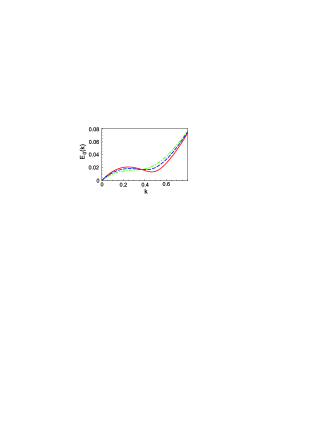
Figure 1: Collective mode spectrum calculated for $d=5a_{0}$ and $n=4\cdot 10^{-3}a_{0}^{-2}$ (solid curve), $n=3\cdot 10^{-3}a_{0}^{-2}$ (dashed curve), and $n=2\cdot 10^{-3}a_{0}^{-2}$ (dash-dotted curve). The energy $E_{0}(k)$ is given in units of $e^{2}/\varepsilon a_{0}=2Ry_{eff}$ (doubled effective Rydberg), and $k$ in units of $a_{0}^{-1}$.

III Kinematic approach

To obtain the wave crest pattern generated by a point obstacle, we use the kinematic approach [1]. We consider the two-dimensional problem in the rest frame with the obstacle at the origin and the flow velocity vector $\mathbf{V}=(-V,0)$. In this frame of reference the stationary wave crests do not move. The condition of that is

$$\hbar\omega(k)=E_{0}(k)-\hbar kV\cos\xi=0,$$ (30)

where $\xi$ is the angle between the wave vector $\mathbf{k}$ and the $x$ axis. Equation (30) implicitly defines the functions $k(\xi)$ and $k_{x}(k_{y})$ ($k_{x}$, $k_{y}$ are the components of $\mathbf{k}$ and $k$ is its modulus). In the general case, these functions are multiple valued. The number of branches is equal to the number of intersections of the dispersion curve, $\omega=E_{0}(k)$, with the line $\omega=Vk\cos\xi$.

The phase of the stationary wave is given by the integral

$$\theta(\bf{r})=\int_{0}^{\bf{r}}\mathbf{k}(\mathbf{r}^{\prime})d\mathbf{r}^{\prime}.$$ (31)

It follows from (31) that the components of $\mathbf{k}$ satisfy the relation

$$\frac{\partial k_{y}}{\partial x}=\frac{\partial k_{x}}{\partial y}.$$ (32)

The right-hand side of Eq. (32) can be expressed through the derivative of the function $k_{x}(k_{y})$: ${\partial k_{x}}/{\partial y}=({dk_{x}}/{dk_{y}})({\partial k_{y}}/{\partial y})$. Substituting the function $k_{x}(k_{y})$ into (30) we obtain the identity

$$E_{0}\left(\sqrt{[k_{x}(k_{y})]^{2}+k_{y}^{2}}\right)-\hbar Vk_{x}(k_{y})\equiv 0.$$ (33)

The derivative of the left-hand side of Eq. (33) with respect to $k_{y}$ is equal to zero. It yields

$$\frac{dk_{x}}{dk_{y}}=-\frac{\frac{dE_{0}}{dk}\frac{k_{y}}{k}}{\frac{dE_{0}}{dk}\frac{k_{x}}{k}-\hbar V}.$$ (34)

Equation (34) can be rewritten as

$$\frac{dk_{x}}{dk_{y}}=-\frac{{v}_{g,y}}{{v}_{g,x}},$$ (35)

where ${v}_{g,x}$ and ${v}_{g,y}$ are the components of

$$\mathbf{v}_{g}(\mathbf{k})=\frac{d\omega(\mathbf{k})}{d\mathbf{k}},$$ (36)

the group velocity of collective excitations in the rest frame.

It follows from Eqs. (32) and (35) that the components of the vector $\mathbf{k}$ are the constants along the line

$$\frac{x}{y}=\frac{{v}_{g,x}}{{v}_{g,y}}.$$ (37)

This line is along the group velocity (36). Thus the group velocity $\mathbf{v}_{g}(\mathbf{k})$ determines the direction of propagation of the stationary wave, with the wave vector $\mathbf{k}$, in the rest frame of reference. The integral (31) calculated along the line $\mathbf{k}=const$ is equal to

$$\theta(r,\xi)=kr\cos(\xi-\chi),$$ (38)

where $\chi$ is the angle between the group velocity (36) and the $x$ axis. The angle $\chi$ is the function of $\xi$. The dependence $\chi(\xi)$ can be found from the expressions for the components of $\mathbf{v}_{g}$ at $k=k(\xi)$:

$${v}_{g,x}(\xi)=\frac{1}{\hbar}\frac{dE_{0}(k)}{dk}\Big{|}_{k=k(\xi)}\cos\xi-V,\quad{v}_{g,y}(\xi)=\frac{1}{\hbar}\frac{dE_{0}(k)}{dk}\Big{|}_{k=k(\xi)}\sin\xi.$$ (39)

At the crest lines, the phase (38) is a multiply of $2\pi$,

$$\theta_{N}(\xi)=2\pi N\mathrm{sign}[\cos[\xi-\chi(\xi)]],$$ (40)

where $N=1,2,3,\ldots$. The function $\mathrm{sign}(x)$ in (40) takes into account that the sign of $\theta$ in Eq.(38) coincides with the sign of $\cos(\xi-\xi)$ ( by definition, $k$ and $r$ are the positive quantities).

From Eq. (38), we obtain the parametric equations that determine the crest lines

$$x_{N}(\xi) = \frac{\theta_{N}(\xi)\cos[\chi(\xi)]}{k(\xi)\cos[\xi-\chi(\xi)]},$$ (41)

$$y_{N}(\xi) = \frac{\theta_{N}(\xi)\sin[\chi(\xi)]}{k(\xi)\cos[\xi-\chi(\xi)]}.$$ (42)

Taking into account the relations (30) and (39) we present Eqs. (41) in the form

$$x_{N}(\xi) = 2\pi N\frac{v_{g0}(\xi)\cos\xi-V}{k(\xi)\left[v_{g0}(\xi)-v_{p0}(\xi)\right]}\mathrm{sign}\left[v_{g0}(\xi)-v_{p0}(\xi)\right],$$ (43)

$$y_{N}(\xi) = 2\pi N\frac{v_{g0}(\xi)\sin\xi}{k(\xi)\left[v_{g0}(\xi)-v_{p0}(\xi)\right]}\mathrm{sign}\left[v_{g0}(\xi)-v_{p0}(\xi)\right],$$ (44)

where $v_{g0}(\xi)=(dE_{0}(k)/dk)|_{k=k(\xi)}$ and $v_{p0}(\xi)=E_{0}(k)/k|_{k=k(\xi)}$, respectively, are the group and the phase velocities of the collective mode in the condensate at rest (negative $v_{g0}$ corresponds to oppositely directed $\mathbf{v}_{g0}$ and $\mathbf{k}$). The functions $v_{g0}(\xi)$, $v_{p0}(\xi)$, $x_{N}(\xi)$ and $y_{N}(\xi)$ have the same number of branches as the function $k(\xi)$ has. For the dispersion curves shown in Fig. 1 the function $k(\xi)$ has two branches, the lower and the upper ones. The lower branch corresponds to $k$ for which $v_{g0}<v_{p0}$, and the upper branch corresponds to $k$ for which $v_{g0}>v_{p0}$.

One can see from (43) that the intersections of the crest lines with the $x$ axis correspond to $\xi=0$ or to $v_{g0}(\xi)=0$. For the upper branch of $k(\xi)$, the velocity $v_{g0}\neq 0$ for all $\xi$ and the $N$-th crest line intersects the $x$ axis only once [at $x=x_{N}(0)$]. There can be up to three intersections for the crest line associated with the lower branch of $k(\xi)$. The number of intersections depends on the presence (absence) of the roton-type minimum and on the value of $V$. At $v_{g0}(\xi)=v_{p0}(\xi)$ the coordinates $x_{N}(\xi)$ and $y_{N}(\xi)$ approach infinity. The condition $v_{g0}=v_{p0}$ is reached at $k\to 0$ and at the minimum of the phase velocity.

To illustrate the complexity of the wave crest pattern we consider the system far from the superfluid-supersolid transition line and the system close to the transition line. The spectrum of the system far from the transition line (dash-dotted curve in Fig. 1) has no roton-type minimum. One can distinguish two special phase velocities: $v_{0}$, the sound velocity at $k\to 0$, and $v_{min}$, the minimum phase velocity. The convenient units for the velocities are $2Ry_{eff}a_{0}/\hbar=\alpha c/\varepsilon$, where $c$ is the speed of light, and $\alpha\approx 1/137$ is the fine structure constant. In these units $v_{0}\approx 0.128$ and $v_{min}\approx 0.045$ at $n=2\cdot 10^{-3}a_{0}^{-2}$ and $d=5a_{0}$. In Fig. 2, the wave crest patterns calculated for $V=0.16$, $V=0.1$, and $V=0.06$ are presented. One can see that the stationary wave patterns at $V>v_{0}$ and $v_{0}>V>v_{min}$ differ from each other. In the former case stationary waves are not excited in a narrow wedge behind the obstacle. In the latter case stationary waves fill all the space. At $V<v_{min}$, stationary waves are not excited. Within the range $v_{0}>V>v_{min}$, the pattern is changed qualitatively under variation in the flow velocity: at larger $V$, the wave crests have cusps and self-intersections, and at smaller $V$, the cusps and intersections disappear.

One can distinguish four special velocities for the system close to the superfluid-supersolid transition line. Two of them, $v_{0}$ and $v_{min}$, are defined above. Two other velocities, $v_{1}$ and $v_{2}$, are the phase velocities at the local maximum and at the local minimum in the dispersion curve $E_{0}(k)$. For $n=4\cdot 10^{-3}a_{0}^{-2}$ and $d=5a_{0}$, the special velocities are $v_{0}\approx 0.18$, $v_{1}=0.085$, $v_{2}=0.0287$ and $v_{min}=0.0281$ (in $\alpha c/\varepsilon$ units). In Fig. 3, we present the crest line patterns for $V=0.19$ ($V>v_{0}$), $V=0.16$ ($v_{0}>V>v_{1}$), $V=0.06$ ($v_{1}>V>v_{2}$), and $V=0.0285$ ($v_{2}>V>v_{min}$). One can see that in this case, the wave crest pattern is also modified significantly under variation in the flow velocity.

In all cases, the wave crest pattern contains a family of crests located outside the wedge-shaped region with the semiangle $\theta=\arccos(v_{min}/V)$. A similar family is observed in Bose gases with contact interaction [2, 3, 4, 5, 6]. The other families of crests (absent in the atomic BEC) are located entirely behind the obstacle. In the general case, they contain cusps and intersections.

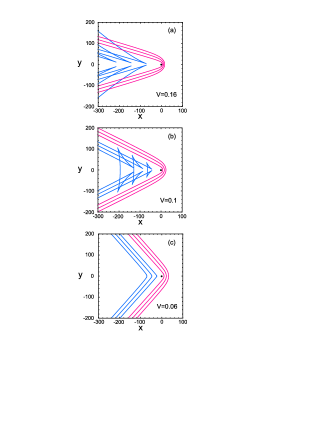
Figure 2: Crests of stationary waves induced by a point obstacle at $n=2\cdot 10^{-3}a_{0}^{-2}$ and $d=5a_{0}$. The flow velocity is equal to (a) $V=0.16$, (b) $V=0.1$, and (c) $V=0.06$ in $\alpha c/\varepsilon$ units. Red (blue) crests correspond to the collective modes with $v_{g0}<v_{p0}$ ($v_{g0}>v_{p0}$). Only the first three crests are shown. The black dot indicates the obstacle location. The spatial scale unit is $a_{0}$.

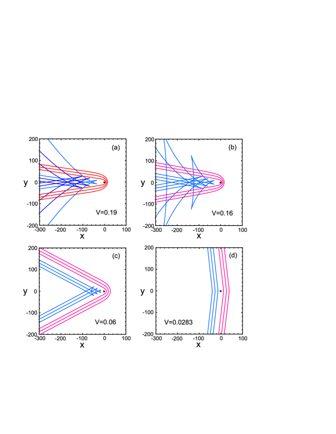
Figure 3: The same as in Fig. 2 for $n=4\cdot 10^{-3}a_{0}^{-2}$, $d=5a_{0}$, and the flow velocity (a) $V=0.19$, (b) $V=0.16$, (c) $V=0.06$, and (d) $V=0.0283$ (in $\alpha c/\varepsilon$ units).

IV Dynamical approach

For the comparison of the theory with the experiment, it is instructive to find relative amplitudes of stationary waves. It can be done in the framework of the dynamical approach [1].

To apply the dynamical approach to the BEC of spatially indirect excitons, we take into account the interaction with the obstacle in Eq. (8),

$$i\hbar\frac{\partial}{\partial t}\Psi({\bf R}_{12},t)=-\frac{\hbar^{2}}{2M}\frac{\partial^{2}}{\partial\mathbf{R}_{12}^{2}}\Psi({\bf R}_{12},t)+U(\mathbf{R}_{12})\Psi({\bf R}_{12},t)$$ (45)

$$+\int d{\bf r}_{12}d{\bf r}_{3}d{\bf r}_{4}\left[A[{\bf r}_{i}]\Psi({\bf R}_{12},t)|\Psi({\bf R}_{34},t)|^{2}+B[{\bf r}_{i}]\Psi({\bf R}_{32},t)\Psi^{*}({\bf R}_{34},t)\Psi({\bf R}_{14},t)\right].$$ (46)

The potential $U(\mathbf{R})$ describes the interaction of an electron-hole pair, which center of mass has the coordinate $\mathbf{R}$, with the obstacle at the origin. The solution of (45) is sought in the form

$$\Psi({\bf R},t)=\Psi_{0}({\bf R},t)+\Psi_{1}({\bf R},t)=e^{-i\frac{\mu}{\hbar}t}e^{i\mathbf{R}\nabla\varphi}\left[\sqrt{n}+\tilde{\Psi}_{1}({\bf R},t)\right].$$ (47)

The first term in the square brackets in (47) corresponds to the uniform condensate. The term $\Psi_{1}({\bf R},t)$ is caused by the interaction with the obstacle. The point obstacle is modeled by the potential

$$U(\mathbf{R},t)=U_{0}\delta(\mathbf{R})e^{\eta t},$$ (48)

where $\eta=+0$. We imply that the interaction with the obstacle was switched on at $t\to-\infty$ and look for a response at $t=0$. The response is assumed to be small, linear in $U_{0}$. The divergence of (48) at $t\to\infty$ is not relevant because due to the casuality principle the response of the system to the obstacle at $t=t_{0}$ depends on $U(\mathbf{R},t^{\prime})$ with $t^{\prime}\leq t_{0}$. The time dependence of $\tilde{\Psi}_{1}({\bf R},t)$ has the form $\tilde{\Psi}_{1}({\bf R},t)=\tilde{\Psi}_{1}({\bf R})e^{\eta t}$. In the linear in $U_{0}$ order we obtain the following equation for $\tilde{\Psi}_{1}(\mathbf{R})$:

$$-\frac{\hbar^{2}}{2M}\frac{\partial^{2}}{\partial\mathbf{R}_{12}^{2}}\tilde{\Psi}_{1}({\bf R}_{12})-i\hbar\mathbf{V}\cdot\frac{\partial}{\partial\mathbf{R}_{12}}\tilde{\Psi}_{1}({\bf R}_{12})-i\hbar\eta\tilde{\Psi}_{1}({\bf R}_{12})$$ (49)

$$+\int d{\bf r}_{12}d{\bf r}_{3}d{\bf r}_{4}A[{\bf r}_{i}]{n}\left[\tilde{\Psi}_{1}({\bf R}_{34})+\tilde{\Psi}^{*}_{1}({\bf R}_{34})\right]$$ (50)

$$+\int d{\bf r}_{12}d{\bf r}_{3}d{\bf r}_{4}B[{\bf r}_{i}]{n}\left[\tilde{\Psi}_{1}({\bf R}_{32})+\tilde{\Psi}_{1}({\bf R}_{14})+\tilde{\Psi}^{*}_{1}({\bf R}_{34})-\tilde{\Psi}_{1}({\bf R}_{12})\right]=-\sqrt{n}U_{0}\delta(\mathbf{R}_{12}).$$ (51)

From (49), we find the system of equations for the Fourier components of $\tilde{\Psi}_{1}(\mathbf{R})$:

$$\left[\epsilon_{k}+\hbar(\mathbf{k}\mathbf{V}-i\eta)+(\gamma_{k}^{(d)}+\gamma_{k}^{(ex,1)})n\right]\tilde{\Psi}_{1}({\bf k})+(\gamma_{k}^{(d)}+\gamma_{k}^{(ex,2)})n\tilde{\Psi}^{*}_{1}({-\bf k})=-\sqrt{n}U_{0},$$ (52)

$$(\gamma_{k}^{(d)}+\gamma_{k}^{(ex,2)})n\tilde{\Psi}_{1}({\bf k})+\left[\epsilon_{k}-\hbar(\mathbf{k}\mathbf{V}-i\eta)+(\gamma_{k}^{(d)}+\gamma_{k}^{(ex,1)})n\right]\tilde{\Psi}^{*}_{1}(-{\bf k})=-\sqrt{n}U_{0}.$$ (53)

In obtaining (52) we take into account that $\gamma_{k}^{(d)}$ and $\gamma_{k}^{(ex,i)}$ depend on the modulus $\mathbf{k}$. The solution of the system (52) is

$$\tilde{\Psi}_{1}({\bf k})=-\frac{\epsilon_{k}+(\gamma_{k}^{(ex,1)}-\gamma_{k}^{(ex,2)})n-\hbar(\mathbf{k}\mathbf{V}-i\eta)}{[E_{0}(k)]^{2}-\hbar^{2}(\mathbf{k}\mathbf{V}-i\eta)^{2}}\sqrt{n}U_{0}.$$ (54)

In the same order in $U_{0}$ the spatial variation of the density is given by the equation

$$\delta n(\mathbf{r})=\sqrt{n}\left[\tilde{\Psi}_{1}({\bf r})+\tilde{\Psi}_{1}^{*}({\bf r})\right]=\frac{\sqrt{n}}{(2\pi)^{2}}\int d^{2}ke^{i\mathbf{k}\mathbf{r}}\left[\tilde{\Psi}_{1}({\bf k})+\tilde{\Psi}_{1}^{*}(-{\bf k})\right].$$ (55)

Substitution of (54) into (55) yields

$$\delta n(\mathbf{r})=-\frac{nU_{0}}{2\pi^{2}}\int d\mathbf{k}e^{i\mathbf{k}\mathbf{r}}\frac{\epsilon_{k}+(\gamma_{k}^{(ex,1)}-\gamma_{k}^{(ex,2)})n}{[E_{0}(k)]^{2}-\hbar^{2}(\mathbf{k}\mathbf{V}-i\eta)^{2}}.$$ (56)

Introducing the polar angle $\chi$ [$\mathbf{r}=(r\cos\chi,r\sin\chi)$] and considering $\mathbf{V}=(-V,0)$, we get

$$\delta n(\mathbf{r})=-\frac{nU_{0}}{\pi^{2}}\mathrm{Re}\int_{-\frac{\pi}{2}}^{\frac{\pi}{2}}d\xi\int_{0}^{\infty}dke^{ikr\cos(\xi-\chi)}\frac{k\left[\epsilon_{k}+(\gamma_{k}^{(ex,1)}-\gamma_{k}^{(ex,2)})n\right]}{[E_{0}(k)]^{2}-\hbar^{2}(kV\cos\xi+i\eta)^{2}}.$$ (57)

In obtaining (57), we take into account that the integrand in Eq.(57) transforms into the complex conjugated expression under substitution, $\xi\to\xi+\pi$.

We evaluate the integral over $k$ in Eq. (57) using the residue theorem. Then we calculate the integral over $\xi$ in the stationary phase approximation. Details are given in Appendix B. The answer has the form

$$\delta n(\mathbf{r})={nU_{0}}\sqrt{\frac{2}{\pi}}\sum_{\lambda,i}\left[\frac{\sin\left[f_{\lambda}(\xi)+\frac{\pi}{4}\mathrm{sign}[f^{\prime\prime}_{\lambda}(\xi)]\right]}{\sqrt{|f^{\prime\prime}_{\lambda}(\xi)|}}s_{\lambda}[\xi,\chi]\right]\left[\frac{k\left[\epsilon_{k}+(\gamma_{k}^{(ex,1)}-\gamma_{k}^{(ex,2)})n\right]}{E_{0}(k)\left[\frac{dE_{0}(k)}{dk}-\frac{E_{0}(k)}{k}\right]}\right]\Bigg{|}_{\begin{array}[]{c}k=k_{\lambda}(\xi),\\ \xi=\xi_{\lambda,i}(\chi)\end{array}},$$ (58)

where the index $\lambda$ is the branch number of the multivalued function $k(\xi)$ defined in the previous section,

$$f_{\lambda}(\xi)=k_{\lambda}(\xi)r\cos(\chi-\xi)$$ (59)

is the phase of the exponent in (57), and $\xi_{\lambda}(\chi)$ is the function reciprocal to the function $\chi_{\lambda}(\xi)$ introduced in the previous section. In the general case, the function $\xi_{\lambda}(\chi)$ at given $\lambda$ is multivalued and the index $i$ is the branch number of this function at fixed $\lambda$. The factor $s_{\lambda}[\xi,\chi]$ in Eq. (58) is defined as

$$s_{\lambda}(\xi,\chi)=\left\{\begin{array}[]{ll}1,&\hbox{ if $\left(\frac{dE_{0}(k)}{dk}-\frac{E_{0}(k)}{k}\right)\Big{|}_{k=k_{\lambda}(\xi)}<0$ and $\cos(\xi-\chi)<0$;}\\ -1,&\hbox{ if $\left(\frac{dE_{0}(k)}{dk}-\frac{E_{0}(k)}{k}\right)\Big{|}_{k=k_{\lambda}(\xi)}>0$ and $\cos(\xi-\chi)>0$;}\\ 0,&\hbox{otherwise.}\end{array}\right.$$ (60)

The amplitude of spatial oscillations of $\delta n(\mathbf{r})$ (58) is proportional to $1/\sqrt{r}$, where $r$ is the distance from the obstacle. The contribution proportional to $1/r^{2}$ is neglected in (58) (see Appendix B).

In Fig. 4, we present the density plot of $\delta n(\mathbf{r})$ (the stationary wave pattern) calculated for the same parameters as in Fig. 2. One can see that some wave crests shown in Figs. 2(a) and 2(b), are invisible in the density plots Figs. 4(a) and 4(b). These wave crests correspond to modes with small $k$. Indeed, summands in Eq. (58) are proportional to $k^{3/2}$ at small $k$ and, due to this, the relative amplitudes of stationary waves that correspond to long-wave modes are small.

In Fig. 5, we present the stationary wave pattern calculated for the same parameters as in Fig. 3. Again we see that stationary waves with small $k$ are practically invisible in the density plots.

The changes in the stationary wave pattern under variation in the flow velocity are less spectacular than the changes in the wave crest pattern. Nevertheless, the stationary wave pattern differs significantly from the one obtained for the atomic BEC [4, 5, 6] and it is modified qualitatively with a change in the flow velocity and in the density of the condensate.

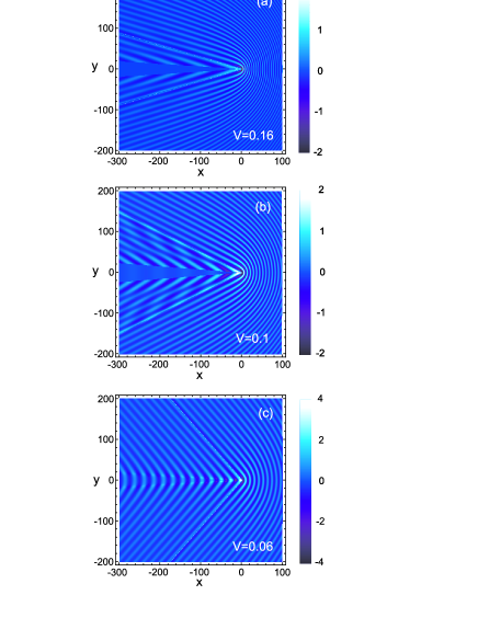
Figure 4: Stationary wave pattern induced by the point obstacle in the system far from the superfluid-supersolid transition line ($n=2\cdot 10^{-3}a_{0}^{-2}$ and $d=5a_{0}$). The flow velocities $V$ are given in $c/137\varepsilon$ units. The density variation $\delta n$ is given in units of $nU_{0}/(2Ry_{eff}a_{0})$.

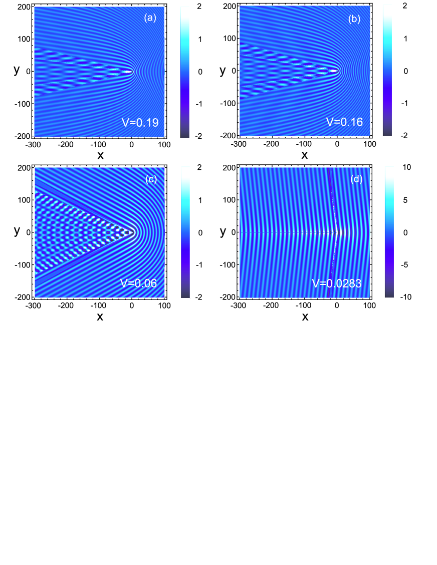
Figure 5: Stationary wave pattern induced by the point obstacle in the system close to the superfluid-supersolid transition line ($n=4\cdot 10^{-3}a_{0}^{-2}$ and $d=5a_{0}$). The flow velocities $V$ are given in $c/137\varepsilon$ units. The density variation $\delta n$ is given in units of $nU_{0}/(2Ry_{eff}a_{0})$.

To visualize stationary waves caused by the long-wave part of the spectrum, one can use a weak extended obstacle instead of the point one. To illustrate this possibility, we consider the obstacle in which the interaction with electron-hole pairs is described by the Gaussian potential

$$U(\mathbf{R})=\frac{U_{0}}{2\pi a^{2}}\exp\left(-\frac{R^{2}}{2a^{2}}\right).$$ (61)

The potential (61) is normalized by the same condition as the potential (48):

$$\int d^{2}rU(\mathbf{r})=U_{0}.$$ (62)

The Fourier components of the potential (61) are equal to

$$U(\mathbf{k})=U(k)=U_{0}\exp\left(-\frac{k^{2}a^{2}}{2}\right).$$ (63)

For the potential (61), the dynamical approach yields

$$\delta n(\mathbf{r})={n}\sqrt{\frac{2}{\pi}}\sum_{\lambda,i}U(k)\frac{\sin\left[f_{\lambda}(\xi)+\frac{\pi}{4}\mathrm{sign}[f^{\prime\prime}_{\lambda}(\xi)]\right]}{\sqrt{|f^{\prime\prime}_{\lambda}(\xi)|}}s_{\lambda}[\xi,\chi]\left[\frac{k\left[\epsilon_{k}+(\gamma_{k}^{(ex,1)}-\gamma_{k}^{(ex,2)})n\right]}{E_{0}(k)\left[\frac{E_{0}(k)}{dk}-\frac{E_{0}(k)}{k}\right]}\right]\Bigg{|}_{\begin{array}[]{c}k=k_{\lambda}(\xi),\\ \xi=\xi_{\lambda,i}(\chi)\end{array}}$$ (64)

Equation (64) differs from Eq. (58) by the factor $U(k)$.

We specify the case $a\gg a_{0}$. In this case, the factor $U(k)$ suppresses the short-wave contribution into $\delta n(\mathbf{r})$ and the long-wave contribution becomes visible. The stationary wave patterns calculated for the potential (61) with $a=10a_{0}$ are shown in Figs. 6 and 7. One can see that the wave crests hidden in Figs. 4 and 5 are easily identified in Figs. 6 and 7, and vice versa. The patterns in Figs. 6(b) and 7(b) resemble ship waves on a surface of deep water. The waves in Figs. 6(b) and 7(b) fill the wedge-shaped region behind the obstacle, but the semiangle of this wedge is not a universal quantity. As in the previous case, the stationary wave pattern is modified qualitatively under variation in the exciton density and under variation in the flow velocity.

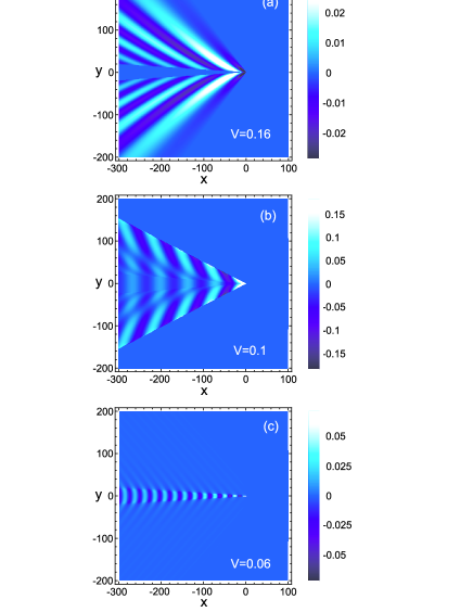
Figure 6: The stationary wave patterns induced by a weak extended obstacle for $n=2\cdot 10^{-3}a_{0}^{-2}$ and $d=5a_{0}$. The flow velocities are the same as in Fig. 4. The interaction of the obstacle with electron-hole pairs is described by the Gaussian potential (61) with $a=10a_{0}$.

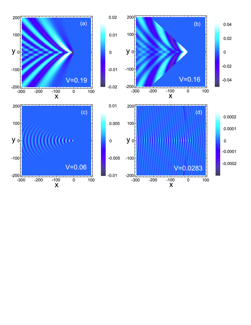
Figure 7: The stationary wave patterns induced by a weak extended obstacle for $n=4\cdot 10^{-3}a_{0}^{-2}$ and $d=5a_{0}$. The flow velocities are the same as in Fig. 5. The interaction of the obstacle with electron-hole pairs is described by the Gaussian potential (61) with $a=10a_{0}$.

The spatial resolution should not be less than $(20-40)a_{0}$ to observe the stationary wave patterns shown in Figs. 6(a), 6(b) and in Figs. 7(a), 7(b). In the case of GaAs heterostructures, it corresponds to 200-400 nm. That is the maximum resolution achieved in photoluminescence experiments with spatially indirect excitons [66]. At lower resolutions, one can also observe stationary waves, but only at a large distance from the obstacle. In TMD double layer systems, the effective Bohr radius is ten times smaller then in GaAs and the resolution that can be achieved in photoluminescence experiments is too low to observe the stationary wave pattern in such structures. Much better spatial resolution (about 10 nm) was achieved in [67] by the method of probing of excitons in [67] based on obtaining the low-energy loss spectra using the scanning transmission electron microscope. We may also suggest to register stationary waves by measuring the spatial variation of the electrostatic potential near the bilayer system. The most effective method of measuring the local electrostatic potential uses the single-electron transistor (SET) technique [68]. This method provides spatial resolution of the order of the SET size that can be about 100 nm. We also suggest to use the stationary wave pattern [especially the pattern shown Fig. 6(d)] as a grating for a generation of short-wave plasmons in a nearby conducting layer.

V Conclusion

In conclusion we have considered stationary waves occurring in the BEC of spatially indirect excitons in bilayers. Under an increase in the exciton density or in the distance between the layers the uniform state of the exciton condensate becomes unstable with respect to the transition to the supersolid state. The roton-type minimum in the collective mode spectrum emerges as a precursor of such a transition. The presence of this minimum reveals itself in a number of features in the stationary wave pattern. The observation of such features and qualitative changes in the stationary wave pattern under an increase in the exciton density can be a bright manifestation of superfluidity of the exciton gas and its proximity to the superfluid-supersolid transition line.

Two possible systems where the effects predicted in this paper can be observed are TMD bilayers and double quantum well GaAs heterostructures. The advantage of the former ones is much larger critical temperatures while for the latter the lower spatial resolution is required to observe stationary waves.

Appendix A Collective mode spectrum in a system with different electron and hole effective masses in the three-layer dielectric matrix

Equations (25)-(27) can be easily generalized for $m_{e}\neq m_{h}$ and different $V_{ee}(r)$ and $V_{hh}(r)$.

The functions (19)-(21) written through the Fourier components have the form

$$\gamma^{(d)}_{\bf k}=V_{ee}(\mathbf{k})\int\frac{d^{2}p}{(2\pi)^{2}}\frac{d^{2}p^{\prime}}{(2\pi)^{2}}\phi^{*}_{\mathbf{p}+\tilde{m}_{h}\mathbf{k}}\phi_{\mathbf{p}}\phi^{*}_{\mathbf{p}^{\prime}-\tilde{m}_{h}\mathbf{k}}\phi_{\mathbf{p}^{\prime}}+V_{hh}(\mathbf{k})\int\frac{d^{2}p}{(2\pi)^{2}}\frac{d^{2}p^{\prime}}{(2\pi)^{2}}\phi^{*}_{\mathbf{p}-\tilde{m}_{e}\mathbf{k}}\phi_{\mathbf{p}}\phi^{*}_{\mathbf{p}^{\prime}+\tilde{m}_{e}\mathbf{k}}\phi_{\mathbf{p}^{\prime}}$$ (65)

$$+V_{eh}(\mathbf{k})\int\frac{d^{2}p}{(2\pi)^{2}}\frac{d^{2}p^{\prime}}{(2\pi)^{2}}\Big{[}\phi^{*}_{\mathbf{p}+\tilde{m}_{h}\mathbf{k}}\phi_{\mathbf{p}}\phi^{*}_{\mathbf{p}^{\prime}+\tilde{m}_{e}\mathbf{k}}\phi_{\mathbf{p}^{\prime}}+\phi^{*}_{\mathbf{p}-\tilde{m}_{e}\mathbf{k}}\phi_{\mathbf{p}}\phi^{*}_{\mathbf{p}^{\prime}-\tilde{m}_{h}\mathbf{k}}\phi_{\mathbf{p}^{\prime}}\Big{]},$$ (66)

$$\gamma^{(ex,1)}_{\bf k}=-\int\frac{d^{2}p}{(2\pi)^{2}}\frac{d^{2}q}{(2\pi)^{2}}\Big{[}V_{ee}(\mathbf{p})\Big{(}\phi^{*}_{\mathbf{q}}\phi_{\mathbf{q}}\phi^{*}_{\mathbf{q}-\mathbf{p}+\tilde{m}_{e}\mathbf{k}}\phi_{\mathbf{q}-\mathbf{p}+\tilde{m}_{e}\mathbf{k}}+\phi^{*}_{\mathbf{q}}\phi_{\mathbf{q}-\tilde{m}_{h}\mathbf{k}}\phi^{*}_{\mathbf{q}-\mathbf{p}-\tilde{m}_{h}\mathbf{k}}\phi_{\mathbf{q}-\mathbf{p}}-\phi^{*}_{\mathbf{q}}\phi_{\mathbf{q}}\phi^{*}_{\mathbf{q}-\mathbf{p}}\phi_{\mathbf{q}-\mathbf{p}}\Big{)}$$ (67)

$$+V_{hh}(\mathbf{p})\Big{(}\phi^{*}_{\mathbf{q}}\phi_{\mathbf{q}+\mathbf{p}}\phi^{*}_{\mathbf{q}+\mathbf{p}+\tilde{m}_{e}\mathbf{k}}\phi_{\mathbf{q}+\tilde{m}_{e}\mathbf{k}}+\phi^{*}_{\mathbf{q}}\phi_{\mathbf{q}+\mathbf{p}-\tilde{m}_{h}\mathbf{k}}\phi^{*}_{\mathbf{q}+\mathbf{p}-\tilde{m}_{h}\mathbf{k}}\phi_{\mathbf{q}}-\phi^{*}_{\mathbf{q}}\phi_{\mathbf{q}+\mathbf{p}}\phi^{*}_{\mathbf{q}+\mathbf{p}}\phi_{\mathbf{q}}\Big{)}\Big{]}$$ (68)

$$+\frac{1}{2}\int\frac{d^{2}p}{(2\pi)^{2}}\frac{d^{2}q}{(2\pi)^{2}}V_{eh}(\mathbf{p})\Big{[}\phi^{*}_{\mathbf{q}+\mathbf{p}}\phi_{\mathbf{q}}\phi^{*}_{\mathbf{q}+\tilde{m}_{e}\mathbf{k}}\phi_{\mathbf{q}+\tilde{m}_{e}\mathbf{k}}+\phi^{*}_{\mathbf{q}}\phi_{\mathbf{q}}\phi^{*}_{\mathbf{q}+\mathbf{p}+\tilde{m}_{e}\mathbf{k}}\phi_{\mathbf{q}+\tilde{m}_{e}\mathbf{k}}+\phi^{*}_{\mathbf{q}}\phi_{\mathbf{q}}\phi^{*}_{\mathbf{q}+\tilde{m}_{e}\mathbf{k}}\phi_{\mathbf{q}+\mathbf{p}+\tilde{m}_{e}\mathbf{k}}$$ (69)

$$+\phi^{*}_{\mathbf{q}}\phi_{\mathbf{q}+\mathbf{p}}\phi^{*}_{\mathbf{q}+\tilde{m}_{e}\mathbf{k}}\phi_{\mathbf{q}+\tilde{m}_{e}\mathbf{k}}+\phi^{*}_{\mathbf{q}+\mathbf{p}}\phi_{\mathbf{q}-\tilde{m}_{h}\mathbf{k}}\phi^{*}_{\mathbf{q}-\tilde{m}_{h}\mathbf{k}}\phi_{\mathbf{q}}+\phi^{*}_{\mathbf{q}}\phi_{\mathbf{q}-\tilde{m}_{h}\mathbf{k}}\phi^{*}_{\mathbf{q}+\mathbf{p}-\tilde{m}_{h}\mathbf{k}}\phi_{\mathbf{q}}+\phi^{*}_{\mathbf{q}}\phi_{\mathbf{q}-\tilde{m}_{h}\mathbf{k}}\phi^{*}_{\mathbf{q}-\tilde{m}_{h}\mathbf{k}}\phi_{\mathbf{q}+\mathbf{p}}$$ (70)

$$+\phi^{*}_{\mathbf{q}}\phi_{\mathbf{q}+\mathbf{p}-\tilde{m}_{h}\mathbf{k}}\phi^{*}_{\mathbf{q}-\tilde{m}_{h}\mathbf{k}}\phi_{\mathbf{q}}-2\phi^{*}_{\mathbf{q}+\mathbf{p}}\phi_{\mathbf{q}}\phi^{*}_{\mathbf{q}}\phi_{\mathbf{q}}-2\phi^{*}_{\mathbf{q}}\phi_{\mathbf{q}+\mathbf{p}}\phi^{*}_{\mathbf{q}}\phi_{\mathbf{q}}\Big{]},$$ (71)

$$\gamma^{(ex,2)}_{\bf k}=-\int\frac{d^{2}p}{(2\pi)^{2}}\frac{d^{2}q}{(2\pi)^{2}}\Big{[}V_{ee}(\mathbf{p})\phi^{*}_{\mathbf{q}-\tilde{m}_{e}\mathbf{k}}\phi_{\mathbf{q}-\mathbf{k}}\phi^{*}_{\mathbf{q}-\mathbf{p}-\tilde{m}_{h}\mathbf{k}}\phi_{\mathbf{q}-\mathbf{p}}+V_{hh}(\mathbf{p})\phi^{*}_{\mathbf{q}-\tilde{m}_{e}\mathbf{k}}\phi_{\mathbf{q}+\mathbf{p}-\mathbf{k}}\phi^{*}_{\mathbf{q}+\mathbf{p}-\tilde{m}_{h}\mathbf{k}}\phi_{\mathbf{q}}\Big{]}$$ (72)

$$+\frac{1}{2}\int\frac{d^{2}p}{(2\pi)^{2}}\frac{d^{2}q}{(2\pi)^{2}}V_{eh}(\mathbf{p})\Big{[}\phi^{*}_{\mathbf{q}+\mathbf{p}-\tilde{m}_{e}\mathbf{k}}\phi_{\mathbf{q}-\mathbf{k}}\phi^{*}_{\mathbf{q}-\tilde{m}_{h}\mathbf{k}}\phi_{\mathbf{q}}+\phi^{*}_{\mathbf{q}-\tilde{m}_{e}\mathbf{k}}\phi_{\mathbf{q}-\mathbf{k}}\phi^{*}_{\mathbf{q}+\mathbf{p}-\tilde{m}_{h}\mathbf{k}}\phi_{\mathbf{q}}$$ (73)

$$+\phi^{*}_{\mathbf{q}-\tilde{m}_{e}\mathbf{k}}\phi_{\mathbf{q}-\mathbf{k}}\phi^{*}_{\mathbf{q}-\tilde{m}_{h}\mathbf{k}}\phi_{\mathbf{q}+\mathbf{p}}+\phi^{*}_{\mathbf{q}-\tilde{m}_{e}\mathbf{k}}\phi_{\mathbf{q}+\mathbf{p}-\mathbf{k}}\phi^{*}_{\mathbf{q}-\tilde{m}_{h}\mathbf{k}}\phi_{\mathbf{q}}\Big{]},$$ (74)

where $\phi_{\mathbf{q}}$, $V_{ee}(\mathbf{k})$, $V_{hh}(\mathbf{k})$, and $V_{eh}(\mathbf{k})$ are the Fourier components of the function $\phi_{0}(\mathbf{r})$, and of the potentials $V_{ee}(\mathbf{r})$, $V_{hh}(\mathbf{r})$, and $V_{eh}(\mathbf{r})$, respectively, and we use the notation $\tilde{m}_{e(h)}={m}_{e(h)}/({m}_{e}+m_{h})$.

For the three-layer dielectric matrix the Fourier components of the Coulomb potentials can be approximated as

$$V_{ee}({\mathbf{k}}) = \frac{4\pi e^{2}}{k}\frac{\varepsilon_{2}+\varepsilon_{3}+(\varepsilon_{2}-\varepsilon_{3})e^{-2kd}}{(\varepsilon_{2}+\varepsilon_{3})(\varepsilon_{2}+\varepsilon_{1})-{(\varepsilon_{2}-\varepsilon_{3})(\varepsilon_{2}-\varepsilon_{1})}e^{-2kd}},$$ (75)

$$V_{hh}({\mathbf{k}}) = \frac{4\pi e^{2}}{k}\frac{\varepsilon_{2}+\varepsilon_{1}+(\varepsilon_{2}-\varepsilon_{1})e^{-2kd}}{(\varepsilon_{2}+\varepsilon_{3})(\varepsilon_{2}+\varepsilon_{1})-{(\varepsilon_{2}-\varepsilon_{3})(\varepsilon_{2}-\varepsilon_{1})}e^{-2kd}},$$ (76)

$$V_{eh}({\mathbf{k}}) = -\frac{8\pi e^{2}}{k}\frac{{\varepsilon_{2}}e^{-kd}}{{(\varepsilon_{2}+\varepsilon_{3})(\varepsilon_{2}+\varepsilon_{1})}-{(\varepsilon_{2}-\varepsilon_{3})(\varepsilon_{2}-\varepsilon_{1})}e^{-2kd}}.$$ (77)

Equations (75) describe the structure with the following order of layers: dielectric 1 - $n$-type conducting layer - dielectric 2 - $p$-type conducting layer - dielectric 3 ($\varepsilon_{1}$, $\varepsilon_{2}$, and $\varepsilon_{1}$ are the dielectric constants). It is assumed that the thickness of the dielectric layers 1 and 3 is much larger than $d$.

Below we specify the case $\varepsilon_{2}=\varepsilon_{3}$. The effective Bohr radius of the pair and the effective Rydberg are given by the relations given above in which the dielectric constant of the matrix is replaced with $\varepsilon_{eff}=(\varepsilon_{1}+\varepsilon_{2})/{2}$ ($a_{0}={\hbar^{2}\varepsilon_{eff}}/{me^{2}}$, $Ry_{eff}=me^{4}/2\hbar^{2}\varepsilon^{2}_{eff}$). The spectrum (23) can be expressed through dimensionless quantities

$$E_{0}(k)=2Ry_{eff}\sqrt{\left(\tilde{\epsilon}_{k}+[\tilde{\gamma}_{k}^{(ex,1)}-\tilde{\gamma}_{k}^{(ex,2)}]\tilde{n}\right)\left(\tilde{\epsilon}_{k}+[2\tilde{\gamma}_{k}^{(d)}+\tilde{\gamma}_{k}^{(ex,1)}+\tilde{\gamma}_{k}^{(ex,2)}]\tilde{n}\right)},$$ (78)

where $\tilde{\epsilon}_{k}=\tilde{k}^{2}(1-x^{2})/8$, $\tilde{k}=ka_{0}$, $\tilde{n}=na_{0}^{2}$, and the parameter $x$ is proportional to the difference of the effective masses of electrons and holes

$$x=\frac{m_{e}-m_{h}}{m_{e}+m_{h}}.$$ (79)

Calculation of the integrals in Eqs. (65)-(72) in the limit $d\gg a_{0}$ yields the following explicit expressions for $\tilde{\gamma}_{k}$:

$$\tilde{\gamma}^{(d)}_{k}=\frac{2\pi}{\tilde{k}}\left[e^{-\frac{{k}^{2}r_{0}^{2}(1-x)^{2}}{8}}+\frac{\varepsilon_{2}+\varepsilon_{1}}{2\varepsilon_{2}}\left(1+\frac{\varepsilon_{2}-\varepsilon_{1}}{\varepsilon_{2}+\varepsilon_{1}}e^{-2kd}\right)e^{-\frac{{k}^{2}r_{0}^{2}(1+x)^{2}}{8}}-2e^{-kd}e^{-\frac{{k}^{2}r_{0}^{2}(1+x^{2})}{8}}\right],$$ (80)

$$\gamma^{(ex,1)}_{k}=-\frac{2\pi r_{0}}{a_{0}}\Bigg{[}\sqrt{\frac{\pi}{2}}\left(\mathrm{fa}\left[\frac{k^{2}r_{0}^{2}(1+x)^{2}}{16}\right]+e^{-\frac{k^{2}r_{0}^{2}(1-x)^{2}}{8}}-1\right)$$ (81)

$$+\sqrt{\frac{\pi}{2}}\frac{\varepsilon_{2}+\varepsilon_{1}}{2\varepsilon_{2}}\left(\mathrm{fa}\left(\frac{k^{2}r_{0}^{2}(1-x)^{2}}{16}\right)+e^{-\frac{k^{2}r_{0}^{2}(1+x)^{2}}{8}}-1\right)$$ (82)

$$+\frac{\varepsilon_{2}-\varepsilon_{1}}{2\varepsilon_{2}}\left(e^{-\frac{k^{2}r_{0}^{2}(1-x)^{2}}{8}}\int_{0}^{\infty}dpI_{0}\left(\frac{pkr_{0}(1-x)}{2}\right)e^{-\frac{p^{2}}{2}-\frac{2pd}{r_{0}}}+\sqrt{\frac{\pi}{2}}e^{\frac{2d^{2}}{r_{0}^{2}}}\mathrm{erfc}\left(\frac{\sqrt{2}d}{r_{0}}\right)\left(e^{-\frac{k^{2}r_{0}^{2}(1+x)^{2}}{8}}-1\right)\right)$$ (83)

$$-2e^{-\frac{k^{2}r_{0}^{2}(1+x)^{2}}{8}}\mathrm{fd}\left(\frac{kr_{0}(1+x)}{4}\right)-2e^{-\frac{k^{2}r_{0}^{2}(1-x)^{2}}{8}}\mathrm{fd}\left(\frac{kr_{0}|1-x|}{4}\right)+2\mathrm{fd}(0)\Bigg{]},$$ (84)

$$\gamma_{k}^{(ex,2)}=-\frac{2\pi r_{0}}{a_{0}}\Bigg{[}\sqrt{\frac{\pi}{2}}e^{-\frac{k^{2}r_{0}^{2}(1-x)^{2}}{8}}\mathrm{fa}\left(\frac{k^{2}r_{0}^{2}(1+x)^{2}}{16}\right)+\sqrt{\frac{\pi}{2}}\frac{\varepsilon_{2}+\varepsilon_{1}}{2\varepsilon_{2}}e^{-\frac{k^{2}r_{0}^{2}(1+x)^{2}}{8}}\mathrm{fa}\left(\frac{k^{2}r_{0}^{2}(1-x)^{2}}{16}\right)$$ (85)

$$+\frac{\varepsilon_{2}-\varepsilon_{1}}{2\varepsilon_{2}}e^{-\frac{k^{2}r_{0}^{2}(1+x^{2})}{4}}\int_{0}^{\infty}dpI_{0}\left(\frac{pkr_{0}(1-x)}{2}\right)e^{-\frac{p^{2}}{2}-\frac{2pd}{r_{0}}}$$ (86)

$$-e^{-\frac{k^{2}r_{0}^{2}(1+x^{2})}{4}}\left(\mathrm{fd}\left(\frac{kr_{0}}{2}\right)+\mathrm{fd}\left(\frac{kr_{0}|x|}{2}\right)\right)\Bigg{]}.$$ (87)

The analysis of Eqs. (80)-(85) shows that the roton-type minimum is deeper in systems where the effective masses of electrons and holes differ from each other (Fig. 8). It is connected with lowering of the ratio of reduced mass $m$ to the mass of the pair $m_{e}+m_{h}$. The minimum is more shallow at $\varepsilon_{2}>\varepsilon_{1}$ and deeper at $\varepsilon_{2}<\varepsilon_{1}$ (Fig. 9). These changes are caused by a decrease (increase) of the binding potential $V_{eh}$ under variation of $\varepsilon_{2}/\varepsilon_{1}$.

The calculations show that at any $\varepsilon_{i}$ and $m_{e}/m_{h}$ the roton-type minimum emerges at some $n$ and $d$. Just the form of the dispersion curve determines the type of the stationary wave pattern. Therefore, the patterns shown in Figs. 2 - 7 can be observed at certain $n$, $d$ and $V$ for any $m_{e}$ and $m_{h}$ and for any $\varepsilon_{1}$, $\varepsilon_{2}$, and $\varepsilon_{3}$. We note that the dispersion curves for $m_{e}/m_{h}=0.67$ and $m_{e}/m_{h}=1$ almost coincide with each other (see Fig. 8). It means that the variation of $m_{e}/m_{h}$ in the range $[0.7,1.5]$ (which corresponds to TMD systems) does not influence the stationary wave pattern.

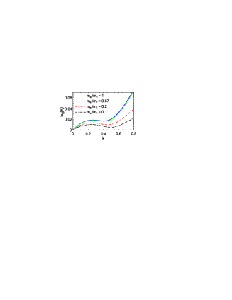
Figure 8: Modification of the dispersion curve under variation of $m_{e}/m_{h}$ ($na_{0}^{2}=0.003$, $d=5a_{0}$, $\varepsilon_{1}=\varepsilon_{2}$). The energy $E_{0}(k)$ is in units of $2Ry_{eff}$, and $k$ is in units of $a_{0}^{-1}$.

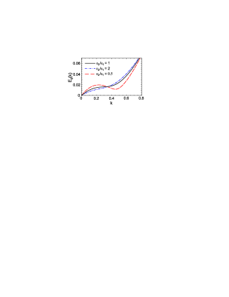
Figure 9: Modification of the dispersion curve under variation of $\varepsilon_{1}/\varepsilon_{2}$ ($na_{0}^{2}=0.002$, $d=5a_{0}$, $m_{e}=m_{h}$). The energy $E_{0}(k)$ is in units of $2Ry_{eff}$, and $k$ is in units of $a_{0}^{-1}$.

Appendix B Evaluation of the integral in Eq. (57).

The real part of the pole in the integrand in (57) is equal to $k_{\lambda}(\xi)$, the function defined implicitly by Eq. (25). The imaginary part of the pole is given by the equation

$$k^{\prime\prime}=\frac{\eta}{\left[\frac{dE_{0}(k)}{dk}-\frac{E_{0}(k)}{k}\right]\Bigg{|}_{k=k_{\lambda}(\xi)}}=\frac{\eta}{\left[v_{g0}(\xi)-v_{p0}(\xi)\right]}.$$ (88)

The integral over $k$ in (57) can be evaluated using the residue theorem. To apply this theorem we consider the contours of integration shown in Fig. 10 and labeled as $C_{+}$ and $C_{-}$. These contours include the integral along the real axis (this is the integral we are looking for), the integral along the imaginary axis and the integral along the arc $|k|=\infty$. We choose the contour $C_{+}$ or $C_{-}$ depending on the sign of $\cos(\xi-\chi)$. If $\cos(\xi-\chi)>0$ the integral along the arc is equal to zero for the contour $C_{+}$ and we choose the contour $C_{+}$. In the opposite case [$\cos(\xi-\chi)<0$] we choose the contour $C_{-}$. Under such a choice the sum of the integrals along the real and along the imaginary axes is equal to the residue of the pole if the latter is located inside the contour and it is equal to zero otherwise. Since the sign of $k^{\prime\prime}$ (88) coincides with the sign of $\left[v_{g0}(\xi)-v_{p0}(\xi)\right]$, the relevant contour encircles the pole if $\cos(\xi-\chi)$ and $\left[v_{g0}(\xi)-v_{p0}(\xi)\right]$ are of the same sign.

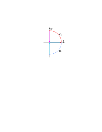
Figure 10: Contours $C_{+}$ (red) and $C_{-}$ (blue) in the $(k^{\prime},k^{\prime\prime})$ complex plane used for the calculation of the integral over $k$ in Eq. (57).

The contribution of the residue is proportional to $1/\sqrt{r}$, while the integral along the imaginary axis is proportional to $1/r^{2}$ (at $r\gg r_{0}$). We are interested in the stationary wave pattern at large distance from the obstacle. Therefore we neglect the contribution $\propto 1/r^{2}$ and equate the integral along the real axis to the residue,

$$\delta n(\mathbf{r})=\frac{nU_{0}}{\pi}\mathrm{Im}\int_{-\frac{\pi}{2}}^{\frac{\pi}{2}}d\xi\sum_{\lambda}e^{ik_{\lambda}(\xi)r\cos(\chi-\xi)}s_{\lambda}(\xi,\chi)\left[\frac{k\left[\epsilon_{k}+(\gamma_{k}^{(ex,1)}-\gamma_{k}^{(ex,2)})n\right]}{E_{0}(k)\left[\frac{dE_{0}(k)}{dk}-\frac{E_{0}(k)}{k}\right]}\right]\Bigg{|}_{k=k_{\lambda}(\xi)}.$$ (89)

The integral over $\xi$ in (89) is evaluated in the stationary phase approximation. The stationary phase condition is

$$\frac{df_{\lambda}(\xi)}{d\xi}=0,$$ (90)

where the phase $f_{\lambda}(\xi)$ is given by Eq. (59). Equation (90) implicitly defines the function $\xi_{\lambda}(\chi)$. In the general case this function is the multivalued one. We use the notation $\xi_{\lambda,i}(\chi)$, where $i$ is the branch number. One can show that the function $\xi_{\lambda}(\chi)$ is reciprocal to the function $\chi(\xi)$ defined in Sec. III (see, for instance, [52]). By expanding the phase (59) into a series near the stationary points $\xi_{\lambda,i}(\chi)$, we obtain Eq. (58).

References

- [1] G. B. Whitham, Linear and Nonlinear Waves (New York: Wiley-Interscience, 1974).
-
[2]
E. Cornell. Talk at the KITP Conference on Quantum Gases (2004)
[ http://online.itp.ucsb.edu/online/gases_c04/cornell/].
- [3] I. Carusotto, S. X. Hu, L. F. Collins, and A. Smerzi, Bogoliubov-Cerenkov Radiation in a Bose-Einstein Condensate Flowing against an Obstacle, Phys. Rev. Lett. 97, 260403 (2006).
- [4] Yu. G. Gladush, G. A. El, A. Gammal, and A. M. Kamchatnov, Radiation of linear waves in the stationary flow of a Bose-Einstein condensate past an obstacle, Phys. Rev. A 75, 033619 (2007).
- [5] Yu. G. Gladush, L. A. Smirnov, and A. M. Kamchatnov, Generation of Cherenkov waves in the flow of a Bose-Einstein condensate past an obstacle, J. Phys. B: At. Mol. Opt. Phys. 41, 165301 (2008).
- [6] T.-L. Horng, S.-C. Gou, T.-C. Lin, G. A. El, A. P. Itin, and A. M. Kamchatnov, Stationary wave patterns generated by an impurity moving with supersonic velocity through a Bose-Einstein condensate, Phys. Rev. A 79, 053619 (2009).
- [7] F. Ursell, On Kelvin’s ship-wave pattern, Journal of Fluid Mechanics 8, 418, (1960).
- [8] Yu. G. Gladush, A. M. Kamchatnov, Z. Shi, P. G. Kevrekidis, D. J. Frantzeskakis, and B. A. Malomed, Wave patterns generated by a supersonic moving body in a binary Bose-Einstein condensate, Phys. Rev. A 79, 033623 (2009).
- [9] L.Y. Kravchenko and D.V. Fil, Stationary Waves in a Supersonic Flow of a Two-Component Bose Gas, J. Low Temp. Phys. 155, 219 (2009).
- [10] A. Amo, L. Jerome, P. Simon, C. Adrados, C. Ciuti, I, Carusotto, R. Houdre, E. Giacobino and A. Bramati, Superfluidity of polaritons in semiconductor microcavities, Nature Phys. 5, 805 (2009).
- [11] I. Carusotto and C. Ciuti, Quantum fluids of light, Rev. Mod. Phys. 85, 299 (2013).
- [12] P. Cilibrizzi, H. Ohadi, T. Ostatnicky, A. Askitopoulos, W. Langbein, and P. Lagoudakis, Linear Wave Dynamics Explains Observations Attributed to Dark Solitons in a Polariton Quantum Fluid, Phys. Rev. Lett. 113, 103901 (2014).
- [13] A. M. Kamchatnov and N. Pavloff, Interference effects in the two-dimensional scattering of microcavity polaritons by an obstacle: Phase dislocations and resonances, Eur. Phys. J. D 69, 32 (2015).
- [14] E. Cancellieri, F. M. Marchetti, M. H. Szymanska, and C. Tejedor, Superflow of resonantly driven polaritons against a defect, Phys. Rev. B 82, 224512 (2010).
- [15] G. Lerario, A. Fieramosca, F. Barachati, D. Ballarini, K. S. Daskalakis, L. Dominici, M. De Giorgi, S. A. Maier, G. Gigli, S. Kena-Cohen and D. Sanvitto, Room-temperature superfluidity in a polariton condensate, Nature Phys. 13, 837 (2017).
- [16] S. I. Shevchenko, Theory of superconductivity of systems with pairing of spatially separated electrons and holes, Fiz. Nizk. Temp. 2, 505 1976 [Sov. J. Low Temp. Phys., 2, 251 (1976)].
- [17] Yu. E. Lozovik and V. I. Yudson, A new mechanism for superconductivity: Pairing between spatially separated electrons and holes, Zh. Eksp. Teor. Fiz. 71, 738 (1976) [ Sov. Phys. JETP 44, 389 (1976)].
- [18] A. I. Bezuglyi and S. I. Shevchenko, Effect of Impurities on Thermodynamic and Kinetic Properties of Systems with Electron-Hole Pairing, Fiz. Nizk. Temp. 3, 428 (1977) [Sov. J. Low Temp. Phys. 3, 203 (1977)].
- [19] K. V. Germash and D. V. Fil, Electromagnetic properties of a double-layer graphene system with electron-hole pairing, Phys. Rev. B 93, 205436 (2016).
- [20] K. V. Germash and D. V. Fil, Anderson-Bogoliubov and Carlson-Goldman modes in counterflow superconductors: Case study of a double monolayer graphene, Phys. Rev. B 99, 125412 (2019).
- [21] J. R. Schrieffer, Theory of Superconductivity (Benjamin, New York, 1964).
- [22] L. V. Keldysh, ”Coherent states of excitons,” in Problems of Theoretical Physics. In Memory of Igor Evgenievich Tamm, edited by V. I. Ritus (Nauka, Moscow, 1972), p. 433; Phys. Usp. 87, 1273 (2017).
- [23] P. B. Littlewood, Exciton coherence, in Problems of Condensed Matter Physics: Quantum coherence phenomena in electron-hole and coupled matter-light systems, edited by A. L. Ivanov and A. M. Tikhodeev (Oxford University Press, New-York, 2008).
- [24] D. V. Fil and S. I. Shevchenko, Superfluidity of a dilute gas of electron-hole pairs in a bilayer system, Fiz. Nizk. Temp. 42, 1013 (2016) [Low Temp. Phys. 42, 794 (2016)].
- [25] D. V. Fil and S. I. Shevchenko, Electron-hole Superconductivity (Review), Fiz. Nizk. Temp. 44, 1111 (2018) [Low Temp. Phys. 44, 867 (2018)].
- [26] H. A. Fertig, Energy spectrum of a layered system in a strong magnetic field, Phys. Rev. B 40, 1087 (1989).
- [27] D. Yoshioka and A. H. MacDonald, Double Quantum Well Electron-Hole Systems in Strong Magnetic Fields. J. Phys. Soc. Jpn. 59, 4211 (1990).
- [28] K. Moon, H. Mori, K. Yang, S. M. Girvin, A. H. MacDonald, L. Zheng, D. Yoshioka, and S. C. Zhang, Spontaneous interlayer coherence in double-layer quantum Hall systems: Charged vortices and Kosterlitz-Thouless phase transitions, Phys. Rev. B 51, 5138 (1995).
- [29] M. Kellogg, J. P. Eisenstein, L. N. Pfeiffer, and K. W. West, Vanishing Hall Resistance at High Magnetic Field in a Double-Layer Two-Dimensional Electron System, Phys. Rev. Lett. 93, 036801 (2004).
- [30] E. Tutuc, M. Shayegan, and D. A. Huse, Counterflow Measurements in Strongly Correlated GaAs Hole Bilayers: Evidence for Electron-Hole Pairing, Phys. Rev. Lett. 93, 036802 (2004).
- [31] R. D. Wiersma, J. G. S. Lok, S. Kraus, W. Dietsche, K. von Klitzing, D. Schuh, M. Bidder, H. - P. Tranitz, and W. Wegscheider, Activated Transport in the Separate Layers that Form the Exciton Condensate, Phys. Rev. Lett. 93, 266805 (2004).
- [32] D. Nandi, A. D. K. Finck, J. P. Eisenstein, L. N. Pfeiffer, and K. W. West, Exciton condensation and perfect Coulomb drag, Nature (London), 488, 481 (2012).
- [33] J. P. Eisenstein, Exciton Condensation in Bilayer Quantum Hall Systems, Ann. Rev. Condensed Matter Phys. 5, 159 (2014).
- [34] A. F. Croxall, K. Das Gupta, C. A. Nicoll, M. Thangaraj, H. E. Beere, I. Farrer, D. A. Ritchie, and M. Pepper, Anomalous Coulomb Drag in Electron-Hole Bilayers, Phys. Rev. Lett., 101, 246801 (2008).
- [35] J. A. Seamons, C. P. Morath, J. L. Reno, and M. P. Lilly, Coulomb Drag in the Exciton Regime in Electron-Hole Bilayers, Phys. Rev. Lett. 102, 026804 (2009).
- [36] H. Min, R. Bistritzer, J.-J. Su, and A. H. MacDonald, Room-temperature superfluidity in graphene bilayers. Phys. Rev. B 78, 121401(R) (2008).
- [37] Yu. E. Lozovik and A. A. Sokolik, Coherent phases and collective electron phenomena in graphene, J. Phys.: Conf. Ser. 129, 012003 (2008).
- [38] A. Perali, D. Neilson, and A. R. Hamilton, High-Temperature Superfluidity in Double-Bilayer Graphene, Phys. Rev. Lett. 110, 146803 (2013).
- [39] I. Sodemann, D. A. Pesin, and A. H. MacDonald, Interaction-enhanced coherence between two-dimensional Dirac layers, Phys. Rev. B 85, 195136 (2012).
- [40] S. Conti, A. Perali, F. M. Peeters, and D. Neilson, Multicomponent screening and superfluidity in gapped electron-hole double bilayer graphene with realistic bands, Phys. Rev. B 99, 144517 (2019).
- [41] G. W. Burg, N. Prasad, K. Kim, T. Taniguchi, K. Watanabe, A. H. MacDonald, L. F. Register, and E. Tutuc, Strongly Enhanced Tunneling at Total Charge Neutrality in Double-Bilayer Graphene- WSe2 Heterostructures, Phys. Rev. Lett. 120, 177702 (2018).
- [42] D. K. Efimkin, G. W. Burg, E. Tutuc, and A. H. MacDonald, Tunneling and fluctuating electron-hole Cooper pairs in double bilayer graphene, Phys. Rev. B 101, 035413 (2020).
- [43] S. Saberi-Pouya, S. Conti, A. Perali, A. F. Croxall, A. R. Hamilton, F. M. Peeters, and D. Neilson, Experimental conditions for the observation of electron-hole superfluidity in GaAs heterostructures, Phys. Rev. B 101, 140501(R) (2020).
- [44] F. C. Wu, F. Xue, and A. H. MacDonald, Theory of two-dimensional spatially indirect equilibrium exciton condensates, Phys. Rev. B 92, 165121 (2015).
- [45] O. L. Berman and R. Ya. Kezerashvili, High-temperature superfluidity of the two-component Bose gas in a transition metal dichalcogenide bilayer, Phys. Rev. B 93, 245410 (2016).
- [46] O. L. Berman and R. Ya. Kezerashvili, Superfluidity of dipolar excitons in a transition metal dichalcogenide double layer, Phys. Rev. B, 96, 094502 (2017).
- [47] B. Debnath, Y. Barlas, D. Wickramaratne, M. R. Neupane, and R. K. Lake, Phys. Rev. B, Exciton condensate in bilayer transition metal dichalcogenides: Strong coupling regime, 96, 174504 (2017).
- [48] M. Van der Donck and F. M. Peeters, Interlayer excitons in transition metal dichalcogenide heterostructures, Phys. Rev. B 98, 115104 (2018).
- [49] M. Xie and A. H. MacDonald, Electrical Reservoirs for Bilayer Excitons, Phys. Rev. Lett. 121, 067702 (2018).
- [50] S. Conti, D. Neilson, F. M Peeters, and A. Perali, Transition Metal Dichalcogenides as Strategy for High Temperature Electron-Hole Superfluidity, Condens. Matter 5, 22 (2020).
- [51] Z. Wang, D. A. Rhodes, K. Watanabe, T. Taniguchi, J. C. Hone, J. Shan, and K. F. Mak, Evidence of high-temperature exciton condensation in two-dimensional atomic double layers, Nature 574, 76 (2019).
- [52] A. A. Pikalov and D. V. Fil, Stationary waves in a superfluid exciton gas in quantum Hall bilayers, J. Phys.: Condens. Matter 23, 265301 (2011).
- [53] M. Abolfath, A. H. MacDonald, and L. Radzihovsky, Critical currents of ideal quantum Hall superfluids, Phys. Rev. B 68, 155318 (2003).
- [54] L. Yu. Kravchenko and D. V. Fil, Critical currents and giant non-dissipative drag for superfluid electron-hole pairs in quantum Hall multilayers, J. Phys.: Condens. Matter 20, 325235 (2008).
- [55] D. V. Fil and L. Yu. Kravchenko, Superconductivity of electron-hole pairs in a bilayer graphene system in a quantizing magnetic field, Fiz. Nizk. Temp. 35, 904 (2009) [Low Temp. Phys. 35, 712 (2009)].
- [56] D. V. Fil and S. I. Shevchenko, Transition to a supersolid phase in a two-dimensional dilute gas of electron-hole pairs, Fiz. Nizk. Temp. 46, 556 (2020) [Low Temp. Phys. 46, 465 (2020)].
- [57] Yogesh N. Joglekar, Alexander V. Balatsky, and S. Das Sarma, Wigner supersolid of excitons in electron-hole bilayers, Phys. Rev. B 74, 233302 (2006).
- [58] Jinwu Ye, Quantum Phases of Excitons and Their Detections in Electron-Hole Semiconductor Bilayer Systems, Journal of Low Temperature Physics 158, 882 (2010).
- [59] I. L. Kurbakov, Yu. E. Lozovik, G. E. Astrakharchik, and J. Boronat, Quasiequilibrium supersolid phase of a two-dimensional dipolar crystal, Phys. Rev. B 82, 014508 (2010).
- [60] Z.-K. Lu, Y. Li, D. S. Petrov, and G. V. Shlyapnikov, Stable dilute supersolid of two-dimensional dipolar bosons, Phys. Rev. Lett. 115, 075303 (2015).
- [61] L. Tanzi, E. Lucioni, F. Fama, J. Catani, A. Fioretti, C. Gabbanini, R.N. Bisset, L. Santos, and G. Modugno, Observation of a Dipolar Quantum Gas with Metastable Supersolid Properties, Phys. Rev. Lett. 122, 130405 (2019).
- [62] Fabian Bottcher, Jan-Niklas Schmidt, Matthias Wenzel, Jens Hertkorn, Mingyang Guo, Tim Langen, and Tilman Pfau, Transient Supersolid Properties in an Array of Dipolar Quantum Droplets, Phys. Rev. X 9, 011051 (2019).
- [63] L. Chomaz, D. Petter, P. Ilzhofer, G. Natale, A. Trautmann, C. Politi, G. Durastante, R.M.W. van Bijnen, A. Patscheider, M. Sohmen, M.J. Mark, and F. Ferlaino, Long-Lived and Transient Supersolid Behaviors in Dipolar Quantum Gases, Phys. Rev. X 9, 021012 (2019).
- [64] S. I. Shevchenko and A. S. Rukin, On electrical phenomena in electroneutral superfluid systems, Fiz. Nizk. Temp. 36, 186 (2010) [Low Temp. Phys. 36, 146 (2010)].
- [65] S. I. Shevchenko and A. S. Rukin, Two approaches to the description of dilute superfluid Bose systems, Fiz. Nizk. Temp. 38, 1147 (2012) [Low Temp. Phys. 38, 905 (2012)].
- [66] Camille Lagoin, Stephan Suffit, Kenneth West, Kirk Baldwin, Loren Pfeiffer, Markus Holzmann, and Francois Dubin, Quasicondensation of Bilayer Excitons in a Periodic Potential, Phys. Rev. Lett. 126, 067404 (2021).
- [67] Luiz H. G. Tizei, Yung-Chang Lin, Masaki Mukai, Hidetaka Sawada, Ang-Yu Lu, Lain-Jong Li, Koji Kimoto, and Kazu Suenaga, Exciton Mapping at Subwavelength Scales in Two-Dimensional Materials, Phys. Rev. Lett. 114, 107601 (2015).
- [68] J. Martin, N. Akerman, G. Ulbricht, T. Lohmann, J. H. Smet, K. von Klitzing, and A. Yacoby, Observation of electron-hole puddles in graphene using a scanning single-electron transistor, Nature Physics 4, 144 (2008).