MODELLING AND SIMULATIONS OF ELECTRICAL PROPAGATION IN TRANSMURAL SLABS OF SCARRED LEFT VENTRICULAR TISSUE

Abstract

We report three-dimensional and time-dependent numerical simulations of the propagation of electrical action potentials in a model of rabbit ventricular tissue. The simulations are performed using a finite-element method for the solution of the monodomain equations of cardiac electrical excitation. The parameters of a detailed ionic ventricular cell model are re-fitted to available experimental data and the model is then used for the description of the transmembrane current and calcium dynamics. A region with reduced conductivity is introduced to model a myocardial infarction scar. Electrical activation times and density maps of the transmembrane voltage are computed and compared with experimental measurements in rabbit preparations with myocardial infarction obtained by a panoramic optical mapping method.

Mortensen, Noor Aziz, Gao and Simitev

1 INTRODUCTION

The heartbeat is controlled by a particular pattern of an electrical wave. When the heart is damaged by a myocardial infarction (MI), this pattern is disturbed, leading to arrhythmias and heart failure. Thus, it is important to understand how this pattern is formed and how MI scars affect it. Here we begin to explore these effects by mathematical modelling and simulation of action potential propagation in a slab of cardiac tissue, based on and compared to experiments performed on post MI rabbit hearts.

2 MATHEMATICAL MODEL

2.1 Tissue model

We consider the monodomain model given by the set of equations

$$\chi C_{m}\frac{\partial V}{\partial t}-\nabla\cdot(\bm{\mathrm{\sigma}}\nabla V)=-\chi\,I_{\text{ion}}-\chi\,I_{\text{stim}}(\bm{\mathrm{x}},t),$$ (1a)

$$I_{\text{ion}}=I_{\text{ion}}\big{(}V(\bm{\mathrm{x}},t),\bm{\mathrm{y}}(\bm{\mathrm{x}},t)\big{)},$$ (1b)

$$\frac{\partial\bm{\mathrm{y}}}{\partial t}=\bm{\mathrm{R}}\big{(}V,\bm{\mathrm{y}}\big{)},$$ (1c)

$$\text{for }\quad\bm{\mathrm{x}}\in\Omega,\quad t\in[0,\infty),$$ (1d)

with boundary conditions

$$\frac{\partial V}{\partial\bm{\mathrm{n}}}=0\quad\text{on }\quad\bm{\mathrm{x}}\in\partial\Omega,$$ (1e)

in a spacial domain $\Omega\in\mathbb{R}^{3}$ representing a piece of cardiac tissue with $\bm{\mathrm{n}}$ being the outer normal unit vector to its boundary $\partial\Omega$. Here $V$ is the cardiac transmembrane electric voltage potential measured in mV, $I_{\text{ion}}$ is electric current density across the membrane of cardiomyocyte cells measured in $\mu\text{A mm}^{-2}$, $I_{\text{stim}}$ is the density of an externally applied stimulus current also measured in $\mu\text{A mm}^{-2}$, $\chi$ is the surface-to-volume ratio of cardiomyocytes measured in $\text{mm}^{-1}$, $\bm{\mathrm{\sigma}}$ is the effective conductivity of the cardiac tissue measured in $\text{mS mm}^{-1}$ and $C_{m}$ is the specific cell membrane capacitance measured in $\mu\text{F mm}^{-2}$. The transmembrane current $I_{\text{ion}}$ is modelled as a function of a vector of state variables $\bm{\mathrm{y}}$ representing ionic concentrations and ionic channel gating variables determined by a system of nonlinear ordinary differential equations with rates given by $\bm{\mathrm{R}}$. The monodomain model provides a biophysical continuum representation of cardiac electrophysiology in both space and time, linking tissue-scale electrical propagation with cellular electrical excitation. The monodomain equations are derived from the laws of conservation of charge and the assumption that infinitesimal pieces of the cardiomyocyte membrane may be modelled as an circuit of a conductor and capacitor connected in parallel.

Specific values for $\sigma$, $C_{m}$ and $\chi$ as well as for the geometry of the tissue used are given further below.

2.2 Single-cell electrophysiology models

A large number of single-cell ionic current models given by equations (1b) and (1c) of the monodomain system (1) exist to represent the conducting properties of cardiac myocyte membranes. These models can be classified into conceptual and detailed with the detailed ionic models further divided into models for various type cells (atrial, ventricular, sino-atrial, Purkinje), various species (human, porcine, canine, leporine, murine) and various state of remodelling (healthy normal, in heart failure etc.) These models are subject to continuous re-evaluation and refinement as new experimental data becomes available. The contemporary models include tens of ordinary differential equations and online model repositories such as CellML have been setup for ease of their dissemination and use.

Details of the specific single-cell ionic current models we use are provided further below.

3 NUMERICAL METHODS OF SOLUTION

3.1 Operator splitting

The monodomain model (1) is characterised by a large range of significant scales, e.g. cardiac action potentials have extremely fast and narrow upstrokes (depolarization) and very slow and bread recovery (repolarization) phases. An effective numerical scheme based on an operator splitting approach (Godunov and Strang splitting, [15], also known as the fractional timestep method [13]), was proposed by Qu and Garfinkel [14] and is adopted in our study in the following form. The nonlinear monodomain model (1) is split into a set of nonlinear ordinary differential equations

$$\frac{\partial V}{\partial t} =-\frac{1}{C_{m}}\big{(}I_{\text{ion}}(V,\bm{\mathrm{y}})+I_{\text{stim}}\big{)},$$

$$\frac{\partial\bm{\mathrm{y}}}{\partial t} =\bm{\mathrm{R}}\big{(}V,\bm{\mathrm{y}}\big{)},$$ (2a)

and a linear diffusion partial differential equation

$$\frac{\partial V}{\partial t} =\frac{1}{\chi C_{m}}\nabla\cdot(\bm{\mathrm{\sigma}}\nabla V).$$ (2b)

To integrate the complete monodomain model (1) in the interval $[t_{n},t_{n}+\Delta t]$ we take the following three fractional steps of the splitting algorithm.

1. Solve the nonlinear ODE system for $V_{\theta}^{n}$ at $t_{n}<t\leq t_{n}+\theta\Delta t$ with known $V^{n}$

   $$\frac{\partial V}{\partial t}=-\frac{1}{C_{m}}I_{\text{ion}}(V,\bm{\mathrm{y}}),\qquad\frac{\partial\bm{\mathrm{y}}}{\partial t}=\bm{\mathrm{R}}(V,\bm{\mathrm{y}}),\qquad V(t_{n})=V^{n}.$$

2. Solve the linear PDE for $V_{\theta}^{n+1}$ at $t_{n}<t\leq t_{n}+\Delta t$

   $$\frac{\partial V}{\partial t}=\frac{1}{\chi C_{m}}\nabla\cdot(\bm{\mathrm{\sigma}}\nabla V),\quad\quad V(t_{n})=V_{\theta}^{n}.$$

3. Solve the ODE system again for $V^{n+1}$ at $t_{n}+\theta\Delta t<t\leq t_{n}+\Delta t$

   $$\frac{\partial V}{\partial t}=-\frac{1}{C_{m}}I_{\text{ion}}(V,\bm{\mathrm{y}}),\qquad\frac{\partial\bm{\mathrm{y}}}{\partial t}=\bm{\mathrm{R}}(V,\bm{\mathrm{y}}),\qquad V(t_{n}+\theta\Delta t)=V_{\theta}^{n+1}.$$

Further details on the operator splitting method applied to the monodomain problem can be found in [16].

3.2 Reaction part

In this form the normally stiff initial value problem (2a) can be integrated separately using one of the many known methods for solution of initial value problems, including adaptive time stepping. Depending on the specific ionic models, a forward Euler method may be used for temporal stepping for less stiff cases, or a fourth-order Runge-Kutta method, for stiffer problems, for instance.

3.3 Diffusion part

The diffusion part of the monodomain model (1) is solved using a finite-element method as detailed below. For the spacial disretisation of the equation (2b) the numerical approximation $V^{h}(\bm{\mathrm{x}},t)$ of the transmembrane voltage potential $V(\bm{\mathrm{x}},t)$ is assumed to take the form of a finite expansion in a set of continuous piecewise polynomial nodal basis functions $\big{\{}\phi^{h}_{i}(\bm{\mathrm{x}}),i=1..p\big{\}}$ with time-dependent coefficients $\big{\{}V_{i}(t),i=1..p\big{\}}$ each representing a nodal value at time $t$

$$V(\bm{\mathrm{x}},t)\approx V^{h}(\bm{\mathrm{x}},t)=\sum_{i=1}^{p}\phi_{i}(\bm{\mathrm{x}})V_{i}(t),$$ (3)

where $p=\dim\{\phi^{h}\}$, and $h$ denotes a parameter measuring the size of the domain partition. Substituting expansion (3) in equation (1a), taking the Galerkin projection and using the boundary condition (1e), the following weak variational form of the monodomain equation is obtained

$$\chi\,C_{m}\Big{(}\frac{\partial V^{h}}{\partial t},\phi^{h}_{i}\Big{)}_{\Omega}+\Big{(}\bm{\mathrm{\sigma}}\nabla V^{h},\nabla\phi^{h}_{i}\Big{)}_{\Omega}=0,$$ (4)

$$\quad i=1,\dots,p,$$

representing a weighted-residual condition for minimization of the residual error, where the round brackets $(v,w)_{\Omega}=\int_{\Omega}vw\,d\Omega$ denote the inner product with the basis functions. The Galerkin approximaiton (4) represents a set of $p$ ordinary differential equations in time for the $p$ coefficient functions $V_{i}(t)$ in the expansion (3). For brevity in the following we will drop the superscript $h$.

For the temporal disretisation of the Galerkin projection equations (4) the time derivative approximated a first-order accurate forward finite difference formula and the following implicit numerical scheme is used

$$\chi\,C_{m}\,\bm{\mathrm{M}}\frac{\bm{\mathrm{V}}^{n+1}-\bm{\mathrm{V}}^{n}}{\Delta t}+\bm{\mathrm{K}}\,\bm{\mathrm{V}}^{n+1}=0,$$ (5)

where $\bm{\mathrm{V}}^{n}=[V_{1}^{n},V_{2}^{n},\dots,V_{p}^{n}]^{T}$ now denotes $p$-dimensional vector of voltage values at time level $t_{n}=n\Delta t$ with time step $\Delta t$, and where

$$[M_{ij}]=(\phi_{i},\phi_{j})_{\Omega},$$

denotes the mass matrix and

$$[K_{ij}]=(\nabla\phi_{i},\bm{\mathrm{\sigma}}\nabla\phi_{j})_{\Omega},$$

denotes the stiffness matrix. Finally, the vector of unknowns voltage values at time level $t_{n+1}$ is determined by solving the linear system of equations

$$(\bm{\mathrm{M}}+\frac{\Delta t}{\chi\,C_{m}}\,\bm{\mathrm{K}})\,\bm{\mathrm{V}}^{n+1}=\bm{\mathrm{M}}\,\bm{\mathrm{V}}^{n}.$$ (6)

3.4 Practical implementation

Equation (6) is solved using the libMesh open source parallel C++ finite element library [5], and the solution of linear systems and the time stepping relies on the solvers provided by the PETSc library. Simulations are run both on our local Linux workstations with 2 Intel(R) Xeon (R) CPU E5-2699 2.30 GHz (up to 72 threads) and 128 GB of memory at the School of Mathematics and Statistics, University of Glasgow as well as on the RCUK flagship High-Performance parallel computer ARCHER. Visit is used for post-processing the two- and three-dimensional simulations.

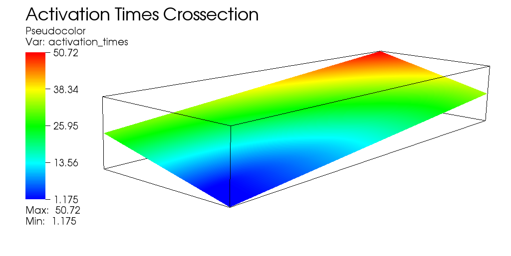
Figure 1: Computational domain A contour plot of activation times for the benchmark problem defined in section 4. The computational domain is clearly visible. The stimulus site is in the lower central vertex while the most distant point is the upper central vertex.

		$\Delta x$
		0.5mm	0.333mm	0.2mm	0.1mm
$\Delta t$	0.05ms	81.75	60.95	52.15	47.20
	0.025ms	80.70	59.85	49.94	45.40
	0.01ms	80.06	59.20	49.94	44.26
	0.005ms	79.82	58.96	49.65	43.85

Table 1: Values for the activation time [ms] at different spatial and temporal discretisation steps measured in our numerical code for the benchmark problem described in section 4.

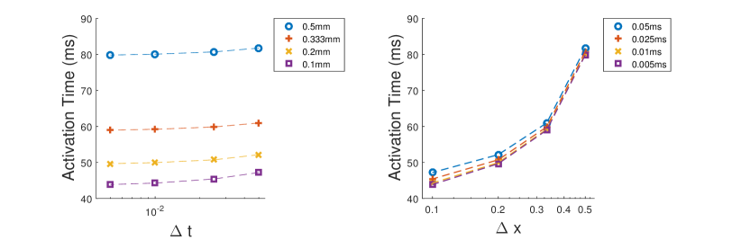
Figure 2: Convergence of the value of the activation time as time and space steps are decreased. Values are measured in our numerical code for the benchmark problem described in section 4.

4 BENCHMARKING AND VALIDATION

4.1 Benchmark description

Our mathematical model and its numerical implementation was validated by comparison with a standard cardiac tissue electrophysiology simulation benchmark case developed by the research community [12]. The benchmark involved 11 independently developed numerical codes providing numerical simulations of a well-defined problem with unique solution for a number of different resolutions. The benchmark seeks to compare solutions of the monodomain equations (1) on a cuboid domain of dimensions $20\times 7\times 3$ mm using the ten Tusscher and Panfilov [17] model of human epicardial myocytes as a model of the transmembrane ion current density $I_{\text{ion}}$. The initial stimulus current $I_{\text{stim}}$ has a current density amplitude of $50000\mu\text{A cm}^{-3}$ and is applied to a cube with size $1.5\times 1.5\times 1.5$ mm positioned at the corner of the full cuboid domain and a stimulus duration of 2 ms. The value of the cell surface to volume ratio $\chi$ is 140 mm^-1, and it is assumed that the cardiac fibres are aligned with the long, 20 mm, axis of the cuboid domain so the conductivity tensor $\bm{\mathrm{\sigma}}$ is diagonal with values $[0.1334,0.0176,0.0176]$ S m^-1 along its main diagonal. The so called “activation time” defined as the time it takes for a cardiac action potential to travel from the stimulation site to the most distant point in the computational domain (i.e. the point opposite the stimulation site) is requested as a diagnostic output quantity from the numerical simulation. Figure 1 shows the geometry of the benchmark case.

4.2 Validation and benchmarking

We have verified that our numerical code is in excellent agreement with the community benchmark results. Since the computational domain of the benchmark problem is rectangular domain we have used a regular square finite-element mesh with space step $\Delta x$. For time stepping we have used the simple forward Euler method with time step $\Delta t$. Table 1 shows the values of the activation time we have obtained at various spatial and temporal resolutions. At the highest resolution of $\Delta x=0.1$ mm and $\Delta t=10^{-4}$ ms the activation time obtained using our code is $43.85$ ms which is within 2% error bar from the 42.82 ms high-accuracy value agreed upon in the benchmark paper [12]. Figure 2 shows a convergence test we have performed with decreasing space step and time step and it is clear that our solution is converging to values closer to the community benchmark value just quoted. We remark that for our code the increase of the spatial resolution leads to more significant increases of accuracy than the increase in temporal resolution.

Parameters	M-cells (Healthy)	M-cells (MI)
$K_{0}$, External potassium concentration (mM)	4.5865	4.3087
$Ca_{0}$, External calcium concentration (mM)	2.0467	2.5678
$Na_{0}$, External sodium concentration (mM)	146.30	165.71
$gna$, Peak INa conductance	14	12
$gca$, Strength of Ca current flux (mmol/(cm C))	259.86	193.23
$pca$, Constant in ICal (cm/s)	0.0002	0.0008
$r1$, Opening rate in ICal	0.4804	0.3546
$r2$, Closing rate in ICal	2.2825	2.8694
$gkix$, Peak IK1 conductance (mS/$\mu$F)	0.4400	0.2604
$gtof$, Peak Ito conductance (mS/$\mu$F)	0.0221	0.0421
(Global) root mean square error	0.0133	0.1070

Table 2: Parameter values of the model of Mahajan et al. [7] re-fitted to the experimental data on M-cells at 3 Hz pacing rate form [8].

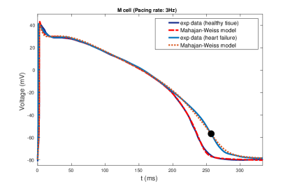
Figure 3: Action potential computed using the model of Mahajan et al. [7] with parameter values given in table 2 in comparison with experimental data from [8].

5 PARAMETER RE-FITTING OF A RABBIT VENTRICULAR SINGLE CELL IONIC MODEL

In order to achieve an accurate comparison with experimental measurements in rabbit ventricular tissue samples e.g. [1, 11, 10] an appropriate single cell ionic action potential model must be selected and refitted. To this end we have selected to use Mahajan et al. [7] detailed action potential model, one of the modern rabbit ventricular AP models designed to accurately reproduce the dynamics of the cardiac action potential and intracellular calcium (Cai) cycling at rapid heart rates as relevant to ventricular tachycardia and fibrillation. Cardiac electrophysiology models are based on experimental data from a variety of sources, including measurements in different species and under different experimental conditions [3]. Refitting of model parameters is therefore necessary whenever new or more appropriate data sets are available. In our case, the model of Mahajan et al. [7] was refitted to match the single cell experimental data of McIntosh et al. [8] since these were measured by the same research group using identical experimental protocols.

In [8] action potential and intracellular Ca2+ transient characteristics $x_{i}^{\text{target}}$ were measured in single cardiac myocytes from mid-myocardial regions of the left ventricle of rabbits with and without heart failure. These were fitted to the outputs of the model of Mahajan et al. [7], $x_{i}^{\text{sim}}$, by minimising the error function

$$\text{Err}_{\text{AP}}=\frac{1}{M}\sum_{i=1}^{M}(x_{i}^{\text{sim}}-x_{i}^{\text{target}})^{2}$$ (7)

with respect to selected parameter values, aka “parameter estimation”. For parameter estimation we used a standard Matlab routine for unconstrained multivariable minimisation based on the bounded Nelder-Mead simplex-like method [6]. The results are shown in Table 2 and figure 3 below.

		$\Delta x$
		0.5mm	0.333mm	0.2mm	0.1mm
$\Delta t$	0.05ms	X	X	X	X
	0.01ms	X	X	X	54.19
	0.005ms	X	X	63.94	53.90
	0.0025ms	X	82.30	63.81	53.76
	0.0001ms	X	82.25	63.75	53.68

Table 3: Values for the activation time [ms] at different spatial and temporal discretisation steps measured in our numerical code for the benchmark geometry described in section 4 but for the model of Mahajan et al. [7] refitted to healthy values rather than ten Tusscher and Panfilov [17] model.

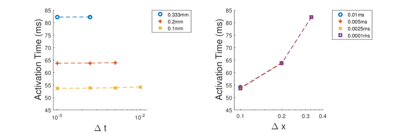
Figure 4: Convergence of the value of the activation time as time and space steps are decreased. Values are measured in our numerical code for the benchmark problem described in section 4 with the model of Mahajan et al. [7] refitted to healthy values.

The benchmark convergence test of section 4 was repeated using the model of Mahajan et al. [7] newly re-fitted to healthy values in order to establish suitable resolution. Based on the results of Table 3 and figure 4 we determine that $\Delta x=0.1$ and $\Delta t=5\times 10^{-3}$ ms provides a good trade-off between resolution and model accuracy and we use this values for the simulations detailed in the next section.

6 MODELLING OF PROPAGATION IN SCARRED TRANSMURAL VENTRICULAR SLABS

a)	b)
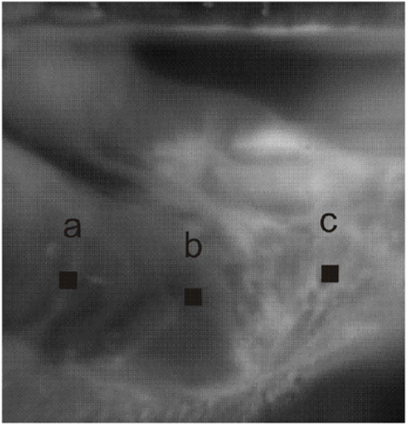
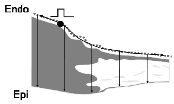
c)	d)

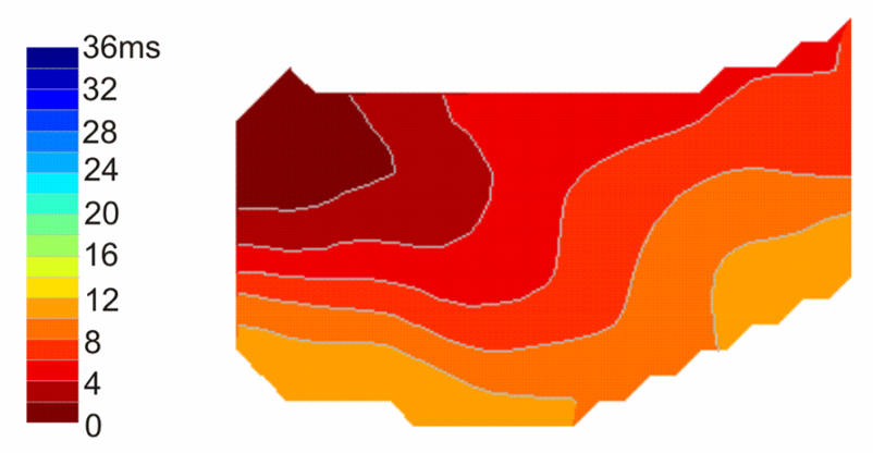
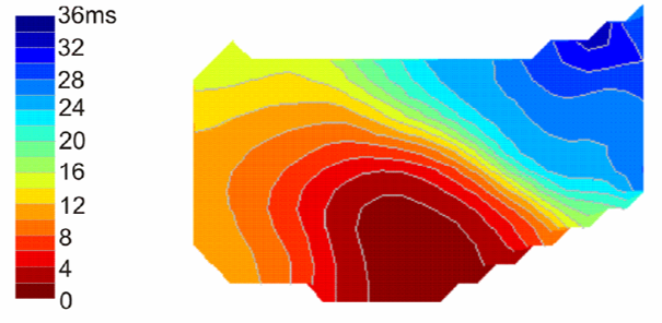
Figure 5: Transmural conduction into an infarct zone. Plots taken from figure 5.8 of [10].

(a)	(b)

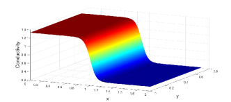
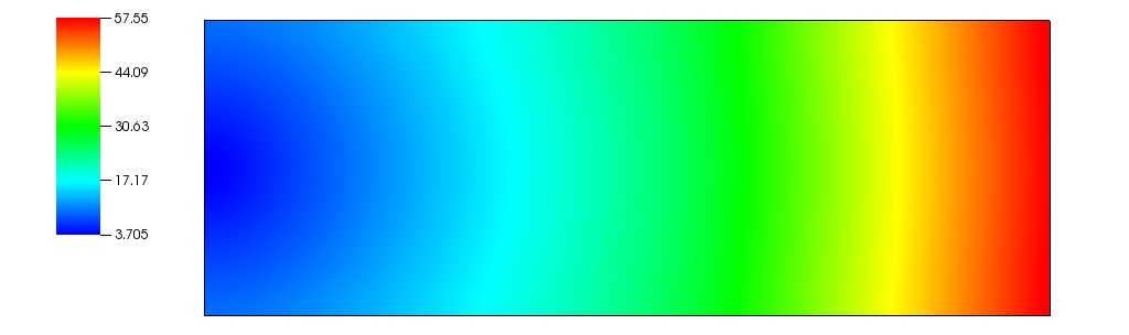
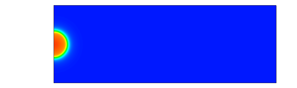
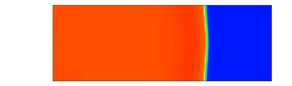
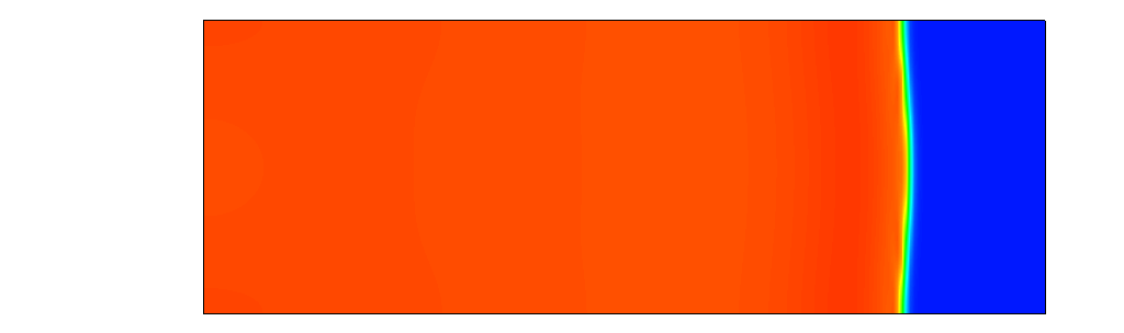
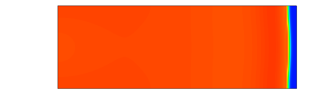
Figure 6: (a) Isotropic conductivity as a function of $x$ as given by equation (8). (b) Simulated activation times [ms] for the conductivity profile in part (a).

Figure 7: Propagation of an action potential in the case of sigmoidal conductivity (8). Density maps of the transmembrane voltage potential are plotted at equidistant times $t_{i}=5+i\Delta t$, $i=1,\dots,6$ and $\Delta t=10$ ms.

(a)	(b)

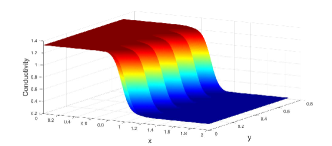
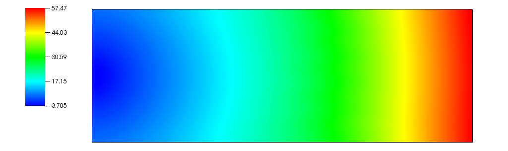
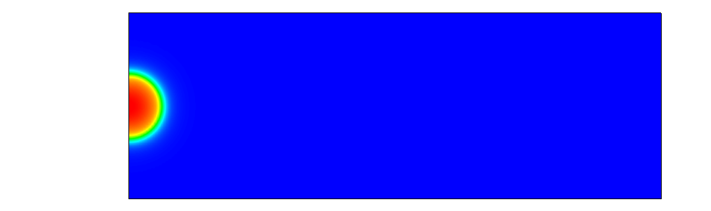
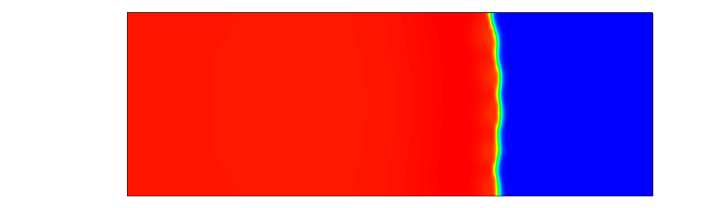
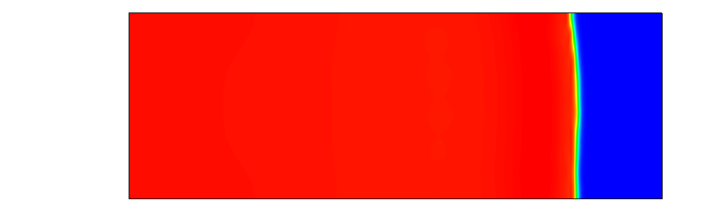
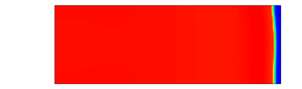
Figure 8: (a) Isotropic conductivity with a fingering effect as a function of $x$ and $y$ as given by equation (9). (b) Simulated activation times [ms] for the conductivity profile in part (a).

Figure 9: Propagation of an action potential in the case of finger-like conductivity (9). Density maps of the transmembrane voltage potential are plotted at equidistant times $t_{i}=5+i\Delta t$, $i=1,\dots,6$ and $\Delta t=10$ ms.

6.1 Physiology of the infarcted zone

6.2 Description of experiments

An example of the experimental measurements of transmural conduction into an infarct zone available from our collaborators [10] is shown in Figure 5. The upper left panel shows a plain image of the transmural surface of a wedge preparation from a ligated heart, with the endocardium uppermost and the epicardium at the bottom of the picture. The black squares indicate the position from which example APs are available for comparison: a) remote zone b) border zone and c) infarct zone. In the upper right panel is a schematic diagram of the preparation, indicating the position and the shape of the infarct border zone. The lower two panels show isochronal maps of activation time during endocardial and epicardial stimulation at left and right panels, respectively. The experiment has a number of notable features, including,

a)

The infarct zone has lower density of electrically excitable cells.

b)

The infarct border zone has significant undulations that protrude the healthy zone.

c)

The infarct zone has a reduced volume compared to the healthy zone resulting in a wedge-like trapezoidal shape of the transmural slab rather than a rectangular shape.

We will take the approach of modelling these features separately, in order to investigate their effects one at a time before we attempt to address the phenomena in full complexity and detail. To this end we perform direct numerical simulations of the monodomain problem (1) as specified in section 4 except that the ionic model $I_{\text{ion}}$ is replaced by the model of Mahajan et al. [7] refitted to healthy values as described in section 5 and conductivity values as specified further below.

6.3 Modelling

The simplest way to model the infarct zone and feature (a) is to assume that the lower density of the myocites in the infarct can be described by a reduced effective value of the conductivity in the infarct zone. To further focus on the effect of a well-defined border zone we will also assume that conductivity is isotropic so all components or the conductivity tensor are equal to the same scalar value $\sigma$. We take this value to depend sigmoidally on the intra-longitudinal coordinate $x$,

$$\sigma(x)=\sigma_{a}+(\sigma_{b}-\sigma_{b})\frac{\exp(\alpha(x-x_{0}))}{1+\exp(\alpha(x-x_{0}))},\qquad x_{0}=1,$$ (8)

where $\sigma_{a}=1.3342$ and $\sigma_{b}=0.3$ are the values of the conductivity deep into the healthy and the infarct zone, respectively, $x_{0}$ is the location of the border zone, $\alpha=10$ is the steepness of the sigmoidal function. This conductivity profile is shown in 7(a). The corresponding activation times are shown in Figure 7(b) while snapshots of the transmembrane voltage potential at a set of equidistant moments are shown in Figure 7. The simulations show that the travelling front propagates faster when the conductivity is large and slows down when the conductivity is small. This effect is not observed in the experimental measurements as seen in both Figures 5(a,b).

Figure 5(b) shows in fact that the propagating wave slows down within the infarct border zone but subsequently speeds up when in the infarct zone and travels to as a speed similar to the speed in the healthy zone. To investigate if this is an effect of the finger-like undulations in the infarct border zone we consider a conductivity profile given by the expression

$$\sigma(x,y)=\sigma_{a}+(\sigma_{b}-\sigma_{b})\frac{\exp(\alpha(x-x_{0}(y)))}{1+\exp(\alpha(x-x_{0}(y)))},\qquad x_{0}(y)=1+0.1\sin(44.86y),$$ (9)

where the border location $x_{0}$ is now modulated as a function of the intra-transversal $y$-direction. The modulating sine function mimics a fingering effect as shown in Figure 9(a). The corresponding activation times are shown in Figure 9(b) while snapshots of the transmembrane voltage potential at a set of equidistant moments are shown in Figure 9. The simulation results in this case are rather similar to the case of unmodulated infarct boundary apart from a weak modulation of the action potential front when it passes through the border. No speed-up is observed within the infarct zone.

7 CONCLUSION

We have constructed a mathematical model and implemented a numerical code for the solution of the monodomain problem 1 for the description of propagation of electrical excitation in cardiac tissue. We have validated the code against a community developed benchmark. We have selected an appropriate single cell ionic current model and we have re-fitted its parameters to experimental data that conforms to the protocols and procedures used in the lab of our collaborators. With this we have performed several direct numerical simulations where an infarct zone is modelled simply as a region with reduced values of the conductivity. This alone has not been sufficient to provide a good qualitative comparison with observations even if the undulation of the infarct border zone is taken into account. Our work can be extended and refined in a number of ways. Firstly, the conductivity values in the healthy and the infarct zones can be better estimated by further parameter fitting, this time applied to the spacially extended problem. Secondly, the parameters of the conductivity profiles should be systematically investigated. The wedge-like shape of the experimental tissue sample should be taken into account. The model of Mahajan et al. [7] re-fitted to heart-failure values should be used within the infarct zone. These and further features will be considered systematically in our future work.

References

- Allan [2016] A. Allan. Examination of myocardial electrophysiology using novel panoramic optical mapping techniques. PhD thesis, University of Glasgow. PhD thesis, University of Glasgow, 2016.
- Biktashev et al. [2011] V. N. Biktashev, I. V. Biktasheva, and N. A. Sarvazyan. Evolution of spiral and scroll waves of excitation in a mathematical model of ischaemic border zone. PLoS ONE, 6(9):e24388, sep 2011. 10.1371/journal.pone.0024388.
- Cooper et al. [2016] J. Cooper, M. Scharm, and G. R. Mirams. The cardiac electrophysiology web lab. Biophysical Journal, 110(2):292–300, jan 2016. 10.1016/j.bpj.2015.12.012.
- Costa et al. [2018] C. M. Costa, G. Plank, C. A. Rinaldi, S. A. Niederer, and M. J. Bishop. Modeling the electrophysiological properties of the infarct border zone. Frontiers in Physiology, 9, apr 2018. 10.3389/fphys.2018.00356.
- Kirk et al. [2006] B. S. Kirk, J. W. Peterson, R. H. Stogner, and G. F. Carey. libMesh : a C++ library for parallel adaptive mesh refinement/coarsening simulations. Engineering with Computers, 22(3-4):237–254, nov 2006. 10.1007/s00366-006-0049-3.
- Lagarias et al. [1998] J. C. Lagarias, J. A. Reeds, M. H. Wright, and P. E. Wright. Convergence properties of the nelder–mead simplex method in low dimensions. SIAM Journal on Optimization, 9(1):112–147, 1998. 10.1137/S1052623496303470.
- Mahajan et al. [2008] A. Mahajan, Y. Shiferaw, D. Sato, A. Baher, R. Olcese, L.-H. Xie, M.-J. Yang, P.-S. Chen, J. G. Restrepo, A. Karma, A. Garfinkel, Z. Qu, and J. N. Weiss. A rabbit ventricular action potential model replicating cardiac dynamics at rapid heart rates. Biophysical Journal, 94(2):392–410, jan 2008. 10.1529/biophysj.106.98160.
- McIntosh et al. [2000] M. McIntosh, S. Cobbe, and G. Smith. Heterogeneous changes in action potential and intracellular ca2+ in left ventricular myocyte sub-types from rabbits with heart failure. Cardiovascular Research, 45(2):397–409, 2000. 10.1016/S0008-6363(99)00360-0.
- Morgan et al. [2016] R. Morgan, M. A. Colman, H. Chubb, G. Seemann, and O. V. Aslanidi. Slow conduction in the border zones of patchy fibrosis stabilizes the drivers for atrial fibrillation: Insights from multi-scale human atrial modeling. Frontiers in Physiology, 7, oct 2016. 10.3389/fphys.2016.00474.
- Myles [2009] R. Myles. The relationship between repolarisation alternans and the production of ventricular arrhythmia in heart failure. PhD thesis, University of Glasgow, 5 2009. URL http://theses.gla.ac.uk/id/eprint/714.
- Myles et al. [2010] R. C. Myles, O. Bernus, F. L. Burton, S. M. Cobbe, and G. L. Smith. Effect of activation sequence on transmural patterns of repolarization and action potential duration in rabbit ventricular myocardium. American Journal of Physiology-Heart and Circulatory Physiology, 299(6):H1812–H1822, dec 2010. 10.1152/ajpheart.00518.2010.
- Niederer et al. [2011] S. A. Niederer, E. Kerfoot, A. P. Benson, M. O. Bernabeu, O. Bernus, C. Bradley, E. M. Cherry, R. Clayton, F. H. Fenton, A. Garny, E. Heidenreich, S. Land, M. Maleckar, P. Pathmanathan, G. Plank, J. F. Rodriguez, I. Roy, F. B. Sachse, G. Seemann, O. Skavhaug, and N. P. Smith. Verification of cardiac tissue electrophysiology simulators using an n-version benchmark. Philosophical Transactions of the Royal Society A: Mathematical, Physical and Engineering Sciences, 369(1954):4331–4351, oct 2011. 10.1098/rsta.2011.0139.
- Press et al. [1992] W. H. Press, S. A. Teukolsky, W. T. Vetterling, and B. P. Flannery. Numerical Recipes in C. Cambridge University Press, 1992.
- Qu and Garfinkel [1999] Z. Qu and A. Garfinkel. An advanced algorithm for solving partial differential equation in cardiac conduction. IEEE Transactions on Biomedical Engineering, 46(9):1166–1168, 1999. 10.1109/10.784149.
- Strang [1968] G. Strang. On the construction and comparison of difference schemes. SIAM Journal on Numerical Analysis, 5(3):506–517, sep 1968. 10.1137/0705041.
- Sundnes et al. [2006] J. Sundnes, G. T. Lines, X. Cai, B. F. Nielsen, K.-A. Mardal, and A. Tveito. Computing the Electrical Activity in the Heart. Springer Berlin Heidelberg, 2006. 10.1007/3-540-33437-8.
- ten Tusscher and Panfilov [2006] K. H. W. J. ten Tusscher and A. V. Panfilov. Alternans and spiral breakup in a human ventricular tissue model. American Journal of Physiology-Heart and Circulatory Physiology, 291(3):H1088–H1100, sep 2006. 10.1152/ajpheart.00109.2006.