Meson-exchange currents and superscaling analysis with relativistic effective mass of quasielastic electron scattering from ¹²C

Abstract

We reanalyze the scaling properties of inclusive quasielastic electron scattering from ¹²C by subtracting from the data the effects of two-particle emission. A model of relativistic meson-exchange currents (MEC) is employed within the mean field theory of nuclear matter, with scalar and vector potentials that induce an effective mass and a vector energy to the nucleons. A new phenomenological quasielastic scaling function is extracted from a selection of the data after the subtraction of the 2p-2h contribution. The resulting superscaling approach with relativistic effective mass (SuSAM*) can be used to compute the genuine quasielastic cross section without contamination of the 2p-2h channel that can then be added separately to obtain the total quasielastic plus two-nucleon emission response.

I Introduction

Inclusive electron scattering provides information about the quasielastic response of nuclei, which is dominated by one-nucleon emission. The modeling of these reactions is a trending topic due to their direct application to neutrino experiments Ama20 ; Mos16 ; Kat17 ; Alv14 ; Ank17 ; Ben17 . Specifically, several quasi-elastic charge-changing (CC) experiments with neutrinos and antineutrinos have been performed (MiniBooNE, MINERvA, T2K, NOMAD,…) Nomad09 ; Agu10 ; Agu13 ; Fio13 ; Abe13 ; Abe16 ; Abe18 for a variety of targets. This allows comparisons to be made with the various existing nuclear models Mar09 ; Nie11 ; Gal16 ; Meg16 ; Meg16b ; Meg14 ; Ank15 ; Gra13 ; Pan16 ; Mar16 . The differences found between the various models imply a non-negligible systematic error in neutrino oscillation experiments coming from the difficulty in the theoretical description of the neutrino-nucleus interactions. Electron scattering reactions allow us to fix the kinematics and study with precision the differential cross section in detail, while in neutrino experiments only flux-averages can be measured.

Many of the nuclear models that have been applied to the $(e,e^{\prime})$ region Lov16 ; Pan15 ; Ank15b ; Roc16 , are based on non-relativistic nuclear physics. One of the difficulties is to extend these and other models to the relativistic regime in the kinematics region of interest, with momentum transfer $q\sim 1$ GeV/c Ama02 ; Ama05 . The simplest fully relativistic model is the relativistic Fermi gas, that does not includes interactions between nucleons. Beyond that, the relativistic mean field (RMF) theory allows to include the relativistic interaction of nucleons with scalar and vector potentials Cab07 ; Udi99 ; Ama05 . In particular, relativistic dynamics produces an enhancement of the transverse response Bod14 ; Gal16 that goes in the direction to reproduce the $(e,e^{\prime})$ data. Another key ingredient for the nuclear inclusive cross section is the two-nucleon emission (2p2h) channel produced by meson-exchange currents (MEC) Gil97 ; Sim16 ; Nie17 . The effect of this 2p2h contribution with relativistic dynamics is explored in the present work.

An alternative to the nuclear models are those based on scaling and superscaling (SuSA) Alb88 ; Don99a ; Don99b ; Mai02 ; Ama04 ; Ama05 , where a phenomenological scaling function is obtained from the experimental longitudinal response function $R_{L}(q,\omega)$, by dividing by a single nucleon averaged cross section and making a change of variable $\omega\rightarrow\psi(q,\omega)$ such that the resulting longitudinal scaling function $f_{L}(\psi)$ is centered around the interval $(-1,1)$, and do not depend much on $q$. An appropriate scaling variable is found by using the theory of the relativistic Fermi gas to map of the $\omega$ interval $(\omega_{min},\omega_{max})$ into the $\psi$-interval $(-1,1)$, where $\omega_{min,max}$ are bounds of the RFG response functions for $q$-fixed. The value $\psi=0$ correspond to the maximum of the QE peak. The resulting SuSA model uses the phenomenological scaling function $f_{L}(\psi)$ to construct the cross section by multiplying by the single nucleon factor. The SuSA initial assumption was that the transverse response is obtained with a transverse scaling function $f_{T}=f_{L}$. However this hypothesis is not satisfactory to reproduce the data. Therefore the super-scaling model has been improved into the SuSA-v2 approach, by using the theory of relativistic mean field (RMF) model of finite nuclei Cab07 ; Hor91 to construct the enhanced transverse scaling function $f_{T}$ by a fit to $(e,e^{\prime})$ cross section data including 2p-2h MEC and inelastic contributions Gon14 ; Meg16b .

The goal of this work is to present a model that shares and unifies the ideas of the RMF, superscaling, and MEC in a consistent way. The idea is the extend our previous works on superscaling with relativistic effective mass Ama15 ; Ama17 ; Mar17 ; Ama18 to include the 2p2h contribution, taking into account the interactions of nucleons with the relativistic mean field. The attractive scalar potential is accounted for in the relativistic effective mass $m_{N}^{*}<m_{N}$, while the vector potential produces a repulsive energy, that has an important effect in the MEC. The resulting 2p2h MEC matrix elements are modified in the medium due to the interaction with the relativistic scalar and vector potentials. In this way the new model SuSAM*+MEC introduced in this work includes dynamical relativistic effects both in the scaling function $f^{*}(\psi^{*})$ and in the MEC. The final goal is to have a consistent model to be applied in the future to neutrino scattering as in Ref. Rui18 .

In the original SuSAM* studies Ama15 ; Ama17 ; Mar17 ; Ama18 a new super scaling function $f^{*}(\psi^{*})$ was obtained from the electron scattering cross section data, by using the scaling variable $\psi^{*}$ of the RMF. The model can describe a large amount of the quasielastic electron data for many nuclei within a theoretical error band. Note that in the SuSAM* there is only one scaling function because the relativistic mean field generates the transverse response enhancement Ros80 ; Ser86 ; Weh93 .

Here we improve the SuSAM* analysis by subtraction of the 2p2h cross section from the inclusive cross section before extracting the scaling function. In this way we avoid to include possible 2p2h contamination in the scaling function that could result in double counting when adding the SuSAM* and the 2p2h cross sections. The subtracted data are then used for a fit of a new SuSAM* scaling function to the ¹²C $(e,e^{\prime})$ data archive ; archive2 ; Ben08 . With this new scaling function we evaluate the total cross section of the SuSAM*+MEC model and compare with the experimental data.

The scheme of the paper is as follows. In Sect. II we present the formalism for the $(e,e^{\prime})$ cross section, the SuSAM* response functions and the MEC model in the RMF. In sect. III we present the results for the SuSAM* analysis, the scaling function and the effect of MEC. Finally, in Sect. IV we draw our conclusions.

II Formalism

We are interested in the cross section $\frac{d\sigma}{d\Omega d\epsilon^{\prime}}$ for the interaction of an incident electron with energy $\epsilon$ that scatters an angle $\theta$ and is detected with final energy $\epsilon^{\prime}$. We follow the formalism of Ref. Ama20 . The energy transfer is $\omega=\epsilon-\epsilon^{\prime}$ and the four-momentum transfer is $Q^{2}=\omega^{2}-q^{2}<0$, where ${\bf q}$ is the (three-) momentum transfer. Using the plane wave Born approximation with one-photon-exchange the inclusive cross section is written as

$$\frac{d\sigma}{d\Omega d\epsilon^{\prime}}=\sigma_{\rm Mott}(v_{L}R_{L}+v_{T}R_{T}).$$ (1)

where $\sigma_{\rm Mott}$ is the Mott cross section, $v_{L}$ and $v_{T}$ are kinematic factors

$$v_{L} = \frac{Q^{4}}{q^{4}}$$ (2)

$$v_{T} = \tan^{2}\frac{\theta}{2}-\frac{Q^{2}}{2q^{2}}.$$ (3)

The nuclear part of the reaction is contained in the longitudinal and transverse response functions, $R_{L}(q,\omega)$ and $R_{T}(q,\omega)$, respectively.

$$R_{L} = W^{00}$$ (4)

$$R_{T} = W^{11}+W^{22}$$ (5)

where $W^{\mu\nu}$ is the hadronic tensor Ama20 .

II.1 SuSAM^∗ response functions

In this work we compute the cross section as the sum of one particle emission (1p1h) plus two-particle emission (2p2h). The 1p1h part is computed in the super-scaling approach with relativistic effective mass (SuSAM*). This is based in the relativistic mean field (RMF) theory of nuclear matter Ros80 ; Bar98 . In this theory the initial and final nucleons in the (1p-1h) excitations are interacting with the nuclear mean field and acquire an effective mass $m_{N}^{*}$. The on-shell energy with effective mass is defined as

$$E=\sqrt{p^{2}+(m_{N}^{*})^{2}}$$ (6)

Note that this is not the true energy of the nucleon in the RMF, but in the particular case of 1p-1h excitations, the responses only depend on the differences between initial and final energies, and therefore only the on-shell energy appears (the extra vector energy will be discussed in Sect. IIC). In the mean field the initial nucleon has momentum $p$ below the Fermi momentum, $p<k_{F}$. and on-shell energy $E=\sqrt{{\bf p}^{2}+m_{N}^{*}{}^{2}}$ The final nucleon has momentum ${\bf p}^{\prime}={\bf p}+{\bf q}$, and the final on-shell energy is $E^{\prime}=\sqrt{{\bf p}^{\prime}{}^{2}+m_{N}^{*}{}^{2}}$. Pauli blocking implies $p^{\prime}>k_{F}$.

Similarly to the RFG, the nuclear response functions in the RMF can be written as the product of an averaged single nucleon response times the scaling function Mar17 ; Ama18

$$R_{K}(q,\omega)=r_{K}(q,\omega)f^{*}(\psi^{*}),\kern 28.45274ptK=L,T$$ (7)

where the single-nucleon responses $r_{L}$ and $r_{T}$ are given below. The scaling function for nuclear matter is

$$f^{*}(\psi^{*})=\frac{3}{4}(1-\psi^{*2})\theta(1-\psi^{*2})$$ (8)

where the scaling variable $\psi^{*}$ is defined as follows

$$\psi^{*}=\sqrt{\frac{\epsilon_{0}-1}{\epsilon_{F}-1}}{\rm sgn}(\lambda-\tau).$$ (9)

Where $\epsilon_{0}$ is the minimum energy allowed for the initial nucleon absorbing the energy and momentum transfer $(\omega,q)$, in units of $m_{N}^{*}$, given by

$$\epsilon_{0}={\rm Max}\left\{\kappa\sqrt{1+\frac{1}{\tau}}-\lambda,\epsilon_{F}-2\lambda\right\},$$ (10)

In the above formulas we have used the following dimensionless variables

$$\lambda = \omega/2m_{N}^{*},$$ (11)

$$\kappa = q/2m_{N}^{*},$$ (12)

$$\tau = \kappa^{2}-\lambda^{2},$$ (13)

$$\eta_{F} = k_{F}/m_{N}^{*},$$ (14)

$$\xi_{F} = \sqrt{1+\eta_{F}^{2}}-1,$$ (15)

$$\epsilon_{F} = \sqrt{1+\eta_{F}^{2}},$$ (16)

Note that all these variables are modified with respect to the RFG, by including the effective mass instead of the free nucleon mass.

The single-nucleon response functions are defined as

$$r_{K}=\frac{\xi_{F}}{m^{*}_{N}\eta_{F}^{3}\kappa}(ZU^{p}_{K}+NU^{n}_{K})$$ (17)

Where $Z$ ($N$) is the number of protons (neutrons). The functions $U_{L},U_{T}$ are given by

$$U_{L} = \frac{\kappa^{2}}{\tau}\left[(G^{*}_{E})^{2}+\frac{(G_{E}^{*})^{2}+\tau(G_{M}^{*})^{2}}{1+\tau}\Delta\right]$$ (18)

$$U_{T} = 2\tau(G_{M}^{*})^{2}+\frac{(G_{E}^{*})^{2}+\tau(G_{M}^{*})^{2}}{1+\tau}\Delta$$ (19)

where

$$\Delta=\frac{\tau}{\kappa^{2}}\xi_{F}(1-\psi^{*}{}^{2})\left[\kappa\sqrt{1+\frac{1}{\tau}}+\frac{\xi_{F}}{3}(1-\psi^{*}{}^{2})\right].$$ (20)

Finally, the electric and magnetic form factors in the RMF are Ama15 ; Bar98 :

$$G_{E}^{*} = F_{1}-\tau\frac{m^{*}_{N}}{m_{N}}F_{2}$$ (21)

$$G_{M}^{*} = F_{1}+\frac{m_{N}^{*}}{m_{N}}F_{2}.$$ (22)

where $F_{1}$ and $F_{2}$, are the Dirac and Pauli form factors from the electromagnetic current operator For83

$$J^{\mu}_{s^{\prime}s}=\overline{u}_{s^{\prime}}({\bf p}^{\prime})\left[F_{1}\gamma^{\mu}+F_{2}i\sigma^{\mu\nu}\frac{Q_{\nu}}{2m_{N}}\right]u_{s}({\bf p})$$ (23)

For the $F_{i}$ form factors of the nucleon, we use the Galster parameterization Gal71 . Note that in Eq. (21) the variable $\tau=|Q^{2}|/(4m_{N}^{*2})$ is modified also in the medium the effective mass instead of the free nucleon mass.

We have so far described the response functions of the RMF theory of nuclear matter. In the SuSAM* approach we assume that the factorization, Eq. (7), is approximately valid for finite nuclei, but the scaling function is modified by a phenomenological function extracted from experimental data in the next section, and that is parametrized in the following way

$$f^{*}(\psi^{*})=a_{3}e^{-(\psi^{*}-a_{1})^{2}/(2a_{2}^{2})}+b_{3}e^{-(\psi^{*}-b_{1})^{2}/(2b_{2}^{2})}.$$ (24)

On the contrary to the RMF, the SuSAM* scaling function is not zero outside the interval $-1<\psi^{*}<1$, providing extra contributions to the cross section for low and large values of the scaling variable not present in nuclear matter models.

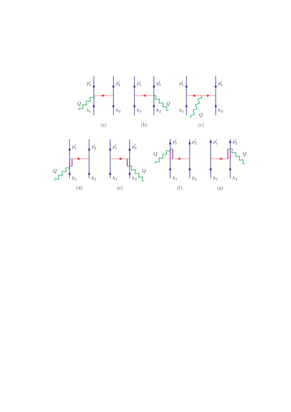
Figure 1: Feynman diagrams for the electromagnetic MEC used in this work.

II.2 2p2h responses and MEC

In this work we apply a fully relativistic model of meson exchange currents (MEC) to compute the electromagnetic response functions in the two-nucleon emission channel (2p-2h). The model was developed for the RFG in Ref. Sim16 .

The 2p-2h hadronic tensor is computed by integrating over all the 2p-2h excitations

$$W^{\mu\nu}_{\rm 2p2h} = \frac{V}{(2\pi)^{9}}\int d^{3}p^{\prime}_{1}d^{3}p^{\prime}_{2}d^{3}h_{1}d^{3}h_{2}\frac{m_{N}^{4}}{E_{1}E_{2}E^{\prime}_{1}E^{\prime}_{2}}w^{\mu\nu}({\bf p}^{\prime}_{1},{\bf p}^{\prime}_{2},{\bf h}_{1},{\bf h}_{2})\;\delta(E^{\prime}_{1}+E^{\prime}_{2}-E_{1}-E_{2}-\omega)$$ (26)

$$\times\Theta(p^{\prime}_{1},h_{1})\Theta(p^{\prime}_{2},h_{2})\delta({\bf p}^{\prime}_{1}+{\bf p}^{\prime}_{2}-{\bf q}-{\bf h}_{1}-{\bf h}_{2})\,,$$

$$\kern-28.45274pt=\frac{V}{(2\pi)^{9}}\int d^{3}p^{\prime}_{1}d^{3}h_{1}d^{3}h_{2}\frac{m_{N}^{4}}{E_{1}E_{2}E^{\prime}_{1}E^{\prime}_{2}}\Theta(p^{\prime}_{1},h_{1})\Theta(p^{\prime}_{2},h_{2})w^{\mu\nu}({\bf p}^{\prime}_{1},{\bf p}^{\prime}_{2},{\bf h}_{1},{\bf h}_{2})\;\delta(E^{\prime}_{1}+E^{\prime}_{2}-E_{1}-E_{2}-\omega)$$

where ${\bf h}_{1}$ and ${\bf h}_{2}$ are the momenta of the holes, with $h_{i}<k_{F}$, while ${\bf p}^{\prime}_{1}$ and ${\bf p}^{\prime}_{2}$ are the momenta of the final particles with $p^{\prime}_{i}>k_{F}$ (Pauli blocking). These two conditions are enforced by the functions $\Theta$ appearing inside the integral, defined as the product of step-functions $\Theta(p^{\prime},h)\equiv\theta(p^{\prime}-k_{F})\theta(k_{F}-h)$.

In Eq. (26) we have integrated over ${\bf p}^{\prime}_{2}$ using the delta-function of momentum conservation with $\bf p^{\prime}_{2}=h_{1}+h_{2}+q-p^{\prime}_{1}$.

The hadronic tensor for a single 2p2h excitation, $w^{\mu\nu}({\bf p}^{\prime}_{1},{\bf p}^{\prime}_{2},{\bf h}_{1},{\bf h}_{2})$, is defined as

$$w^{\mu\nu}({\bf p}^{\prime}_{1},{\bf p}^{\prime}_{2},{\bf h}_{1},{\bf h}_{2})=$$

$$\frac{1}{4}\sum_{s_{1}s_{2}s^{\prime}_{1}s^{\prime}_{2}}\sum_{t_{1}t_{2}t^{\prime}_{1}t^{\prime}_{2}}j^{\mu}(1^{\prime},2^{\prime},1,2)^{*}_{A}j^{\nu}(1^{\prime},2^{\prime},1,2)_{A}$$ (27)

where sums are performed over over spin and isospin third components. Here, the 2p-2h electromagnetic current matrix element is defined as

$$j^{\mu}(1^{\prime},2^{\prime},1,2)\equiv j^{\mu}({\bf p}^{\prime}_{1}s^{\prime}_{1}t^{\prime}_{1},{\bf p}^{\prime}_{2}s^{\prime}_{2}t^{\prime}_{2},{\bf h}_{1}s_{1}t_{1},{\bf h}_{2}s_{2}t_{2})$$ (28)

and the sub-index $A$ means direct minus exchange matrix element

$$j^{\mu}(1^{\prime},2^{\prime},1,2)_{A}\equiv j^{\mu}(1^{\prime},2^{\prime},1,2)-j^{\mu}(1^{\prime},2^{\prime},2,1)\,.$$ (29)

The above integral can be reduced to a 7 dimension integral using the energy conservation function and axial symmetry. Details are given in ref. Sim14 .

The model of relativistic meson-exchange currents correspond to the sum of the Feynman diagrams of Fig. 1 DeP03 ; Sim16 . Diagrams (a,b) represent the seagull (or contact) current, diagram (c) is the pion in flight current, and diagrams (d,e) are the $\Delta$ forward current and (f,g) the $\Delta$ backward current. The total $\Delta(1232)$ excitation current is the sum of forward plus backward diagrams. Specifically the MEC matrix element is written as

$$j^{\mu}(1^{\prime},2,1,2)=j_{\rm sea}^{\mu}+j_{\rm\pi}^{\mu}+j_{\rm\Delta}^{\mu}$$ (30)

The three two-body currents: i) seagull, $j_{\rm sea}^{\mu}$, ii) pion-in-flight, $j_{\rm\pi}^{\mu}$, and iii) $\Delta$ isobar, $j_{\rm\Delta}^{\mu}$, are defined next.

The seagull current matrix element (diagrams (a) and (b) in Fig. 1) is

$$j^{\mu}_{\rm sea}=\frac{f^{2}}{m^{2}_{\pi}}\left[I_{V}^{3}\right]_{1^{\prime}2^{\prime},12}V_{\pi NN}^{s^{\prime}_{1}s_{1}}({\bf p}^{\prime}_{1},{\bf h}_{1})\bar{u}_{s^{\prime}_{2}}({\bf p}^{\prime}_{2})F^{V}_{1}(Q^{2})F_{\pi NN}(k_{1}^{2})\gamma_{5}\gamma^{\mu}u_{s_{2}}({\bf h}_{2})+(1\leftrightarrow 2)\,$$ (31)

where the $\pi NN$ coupling constant is $f=1$, we use the following two-body isospin operator

$$I_{V}^{3} = i\left[\mbox{\boldmath$\tau$}(1)\times\mbox{\boldmath$\tau$}(2)\right]_{z}.$$ (32)

The $\pi NN$ vertex and the pion propagator appear in the spin-dependent function

$$V_{\pi NN}^{s^{\prime}_{1}s_{1}}({\bf p}^{\prime}_{1},{\bf h}_{1})\equiv F_{\pi NN}(k_{1}^{2})\frac{\bar{u}_{s^{\prime}_{1}}({\bf p}^{\prime}_{1})\,\gamma_{5}\not{\!k}_{1}\,u_{s_{1}}({\bf h}_{1})}{k^{2}_{1}-m^{2}_{\pi}},$$ (33)

where $k_{i}^{\mu}=p^{\prime}_{i}{}^{\mu}-h_{i}{}^{\mu}$, $i=1,2$, is the momentum transfer to the $i$th particle, $m_{\pi}$ is the pion mass, and $F_{\pi NN}$ is the strong $\pi NN$ form factor Som78 ; Alb84

$$F_{\pi NN}(k_{1}^{2})=\frac{\Lambda^{2}-m_{\pi}^{2}}{\Lambda^{2}-k_{1}^{2}}$$ (34)

where we use $\Lambda=1300$ MeV. Finally $F_{1}^{V}=F_{1p}-F_{1n}$ is the isovector electromagnetic form factor of the nucleon.

The pion-in-flight or pionic current matrix element follows from diagram (c) in Fig. 1, given as

$$j^{\mu}_{\pi}=\left[I_{V}^{3}\right]_{1^{\prime}2^{\prime},12}\frac{f^{2}}{m^{2}_{\pi}}F^{V}_{1}(Q^{2})V_{\pi NN}^{s^{\prime}_{1}s_{1}}({\bf p}^{\prime}_{1},{\bf h}_{1})V_{\pi NN}^{s^{\prime}_{2}s_{2}}({\bf p}^{\prime}_{2},{\bf h}_{2})\left(k^{\mu}_{1}-k^{\mu}_{2}\right).$$ (35)

Finally, the $\Delta$ current is the sum of forward (diagrams d,e) and backward (f,g) contributions

$$j^{\mu}_{\Delta} = \frac{f^{*}f}{m^{2}_{\pi}}\,V_{\pi NN}^{s^{\prime}_{2}s_{2}}({\bf p}^{\prime}_{2},{\bf h}_{2})\bar{u}_{s^{\prime}_{1}}({\bf p}^{\prime}_{1})F_{\pi N\Delta}(k_{2})\left\{\left[U_{\rm F}^{3}\right]_{1^{\prime}2^{\prime},12}k^{\alpha}_{2}G_{\alpha\beta}(h_{1}+Q)\Gamma^{\beta\mu}(h_{1},Q)\right.$$

$$+\left.\left[U_{\rm B}^{3}\right]_{1^{\prime}2^{\prime},12}\;k^{\beta}_{2}\hat{\Gamma}^{\mu\alpha}(p^{\prime}_{1},Q)G_{\alpha\beta}(p^{\prime}_{1}-Q)\right\}u_{s_{1}}({\bf h}_{1})+(1\leftrightarrow 2).$$

We use the $\pi N\Delta$ coupling constant $f^{*}=2.13$. The forward and backward isospin transition operators are defined by

$$U_{\rm F}^{3} = \sqrt{\frac{3}{2}}\sum_{i}\left(T_{i}T_{3}^{\dagger}\right)\otimes\tau_{i}$$ (36)

$$U_{\rm B}^{3} = \sqrt{\frac{3}{2}}\sum_{i}\left(T_{3}\,T^{\dagger}_{i}\right)\otimes\tau_{i},$$ (37)

where $\vec{T}$ is the transition operator from isospin $\frac{3}{2}$ to $\frac{1}{2}$.

We use the $\pi N\Delta$ strong form factor of Ref. Dek94 , given by

$$F_{\pi N\Delta}(k_{2}^{2})=\frac{\Lambda^{2}_{\Delta}}{\Lambda_{\Delta}^{2}-k_{2}^{2}}$$ (38)

were $\Lambda_{\Delta}=1150$ MeV.

For the electromagnetic $N\rightarrow\Delta$ transition tensor in the forward current, $\Gamma^{\beta\mu}(P,Q)$ we use

$$\Gamma^{\beta\mu}(P,Q)=\frac{C^{V}_{3}}{m_{N}}\left(g^{\beta\mu}\not{\!Q}-Q^{\beta}\gamma^{\mu}\right)\gamma_{5}.$$ (39)

We have kept only the $C_{3}^{V}$ form factor and neglected the smaller contributions of the higher-order terms to the interaction of Ref. Hernandez:2007qq . In the backward current, the vertex tensor is

$$\hat{\Gamma}^{\mu\alpha}(P^{\prime},Q)=\gamma^{0}\left[\Gamma^{\alpha\mu}(P^{\prime},-Q)\right]^{\dagger}\gamma^{0}\,.$$ (40)

Finally, for the $\Delta$-propagator we use

$$G_{\alpha\beta}(P)=\frac{{\cal P}_{\alpha\beta}(P)}{P^{2}-M^{2}_{\Delta}+iM_{\Delta}\Gamma_{\Delta}(P)+\frac{\Gamma_{\Delta}(P)^{2}}{4}}\,.$$ (41)

where ${\cal P}_{\alpha\beta}(P)$ is the spin-$\frac{3}{2}$ projector

$${\cal P}_{\alpha\beta}(P) = -(\not{\!P}+M_{\Delta})\left[g_{\alpha\beta}-\frac{1}{3}\gamma_{\alpha}\gamma_{\beta}-\frac{2}{3}\frac{P_{\alpha}P_{\beta}}{M^{2}_{\Delta}}\right.$$ (42)

$$+ \left.\frac{1}{3}\frac{P_{\alpha}\gamma_{\beta}-P_{\beta}\gamma_{\alpha}}{M_{\Delta}}\right].$$

For the $\Delta$-width, $\Gamma_{\Delta}(P)$ we use the prescription of Dekker Dek94 .

II.3 Inclusion of MEC in the RMF model

In past works Sim16 ; Meg16b ; Sim17 , the 2p2h responses have been computed with the formalism of the previous subsection in the RFG model, including an energy shift $\omega\rightarrow\omega-E_{S}$ to take into account the separation energy of two nucleons $E_{S}\simeq 40$ MeV of finite nuclei that cannot be described in the Fermi gas. This shift is not applied in the electromagnetic form factors of the currents.

In this work we modify the above MEC model for consistency with the relativistic mean field (RMF) of nuclear matter in which the SuSAM^∗ formalism is based. In the RMF the nucleon interacts with the self-consistent mean field in the Hartree approximation (Walecka model), and acquires scalar and vector potential energies. The scalar energy gives rise to the nucleon effective mass

$$m_{N}^{*}=m_{N}-g_{s}\phi_{0}=M^{*}m_{N}$$ (43)

where $g_{s}\phi_{0}$ is the scalar potential energy that depends explicitly on the scalar field $\phi_{0}$ of the RMF Ser86 . On the contrary the vector field, $V_{0}$, of the RMF produces a repulsive potential, $E_{v}=g_{v}V_{0}$, or vector energy, that is added to the on-shell energy to obtain the true nucleon energy

$$E_{true}=E+E_{v}$$ (44)

where $E=\sqrt{p^{2}+(m_{N}^{*})^{2}}$ is the on-shell energy with effective mass $m_{N}^{*}$.

The SuSAM* model is inspired by the 1p-1h quasielastic responses of the RFG, where only differences of energies between initial and final nucleons appear. Therefore the vector energy $E_{v}$ cancels and does not appear in the 1p-1h cross section, and the resulting responses are computed as in the RFG with the change $m_{N}\rightarrow m_{N}^{*}$, except for the electromagnetic current operator Mar17 ; Ama18 . This change has already been specified in the equations of the previous section.

The same cancellation happens in the case of the 2p-2h seagull and pionic current matrix element because the vector energy cancels in the time components of the vectors $k_{1}=p^{\prime}_{1}-h_{1}$ and $k_{2}=p^{\prime}_{2}-h_{2}$. However, in the case of the $\Delta$ current, the $\Delta$ propagator must be computed with the true nucleon energy, including the vector energy. Thus in the forward propagator, $G_{\alpha\beta}(h+Q)$, the hole energy must be the true nucleon energy $h_{0}=E_{h}+E_{v}=(h^{2}+m_{N}^{*2})^{1/2}+E_{v}$. The inclusion of the vector energy affects to the position of the pole in the forward $\Delta$ diagrams, giving rise to the $\Delta$ peak. This allows to determine the value of the vector energy from the experimental data. The same modification must be also applied to the backward propagator $G_{\alpha\beta}(p^{\prime}-Q)$, and to the electromagnetic vertices $\Gamma^{\mu\nu}(h,Q)$ and $\hat{\Gamma}^{\mu\nu}(p^{\prime},Q)$, although in our case these electromagnetic vertices only depend on $Q$.

To finish the implementation of MEC in the RMF we modify the nucleon spinors by using the relativistic effective mass $m^{*}_{N}$ instead of $m_{N}$ in all places except in the form factor $C_{3}^{V}/m_{N}$. All the remaining energies in the hadronic tensor (26) are modified accordingly with the on-shell energy of nucleons with effective mass $m_{N}^{*}$, and the vector energy cancels.

With this procedure we already have at our disposal a consistent model of quasielastic (SuSAM*) plus 2p-2h response functions with relativistic effective mass and vector energy. Note that the use of the effective mass accounts for the nucleon separation energy in both the quasielastic and 2p2h channels.

In the next section we will compare both 2p2h models with and without effective mass, and will use those model to subtract the 2p2h channel to the experimental data of electron scattering.

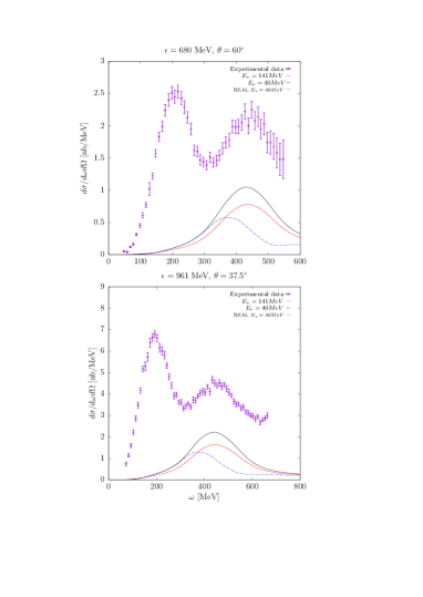
Figure 2: 2p2h contribution to the cross section of ¹²C compared to $(e,e^{\prime})$ data for two experimental kinematics. Black lines are the RFG results with separation energy $E_{s}=40$ MeV, and blue lines are the same model with only the real part of the $\Delta$ propagator. In red are the RMF results with $M^{*}=0.8$ and vector energy $E_{v}=141$ MeV. The experimental data from Ref. archive ; archive2 ; Ben08

III Results

III.1 Obtaining the vector energy

In Fig. 2 we compare the 2p-2h inclusive cross section of the RFG model (with $M^{*}=1$ and separation energy $E_{s}=40$ MeV) to the RMF model (with $M^{*}=0.8$ and $E_{v}=141$ MeV) for electron scattering from ¹²C and two different kinematics. Also shown is the calculation corresponding to the model of ref. Meg16b , where the RFG 2p2h responses were computed using the real part of the denominator of the $\Delta$ propagator, producing smaller cross section peaking at the dip region between the quasielastic and delta peak.

We highlight that in this work we instead use the total delta propagator (real plus imaginary parts) that produces a peak centered in the delta resonance region. This peak describes $\Delta$ excitation decaying inside the nucleus with two nucleon emission instead of pion emission. This decay channel of the $\Delta$ is superposed to the pion emission peak because the same delta propagator contributes to both processes. The differences in the strength of the 2p2h in the two models of fig. 2 with full $\Delta$ propagator (black and red lines) is a result of the relativistic mean field included in the red lines.

The effect of the effective mass is a reduction of the 2p-2h peak and a shift in $\omega$. This shift is not shown in the figure because it cancels out by the vector energy, $E_{v}=141$ MeV, in the $\Delta$ propagator. This value of the vector energy has been fixed such that the $\Delta$ peak in the 2p2h cross section is at the same position as the $\Delta$ resonance of the experimental data.

In fact the maximum of the forward $\Delta$ propagator occurs approximately for $(H+Q)^{2}-M_{\Delta}^{2}=0$. For a nucleon at rest, ${\bf h}=0$, in the RFG, this implies that

$$\omega-E_{S}=\sqrt{M_{\Delta}^{2}+q^{2}}-m_{N}$$ (45)

where $E_{S}\simeq 40$ MeV represents the separation energy of two-nucleon emission that has to be subtracted to the energy transfer. On the other hand, in the RMF model, the condition is

$$\omega=\sqrt{M_{\Delta}^{2}+q^{2}}-m^{*}_{N}-E_{v}$$ (46)

where in this case the separation energy is not needed because it is implicitly included in the scalar potential that gives rise to the relativistic effective mass $m_{N}^{*}=m_{N}-g_{s}\phi_{0}$. Comparing Eqs. (45) and (46) we obtain

$$m_{N}-E_{S}=m_{N}^{*}+E_{v}$$ (47)

from where $E_{v}=m_{N}-m_{N}^{*}-E_{S}\simeq 148$ MeV. This estimated value is in agreement with the fitted value $E_{v}=141$ MeV used in Fig. 2.

The sum of scalar plus vector energy gives the total potential energy of the nucleon

$$U_{0}\equiv-g_{s}\phi_{0}+g_{v}V_{0}=(m^{*}_{N}-m_{N})+E_{v}$$ (48)

In our case, $M^{*}=0.8$, using the fitted value, $E_{v}=141$ MeV, this gives $U_{0}\simeq-47$ MeV for the depth of the nucleon potential energy in ¹²C from our 2p2h model.

This provides a procedure to obtain the vector energy from electron scattering data as a function of the effective mass. We can compare with the values obtained by the model of Serot-Walecka in ref. Ser86 , where $E_{v}=330$ MeV for effective mass $M^{*}=0.6$ in nuclear matter. The corresponding scalar potential is $g_{s}\phi_{0}=376$ MeV. And the depth of the total potential is $U_{0}\simeq-46$ MeV, in good agreement with our findings.

A similar reduction effect of the 2p2h peak due to the relativistic mean field is obtained for the other kinematics. This reduction amounts to $\sim 25\%$ of the RFG model.

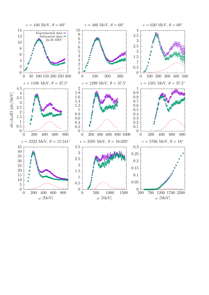
Figure 3: Experimental and subtracted electron scattering data for selected kinematics. The solid lines are the 2p2h cross sections values that are being subtracted, computed with the RMF model with $M^{*}=0.8$. Data from archive ; archive2

III.2 Subtraction of 2p2h cross section from data

Once we have obtained the phenomenological vector energy for our RMF model of 2p2h response, the next step is to subtract the 2p2h contribution from the experimental electron scattering data. The reason is to obtain a better description of the quasielastic scaling function in the SuSAM* model without the 2p2h MEC contamination. Therefore the subtracted data should be a more reliable representation of the 1p1h excitations, and therefore they are more appropriate to be used as a starting point to perform a scaling analysis. Therefore the subtracted data are defined as

$$\left(\frac{d\sigma}{d\Omega^{\prime}d\epsilon^{\prime}}\right)_{sub}\equiv\left(\frac{d\sigma}{d\Omega^{\prime}d\epsilon^{\prime}}\right)_{exp}-\left(\frac{d\sigma}{d\Omega^{\prime}d\epsilon^{\prime}}\right)_{2p2h}$$ (49)

One of the aims of this work is to perform a scaling analysis of the subtracted data, similar to the ones performed in refs. Ama15 ; Ama18 .

First, in Fig. 3 we show the result of the subtraction for some kinematics of ¹²C. The 2p2h curve that is being subtracted from data contributes mainly in the region to the right of the quasielastic peak. Therefore, the subtraction does not modify largely the data around the quasielastic region. The larger effect occurs in the resonance $\Delta$ peak, that is dominated by pion emission. Note that the 2p2h cross section that is being subtracted is not a contribution to pion emission because the final states are two nucleons in the continuum. As we will see below, the contribution of the data in the inelastic region will be irrelevant to the scaling analysis and do not influence the extraction of the quasielastic scaling function.

In Fig. 3 we use the RMF model with $M^{*}=0.8$. We have also made the subtraction with the RFG model (not shown in the figure), where the reduction of the data is larger.

We have performed this subtraction for all the available data of ¹²C. In total there are 2969 entries in the data base. We will use the resulting subtracted data to perform the scaling analysis in the next subsection.

Figure 4: Scaling plot of the subtracted cross section data scaled with the single nucleon function displayed as a function of the scaling variable $\psi^{*}$ using effective mass $M^{*}=0.8$ and Fermi momentum $k_{F}=225$ MeV/c. In the top panel the 2p2h has been computed in the RFG with separation energy $E_{s}=40$ MeV. In the bottom panel the 2p2h are computed in the RMF model with the same value of $M^{*}=0.8$.

III.3 Scaling analysis of subtracted data

We have developed in the past several SuSAM* models obtained by different methods to perform the scaling analysis of $(e,e^{\prime})$ cross section data without the subtraction of the 2p2h. We carried out such analyses in refs. Ama15 ; Ama17 ; Mar17 ; Ama18 . In the SuSAM* models the response functions are computed by using Eq. (7), replacing the RFG scaling function, Eq (8), by a phenomenological function $f^{*}(\psi^{*})$, that is parametrized by Eq. (24). The SuSAM* procedure has proven to be quite robust in the sense that different methods produce similar results for the SuSAM* parameters, verifying self-consistency and superscaling, i.e. that the same scaling function is valid for all the nuclei studied.

In this section from the subtracted experimental data we obtain a new phenomenological scaling function $f^{*}(\psi^{*})$ without the contamination of 2p2h states. One of the goals of this work is to quantify the change of the scaling function due to this subtraction.

To obtain the new scaling function, we first compute for every subtracted datum the experimental value of the scaling function $f^{*}$ by dividing the subtracted cross section by the single nucleon contribution

$$f^{*}=\frac{\left(\frac{d\sigma}{d\Omega^{\prime}d\epsilon^{\prime}}\right)_{\rm sub}}{\sigma_{\rm Mott}\left(v_{L}r_{L}+v_{T}r_{T}\right)}$$ (50)

We also compute the corresponding value of the scaling variable $\psi^{*}$ for that datum. In Fig. 4 we plot $f^{*}$ versus $\psi^{*}$ for all the data of ¹²C. The values of $M^{*}=0.8$ and Fermi momentum $k_{F}=225$ MeV/c have been taken from the previous analyses of refs. Ama15 ; Ama17 ; Mar17 ; Ama18 , where it was shown that these values provide the best scaling of data.

In Fig. 4 we show the subtracted results using the two models of 2p2h discussed above. In the top panel of Fig. 4 the MEC have been computed in the RFG with $M^{*}=1$ and a separation energy. In the bottom panel, the MEC have been computed in the RMF with the same value of the effective mass $M^{*}=0.8$ used to compute the scaling function. In the first case there is an inconsistency because we are using two different values for the nucleon mass: $m_{N}^{*}$ is being used to compute the scaling function and the scaling variable, while $m_{N}$ is being used to compute the MEC 2p2h subtraction. The second case is consistent because we are using always the same value for the nucleon mass, $m_{N}^{*}$. However in both cases the resulting scaling plot is very similar, because both MEC models differ in $\simeq 25$ %.

The most striking thing about the graphs in Fig. 4 is that many points accumulate forming a narrow band or point cloud. This band can be extracted if we eliminate the most scattered data from the plot. To discard the data we apply a density criterion by computing the density of the points in the plot and keeping only those points surrounded by more than 25 points within a circle of radius $r=0.1$. This is the same criterion used in our previous works Ama15 ; Ama17 ; Mar17 ; Ama18 .

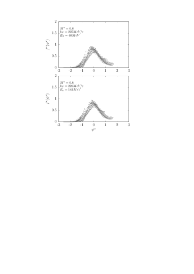
Figure 5: Scaling analysis of the subtracted cross section data after discarding the more scattered data by a density criterion. The selected data are shown for the two models of the 2p2h cross section of Fig. 4.

In Fig. 5 we show the selected data resulting from the application of the density criterion. All the inelastic data points go away and only the points around the QE region survive as a thick band. In past works we obtained the QE bands without subtraction of the 2p2h cross section. In the present work the 2p2h contribution is not present in the data points. Besides, we observe that both bands are very similar in both MEC models. In the top case (RFG) a total of 1546 data points from the total 2969 points survive. In the bottom case (RMF) the band contains 1453 data points. However, both bands are almost identical. Note that the selected points accumulate around the values of the scaling function of the RMF (for nuclear matter) $f_{RMF}=3(1-\psi^{*2})\theta(1-\psi^{*2})/4$. However the cloud of data points extend outside the interval $-1<\psi^{*}<1$, where the RMF scaling function is zero. Specifically, most of the data points are in the range $-1.5<\psi^{*}<1.5$.

Note that the density criterion is one choice to approximate the region where more data collapse, and where a band is clearly visible with defined edges. This choice provides an estimate of the degree of scaling violation, from the width of the resulting band, because it is clear that the data do not scale exactly, but only approximately.

		$a_{1}$	$a_{2}$	$a_{3}$	$b_{1}$	$b_{2}$	$b_{3}$
	central	-0.0465	0.469	0.633	0.707	1.073	0.202
Old band	min	-0.0270	0.442	0.598	0.967	0.705	0.149
	max	-0.0779	0.561	0.760	0.965	1.279	0.200
	central	-0.0971	0.422	0.477	0.299	0.855	0.330
New band	min	-0.0419	0.437	0.575	0.759	0.625	0.152
	max	-0.1594	0.585	0.759	0.863	0.965	0.230

Table 1: Parameters of the central value of the phenomenological scaling function, $f^{*}(\psi^{*})$, and those of the lower and upper boundaries (min and max, respectively) of the bands.

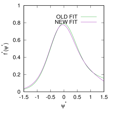
Figure 6: Comparison between the phenomenological scaling function obtained in this work with 2p2h subtraction (new fit) and the scaling function obtained in ref. Ama17 without subtraction (old fit).

The phenomenological scaling function in the subtracted SuSAM^∗ model is defined by a fit to the selected data points, with a function that we parameterize as a combination of two Gaussian functions, Eq. (24). This provides the central value of the band. This scaling function gives the best approximation to the quasi-elastic data in the SuSAM* model. The resulting new scaling function is shown in Fig. 6, where it is compared with the old scaling function obtained without subtracting the 2p-2h Ama17 . The parameters of the new and old fits are given in Table 1.

Concerning the theoretical error coming from scaling violation in the quasielastic data of Fig. 5, we estimate it by fitting the maximum and minimum values in the point cloud. This is done by choosing an enough small bin size in $\psi^{*}$ in order to determine a subset of points defining the experimental borders of the band. We divide the interval of the variable $\psi^{*}$ into sub-intervals of width $\epsilon$ (bins). Within each bin of $\psi^{*}$ we calculate the maximum and minimum of the scaling function of all the points within the bin. These maximums and minimums define the points of the upper and lower edges. These edges are fitted separately as sums of two gaussians similarly to Eq. (24). The resulting theoretical band is shown in Fig. 7, where it is compared to the band fitted without subtraction of 2p2h Ama17 . The central scaling function previously fitted provides the best approximation to the selected data points, and therefore to the quasielastic cross section without 2p2h, within a theoretical error given by the band.

Note that the bands of Fig. 7, fitted with and without 2p2h contribution, are very similar. The small differences are due to the slight change of some data after subtraction, but the quasielastic region defined by them is unaltered by MEC. This is because the data that are most affected by MEC are those that are later removed by the selection process. These results confirm that the SuSAM* approach to select the QE data is consistent with or without the subtraction. What we have achieved with subtraction is a better definition of the tail to the right of the scaling function, which extends above $\psi^{*}=1.5$.

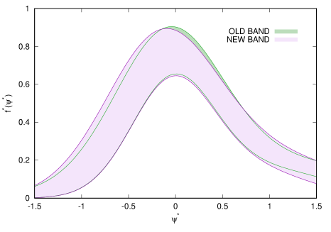
Figure 7: The quasielastic band of the scaling function obtained in the present work with subtraction of 2p2h cross section, compared to the old band fitted in ref. Ama17 without subtraction.

III.4 Cross section results

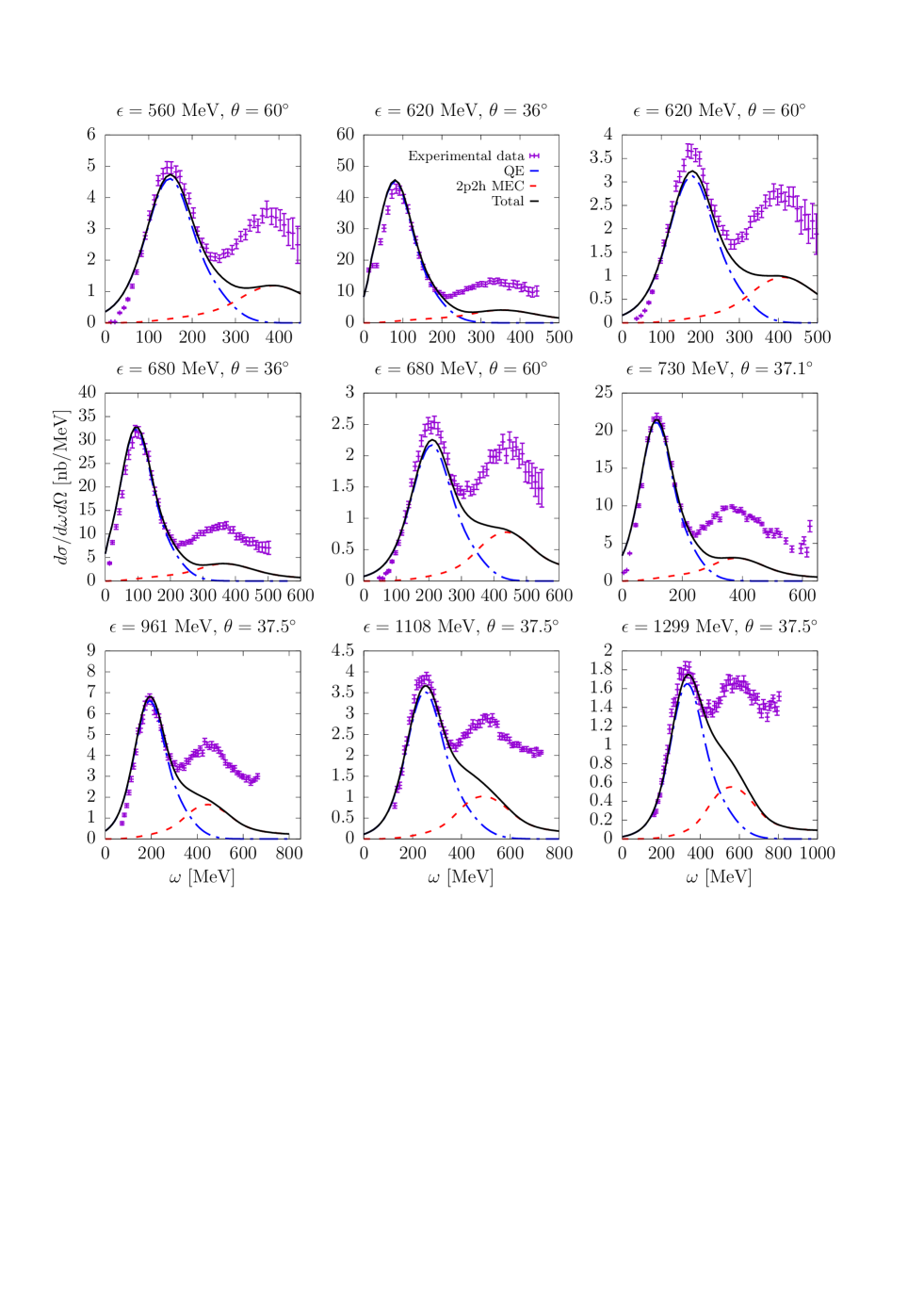
Figure 8: Inclusive electron scattering cross section of ¹²C for selected kinematics. Results are shown for the new SuSAM* model, with the phenomenological scaling function fitted in this work, for the 2p2h contribution in the RMF model, and the total SuSAM*+MEC*. The experimental data data are from ref. Ben08 ; archive ; archive2

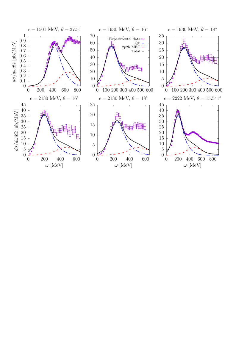
Figure 9: The same as Fig. 8 for other kinematics. Data are from ref. Ben08 ; archive ; archive2

In this section we use the phenomenological scaling function obtained in the previous section to compute the $(e,e^{\prime})$ cross section, and evaluate the effect of adding the 2p2h cross section computed in the RMF. Since the phenomenological scaling function does not contain contamination from 2p2h emission, it is safe to add the 2p2h directly to the SuSAM* model, obtaining a consistent 1p1h+2p2h model with relativistic effective mass (SuSAM*+MEC*). Pion emission in not included in the present model.

Our cross section results are compared to experimental data of ¹²C$(e,e^{\prime})$ for selected kinematics in Figs. 8 and 9. In the last panel of Fig. 9 we also compare with the new data for ¹²C performed in a recent experiment at JLab Dai18 . In general, the region of quasielastic peak is well reproduced by the model. The MEC contribute mainly in the region to the right of the maximum QE peak (dip region) and go into the pion emission region, where the maximum of the 2p-2h is reached, contributing to the resonant $\Delta$ peak. The total SuSAM*+MEC* results should be complemented with a pion emission model in order to reproduce the total cross section in this region.

IV Conclusions

In this work we have extended the superscaling analysis with relativistic effective mass to include the effects of meson-exchange currents. The SuSAM* approach takes into account the effects of the relativistic mean field inside the nucleus, that induces an effective mass and vector energy to the nucleons. The effects of 2p2h MEC are first subtracted from the data before performing the scaling analysis, and later they are added to the SuSAM* cross section to obtain the total SuSAM*+MEC* (2p2h) cross section. The MEC matrix elements are computed in nuclear matter by modifying the nucleon spinors and the energies according to the solutions of the mean-field relativistic equation with scalar and vector potentials in the Walecka model Ser86 . Thus, the 2p2h contribution is computed using the same ingredients as the SuSAM* 1p1h model, namely the same value for the relativistic effective mass $m_{N}^{*}$.

A novelty in this work is that the MEC depend on the nucleon vector energy. That energy does not appear in the 1p1h responses due to the cancellation between final and initial nucleons. Using our MEC model we have been able to estimate the value of the vector energy from the $(e,e^{\prime})$ data for ¹²C, $E_{v}\simeq 141$ MeV, and $M^{*}=0.8$, in accord with Serot and Walecka Ser86 .

We have verified that the new scaling function $f^{*}(\psi^{*})$ obtained from the scaling analysis of the ¹²C subtracted data —experimental minus theoretical 2p2h cross section— is very similar to the one obtained in a previous work without subtraction of the MEC contribution. This is because that scaling analysis is based in a robust data selection method, by elimination of the data that do not collapse into the quasielastic point cloud. Therefore, in this work we have shown the strength of the SuSAM* selection method.

Finally, we have computed the total cross section of 1p1h plus 2p2h and compared to data. The MEC contribution modifies the cross section to the right of the quasielastic peak, reaching the $\Delta$ peak, where the pion emission and inelastic contribution (not included in this work) are more important.

In future work we will extend this MEC model to the weak sector to compute the effect of 2p2h in charge-changing neutrino scattering, that was analyzed with the SuSAM* model, without including MEC, in Ref. Rui18 .

V Acknowledgments

This work has been partially supported by the Spanish Ministerio de Economia y Competitividad (grants No. FIS2017-85053-C2-1-P) and by the Junta de Andalucia (grant No. FQM-225). V.L.M.C. acknowledges a contract funded by Agencia Estatal de Investigacion and Fondo Social Europeo.

References

- (1) J. E. Amaro, M. B. Barbaro, J. A. Caballero, R. González-Jiménez, G. D. Megias and I. Ruiz Simo, J. Phys. G 47 (2020) no.12, 124001
- (2) U. Mosel, Ann. Rev. Nuc. Part. Sci. 66 (2016), 171.
- (3) T. Katori and M. Martini, J. Phys. G 45 (2018) no.1, 013001.
- (4) L. Alvarez-Ruso, Y. Hayato, J. Nieves, New J. Phys. 16 (2014) 075015.
- (5) A. M. Ankowski, C. Mariani, J. Phys. G44 (2017) 054001.
- (6) O. Benhar, P. Huber, C. Mariani, D. Meloni, Phys. Rep. 700 (2017) 1.
- (7) V Lyubushkin et al. (NOMAD Collaboration), Eur. Phys. J. C 63 (2009), 355.
- (8) A. Aguilar-Arevalo et al. (MiniBooNE Collaboration), Phys. Rev. D 81, 092005 (2010).
- (9) A. Aguilar-Arevalo et al. (MiniBooNE Collaboration), Phys. Rev. D 88, 032001 (2013).
- (10) G.A. Fiorentini et al. (MINERvA Collaboration) Phys. Rev. Lett. 111, 022502 (2013).
- (11) K. Abe et al., (T2K Collaboration), Phys. Rev. D 87, 092003 (2013).
- (12) K. Abe et al., (T2K Collaboration), Phys. Rev. D93 (2016) 112012.
- (13) K. Abe et al. (T2K Collaboration), Phys. Rev. D 97 (2018), 012001.
- (14) M. Martini, M. Ericson, G. Chanfray, J. Marteau, Phys.Rev. C80 (2009) 065501.
- (15) J. Nieves, I. Ruiz Simo, M.J. Vicente Vacas, Phys.Rev. C83 (2011) 045501.
- (16) K. Gallmeister, U. Mosel and J. Weil, Phys. Rev. C 94, no. 3, 035502 (2016).
- (17) G. D. Megias, M. V. Ivanov, R. Gonzalez-Jimenez, M. B. Barbaro, J. A. Caballero, T. W. Donnelly and J. M. Udias, Phys. Rev. D 89, no. 9, 093002 (2014) Erratum: [Phys. Rev. D 91, no. 3, 039903 (2015)]
- (18) A. M. Ankowski, Phys. Rev. D 92, no. 1, 013007 (2015).
- (19) R. Gran, J. Nieves, F. Sanchez and M. J. Vicente Vacas, Phys. Rev. D 88, no. 11, 113007 (2013).
- (20) V. Pandey, N. Jachowicz, M. Martini, R. Gonzalez-Jimenez, J. Ryckebusch, T. Van Cuyck and N. Van Dessel, Phys. Rev. C 94, no. 5, 054609 (2016)
- (21) M. Martini, N. Jachowicz, M. Ericson, V. Pandey, T. Van Cuyck and N. Van Dessel, Phys. Rev. C 94, no. 1, 015501 (2016).
- (22) G. D. Megias, J. E. Amaro, M. B. Barbaro, J. A. Caballero and T. W. Donnelly, Phys. Rev. D 94, 013012 (2016).
- (23) G.D Megias, J. E. Amaro, M. B. Barbaro, J. A. Caballero, T. W. Donnelly and I. Ruiz Simo, Phys. Rev. D 94 (2016), 093004.
- (24) A. Lovato, S. Gandolfi, J. Carlson, Steven C. Pieper, R. Schiavilla, Phys.Rev.Lett. 117 (2016) 082501.
- (25) V. Pandey, N. Jachowicz, T. Van Cuyck, J. Ryckebusch and M. Martini, Phys. Rev. C 92, no. 2, 024606 (2015).
- (26) A. M. Ankowski, O. Benhar, M. Sakuda, Phys. Rev. D 91, 033005 (2015).
- (27) N. Rocco, A. Lovato, O. Benhar, Phys.Rev.Lett. 116 (2016) 192501.
- (28) J. E. Amaro, M. B. Barbaro, J. A. Caballero, T. W. Donnelly and A. Molinari, Phys. Rept. 368, 317 (2002).
- (29) J. E. Amaro, M. B. Barbaro, J. A. Caballero, T. W. Donnelly and C. Maieron, Phys. Rev. C 71, 065501 (2005).
- (30) J. A. Caballero, J. E. Amaro, M. B. Barbaro, T. W. Donnelly and J. M. Udias, Phys. Lett. B 653, 366 (2007).
- (31) J. M. Udias, J. A. Caballero, E. Moya de Guerra, J. E. Amaro and T. W. Donnelly, Phys. Rev. Lett. 83, 5451 (1999).
- (32) A. Bodek, M.E. Christy, and B. Coopersmith, Eur. Phys. Jou. C 74, 3091 (2014).
- (33) A. Gil, J. Nieves and E. Oset, Nucl. Phys. A 627 (1997) 543.
- (34) I. Ruiz Simo, J. E. Amaro, M. B. Barbaro, A. De Pace, J. A. Caballero and T. W. Donnelly, J.Phys. G44 (2017) no.6, 065105.
- (35) J. Nieves, J.E. Sobczyk, Annals Phys. 383 (2017) 455.
- (36) W.M. Alberico, A. Molinari, T.W. Donnelly, E. L. Kronenberg, and J.W. Van Orden, Phys Rev. C 38 (1988) 1801.
- (37) T. W. Donnelly and I. Sick, Phys. Rev. Lett. 82, 3212 (1999).
- (38) T. W. Donnelly and I. Sick, Phys. Rev. C 60, 065502 (1999).
- (39) C. Maieron, T. W. Donnelly and I. Sick, Phys. Rev. C 65, 025502 (2002).
- (40) J. E. Amaro, M. B. Barbaro, J. A. Caballero, T. W. Donnelly, A. Molinari, I. Sick, Phys. Rev. C 71, 015501 (2005).
- (41) C.J. Horowitz, D.P. Murdock, and B.D. Serot, in Computational Nuclear Physics Vol. 1, Springer-Verlag, Berlin 1991.
- (42) R. Gonzalez-Jimenez, G.D. Megias, M.B. Barbaro, J.A. Caballero, and T.W. Donnelly, Phys. Rev. C 90, 035501 (2014).
- (43) J. E. Amaro, E. Ruiz Arriola and I. Ruiz Simo, Phys. Rev. C 92, no. 5, 054607 (2015).
- (44) J. E. Amaro and E. Ruiz Arriola, I. Ruiz Simo, Phys. Rev. D 95, 076009 (2017).
- (45) V. L. Martinez-Consentino, I. Ruiz Simo, J. E. Amaro and E. Ruiz Arriola, Phys. Rev. C 96, no. 6, 064612 (2017).
- (46) J. E. Amaro, V. L. Martinez-Consentino, E. Ruiz Arriola and I. Ruiz Simo, Phys. Rev. C 98 (2018) 024627
- (47) I. Ruiz Simo, V. L. Martinez-Consentino, J. E. Amaro and E. Ruiz Arriola, Phys. Rev. D 97, 116006 (2018).
- (48) R. Rosenfelder, Ann. Phys. (N.Y.) 128, 188 (1980).
- (49) B.D. Serot, and J.D. Walecka, Adv. Nucl. Phys. 16 (1986) 1.
- (50) K. Wehrberger, Phys. Rep. 225 (1993) 273.
- (51) O. Benhar, D. Day and I. Sick, arXiv:nucl-ex/0603032.
- (52) O. Benhar, D. Day, and I. Sick, http://faculty.virginia.edu/qes-archive/
- (53) O. Benhar, D. Day, and I. Sick, Rev Mod Phys. 80 (2008) 189.
- (54) H. Dai et al., (JLab Hall A Collaboration), arXiv:1803.01910 [nucl-ex].
- (55) M.B. Barbaro, R. Cenni, A. De Pace, T.W. Donnelly, A. Molinari, Nucl. Phys. A 643 (1998) 137.
- (56) T. De Forest, Nucl. Phys. A 392, 232 (1983).
- (57) S. Galster, H. Klein, J. Moritz, K. H. Schmidt, D. Wegener and J. Bleckwenn, Nucl. Phys. B 32, 221 (1971).
- (58) I. Ruiz Simo, C. Albertus, J. E. Amaro, M. B. Barbaro, J. A. Caballero and T. W. Donnelly, Phys. Rev. D 90 (2014) no.3, 033012
- (59) A. De Pace, M. Nardi, W. M. Alberico, T. W. Donnelly and A. Molinari, Nucl. Phys. A 726 (2003), 303-326
- (60) B. Sommer, Nucl. Phys A 308 (1978) 263.
- (61) W. Alberico, M. Ericson, and A. Molinari, Ann. Phys. (N.Y.) 154 (1984) 356.
- (62) M. J. Dekker, P. J. Brussaard, and J. A. Tjon Phys. Rev. C 49 (1994) 2650
- (63) E. Hernandez, J. Nieves and M. Valverde, Phys. Rev. D 76 (2007) 033005.
- (64) I. Ruiz Simo, J. E. Amaro, M. B. Barbaro, J. A. Caballero, G. D. Megias and T. W. Donnelly, Phys. Lett. B 770, 193-199 (2017)