Modelling sub-daily precipitation extremes with the blended generalised extreme value distribution

Abstract

A new method is proposed for modelling the yearly maxima of sub-daily precipitation, with the aim of producing spatial maps of return level estimates. Yearly precipitation maxima are modelled using a Bayesian hierarchical model with a latent Gaussian field, with the blended generalised extreme value (bGEV) distribution used as a substitute for the more standard generalised extreme value (GEV) distribution. Inference is made less wasteful with a novel two-step procedure that performs separate modelling of the scale parameter of the bGEV distribution using peaks over threshold data. Fast inference is performed using integrated nested Laplace approximations (INLA) together with the stochastic partial differential equation (SPDE) approach, both implemented in R-INLA. Heuristics for improving the numerical stability of R-INLA with the GEV and bGEV distributions are also presented. The model is fitted to yearly maxima of sub-daily precipitation from the south of Norway, and is able to quickly produce high-resolution return level maps with uncertainty. The proposed two-step procedure provides an improved model fit over standard inference techniques when modelling the yearly maxima of sub-daily precipitation with the bGEV distribution.

¹ Norwegian University of Science and Technology (NTNU)
² University of Glasgow
³ King Abdullah University of Science and Technology (KAUST)

Keywords: bGEV distribution, Block maxima modelling, INLA, Spatial statistics

1 Introduction

Heavy rainfall over short periods of time can cause flash floods, large economic losses and immense damage to infrastructure. The World Economic Forum states that climate action failure and extreme weather events are perceived among the most likely and most impactful global risks in 2021 [64]. Therefore, a better understanding of heavy rainfall can be of utmost importance for many decision-makers, e.g., those that are planning the construction or maintenance of important infrastructure. In this paper, we create spatial maps with estimates of large return levels for sub-daily precipitation in Norway. Estimation of return levels is best described within the framework of extreme value theory, where the most common methods are the block maxima and the peaks over threshold [16, 12, e.g.]. Due to low data quality (see Section 2 for more details) and the difficulty of selecting high-dimensional thresholds, we choose to use the block maxima method for estimating the precipitation return levels. This method is based on modelling the maximum of a large block of random variables with the generalised extreme value (GEV) distribution, which is the only non-degenerate limit distribution for a standardised block maximum [21]. When working with environmental data, blocks are typically chosen to have a size of one year [12]. Inference with the GEV distribution is difficult, partially because its support depends on its parameter values. [11] propose to ease inference by substituting the GEV distribution with the blended generalised extreme value (bGEV) distribution, which has the right tail of a Fréchet distribution and the left tail of a Gumbel distribution, resulting in a heavy-tailed distribution with a parameter-free support. Both [11] and [60] demonstrate with simulation studies that the bGEV distribution performs well as a substitute for the GEV distribution when estimating properties of the right tail. Additionally, in this paper we develop a simulation study that shows how the parameter-dependent support of the GEV distribution can lead to numerical problems during inference, while inference with the bGEV distribution is more robust. This can be of crucial importance in complex and high-dimensional settings, and consequently we choose to model the yearly maxima of sub-daily precipitation using the bGEV distribution.

Modelling of extreme daily precipitation has been given much attention in the literature, and it is well established that precipitation is a heavy-tailed phenomenon [63, 32, 47, e.g.], which makes the bGEV distribution a possible model for yearly precipitation maxima. Spatial modelling of extreme daily precipitation has also received a great amount of interest. [13] combine Bayesian hierarchical modelling with a generalised Pareto likelihood for estimating large return values for daily precipitation. Similar methods are also applied by [52, 25, 17, 46], using either the block maxima or the peaks over threshold approach. Using a multivariate peaks over threshold approach, [9] propose local likelihood inference for a specific factor copula model to deal with complex non-stationary dependence structures of precipitation over the contiguous U.S. Spatial modelling of extreme sub-daily precipitation is more difficult, due to less available data sources. Consequently, this is often performed using intensity-duration-frequency relationships where one pools together information from multiple aggregation times in order to estimate return levels [35, 58, 36, 61]. Spatial modelling of extreme hourly precipitation in Norway has previously been performed by [19]. After their work was published, the number of observational sites for hourly precipitation in Norway has greatly increased. We aim to improve their return level estimates by including all the new data that have emerged over the last years. We model sub-daily precipitation using a spatial Bayesian hierarchical model with a bGEV likelihood and a latent Gaussian field. In order to keep our model simple, we do not pool together information from multiple aggregation times, making our model purely spatial. The model assumes conditional independence between observations, which makes it able to estimate the marginal distribution of extreme sub-daily precipitation at any location, but unable to successfully estimate joint distributions over multiple locations. In the case of hydrological processes such as precipitation, ignoring dependence might lead to an underestimation of the risk of flooding. However, [17] find that models where the response variables are independent given some latent process can be a good choice when the aim is to estimate a spatial map of marginal return levels.

High-resolution spatial modelling can demand a lot of computational resources and be highly time-consuming. The framework of integrated nested Laplace approximations [49, INLA;] allows for a considerable speed-up by using numerical approximations instead of sampling-based inference methods like Markov chain Monte Carlo (MCMC). Inference with a spatial Gaussian latent field can be even further sped up with the so-called stochastic partial differential equation [39, SPDE;] approach of representing a Gaussian random field using a Gaussian Markov random field that is the approximate solution of a specific SPDE. Both INLA and the SPDE approach have been implemented in the R-INLA library, which is used for performing inference with our model [3, 50, 1]. R-INLA requires a log-concave likelihood to ensure numerical stability during inference. However, neither the GEV likelihood nor the bGEV likelihood are log-concave, which can cause inferential issues. We present heuristics for mitigating the risk of numerical instability caused by a lack of log-concavity.

A downside of the block maxima method is that inference can be somewhat wasteful compared to the peaks over threshold method. Additionally, most of the available weather stations in Norway that measure hourly precipitation are young and contain quite short time series. This data sparsity makes it challenging to place complex models on the parameters of the bGEV distribution in the hierarchical model. A promising method of accounting for data-sparsity is the recently developed sliding block estimator, which allows for better data utilisation by not requiring that the block maxima used for inference come from disjoint blocks [6, 65]. However, to the best of our knowledge, no theory has yet been developed for using the disjoint block estimator on non-stationary time series, or for performing Bayesian inference with the disjoint block estimator. [60] propose a new two-step procedure that allows for less wasteful and more stable inference with the block maxima method by separately modelling the scale parameter of the bGEV distribution using peaks over threshold data. Having modelled the scale parameter, one can standardise the block maxima so the scale parameter can be considered as a constant, and then estimate the remaining bGEV parameters. [7] suggests that, when modelling stationary time series, the peaks over threshold technique is preferable over block maxima if the interest lies in estimating large quantiles of the stationary distribution of the times series. The opposite holds if the interest lies in estimating return levels, i.e. quantiles of the distribution of the block maxima. Thus, both methods have different strengths, and by using this two-step procedure, one can take advantage of the merits and improve the pitfalls of both methods. We apply the two-step procedure for modelling sub-daily precipitation and compare the performance with that of a standard block maxima model where all the bGEV parameters are estimated jointly.

The remainder of the paper is organised as follows. Section 2 introduces the hourly precipitation data and all explanatory variables used for modelling. Section 3 presents the bGEV distribution and describes the Bayesian hierarchical model along with the two-step modelling procedure. Additionally, heuristics for improving the numerical stability of R-INLA are proposed, and a score function for evaluating model performance is presented. In Section 4 we perform modelling of the yearly precipitation maxima in Norway. A cross-validation study is performed for evaluating the model fit, and a map of return levels is estimated. Conclusions are presented in Section 5.

2 Data

2.1 Hourly precipitation data

Observations of hourly aggregated precipitation from a total of 380 weather stations in the south of Norway are downloaded from an open archive of historical weather data from MET Norway (https://frost.met.no). The oldest weather stations contain observations from 1967, but approximately 90 percent of the available weather stations are established after 2000. Each observation comes with a quality code, but almost all observations from before 2005 are of unknown quality. An inspection of the time series with unknown quality detects unrealistic precipitation observation ranging from $-300$ mm/hour to $400$ mm/hour. Other unrealistic patterns, like $50$ mm/hour precipitation for more than three hours in a row, or no precipitation during more than half a year, are also detected. The data set contains large amounts of missing data, but these are often recorded as 0 mm/hour, instead of being recorded as missing. Thus, there is no way of knowing which of the zeros represent missing data and which represent an hour without precipitation. Having detected all of this, we decide to remove all observations with unknown or bad quality flags, which accounts for approximately $14\%$ of the total number of observations. Additionally, we clean the data by removing all observations from years with more than $30\%$ missing data and from years where more than two months contain less than $20\%$ of the possible observations. This data cleaning is performed to increase the probability that our observed yearly maxima are close or equal to the true yearly maxima. Having cleaned the data, we are left with $72\%$ of the original observations, distributed over 341 weather stations and spanning the years 2000 to 2020. The total number of usable yearly maxima is approximately 1900. Figure 1 displays the distribution of the number of usable yearly precipitation maxima per weather station. The majority of the weather stations contain five or less usable yearly maxima, and approximately 50 stations have more than 10 usable maxima. Figure 1 also displays the location of all the weather stations. A large amount of the stations are located close to each other, in the southeast of Norway. Such spatial clustering can be an indicator for preferential sampling. However, we do not believe that preferential sampling is an issue for our data. The weather stations are mostly placed in locations with high population densities, and to the best of our knowledge there is no strong dependency between population density and extreme precipitation in Norway, as there are large cities located both in dry and wet areas of the country. Even though most stations are located in areas with high population densities, there is still a good spatial coverage of the entire area of interest, also for areas with low population densities.

The yearly maxima of precipitation accumulated over $1,2,\ldots,24$ hours are computed for all locations and available years. A rolling window approach with a step size of 1 hour is used for locating the precipitation maxima. As noted by [48], a sampling frequency of one hour is not enough to observe the exact yearly maximum of hourly precipitation. With this sampling frequency, one only observes the precipitation during the periods 00:00-01:00, 01:00-02:00, etc., whereas the maximum precipitation might occur e.g. during the period 14:23-15:23. Approximately half of the available weather stations have a sampling frequency of one minute, while the other half only contain hourly observations. We therefore use a sampling frequency of one hour for all weather stations, as this allows us to use all the 341 weather stations without having to account for varying degrees of sampling frequency bias in our model.

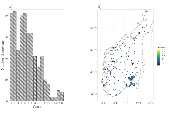
Figure 1: a) A histogram displaying the number of usable yearly precipitation maxima for all the weather stations used in this paper. b) The location of the 341 weather stations. The number of usable yearly precipitation maxima from each station are displayed using different colours. Note that some points overlap in areas with high station densities.

[19] used the same data source for estimating return levels of hourly precipitation. They fitted their models to hourly precipitation maxima using only 69 weather stations from all over Norway. However, they received a cleaned data set from the Norwegian Meteorological Institute, resulting in time series with lengths up to 45 years. Our data cleaning approach is more strict than that of [19] in the sense that it results in shorter time series by removing all data of uncertain quality. On the other hand, we include more locations and get a considerably better spatial coverage, by keeping all time series with at least one good year of observations.

The main focus of this paper is the novel methodology for fast and accurate estimation of return levels, and we believe that we have prepared the data well enough to give a good demonstration of our proposed model and to achieve reliable return level estimates for sub-daily precipitation. It is trivial to add more, or differently cleaned data, to improve the return level estimates at a later time.

2.2 Explanatory variables

We use one climate-based and four orographic explanatory variables. These are displayed in Table 1. Altitude is extracted from a digital elevation model of resolution $50\times 50$ m², from the Norwegian Mapping Authority (https://hoydedata.no). The distance to the open sea is computed using the digital elevation model. Precipitation climatologies for the period 1981-2010 are modelled by [14]. The climatologies do not cover the years 2011-2020, from which most of the observations come. We assume that the precipitation patterns have not changed overly much and that they are still representative for the years 2011-2020. [30] find that, in most southern regions of Norway, the only season with a significant increase in precipitation is Autumn. This strengthens our assumption that the change in precipitation patterns is slow enough to not be problematic for us.

[19] include additional explanatory variables in their model, such as temperature, summer precipitation and the yearly number of wet days. They find mean summer precipitation to be one of the most important explanatory variables. We compute these explanatory variables at all station locations using the gridded seNorge2 data product [40, 41]. Our examination finds that yearly precipitation, summer precipitation and the yearly number of wet days are close to $90\%$ correlated with each other. There is also a negative correlation between temperature and altitude of around -$85\%$. Consequently, we choose to not use any more explanatory variables for modelling, as highly correlated variables might lead to identifiability issues during parameter estimation.

Table 1: Explanatory variables used for modelling sub-daily precipitation extremes. The two rightmost columns show which explanatory variables are used for modelling which parameters of the bGEV distribution for yearly precipitation (see Section 3.2).

Explanatory variable	Description	Unit	$\textbf{x}_{\mu}$	$\textbf{x}_{\sigma}$
Mean annual precipitation	Mean annual precipitation for the years 1981-2010	mm	✓
Easting	Eastern coordinate (UTM 32)	km	✓	✓
Northing	Northern coordinate (UTM 32)	km	✓	✓
Altitude	Height above sea level	m	✓
Distance to the open sea	Shortest distance to the open sea	km	✓	✓

3 Methods

3.1 The bGEV distribution

Extreme value theory concerns the statistical behaviour of extreme events, possibly larger than anything ever observed. It provides a framework where probabilities associated with these events can be estimated by extrapolating into the tail of the distribution. This can be used for e.g. estimating large quantiles, which is the aim of this work [16, 12, e.g.]. A common approach in extreme value theory is the block maxima method. Assume that the limiting distribution of the standardised block maximum $(Y_{k}-b_{k})/a_{k}$ is non-degenerate, where $Y_{k}=\max\{X_{1},X_{2},\ldots,X_{k}\}$ is the maximum over $k$ random variables from a stationary stochastic process, and $\{b_{k}\}$ and $\{a_{k}>0\}$ are some appropriate sequences of standardising constants. Then, for large enough block sizes $k$, the distribution of the block maximum $Y_{k}$ is approximately equal to the GEV distribution with [21, 12]

$$P(Y_{k}\leq y)\approx\begin{cases}\exp\left\{-[1+\xi(y-\mu_{k})/\sigma_{k}]^{-1/\xi}_{+}\right\},&\xi\neq 0,\\ \exp\left\{-\exp[-(y-\mu_{k})/\sigma_{k}]\right\},&\xi=0,\end{cases},$$ (1)

where $(a)_{+}=\max\{a,0\}$, $\sigma_{k}>0$ and $\mu_{k},\xi\in\mathbb{R}$. In most settings, $k$ is fixed, so we denote $\sigma=\sigma_{k}$ and $\mu=\mu_{k}$. A challenge with the GEV distribution is that its support depends on its parameters. This complicates inference procedures such as maximum likelihood estimation [5, 54, e.g.], and can be particularly problematic in a covariate-dependent setting with spatially varying parameters, as it might also introduce artificial boundary restrictions such as an unnaturally large lower bound for yearly maximum precipitation. [11] propose the bGEV distribution as an alternative to the GEV distribution in settings where the tail parameter $\xi$ is non-negative. The support of the bGEV distribution is parameter-free and infinite. This allows for more numerically stable inference, while also avoiding the possibility of estimated lower bounds that are larger than future observations. The bGEV distribution function is

$$H(y;\mu,\sigma,\xi,a,b)={F(y;\mu,\sigma,\xi)}^{v(y;a,b)}{G(y;\tilde{\mu},\tilde{\sigma})}^{1-v(y;a,b)},$$ (2)

where $F$ is a GEV distribution with $\xi\geq 0$ and $G$ is a Gumbel distribution. The weight function is equal to

$$v(y;a,b)=F_{\beta}\left(\frac{y-a}{b-a};c_{1},c_{2}\right),$$

where $F_{\beta}(\cdot;c_{1},c_{2})$ is the distribution function of a beta distribution with parameters $c_{1}=c_{2}=5$, which leads to a symmetric and computationally efficient weight function. The weight $v(y;a,b)$ is zero for $y\leq a$ and one for $y\geq b$, meaning that the left tail of the bGEV distribution is equal to the left tail in $G$, while the right tail is equal to the right tail in $F$. The choice of the weight $v(y;a,b)$ should not considerably affect inference if we let the difference between $a$ and $b$ be small. The parameters $\tilde{\mu}$ and $\tilde{\sigma}$ are injective functions of $(\mu,\sigma,\xi)$ such that the bGEV distribution function is continuous and $F(y;\mu,\sigma,\xi)=G(y;\tilde{\mu},\tilde{\sigma})$ for $y\in\{a,b\}$. Setting $a=F^{-1}(p_{a})$ and $b=F^{-1}(p_{b})$ with small probabilities $p_{a}=0.1,\ p_{b}=0.2$ makes it possible to model the right tail of the GEV distribution without any of the problems caused by a finite left tail. See [11] for guidelines on how to choose $c_{1}$, $c_{2}$, $p_{a}$ and $p_{b}$.

In the supplementary material we present a simulation study where both the GEV distribution and the bGEV distribution are fitted to univariate samples from a GEV distribution. We demonstrate how a small change in initial values can cause large numerical problems for inference with the GEV distribution, and no noticeable difference for inference with the bGEV distribution. The fact that considerable numerical problems can arise for the GEV distribution in a univariate setting with large sample sizes and perfectly GEV-distributed data strongly indicates that the GEV distribution is not robust enough to be used reliably in complex, high-dimensional problems with noisy data. The bGEV distribution is more robust than the GEV distribution, and we therefore prefer it over the GEV distribution for modelling precipitation maxima in Norway.

Although the bGEV distribution is more robust than the GEV distribution, it might still seem unnatural to model block maxima using the bGEV distribution, when it is known that the correct limiting distribution is the GEV distribution. However, we argue that the bGEV would be a good choice for modelling heavy tailed block maxima even if it had not been more robust than the GEV distribution. In multivariate extreme value theory it is common to assume that the tail parameter $\xi$ of the GEV distribution is constant in time and/or space [46, 35, 10, 51, e.g.]. This assumption is often made, not because one truly believes that it should be constant, but because estimation of $\xi$ is difficult, and models with a constant $\xi$ often are “good enough”. The tail parameter is incredibly important for the shape of the GEV distribution, and small changes in $\xi$ can lead to large changes in return levels, and even affects the existence of distributional moments. A model where $\xi$ varies in space can therefore e.g. provide model fits with a finite mean in one location and an infinite mean in the neighbouring location. Such a model can also give scenarios where a new observation at one location can change the existence of moments in other, possibly far away, locations. Thus, even though it might seem unnatural to use a constant tail parameter, these models often provide more natural fits to data than the models that allow $\xi$ to vary in space. We claim that the bGEV distribution fulfils a similar role as a model with constant $\xi$, but for the model support instead of the moments. When $\xi$ is positive, the support of the GEV distribution varies with its parameter values. In regression settings with covariates and finite amounts of data one can therefore experience unnatural lower bounds that are known to be wrong. Furthermore, if only one new observation is smaller than the estimated lower limit, the entire model fit will be invalidated. We therefore prefer the bGEV, which completely removes the lower bound while still having the right tail of the GEV distribution, thus yielding a model that is “good enough” for estimating return levels, but without the unwanted model properties in the left tail of the GEV distribution.

Naturally, the bGEV distribution can only be applied for modelling exponential- or heavy-tailed phenomena $(\xi\geq 0)$. However, it is well established that extreme precipitation should be modelled with a non-negative tail parameter. [13] performs Bayesian spatial modelling of extreme daily precipitation in Colorado and find that the tail parameter is positive and less than 0.15. [47] examine more than 15000 records of daily precipitation worldwide and conclude that the Fréchet distribution performs the best. They propose that even when the data suggests a negative tail parameter, it is more reasonable to use a Gumbel or Fréchet distribution. Less information is available concerning the distribution of extreme sub-daily precipitation. However, [35] argues that the distribution of precipitation should not have an upper bound for any aggregation period, so $\xi$ must be non-negative. [59] estimate the distribution of yearly precipitation maxima in Belgium for aggregation times down to 1 minute, and find that the estimates of $\xi$ increase as the aggregation times decreases, meaning that the tail parameter for sub-daily precipitation should be larger than for daily precipitation. [20] estimate $\xi$ for daily precipitation in Norway from the seNorge1 data product [57, 44] and conclude that the tail parameter estimates are non-constant in space and often negative. However, the authors do not provide confidence intervals or p-values and do not state whether the estimates are significantly different from zero. Based on our own exploratory analysis (results not shown) and the overwhelming evidence in the literature, we assume that sub-daily precipitation is a heavy-tailed phenomenon.

Following [11], we reparametrise the bGEV distribution from $(\mu,\sigma,\xi)$ to $(\mu_{\alpha},\sigma_{\beta},\xi)$, where the location parameter $\mu_{\alpha}$ is equal to the $\alpha$ quantile of the bGEV distribution if $\alpha\geq p_{b}$. The scale parameter $\sigma_{\beta}$, hereby denoted the spread parameter, is equal to the difference between the $1-\beta/2$ quantile and the $\beta/2$ quantile of the bGEV distribution if $\beta/2\geq p_{b}$. There is a one to one relationship between the new and the old parameters. The new parametrisation is advantageous as it is considerably easier to interpret than the old parametrisation. The parameters $\mu_{\alpha}$ and $\sigma_{\beta}$ are directly connected to the quantiles of the bGEV distribution, whereas $\mu$ and $\sigma$ have no simple connections with any kind of moments or quantiles. Consequently, it is much easier to choose informative priors for $\mu_{\alpha}$ and $\sigma_{\beta}$. Based on preliminary experiments, we find that $\alpha=0.5$ and $\beta=0.8$ are good choices that makes it easy to select informative priors. This is because the empirical quantiles close to the median have less variance. We have also experienced that R-INLA is more numerically stable when the spread is small, i.e. $\beta$ is large.

3.2 Models

Let $y_{t}(\bm{s})$ denote the maximum precipitation at location $\bm{s}\in\mathcal{S}$ during year $t\in\mathcal{T}$, where $\mathcal{S}$ is the study area and $\mathcal{T}$ is the time period in focus. We assume a bGEV distribution for the yearly precipitation maxima,

$$\left[y_{t}(\bm{s})|\mu_{\alpha}(\bm{s}),\sigma_{\beta}(\bm{s}),\xi(\bm{s})\right]\sim\text{bGEV}(\mu_{\alpha}(\bm{s}),\sigma_{\beta}(\bm{s}),\xi(\bm{s})),$$

where all observations are assumed to be conditionally independent given the parameters $\mu_{\alpha}(\bm{s})$, $\sigma_{\beta}(\bm{s})$ and $\xi(\bm{s})$. Correct estimation of the tail parameter is a difficult problem which highly affects estimates of large quantiles. The tail parameter is assumed to be constant, i.e. $\xi(\bm{s})=\xi$. As discussed in Section 3.1, this is a common procedure, as inference for $\xi$ is difficult with little data. The tail parameter is further restricted such that $\xi<0.5$, resulting in a finite mean and variance for the yearly maxima. This restriction makes inference easier and more numerically stable. Exploratory analysis of our data supports the hypothesis of a spatially constant $\xi<0.5$ and spatially varying $\mu_{\alpha}(\bm{s})$ and $\sigma_{\beta}(\bm{s})$ (results not shown). Two competing models are constructed for describing the spatial structure of $\mu_{\alpha}(\bm{s})$ and $\sigma_{\beta}(\bm{s})$.

3.2.1 The joint model

In the first model, denoted the joint model, both parameters are modelled using linear combinations of explanatory variables. Additionally, to draw strength from neighbouring stations, a spatial Gaussian random field is added to the location parameter. This gives the model

$$\left[y_{t}(\bm{s})|\mu_{\alpha}(\bm{s}),\sigma_{\beta}(\bm{s}),\xi\right] \sim\text{bGEV}(\mu_{\alpha}(\bm{s}),\sigma_{\beta}(\bm{s}),\xi),$$ (3)

$$\mu_{\alpha}(\bm{s}) =\textbf{x}_{\mu}(\bm{s})^{T}\bm{\beta}_{\mu}+u_{\mu}(\bm{s}),$$

$$\log\left(\sigma_{\beta}(\bm{s})\right) =\textbf{x}_{\sigma}(\bm{s})^{T}\bm{\beta}_{\sigma},$$

where $\textbf{x}_{\mu}(\bm{s})$ and $\textbf{x}_{\sigma}(\bm{s})$ are vectors containing an intercept plus the explanatory variables described in Table 1, and $\bm{\beta}_{\mu}$ and $\bm{\beta}_{\sigma}$ are vectors of regression coefficients. The term $u_{\mu}(\bm{s})$ is a zero-mean Gaussian field with Matérn correlation function, i.e.,

$$\text{Corr}(u_{\mu}(\bm{s}_{i}),u_{\mu}(\bm{s}_{j}))=\frac{1}{2^{\nu-1}\Gamma(\nu)}\left(\sqrt{8\nu}\frac{d(\bm{s}_{i},\bm{s}_{j})}{\rho}\right)^{\nu}K_{\nu}\left(\sqrt{8\nu}\frac{d(\bm{s}_{i},\bm{s}_{j})}{\rho}\right).$$

Here, $d(\bm{s}_{i},\bm{s}_{j})$ is the Euclidean distance between $\bm{s}_{i}$ and $\bm{s}_{j}$, $\rho>0$ is the range parameter and $\nu>0$ is the smoothness parameter. The function $K_{\nu}$ is the modified Bessel function of the second kind and order $\nu$. The Matérn family is a widely used class of covariance functions in spatial statistics due to its flexible local behaviour and attractive theoretical properties [55, 42, 28]. Its form also naturally appears as the covariance function of some models for the spatial structure of point rain rates [56]. Efficient inference for high-dimensional Gaussian random fields can be achieved using the SPDE approach of [39], which is implemented in R-INLA. It is common to fix the smoothness parameter $\nu$ instead of estimating it, as the parameter is difficult to identify from data. The SPDE approximation in R-INLA allows for $0<\nu\leq 1$. We choose $\nu=1$ as this reflects our beliefs about the smoothness of the underlying physical process. Additionally, [62] argues that $\nu=1$ is a more natural choice for spatial models than the less smooth exponential correlation function $(\nu=1/2)$, and $\nu=1$ is also the most extensively tested value when using R-INLA with the SPDE approach [38].

The joint model is similar to the models of [25, 19, 17]. However, they all place a Gaussian random field in the linear predictor for the log-scale and for the tail parameter. Within the R-INLA framework, it is not possible to model the spread or the tail using Gaussian random fields. Based on the amount of available data and the difficulty of estimating the spread and tail parameters, we also believe that the addition of a spatial Gaussian field in either parameter would simply complicate parameter estimation without any considerable contributions to model performance. Consequently, we do not include any Gaussian random field in the spread or tail of the bGEV distribution.

3.2.2 The two-step model

The second model is specifically tailored for sparse data with large block sizes. In such data-sparse situations, a large observation at a single location can be explained by a large tail parameter or a large spread parameter. In practice this might cause identifiability issues between $\sigma_{\beta}(\bm{s})$ and $\xi$, even though the parameters are identifiable in theory. In order to put a flexible model on the spread while avoiding such issues, [60] propose a model which borrows strength from the peaks over threshold method for separate modelling of $\sigma_{\beta}(\bm{s})$.

For some large enough threshold $x_{thr}(\bm{s})$, the distribution of sub-daily precipitation $X(\bm{s})$ larger than $x_{thr}(\bm{s})$ is assumed to follow a generalised Pareto distribution [18]

$$P(X(\bm{s})>x_{thr}(\bm{s})+x|X(\bm{s})>x_{thr}(\bm{s}))=\left(1+\frac{\xi x}{\zeta(\bm{s})}\right)^{-1/\xi},$$

with tail parameter $\xi$ and scale parameter $\zeta(\bm{s})=\sigma(\bm{s})+\xi(x_{thr}(\bm{s})-\mu(\bm{s}))$, where $\mu(\bm{s})$ and $\sigma(\bm{s})$ are the original GEV parameters from (1). Since $\xi$ is assumed to be constant in space, all spatial variations in the bGEV distribution must stem from $\mu(\bm{s})$ or $\sigma(\bm{s})$. We therefore assume that the difference $x_{thr}(\bm{s})-\mu(\bm{s})$ between the threshold and the location parameter is proportional to the scale parameter $\sigma(\bm{s})$. This assumption leads to the spread $\sigma_{\beta}(\bm{s})$ being proportional to the standard deviation of all observations larger than the threshold $x_{thr}(\bm{s})$. Based on this assumption, it is possible to model the spatial structure of the spread parameter independently of the location and tail parameter. Denote

$$\sigma_{\beta}(\bm{s})=\sigma_{\beta}^{*}\cdot\sigma^{*}(\bm{s}),$$

with $\sigma_{\beta}^{*}$ a standardising constant and $\sigma^{*}(\bm{s})$ the standard deviation of all observations larger than $x_{thr}(\bm{s})$ at location $\bm{s}$. Conditional on $\sigma^{*}(\bm{s})$, the block maxima can be standardised as

$$y_{t}^{*}(\bm{s})=y_{t}(\bm{s})/\sigma^{*}(\bm{s}).$$

The standardised block maxima have a bGEV distribution with a constant spread parameter,

$$\left[y^{*}_{t}(\bm{s})|\mu_{\alpha}^{*}(\bm{s}),\sigma_{\beta}^{*},\xi\right]\sim\text{bGEV}(\mu_{\alpha}^{*}(\bm{s}),\sigma_{\beta}^{*},\xi),$$

where $\mu_{\alpha}^{*}(\bm{s})=\mu_{\alpha}(\bm{s})/\sigma^{*}(\bm{s})$. Consequently, the second model is divided into two steps. First, we model the standard deviation of large observations at all locations. Second, we standardise the block maxima observations and model the remaining parameters of the bGEV distribution. We denote this as the two-step model. The two-step model shares some similarities with regional frequency analysis [15, 31, 45, 8], which is a multi-step procedure where the data are standardised and pooled together inside homogeneous regions. However, we standardise the data differently and do not pool together data from different locations. Instead, we borrow strength from nearby locations by adding a spatial Gaussian random fields to our model and by keeping $\xi$ constant for all locations.

The location parameter $\mu^{*}_{\alpha}(\bm{s})$ is modelled as a linear combination of explanatory variables $\textbf{x}_{\mu}(\bm{s})$ and a Gaussian random field $u_{\mu}(\bm{s})$, just as $\mu_{\alpha}(\bm{s})$ in the joint model (3). For estimation of $\sigma^{*}(\bm{s})$, the threshold $x_{thr}(\bm{s})$ is chosen as the $99\%$ quantile of all observed precipitation at location $\bm{s}$. The precipitation observations larger than $x_{thr}(\bm{s})$ are declustered to account for temporal dependence, and only the cluster maximum of an exceedance is used for estimating $\sigma^{*}(\bm{s})$. This might sound counter-intuitive, as the aim of the two-step model is to use more data to simplify inference. However, even when only using the cluster maxima, inference is less wasteful than for the joint model. By using all threshold exceedances for estimating $\sigma^{*}(\bm{s})$, we would need to account for the dependence within exceedance clusters, which would add another layer of complexity to the modelling procedure. Consequently, we have chosen to not model the temporal dependence and only use the cluster-maxima for inference in this paper. To avoid high uncertainty from locations with few observations, $\sigma^{*}(\bm{s})$ is only computed at stations with more than three years of data. In order to estimate $\sigma^{*}(\bm{s})$ at locations with little or no observations, a linear regression model is used, where the logarithm of $\sigma^{*}(\bm{s})$ is assumed to have a Gaussian distribution,

$$\left[\log\left(\sigma^{*}(\bm{s})\right)|\eta(\bm{s}),\tau\right]\sim\mathcal{N}(\eta(\bm{s}),\tau^{-1}),$$

with precision $\tau$ and mean $\eta(\bm{s})=\textbf{x}_{\sigma}(\bm{s})^{T}\bm{\beta}_{\sigma}$. The estimated posterior mean from the regression model is then used as an estimator for $\sigma^{*}(\bm{s})$ at all locations. Consequently, the complete two-step model is given as

$$\left[\log\left(\sigma^{*}(\bm{s})\right)|\eta(\bm{s}),\tau\right] \sim\mathcal{N}(\eta(\bm{s}),\tau^{-1}),$$ (4)

$$\eta(\bm{s}) =\textbf{x}_{\sigma}(\bm{s})^{T}\bm{\beta}_{\sigma},$$

$$\left[y^{*}_{t}(\bm{s})|\mu_{\alpha}^{*}(\bm{s}),\sigma_{\beta}^{*},\xi\right] \sim\text{bGEV}(\mu_{\alpha}^{*}(\bm{s}),\sigma_{\beta}^{*},\xi),$$

$$y^{*}_{t}(\bm{s}) =y_{t}(\bm{s})/\sigma^{*}(\bm{s}),$$

$$\mu_{\alpha}^{*}(\bm{s}) =\textbf{x}_{\mu}(\bm{s})^{T}\bm{\beta}_{\mu}+u_{\mu}(\bm{s}).$$

Notice that the formulation of the two-step model makes it trivial to add more complex components for modelling the spread. One can, therefore, easily add a spatial Gaussian random field to the linear predictor of $\log(\sigma^{*}(\bm{s}))$ while still using the R-INLA framework for inference, which is not possible with the joint model. In Section 4 we perform modelling both with and without a Gaussian random field in the spread to test how it affects model performance.

The uncertainty in the estimator for $\sigma^{*}(\bm{s})$ is not propagated into the bGEV model for the standardised response, meaning that the estimated uncertainties from the two-step model are likely to be too small. This can be corrected with a bootstrapping procedure, where we draw $B$ samples from the posterior of $\log(\sigma^{*}(\bm{s}))$ and estimate $(\mu^{*}_{\alpha}(\bm{s}),\sigma^{*}_{\beta},\xi)$ for each of the $B$ samples. [60] show that the two-step model with 100 bootstrap samples is able to outperform the joint model in a simple setting.

It might seem contradictory to employ a model based on exceedances in our setting, since we claim that the data quality is too bad to use the peaks over threshold model for estimating return levels. However, merely estimating the standard deviation of all threshold exceedances is a much simpler task than to estimate spatially varying parameters of the generalised Pareto distribution, including the tail parameter $\xi$. Thus, while we claim that the available data is not of good enough quality to estimate return levels in a similar fashion to [46], we also claim that it is of good enough quality to perform the simple task of estimating the trends in the spread parameter. The estimation of all remaining parameters, including $\xi$, is performed using block maxima data, which we believe to be of better quality.

3.3 INLA

By placing a Gaussian prior on $\bm{\beta}_{\mu}$, both the joint and the two-step models fall into the class of latent Gaussian models. This is advantageous as it allows for inference using INLA with the R-INLA library [49, 50, 3]. The extreme value framework is quite new to the R-INLA package. Still, in recent years, some papers have started to appear where it is used for modelling extremes with INLA [46, 10, e.g.]. R-INLA includes an implementation of the SPDE approximation for Gaussian random fields with a Matérn correlation function, which is used on the random field $u_{\mu}(\bm{s})$ for a considerable improvement in inference speed.

A requirement for using INLA is that the model likelihood is log-concave. Unfortunately, neither the GEV distribution nor the bGEV distribution have log-concave likelihoods when $\xi>0$. This can cause severe problems for model inference. However, we find that these problems are mitigated by choosing slightly informative priors for the model parameters, which is possible because of the reparametrisation described in Section 3.1. Additionally, we find that R-INLA is more stable when given a response that is standardised such that the difference between its $95\%$ quantile and its $5\%$ quantile is equal to 1. Based on the authors’ experience, similar standardisation of the response is also a common procedure when using INLA for estimating the Weibull distribution parameters within the field of survival analysis. We believe that the combination of slightly informative priors and standardisation of the response is enough to fix the problems of non-concavity and ensure that R-INLA is working well with the bGEV distribution.

3.4 Evaluation

Model performance can be evaluated using the continuous ranked probability score [43, 26, 22, CRPS;],

$$\text{CRPS}(F,y)=\int_{-\infty}^{\infty}(F(t)-I(t\geq y))^{2}\text{d}t=2\int_{0}^{1}\ell_{p}\left(y-F^{-1}(p)\right)\text{d}p,$$ (5)

where $F$ is the forecast distribution, $y$ is an observation, $\ell_{p}(x)=x(p-I(x<0))$ is the quantile loss function and $I(\cdot)$ is an indicator function. The CRPS is a strictly proper scoring rule, meaning that the expected value of $\text{CRPS}(F,y)$ is minimised for $G=F$ if and only if $y\sim G$. The importance of proper scoring rules when forecasting extremes is discussed by [37]. From (5), one can see that the CRPS is equal to the integral over the quantile loss function for all possible quantiles. However, we are only interested in predicting large quantiles, and the model performance for small quantiles is of little importance to us. The threshold weighted CRPS [27, twCRPS;] is a modification of the CRPS that allows for emphasis on specific areas of the forecast distribution,

$$\text{twCRPS}(F,y)=2\int_{0}^{1}\ell_{p}\left(y-F^{-1}(p)\right)w(p)\text{d}p,$$ (6)

where $w(p)$ is a non-negative weight function. A possible choice of $w(p)$ for focusing on the right tail is the indicator function $w(p)=I(p>p_{0})$. As described by [4], the mean twCRPS is not robust to outliers and it gives more weight to forecast distributions with large variances, i.e. at locations far away from any weather station. A scaled version of the twCRPS, denoted the StwCRPS, is created using theorem 5 of [4]:

$$S_{\text{scaled}}(F,y)=\frac{S(F,y)}{|S(F,F)|}+\log\left(|S(F,F)|\right),$$ (7)

where $S(F,y)$ is the twCRPS and $S(F,F)$ is its expected value with respect to the forecast distribution,

$$S(F,F)=\int S(F,y)\text{d}F(y).$$

The mean StwCRPS is more robust to outliers and varying degrees of uncertainty in forecast distributions, while still being a proper scoring rule [4].

Using R-INLA we are able to sample from the posterior distribution of the bGEV parameters at any location $\bm{s}$. The forecast distribution at location $\bm{s}$ is therefore given as

$$\widehat{F}_{\bm{s}}(\cdot)=\frac{1}{m}\sum_{i=1}^{m}F(\cdot;\mu_{\alpha}^{(i)}(\bm{s}),\sigma_{\beta}^{(i)}(\bm{s}),\xi^{(i)}),$$ (8)

where $F$ is the distribution function of the bGEV distribution and $(\mu_{\alpha}^{(i)}(\bm{s}),\sigma_{\beta}^{(i)}(\bm{s}),\xi^{(i)})$ are drawn from the posterior distribution of the bGEV parameters for $i=1,\ldots,m$, where $m$ is a multiple of the number $B$ of bootstrap samples. A closed-form expression is not available for the twCRPS when using the forecast distribution from (8). Consequently, we evaluate the twCRPS and StwCRPS using numerical integration.

4 Modelling sub-daily precipitation extremes in Norway

The models from Section 3 are applied for estimating return levels in the south of Norway. Table 1 shows which explanatory variables are used for modelling the location and spread parameters in both models. All explanatory variables are standardised to have zero mean and a standard deviation of 1, before being applied for modelling. Inference for the two-step model is performed both with and without propagation of the uncertainty in $\sigma^{*}(\bm{s})$. The uncertainty propagation is achieved using 100 bootstrap samples, as described in Section 3.2.2. Additionally, we modify the two-step model and add a random Gaussian field $u_{\sigma}(\bm{s})$ to the linear predictor of the log-spread, to test if this can yield any considerable improvement in model performance. Just as $u_{\mu}(\bm{s})$, $u_{\sigma}(\bm{s})$ has zero mean and a Matérn covariance function.

4.1 Prior selection

Priors must be specified before we can model the precipitation extremes. From construction, the location parameter $\mu_{\alpha}$ is equal to the $\alpha$ quantile of the bGEV distribution. This allows us to place a slightly informative prior on $\bm{\beta}_{\mu}$, using quantile regression on $y^{*}(\bm{s})$ [33, 34]. We choose a Gaussian prior for $\bm{\beta}_{\mu}$, centred at the $\alpha$ quantile regression estimates and with a precision of 10. There is no unit on the precision in $\bm{\beta}_{\mu}$ because the block maxima have been standardised, as described in Section 3.3. The regression coefficients $\bm{\beta}_{\sigma}$ differ between the two-step and joint models. In the joint model, all the coefficients in $\bm{\beta}_{\sigma}$, minus the intercept coefficient, are given Gaussian priors with zero mean and a precision of $10^{-3}$. The intercept coefficient, here denoted $\beta_{0,\sigma}$, is given a log-gamma prior with parameters such that $\exp(\beta_{0,\sigma})$ has a gamma prior with mean equal to the empirical difference between the $1-\beta/2$ quantile and the $\beta/2$ quantile of the standardised block maxima. The precision of the gamma prior is 10. In the two-step model, all coefficients of $\bm{\beta}_{\sigma}$ are given Gaussian priors with zero mean and a precision of $10^{-3}$, while the logarithm of $\sigma_{\beta}^{*}$ is given the same log-gamma prior as the intercept coefficient in the joint model.

The parameters of the Gaussian random fields $u_{\mu}$ and $u_{\sigma}$ are given penalised complexity (PC) priors. The PC prior is a weakly informative prior distribution, designed to punish model complexity by placing an exponential prior on the distance from some base model [53]. [23] develop a joint PC prior for the range $\rho>0$ and standard deviation $\zeta>0$ of a Gaussian random field, where the base model is defined to have infinite range and zero variance. The prior contains two penalty parameters, that can be decided by specifying the four parameters $\rho_{0}$, $\alpha_{1}$, $\zeta_{0}$ and $\alpha_{2}$ such that $P(\rho<\rho_{0})=\alpha_{1}$ and $P(\zeta>\zeta_{0})=\alpha_{2}$. We choose $\alpha_{1}=\alpha_{2}=0.05$. $\rho_{0}$ is given a value of 75 km for both the random fields, meaning that we place a $95\%$ probability on the range being larger than 75 km. To put this range into context, the study area has a dimension of approximately $730\times 460$ km², and the mean distance from one station to its closest neighbour is 10 km. $\zeta_{0}$ is given a value of $0.5$ mm for $u_{\sigma}$, meaning that we place a $95\%$ probability on the standard deviation being smaller than $0.5$ mm. This seems to be a reasonable value because the estimated logarithm of $\sigma^{*}(\bm{s})$ lies in the range between $0.1$ mm and $3.5$ mm for all available weather stations and all examined aggregation times. For $u_{\mu}$ we set $\zeta_{0}=0.5$, which is a reasonable value because of the standardisation of the response described in Section 3.3.

A PC prior is also placed on the tail parameter $\xi$. [46] develop a PC prior for the tail parameter of the generalised Pareto distribution, which is the default prior for $\xi$ in R-INLA when modelling with the bGEV distribution. However, to the best of our knowledge, expressions for the PC priors for $\xi$ in the GEV or bGEV distributions are not previously available in the literature. In the supplementary material we develop expressions for the PC prior of $\xi\in[0,1)$ with base model $\xi=0$ for the GEV distribution and the bGEV distribution. Closed-form expressions do not exist, but the priors can be approximated numerically. Having computed the PC priors for the GEV distribution and the bGEV distribution, we find that they are similar to the PC prior of the generalised Pareto distribution, which has a closed-form expression and is already implemented in R-INLA. Consequently, we choose to model the tail parameter of the bGEV distribution with the PC prior for the generalised Pareto distribution [46]:

$$\pi(\xi)=\frac{\lambda}{\sqrt{2}}\exp\left(-\frac{\lambda}{\sqrt{2}}\frac{\xi}{(1-\xi)^{1/2}}\right)\left(\frac{1-\xi/2}{(1-\xi)^{3/2}}\right),$$

with $0\leq\xi<1$ and penalty parameter $\lambda$. Even though the prior is defined for values of $\xi$ up to 1, a reparametrisation is performed within R-INLA such that $0\leq\xi<0.5$. Since the base model has $\xi=0$, the prior places more weight on small values of $\xi$ when $\lambda$ increases. Based on the plots in Figure S2.1 in the supplementary material, we find a value of $\lambda=7$ to give a good description of our prior beliefs, as we expect $\xi$ to be positive but small.

4.2 Cross-validation

Model performance is evaluated using five-fold cross-validation with the StwCRPS. The StwCRPS weight function is chosen as $w(p)=I(p>0.9)$. Both in-sample and out-of-sample performance are evaluated. The mean StwCRPS over all five folds are displayed in Table 2. The two-step model outperforms the joint model for all aggregation times. This implies that information about threshold exceedances can provide valuable information when modelling block maxima. When performing in-sample estimation, the variant of the two-step model with a Gaussian field and without bootstrapping always outperforms the other contestants. However, during out-of-sample estimation, the model performs worse than its competitors. This indicates a tendency to overfit when not using bootstrapping to propagate uncertainty in $\sigma^{*}(\bm{s})$ into the estimation of $(\mu_{\alpha}^{*}(\bm{s}),\sigma^{*}_{\beta},\xi)$. The two variants of the two-step model that use bootstrapping perform best during out-of-sample estimation. While their model fits yield similar scores, their difference in complexity is quite considerable, as one model contains two spatial random fields, and the other only contains one. This shows that there is little need for placing an overly complex model on the spread parameter. Consequently, for estimation of the bGEV parameters and return levels, we choose to use the two-step model with bootstrapping and without a spatial Gaussian random field in the spread.

Table 2: Mean StwCRPS with weight function $w(p)=I(p>0.9)$ for 5-fold cross-validation performed using out-of-sample estimation and in-sample estimation. The two-step method is tested with and without a Gaussian field in the spread and bootstrapping for propagation of uncertainty. Cross-validation is performed for precipitation aggregated over periods of 1 hour, 3 hours, 6 hours, 12 hours and 24 hours. The best scores are written in bold.

	Model	$u_{\sigma}(\bm{s})$	Boot-	1 h	3 h	6 h	12 h	24 h
			strap
Out-of-	Joint			$-0.872$	$-0.597$	$-0.412$	$-0.149$	$0.0500$
sample	Two-step	✓	✓	$\bm{-0.905}$	$\bm{-0.603}$	$-0.427$	$-0.207$	$\bm{0.0425}$
	Two-step	✓		$-0.893$	$-0.585$	$-0.414$	$-0.197$	$0.0635$
	Two-step		✓	$-0.876$	$-0.594$	$\bm{-0.429}$	$\bm{-0.211}$	$0.0456$
	Two-step			$-0.872$	$-0.584$	$-0.417$	$-0.196$	$0.0674$
In-	Joint			$-0.876$	$-0.608$	$-0.445$	$-0.230$	$0.0206$
sample	Two-step	✓	✓	$-1.004$	$-0.713$	$-0.564$	$-0.328$	$-0.1066$
	Two-step	✓		$\bm{-1.012}$	$\bm{-0.721}$	$\bm{-0.577}$	$\bm{-0.333}$	$\bm{-0.1161}$
	Two-step		✓	$-0.889$	$-0.607$	$-0.453$	$-0.247$	$-0.0244$
	Two-step			$-0.886$	$-0.607$	$-0.454$	$-0.243$	$-0.0182$

4.3 Parameter estimates

The parameters of the two-step model are estimated for different aggregation times between 1 and 24 hours. Uncertainty is propagated using $B=100$ bootstrap samples. Estimation of the posterior of $(\mu_{\alpha}^{*}(\bm{s}),\sigma^{*}_{\beta},\xi)$ given some value of $\sigma^{*}(\bm{s})$ takes less than 2 minutes on a 2.4 gHz laptop with 16 GB RAM, and the 100 bootstraps can be computed in parallel. On a moderately sized computational server, inference can thus be performed in well under 10 minutes.

The estimated values of the regression coefficients $\bm{\beta}_{\mu}$ and $\bm{\beta}_{\sigma}$, the spread $\sigma_{\beta}^{*}$ and the standard deviation of the Gaussian field $u_{\mu}(\bm{s})$ for the standardised precipitation maxima, are displayed in Table 3 for some selected temporal aggregations. These estimates are computed by drawing 20 samples from each of the $100$ posterior distributions. The empirical mean, standard deviation and quantiles of these 2000 samples are then reported.

Table 3: Estimated regression coefficients $\bm{\beta}_{\mu}$, $\bm{\beta}_{\sigma}$ and estimated standard deviation $\text{SD}(u_{\mu})$ of the Gaussian field $u_{\mu}(\bm{s})$ in the two-step model for yearly maximum precipitation at different temporal aggregations.

Temporal	Parameter	Explanatory	Mean	SD	$2.5\%$	$50\%$	$97.5\%$
aggregation		variable			quantile	quantile	quantile
1 hour	$\bm{\beta}_{\mu}$	Intercept	$0.669$	$0.066$	$0.518$	$0.675$	$0.794$
		Mean annual precipitation	$0.071$	$0.012$	$0.044$	$0.072$	$0.091$
		Altitude	$-0.006$	$0.011$	$-0.026$	$-0.006$	$0.013$
		Easting	$-0.044$	$0.035$	$-0.118$	$-0.042$	$0.017$
		Northing	$0.036$	$0.038$	$-0.036$	$0.036$	$0.111$
		Distance to the open sea	$-0.001$	$0.033$	$-0.072$	$0.002$	$0.055$
	$\text{SD}(u_{\mu})$		$0.084$	$0.023$	$0.047$	$0.085$	$0.127$
	$\sigma^{*}_{\beta}$		$0.118$	$0.002$	$0.113$	$0.118$	$0.123$
	$\bm{\beta}_{\sigma}$	Intercept	$2.836$	$0.007$	$2.822$	$2.831$	$2.835$
		Easting	$0.088$	$0.015$	$0.058$	$0.078$	$0.087$
		Northing	$-0.150$	$0.015$	$-0.177$	$-0.160$	$-0.151$
		Distance to the open sea	$-0.050$	$0.017$	$-0.080$	$-0.062$	$-0.051$
3 hours	$\bm{\beta}_{\mu}$	Intercept	$0.847$	$0.025$	$0.800$	$0.846$	$0.895$
		Mean annual precipitation	$0.120$	$0.012$	$0.096$	$0.122$	$0.139$
		Altitude	$-0.009$	$0.009$	$-0.027$	$-0.010$	$0.007$
		Easting	$0.016$	$0.021$	$-0.025$	$0.017$	$0.057$
		Northing	$0.022$	$0.018$	$-0.015$	$0.024$	$0.054$
		Distance to the open sea	$0.017$	$0.018$	$-0.021$	$0.017$	$0.052$
	$\text{SD}(u_{\mu})$		$0.062$	$0.013$	$0.045$	$0.060$	$0.085$
	$\sigma^{*}_{\beta}$		$0.123$	$0.003$	$0.117$	$0.123$	$0.129$
	$\bm{\beta}_{\sigma}$	Intercept	$3.207$	$0.017$	$3.177$	$3.190$	$3.208$
		Easting	$0.031$	$0.014$	$0.003$	$0.021$	$0.030$
		Northing	$-0.138$	$0.014$	$-0.163$	$-0.147$	$-0.138$
		Distance to the open sea	$-0.057$	$0.016$	$-0.083$	$-0.068$	$-0.058$
6 hours	$\bm{\beta}_{\mu}$	Intercept	$0.911$	$0.024$	$0.868$	$0.911$	$0.962$
		Mean annual precipitation	$0.148$	$0.013$	$0.123$	$0.150$	$0.168$
		Altitude	$-0.012$	$0.009$	$-0.029$	$-0.011$	$0.005$
		Easting	$0.040$	$0.021$	$-0.001$	$0.040$	$0.080$
		Northing	$0.008$	$0.019$	$-0.029$	$0.009$	$0.042$
		Distance to the open sea	$0.030$	$0.020$	$-0.011$	$0.031$	$0.067$
	$\text{SD}(u_{\mu})$		$0.067$	$0.011$	$0.051$	$0.065$	$0.090$
	$\sigma^{*}_{\beta}$		$0.125$	$0.004$	$0.118$	$0.125$	$0.133$
	$\bm{\beta}_{\sigma}$	Intercept	$3.470$	$0.020$	$3.435$	$3.456$	$3.469$
		Easting	$-0.032$	$0.015$	$-0.062$	$-0.042$	$-0.033$
		Northing	$-0.095$	$0.014$	$-0.122$	$-0.105$	$-0.096$
		Distance to the open sea	$-0.065$	$0.016$	$-0.093$	$-0.077$	$-0.066$

There is strong evidence that all the explanatory variables in $\textbf{x}_{\sigma}(\bm{s})$ are affecting the spread, with the northing being the most important explanatory variable. There is considerably less evidence that all our chosen explanatory variables have an effect on the location parameter. However, as the posterior distribution of $\bm{\beta}_{\mu}$ is estimated using 100 different samples from the posterior of $\sigma^{*}(\bm{s})$, it might be that the different regression coefficients are more significant for some of the standardisations, and less significant for others. The explanatory variable that has the greatest effect on the location parameter seems to be the mean annual precipitation. Thus, at locations with large amounts of precipitation, we expect the extreme precipitation to be heavier than at locations with little precipitation. From the estimates for $\bm{\beta}_{\sigma}$, we also expect more variance in the distribution of extreme precipitation in the south. The standard deviation of $u_{\mu}(\bm{s})$ is of approximately the same magnitude as most of the regression coefficients in $\bm{\beta}_{\mu}$.

Table 4: Estimated posterior mean and quantiles for the range $\rho$ of the Gaussian field $u_{\mu}(\bm{s})$ and the tail parameter $\xi$ in the two-step model for yearly maximum precipitation at different temporal aggregations.

Parameter	Temporal	Mean	$2.5\%$	$50\%$	$97.5\%$
	aggregation		quantile	quantile	quantile
$\rho$	1 hour	$235$	$34$	$255$	$478$
	3 hours	$78$	$39$	$75$	$147$
	6 hours	$60$	$32$	$57$	$104$
	12 hours	$84$	$31$	$83$	$145$
	24 hours	$55$	$32$	$50$	$105$
$\xi$	1 hour	$0.178$	$0.136$	$0.179$	$0.211$
	3 hours	$0.090$	$0.057$	$0.089$	$0.120$
	6 hours	$0.047$	$0.028$	$0.046$	$0.072$
	12 hours	$0.032$	$0.010$	$0.031$	$0.048$
	24 hours	$0.029$	$0.006$	$0.029$	$0.051$

Table 4 displays the posterior range of the $u_{\mu}(\bm{s})$. For the available data, the median number of neighbours within a radius of 50 km is 17, and the median number of neighbours within a radius of 100 km is 36. Based on these numbers, one can see that the Gaussian field is able to introduce spatial correlation between a large number of different stations. The range of the Gaussian field is considerably reduced as the temporal aggregation increases. It seems that, for 1 hour precipitation, the regression coefficients are unable to explain some kind of large-scale phenomenon that considerably affects the location parameter $\mu_{\alpha}(\bm{s})$. To correct this, the range of $u_{\mu}(\bm{s})$ has to be large. For longer aggregation periods, this phenomenon is not as important anymore, and the regression coefficients are able to explain most of the large-scale trends. Consequently, the range of $u_{\mu}(\bm{s})$ is decreased. The posterior means of $u_{\mu}(\bm{s})$ for three different temporal aggregations are displayed over a $1\times 1$ km² gridded map in Figure 2. It is known that extreme precipitation dominates in the southeast of Norway for short aggregation times because of its large amount of convective precipitation (see, e.g, [19]). Based on Figure 2 it becomes evident that our explanatory variables are unable to describe this regional difference when modelling hourly precipitation, and $u_{\mu}(\bm{s})$ has to do the job of separating between the east and the west. As the temporal aggregations increase from one hour to three and six hours, the difference between east and west diminishes, and it seems that the explanatory variables do a better job of explaining the trends in the location parameter $\mu_{\alpha}(\bm{s})$.

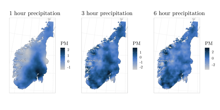
Figure 2: Estimated posterior mean (PM) of the Gaussian field $u_{\mu}(\bm{s})$ for three different temporal aggregations of precipitation, with unit mm.

The posterior distribution of $\xi$ is also described in Table 4. The tail parameter seems to decrease quickly as the aggregation time increases, and it is practically constant for precipitation over longer periods than 12 hours. This makes sense given the observation of [2] that most 24 hour annual maximum precipitation comes from rainstorms with lengths of less than 15 hours. Thus, the tail parameter for 24 hour precipitation should be close to the tail parameter for 12 hour precipitation. For 12 hours and up, the tail parameter is so small that one may wonder if a Gumbel distribution would not have given a better fit to the data. However, this is not the case for the shorter aggregation times, where the tail parameter is considerably larger.

4.4 Return levels

We use the two-step model for estimating large return levels for the yearly precipitation maxima. Posterior distributions of the 20 year return levels are estimated on a grid with resolution $1\times 1$ km². The posterior means and the widths of the $95\%$ credible intervals are displayed in Figure 3. For a period of 1 hour the most extreme precipitation is located southeast in Norway, while for longer periods, the extreme precipitation is moving over to the west coast. These results are expected since we know that the convective precipitation of the southeast dominates for short aggregation periods. At the same time, the southwest of Norway generally has more precipitation, making it the dominant region for longer aggregation times. The spatial structure and magnitude of the 20 year return levels for hourly precipitation are similar to the estimates of [19], but with considerably thinner credible intervals. This makes sense as more data are available, and the two-step model is able to perform less wasteful inference. In addition, our model is much more simple, as they include a random Gaussian field in all three parameters, while we only include a random Gaussian field in the location parameter. This can also lead to less uncertainty in the return level estimates.

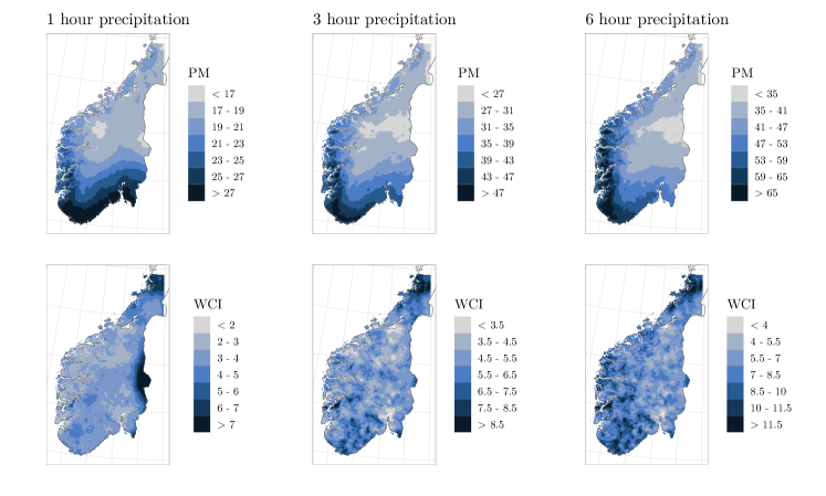
Figure 3: Estimated posterior mean (PM) and width of the $95\%$ credible intervals (WCI) for the 20 year return levels of sub-daily precipitation. Different aggregation times are displayed in different columns. All numbers are given with unit mm.

5 Conclusion

The blended generalised extreme value (bGEV) distribution is applied as a substitute for the generalised extreme value (GEV) distribution for estimation of the return levels of sub-daily precipitation in the south of Norway. The bGEV distribution simplifies inference by introducing a parameter-free support, but can only be applied for modelling of heavy-tailed phenomena. Sub-daily precipitation maxima are modelled using a spatial Bayesian hierarchical model with a latent Gaussian field. This is implemented using both integrated nested Laplace approximations (INLA) and the stochastic partial differential equation (SPDE) approach, for fast inference. Inference is also made more stable and less wasteful by our novel two-step modelling procedure that borrows strength from the peaks over threshold method when modelling block maxima. Like the GEV distribution, the bGEV distribution suffers from a lack of log-concavity, which can cause problems when using INLA. We are able to mitigate any problems caused by a lack of log-concavity by choosing slightly informative priors and standardising the data. We find that the bGEV distribution performs well as a model for extreme precipitation. The two-step model successfully utilises the additional information provided by the peaks over threshold data and is able to outperform models that only use block maxima data for inference.

Funding

This publication is part of the World of Wild Waters (WoWW) project, which falls under the umbrella of Norwegian University of Science and Technology (NTNU)’s Digital Transformation initiative.

Code and data availability

The necessary code and data for achieving these results are available online at https://github.com/siliusmv/inlaBGEV. The unprocessed data are freely available online, as described in Section 2.

Conflicts of interest

The authors declare that they have no conflicts of interest.

Supplementary material

Appendix S1 Simulation study

A simulation study is conducted for comparing the performance of the generalised extreme value (GEV) distribution and blended generalised extreme value (bGEV) distribution in a univariate setting. Our penultimate goal when modelling block maxima is to estimate return levels. Thus, the two distributions are compared by evaluating the performance of their return level estimators.

We sample $n\in\{25,50,100,500,1000\}$ i.i.d. “block maxima” from a GEV distribution resembling the estimated distribution of the yearly maxima of hourly precipitation. From Table 3 and Table 4 in “Modelling sub-daily precipitation extremes with the blended generalised extreme value distribution” we find that the posterior mean of the intercept in $\bm{\beta}_{\mu}$ is $E[\beta_{\mu,0}]=0.661$, and the posterior mean of the intercept in $\bm{\beta}_{\sigma}$ is $E[\beta_{\sigma,0}]=2.835$. Consequently, we set $\alpha=0.5$, $\beta=0.8$, $\mu_{\alpha}=E[\beta_{\mu,0}]\cdot\exp(E[\beta_{\sigma,0}])\approx 11.26$, and $\sigma_{\beta}=E[\sigma_{\beta}^{*}]\cdot\exp(E[\beta_{\sigma,0}])\approx 2.01$. The tail parameter is set equal to the posterior mean from Table 4: $\xi=0.178$. Using the $n$ block maxima, we compute maximum likelihood estimators for the parameters of the GEV and bGEV distributions, which are further used for computing return level estimators for periods of length 25, 50, 100, 250 and 500. The actual maximum likelihood estimation is performed on the $(\mu,\sigma,\xi)$ parametrisation, in which $\mu\approx 10.05$ and $\sigma\approx 3.21$. Optimisation is performed using the optim function in R, where the true values of $(\mu,\sigma,\xi)$ are used as initial values. The entire procedure is repeated 500 times for each value of $n$. This allows us to estimate the distribution of the maximum likelihood estimators for all return levels in question.

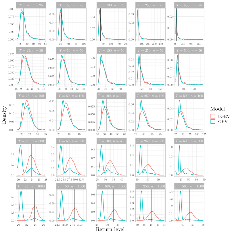
Figure S1.1: Distributions of return level estimators computed from model fits with the GEV and bGEV distributions to simulated data from a GEV distribution. The dark vertical lines display the true return levels. Return periods are denoted as $T$, with unit “block sizes”, and the number of block maxima used for fitting the GEV and bGEV distributions is denoted as $n$.

Figure S1.1 displays the distribution of all return level estimators using both the GEV and the bGEV distributions. The difference between the distributions of the GEV estimators and the bGEV estimators are negligible for small values of $n$. For large return periods and values of $n$ some slight differences are appearing. However, in practical situations one rarely encounters as much as 1000 block maxima, and the blocks are almost never large enough for the limit distribution to hold exactly. Thus, the differences in distribution can be considered negligible for large values of $n$ for almost all real-life settings. Larger differences in model fit could theoretically occur for small blocks where the block maxima deviate further from the GEV distribution. However, in such settings, both the GEV and the bGEV distribution would be misspecified, and we have no reason to believe that the misspecification in the GEV distribution would be strictly better or worse than the misspecification in the bGEV distribution. Therefore, our results imply that we do not lose anything in performance by modelling GEV data with the bGEV distribution instead of the GEV distribution.

In most real-life settings we do not have as much prior knowledge about the true underlying distribution, and we will likely choose less optimal initial values and/or prior distributions. To examine the effects of choosing less optimal initial values, we repeat the maximum likelihood estimation on the exact same data used for Figure S1.1, using different initial values. Figure S1.2 displays the distributions of the return level estimators when we use an initial value of $0.9$ instead of $3.2$ for $\sigma$, without changing the initial values for $\mu$ or $\xi$. For small values of $n$ the two distributions yield comparable results. However, for large values of $n$, the performance of the GEV distribution quickly deteriorates, and the return level estimators are shifted to the left. The bGEV estimators, however, seem to have identical distributions in Figures S1.1 and S1.2, and are not affected by the slight change of initial values. This demonstrates how inference with the bGEV distribution is more robust than inference with the GEV distribution. The parameter-dependent support of the GEV complicates likelihood-based inference and makes it more difficult to locate the global maximum of the likelihood, even in simple and univariate settings with unrealistically large amounts of data that are perfectly GEV-distributed.

In such a simple setting, it is relatively easy to see that we chose bad initial values for $(\mu,\sigma,\xi)$. However, when modelling block maxima with a large number of covariates and in high-dimensional settings, it becomes considerably more difficult to choose good enough initial values and/or prior distributions. Additionally, it is not trivial to examine a maximum likelihood estimator or posterior distribution and find out if the inference procedure was successful or not. The GEV return level estimators in Figure S1.2 take on reasonable values and are large enough to seem realistic. Without knowing the truth, it would not be trivial for a practitioner to detect that they are faulty, and caused by numerical problems. Thus, if one performs likelihood-based inference using the GEV distribution, one should always perform extensive checks to evaluate whether the fit is reasonable, or if it is caused by numerical problems. The increased robustness of the bGEV distribution provides more safety, and most practitioners can be more confident in their model fits after fitting the bGEV distribution to block maxima data instead of the GEV distribution.

Similarly, while attempting to model return levels for precipitation in Norway using the gev family in R-INLA, we experienced that e.g. adding or removing one covariate from the model could completely alter the model fits if our priors were too wide or the data were not correctly standardised. Examining which of the fits were the best required comprehensive and time-demanding cross-validation studies, and it was difficult to find out if the best model fit was “good enough”, or if a slight change in priors or covariates would yield considerably better model fits. These problems were considerably mitigated by switching to the bgev family, which resulted in more stable inference using less informative priors, and less optimal initial values.

Figure S1.2: Distributions of return level estimators computed from model fits with the GEV and bGEV distributions to simulated data from a GEV distribution, when using bad initial values. The dark vertical lines display the true return levels. Return periods are denoted as $T$, with unit “block sizes”, and the number of block maxima used for fitting the GEV and bGEV distributions is denoted as $n$.

Appendix S2 PC prior for the tail parameter

In order to compute the PC prior for the GEV and bGEV distribution with $\xi\geq 0$ and base model $\xi=0$, one must first compute KLD$(\pi_{\xi},\pi_{0})$ for the GEV distribution and the bGEV distribution. Notice that the base model is identical for both distributions. Writing the GEV distribution function as $F(x)=\exp(-h(x))$ gives the probability density function

$$\pi_{\xi}(x)=-\exp(-h(x))h^{\prime}(x),\quad h(x)=(1+\xi(x-\mu)/\sigma)^{-1/\xi}_{+}.$$

The KLD for the GEV distribution is equal to

$$\text{KLD}(\pi_{\xi},\pi_{0})= \int\pi_{\xi}(x)\log\left(\frac{\pi_{\xi}(x)}{\pi_{0}(x)}\right)\text{d}x$$

$$= \int-e^{-h(x)}h^{\prime}(x)\cdot\left(-h(x)+\log(-\sigma h^{\prime}(x))+\exp\left(-\frac{x-\mu}{\sigma}\right)+\frac{x-\mu}{\sigma}\right)\text{d}x.$$

The fourth term of the KLD is simply equal to the expectation of $(x-\mu)/\sigma$, which is known. The first term is easily solvable with the substitution $u=h(x)$. Using the same substitution for the second term with the knowledge that $\log(-\sigma h^{\prime}(x))=(1+\xi)\log(h(x))$ gives the integral

$$\int-e^{-h(x)}h^{\prime}(x)\log(-\sigma h^{\prime}(x))=\int_{0}^{\infty}e^{-u}(1+\xi)\log(u)\ \text{d}u=-(1+\xi)\gamma,$$

where $\gamma$ is the Euler-Mascheroni constant. We are unable to find a closed-form expression for the third term. However, using substitution with $u=h(x)$ gives

$$\int-e^{-h(x)}h^{\prime}(x)\exp\left(-\frac{x-\mu}{\sigma}\right)\text{d}x=\int_{0}^{\infty}\exp\left(\frac{1}{\xi}-u-\frac{u^{-\xi}}{\xi}\right)\text{d}u,$$

which is finite for $\xi>0$. With a change of variables, this integral is transformed to have finite limits,

$$\int_{0}^{\infty}\exp\left(\frac{1}{\xi}-\left(u+u^{-\xi}/\xi\right)\right)\text{d}u=\int_{0}^{1}\exp\left(\frac{1}{\xi}\left(1-(-\log v)^{-\xi}\right)\right)\text{d}v.$$

This can easily be numerically approximated. Summarising, the KLD for the GEV is finite for $0\leq\xi<1$ and equal to

$$\text{KLD}(\pi_{\xi},\pi_{0})=-1-(1+\xi)\gamma+\xi^{-1}(\Gamma(1-\xi)-1)+\int_{0}^{1}\exp\left(\frac{1}{\xi}\left(1-(-\log v)^{-\xi}\right)\right)\text{d}v.$$ (S2.1)

The PC prior has probability density function $\pi(d)=\lambda\exp(-\lambda d)$ with $d=\sqrt{2\text{KLD}(\pi_{\xi},\pi_{0})}$. Transforming the PC prior from a distribution on $d$ to a distribution on $\xi$ gives

$$\pi(\xi)=\lambda\exp\left(-\lambda d(\xi)\right)\left|\frac{\partial d(\xi)}{\partial\xi}\right|=\frac{\lambda}{d(\xi)}\exp\left(-\lambda d(\xi)\right)\left|\frac{\partial}{\partial\xi}\text{KLD}(\pi_{\xi},\pi_{0})\right|.$$ (S2.2)

Consequently, the derivative of the KLD must also be computed. Using derivation under the integral sign gives

$$\frac{\partial}{\partial\xi}\text{KLD}(\pi_{\xi},\pi_{0})=-\gamma-\frac{\Gamma(1-\xi)\Psi(1-\xi)}{\xi}-\frac{\Gamma(1-\xi)-1}{\xi^{2}}+\int_{0}^{1}g(v;\xi)\text{d}v,$$

where $\Psi(\cdot)$ is the digamma function, and

$$g(v;\xi)=\exp\left(\frac{1}{\xi}\left(1-(-\log v)^{-\xi}\right)\right)\frac{1}{\xi^{2}}\left(-1+(-\log v)^{-\xi}\left(1+\xi\log(-\log v)\right)\right).$$

This integral must also be numerically approximated.

When computing the KLD for the bGEV distribution, the integral for the KLD is divided into three parts:

$$\text{KLD}(\pi_{\xi},\pi_{0})=$$

$$\qquad\int_{-\infty}^{p_{a}}\pi_{\xi}(x)\log\left(\frac{\pi_{\xi}(x)}{\pi_{0}(x)}\right)\text{d}x+\int_{p_{a}}^{p_{b}}\pi_{\xi}(x)\log\left(\frac{\pi_{\xi}(x)}{\pi_{0}(x)}\right)\text{d}x+\int_{p_{b}}^{\infty}\pi_{\xi}(x)\log\left(\frac{\pi_{\xi}(x)}{\pi_{0}(x)}\right)\text{d}x$$

$$\qquad=\text{KLD}_{\text{Gumbel}}(\pi_{\xi},\pi_{0})+\text{KLD}_{\text{Blending}}(\pi_{\xi},\pi_{0})+\text{KLD}_{\text{Fréchet}}(\pi_{\xi},\pi_{0}).$$

A closed-form expression can be found for the Gumbel part of the KLD, where we express the Gumbel distribution function as $G(x)=\exp(-h_{2}(x))$ and use the same substitution techniques as for the KLD computations with the GEV distribution. We get

$$\text{KLD}_{\text{Gumbel}}(\pi_{\xi},\pi_{0})=$$

$$\qquad-\Gamma_{u}(-\log p_{a};2)+p_{a}\log(-\log p_{a})-E_{i}(\log p_{a})+\Gamma_{u}(-\log p_{a};C_{1}+1)e^{-C_{2}}$$

$$\qquad-C_{1}\left(p_{a}\log(-\log p_{a})-E_{i}(\log p_{a})\right)+p_{a}\left(C_{2}+\log\xi+\log\left(\log\left(\frac{\log p_{a}}{\log p_{b}}\right)\right)\right)$$

$$\qquad-p_{a}\log\left((-\log p_{b})^{-\xi}-(-\log p_{a})^{-\xi}\right),$$

where

$$C_{1}=\frac{1}{\xi}\frac{(-\log p_{b})^{-\xi}-(-\log p_{a})^{-\xi}}{\log\left(\frac{\log p_{a}}{\log p_{b}}\right)}\quad\text{and}\quad C_{2}=C_{1}\log(-\log p_{a})+\frac{1}{\xi}\left((-\log p_{a})^{-\xi}-1\right).$$

Here, $\Gamma_{u}(x;\alpha)=\int_{x}^{\infty}t^{\alpha-1}e^{-t}\text{d}t$ is the upper incomplete gamma function, and $E_{i}(x)=\int_{-\infty}^{x}(e^{t}/t)\text{d}t$ is the exponential integral, which can be evaluated using the GNU Scientific Library [24, 29]. The Fréchet part of the KLD is found in the same way as (S2.1), only using different integration limits. For $0\leq\xi<1$ we get

$$\text{KLD}_{\text{Fréchet}}(\pi_{\xi},\pi_{0})= -\Gamma_{l}(-\log p_{b};2)+(\xi+1)\left(-p_{b}\log(-\log p_{b})+E_{i}(\log p_{b})-\gamma\right)$$

$$+\frac{1}{\xi}\left(\Gamma_{l}(-\log p_{b};1-\xi)-(1-p_{b})\right)+\int_{p_{b}}^{1}\exp\left(\frac{1}{\xi}\left(1-(-\log u)^{-\xi}\right)\right)\text{d}u,$$

where $\Gamma_{l}(x;\alpha)=\Gamma(\alpha)-\Gamma_{u}(x;\alpha)$ is the lower incomplete gamma function. The integral in the expression above must once again be evaluated numerically. We are unable to find an expression for the KLD integral between the $p_{a}$ quantile and the $p_{b}$ quantile. Thus, we use numerical integration with $\mu=0$ and $\sigma=1$ to compute $\text{KLD}_{\text{Blending}}(\pi_{\xi},\pi_{0})$. The value of the integral does not depend on the values of $\mu$ and $\sigma$, but we are unable to compute it without choosing some value for them. Being unable to find an expression for the KLD of the bGEV distribution, we must also use numerical derivation to estimate the derivative of the KLD, needed in (S2.2).

The PC priors for the GEV, bGEV and generalised Pareto distributions are displayed in Figure S2.1 for different values of the penalty parameter $\lambda$. For all the chosen values of $\lambda$ the three distributions are so similar that their effect on a posterior distribution probably will be close to identical. The PC prior for the generalised Pareto distribution exists in closed-form and is already implemented in R-INLA, while the other PC priors must be computed numerically and are not implemented in R-INLA. Consequently, we choose to use the PC prior of the generalised Pareto distribution for modelling the tail parameter of the bGEV distribution.

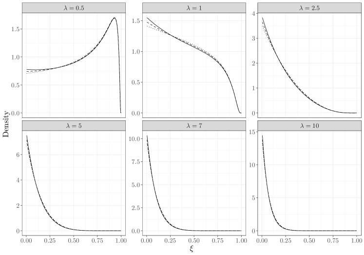
Figure S2.1: PC priors with base models $\xi=0$ and different penalty parameters $\lambda$ for the GEV (solid line), bGEV (dashed line) and generalised Pareto distribution (dotted line).

References

- [1] Haakon Bakka et al. “Spatial Modeling With R-INLA: a Review” In WIREs Comput. Stat. 10.6, 2018, pp. e1443 DOI: 10.1002/wics.1443
- [2] Renaud Barbero et al. “A Synthesis of Hourly and Daily Precipitation Extremes in Different Climatic Regions” In Weather Clim. Extremes 26, 2019, pp. 100219 DOI: 10.1016/j.wace.2019.100219
- [3] Roger Bivand, Virgilio Gómez-Rubio and Håvard Rue “Spatial Data Analysis with R-INLA with Some Extensions” In Journal of Statistical Software 63.1 Directory of Open Access Journals, 2015, pp. 1–31
- [4] David Bolin and Jonas Wallin “Scale Dependence: Why the Average CRPS Often Is Inappropriate for Ranking Probabilistic Forecasts” In arXiv:1912.05642, 2019
- [5] Axel Bücher and Johan Segers “On the Maximum Likelihood Estimator for the Generalized Extreme-Value Distribution” In Extremes 20.4, 2017, pp. 839–872 DOI: 10.1007/s10687-017-0292-6
- [6] Axel Bücher and Johan Segers “Inference for Heavy Tailed Stationary Time Series Based on Sliding Blocks” In Electronic Journal of Statistics 12.1 Institute of Mathematical StatisticsBernoulli Society, 2018, pp. 1098–1125 DOI: 10.1214/18-EJS1415
- [7] Axel Bücher and Chen Zhou “A Horse Race Between the Block Maxima Method and the Peak-Over-Threshold Approach” In Statistical Science 36.3 Institute of Mathematical Statistics, 2021, pp. 360–378 DOI: 10.1214/20-STS795
- [8] Julie Carreau, Philippe Naveau and Luc Neppel “Characterization of homogeneous regions for regional peaks-over-threshold modeling of heavy precipitation” working paper or preprint, 2016 URL: https://hal.ird.fr/ird-01331374
- [9] Daniela Castro-Camilo and Raphaël Huser “Local Likelihood Estimation of Complex Tail Dependence Structures, Applied To U.S. Precipitation Extremes” In J. Amer. Statist. Assoc. 115.531 Taylor & Francis, 2020, pp. 1037–1054 DOI: 10.1080/01621459.2019.1647842
- [10] Daniela Castro-Camilo, Raphaël Huser and Håvard Rue “A Spliced Gamma-Generalized Pareto Model for Short-Term Extreme Wind Speed Probabilistic Forecasting” In JABES 24.3, 2019, pp. 517–534 DOI: 10.1007/s13253-019-00369-z
- [11] Daniela Castro-Camilo, Raphaël Huser and Håvard Rue “Practical Strategies for GEV-based Regression Models for Extremes” arXiv, 2021 DOI: 10.48550/ARXIV.2106.13110
- [12] Stuart Coles “An Introduction to Statistical Modeling of Extreme Values” Springer, London, 2001 DOI: 10.1007/978-1-4471-3675-0
- [13] Daniel Cooley, Douglas Nychka and Philippe Naveau “Bayesian Spatial Modeling of Extreme Precipitation Return Levels” In J. Amer. Statist. Assoc. 102.479 Taylor & Francis, 2007, pp. 824–840 DOI: 10.1198/016214506000000780
- [14] Alice Crespi et al. “High-Resolution Monthly Precipitation Climatologies Over Norway: Assessment of Spatial Interpolation Methods” In arXiv:1804.04867, 2018
- [15] Tate Dalrymple “Flood-frequency analyses” U.S. Government Printing Office, 1960
- [16] A.. Davison and R. Huser “Statistics of Extremes” In Annu. Rev. Stat. Appl. 2.1, 2015, pp. 203–235 DOI: 10.1146/annurev-statistics-010814-020133
- [17] A.. Davison, S.. Padoan and M. Ribatet “Statistical Modeling of Spatial Extremes” In Statist. Sci. 27.2 The Institute of Mathematical Statistics, 2012, pp. 161–186 DOI: 10.1214/11-STS376
- [18] A.. Davison and R.. Smith “Models for Exceedances Over High Thresholds” In J. R. Stat. Soc. B 52.3, 1990, pp. 393–425 DOI: 10.1111/j.2517-6161.1990.tb01796.x
- [19] Anita Verpe Dyrrdal, Alex Lenkoski, Thordis L. Thorarinsdottir and Frode Stordal “Bayesian Hierarchical Modeling of Extreme Hourly Precipitation in Norway” In Environmetrics 26.2, 2015, pp. 89–106 DOI: 10.1002/env.2301
- [20] Anita Verpe Dyrrdal, Thomas Skaugen, Frode Stordal and Eirik J. Førland “Estimating Extreme Areal Precipitation in Norway From a Gridded Dataset” In Hydrol. Sci. J. 61.3 Taylor & Francis, 2016, pp. 483–494 DOI: 10.1080/02626667.2014.947289
- [21] R.. Fisher and L… Tippett “Limiting Forms of the Frequency Distribution of the Largest Or Smallest Member of a Sample” In Math. Proc. Cambridge Philos. Soc. 24.2 Cambridge University Press, 1928, pp. 180–190 DOI: 10.1017/S0305004100015681
- [22] Petra Friederichs and Thordis L. Thorarinsdottir “Forecast Verification for Extreme Value Distributions With an Application To Probabilistic Peak Wind Prediction” In Environmetrics 23.7, 2012, pp. 579–594 DOI: 10.1002/env.2176
- [23] Geir-Arne Fuglstad, Daniel Simpson, Finn Lindgren and Håvard Rue “Constructing Priors That Penalize the Complexity of Gaussian Random Fields” In J. Amer. Statist. Assoc. 114.525 Taylor & Francis, 2019, pp. 445–452 DOI: 10.1080/01621459.2017.1415907
- [24] Mark Galassi et al. “The GNU Scientific Library Reference Manual, 2007”, 2007 URL: http://www.gnu.org/software/gsl
- [25] Óli P. Geirsson, Birgir Hrafnkelsson and Daniel Simpson “Computationally Efficient Spatial Modeling of Annual Maximum 24-h Precipitation on a Fine Grid” In Environmetrics 26.5, 2015, pp. 339–353 DOI: 10.1002/env.2343
- [26] Tilmann Gneiting and Adrian E Raftery “Strictly Proper Scoring Rules, Prediction, and Estimation” In J. Amer. Statist. Assoc. 102.477 Taylor & Francis, 2007, pp. 359–378 DOI: 10.1198/016214506000001437
- [27] Tilmann Gneiting and Roopesh Ranjan “Comparing Density Forecasts Using Threshold- and Quantile-Weighted Scoring Rules” In J. Bus. Econ. Stat. 29.3 Taylor & Francis, 2011, pp. 411–422 DOI: 10.1198/jbes.2010.08110
- [28] Peter Guttorp and Tilmann Gneiting “Studies in the History of Probability and Statistics XLIX on the Matérn Correlation family” In Biometrika 93.4, 2006, pp. 989–995 DOI: 10.1093/biomet/93.4.989
- [29] Robin K.. Hankin “Special Functions in R: Introducing the Gsl Package” In R News 6, 2006
- [30] I. Hanssen-Bauer and E.. Førland “Annual and seasonal precipitation variations in Norway 1896-1997” In DNMI KLIMA Report 27/98, 1998
- [31] Jonathan Richard Morley Hosking and James R Wallis “Regional frequency analysis”, 1997
- [32] Richard W Katz, Marc B Parlange and Philippe Naveau “Statistics of Extremes in Hydrology” In Adv. Water Res. 25.8, 2002, pp. 1287–1304 DOI: 10.1016/S0309-1708(02)00056-8
- [33] Roger Koenker “Quantile regression” 38, Econometric Society monographs ;, 2005 DOI: 10.1017/CBO9780511754098
- [34] Roger Koenker “quantreg: Quantile Regression” R package version 5.75, 2020 URL: https://CRAN.R-project.org/package=quantreg
- [35] Demetris Koutsoyiannis, Demosthenes Kozonis and Alexandros Manetas “A Mathematical Framework for Studying Rainfall Intensity-Duration-Frequency Relationships” In Journal of Hydrology 206.1, 1998, pp. 118–135 DOI: 10.1016/S0022-1694(98)00097-3
- [36] Eric A. Lehmann, Aloke Phatak, Alec Stephenson and Rex Lau “Spatial Modelling Framework for the Characterisation of Rainfall Extremes At Different Durations and Under Climate Change” In Environmetrics 27.4, 2016, pp. 239–251 DOI: 10.1002/env.2389
- [37] Sebastian Lerch, Thordis L. Thorarinsdottir, Francesco Ravazzolo and Tilmann Gneiting “Forecaster’s Dilemma: Extreme Events and Forecast Evaluation” In Statist. Sci. 32.1 The Institute of Mathematical Statistics, 2017, pp. 106–127 DOI: 10.1214/16-STS588
- [38] Finn Lindgren and Håvard Rue “Bayesian Spatial Modelling With R-INLA” In J Stat Softw 63.19 University of California at Los Angeles, 2015
- [39] Finn Lindgren, Håvard Rue and Johan Lindström “An Explicit Link Between Gaussian Fields and Gaussian Markov Random Fields: the Stochastic Partial Differential Equation Approach” In J. R. Stat. Soc. B 73.4, 2011, pp. 423–498 DOI: 10.1111/j.1467-9868.2011.00777.x
- [40] C Lussana et al. “seNorge2 Daily Precipitation, an Observational Gridded Dataset Over Norway From 1957 To the Present Day” In Earth Syst. Sci. Data 10.1 Copernicus GmbH, 2018, pp. 235 DOI: 10.5194/essd-10-235-2018
- [41] C Lussana, OE Tveito and F Uboldi “Three-Dimensional Spatial Interpolation of 2 M Temperature Over Norway” In Q. J. R. Meteorolog. Soc. 144.711 Wiley Online Library, 2018, pp. 344–364 DOI: 10.1002/qj.3208
- [42] B Matern “Spatial Variation” 36, Lecture Notes in Statistics New York, NY: Springer New York : Imprint: Springer, 1986 DOI: 10.1007/978-1-4615-7892-5
- [43] James E. Matheson and Robert L. Winkler “Scoring Rules for Continuous Probability Distributions” In Manage Sci 22.10, 1976, pp. 1087–1096 DOI: 10.1287/mnsc.22.10.1087
- [44] Matthias Mohr “Comparison of Versions 1.1 and 1.0 of Gridded Temperature and Precipitation Data for Norway” In met.no note 19, 2009
- [45] P. Naveau, A. Toreti, I. Smith and E. Xoplaki “A Fast Nonparametric Spatio-Temporal Regression Scheme for Generalized Pareto Distributed Heavy Precipitation” In Water Resources Research 50.5, 2014, pp. 4011–4017 DOI: 10.1002/2014WR015431
- [46] Thomas Opitz, Raphaël Huser, Haakon Bakka and Håvard Rue “INLA Goes Extreme: Bayesian Tail Regression for the Estimation of High Spatio-Temporal Quantiles” In Extremes 21.3, 2018, pp. 441–462 DOI: 10.1007/s10687-018-0324-x
- [47] Simon Michael Papalexiou and Demetris Koutsoyiannis “Battle of Extreme Value Distributions: a Global Survey on Extreme Daily Rainfall” In Water Resour. Res. 49.1, 2013, pp. 187–201 DOI: 10.1029/2012WR012557
- [48] M.. Robinson and J.. Tawn “Extremal Analysis of Processes Sampled At Different Frequencies” In J. R. Stat. Soc. B 62.1, 2000, pp. 117–135 DOI: 10.1111/1467-9868.00223
- [49] Håvard Rue, Sara Martino and Nicolas Chopin “Approximate Bayesian Inference for Latent Gaussian Models By Using Integrated Nested Laplace Approximations” In J. R. Stat. Soc. B 71.2, 2009, pp. 319–392 DOI: 10.1111/j.1467-9868.2008.00700.x
- [50] Håvard Rue et al. “Bayesian Computing With INLA: a Review” In Annu. Rev. Stat. Appl. 4.1, 2017, pp. 395–421 DOI: 10.1146/annurev-statistics-060116-054045
- [51] Huiyan Sang and Alan Gelfand “Continuous Spatial Process Models for Spatial Extreme Values” In J. Agric. Biol. Environ. Stat. 15, 2010, pp. 49–65 DOI: 10.1007/s13253-009-0010-1
- [52] Huiyan Sang and Alan E. Gelfand “Hierarchical Modeling for Extreme Values Observed Over Space and Time” In Environ. Ecol. Stat. 16.3, 2009, pp. 407–426 DOI: 10.1007/s10651-007-0078-0
- [53] Daniel Simpson et al. “Penalising Model Component Complexity: a Principled, Practical Approach To Constructing Priors” In Statist. Sci. 32.1 The Institute of Mathematical Statistics, 2017, pp. 1–28 DOI: 10.1214/16-STS576
- [54] Richard L. Smith “Maximum Likelihood Estimation in a Class of Nonregular cases” In Biometrika 72.1, 1985, pp. 67–90 DOI: 10.1093/biomet/72.1.67
- [55] Michael L Stein “Interpolation of spatial data : some theory for Kriging”, Springer series in statistics New York: Springer, 1999
- [56] Ying Sun, Kenneth P. Bowman, Marc G. Genton and Ali Tokay “A Matérn Model of the Spatial Covariance Structure of Point Rain Rates” In Stoch Env Res Risk A 29.2, 2015, pp. 411–416 DOI: 10.1007/s00477-014-0923-2
- [57] Ole Einar Tveito, Inge Bjørdal, Arne Oddvar Skjelvåg and Bjørn Aune “A GIS-Based Agro-Ecological Decision System Based on Gridded Climatology” In Meteorol Appl 12.1, 2005, pp. 57–68 DOI: 10.1017/S1350482705001490
- [58] Jana Ulrich et al. “Estimating IDF Curves Consistently Over Durations With Spatial Covariates” In Water 12.11, 2020 DOI: 10.3390/w12113119
- [59] H. Van de Vyver “Spatial Regression Models for Extreme Precipitation in Belgium” In Water Resour. Res. 48.9, 2012 DOI: 10.1029/2011WR011707
- [60] Silius M. Vandeskog, Sara Martino and Daniela Castro-Camilo “Modelling Block Maxima with the blended generalised extreme value distribution” In 22nd European Young Statisticians Meeting - Proceedings, 2021
- [61] Yixin Wang and Mike K.P. So “A Bayesian Hierarchical Model for Spatial Extremes With Multiple Durations” In Computational Statistics & Data Analysis 95, 2016, pp. 39–56 DOI: 10.1016/j.csda.2015.09.001
- [62] P. Whittle “On Stationary Processes in the Plane” In Biometrika 41.3/4 [Oxford University Press, Biometrika Trust], 1954, pp. 434–449 URL: http://www.jstor.org/stable/2332724
- [63] P.. Wilson and R. Toumi “A Fundamental Probability Distribution for Heavy Rainfall” In Geophys. Res. Lett. 32.14, 2005 DOI: 10.1029/2005GL022465
- [64] World Economic Forum “The Global Risks Report 2021”, 2021 URL: http://www3.weforum.org/docs/WEF_The_Global_Risks_Report_2021.pdf
- [65] Nan Zou, Stanislav Volgushev and Axel Bücher “Multiple Block Sizes and Overlapping Blocks for Multivariate Time Series Extremes” In arXiv:1907.09477, 2019 arXiv:1907.09477 [math.ST]