Reduced Sum Implementation of the BURA Method for Spectral Fractional Diffusion Problems

Abstract

The numerical solution of spectral fractional diffusion problems in the form ${\mathcal{A}}^{\alpha}u=f$ is studied, where $\mathcal{A}$ is a selfadjoint elliptic operator in a bounded domain $\Omega\subset{\mathbb{R}}^{d}$, and $\alpha\in(0,1]$. The finite difference approximation of the problem leads to the system ${\mathbb{A}}^{\alpha}{\mathbf{u}}={\mathbf{f}}$, where ${\mathbb{A}}$ is a sparse, symmetric and positive definite (SPD) matrix, and ${\mathbb{A}}^{\alpha}$ is defined by its spectral decomposition. In the case of finite element approximation, ${\mathbb{A}}$ is SPD with respect to the dot product associated with the mass matrix. The BURA method is introduced by the best uniform rational approximation of degree $k$ of $t^{\alpha}$ in $[0,1]$, denoted by $r_{\alpha,k}$. Then the approximation ${\bf u}_{k}\approx{\bf u}$ has the form ${\bf u}_{k}=c_{0}{\mathbf{f}}+\sum_{i=1}^{k}c_{i}({\mathbb{A}}-{\widetilde{d}}_{i}{\mathbb{I}})^{-1}{\mathbf{f}}$, ${\widetilde{d}}_{i}<0$, thus requiring the solving of $k$ auxiliary linear systems with sparse SPD matrices. The BURA method has almost optimal computational complexity, assuming that an optimal PCG iterative solution method is applied to the involved auxiliary linear systems. The presented analysis shows that the absolute values of first $\left\{{\widetilde{d}}_{i}\right\}_{i=1}^{k^{\prime}}$ can be extremely large. In such a case the condition number of ${\mathbb{A}}-{\widetilde{d}}_{i}{\mathbb{I}}$ is practically equal to one. Obviously, such systems do not need preconditioning. The next question is if we can replace their solution by directly multiplying ${\mathbf{f}}$ with $-c_{i}/{\widetilde{d}}_{i}$. Comparative analysis of numerical results is presented as a proof-of-concept for the proposed RS-BURA method.

1 Introduction

We consider the second order elliptic operator ${\mathcal{A}}$ in the bounded domain $\Omega\subset{\mathbb{R}}^{d}$, $d\in\{1,2,3\}$, assuming homogeneous boundary conditions on $\partial\Omega$. Let $\{\lambda_{j},\psi_{j}\}_{j=1}^{\infty}$ be the eigenvalues and eigenfunctions of $\mathcal{A}$, and let $(\cdot,\cdot)$ stand for the $L^{2}$ dot product. The spectral fractional diffusion problem ${\mathcal{A}}^{\alpha}u=f$ is defined by the equality

$$\mathcal{A}^{\alpha}u=\sum_{j=1}^{\infty}\lambda_{j}^{\alpha}(u,\psi_{j})\psi_{j},~{}~{}\mbox{and therefore}~{}~{}u=\sum_{j=1}^{\infty}\lambda_{j}^{-\alpha}(f,\psi_{j})\psi_{j}.$$ (1)

Now, let a $(2d+1)$-point stencil on a uniform mesh be used to get the finite difference (FDM) approximation of $\mathcal{A}$. Then, the FDM numerical solution of (1) is given by the linear system

$$\mathbb{A}^{\alpha}{\bf u}={\bf f},$$ (2)

where ${\bf u}$ and ${\bf f}$ are the related mesh-point vectors, $\mathbb{A}\in\mathbb{R}^{N\times N}$ is SPD matrix, and $\mathbb{A}^{\alpha}$ is defined similarly to (1), using the spectrum $\{\lambda_{j,h},\Psi_{j,h}\}_{j=1}^{N}$ of $\mathbb{A}$.

Alternatively, the finite element method (FEM) can be applied for the numerical solution of the fractional diffusion problem, if $\Omega$ is a general domain and some unstructured (say, triangular or tetrahedral) mesh is used. Then, $\mathbb{A}=\mathbb{M}^{-1}\mathbb{K}$, where $\mathbb{K}$ and $\mathbb{M}$ are the stiffness and mass matrices respectively, and $\mathbb{A}$ is SPD with respect to the energy dot product associated with $\mathbb{M}$.

Rigorous error estimates for the linear FEM approximation of (1) are presented in [1]. More recently, the mass lumping case is analyzed in [6]. The general result is that the relative accuracy in $L^{2}$ behaves essentially as $O(h^{2\alpha})$ for both linear FEM or $(2d+1)$-point stencil FDM discretizations.

A survey on the latest achievements in numerical methods for fractional diffusion problems is presented in [4]. Although there are several different approaches discussed there, all the derived algorithms can be interpreted as rational approximations, see also [7]. In this context, the advantages of the BURA (best uniform rational approximation) method are reported. The BURA method is originally introduced in [5], see [6] and the references therein for some further developments. The method is generalized to the case of Neumann boundary conditions in [3]. The present study is focused on the efficient implementation of the method for large-scale problems, where preconditioned conjugate gradient (PCG) iterative solver of optimal complexity is applied to the arising auxiliary sparse SPD linear systems.

The rest of the paper is organized as follows. The construction and some basic properties of the BURA method are presented in Section 2. The numerical stability of computing the BURA parameters is discussed in Section 3. The next section is devoted to the question how large can the BURA coefficients be, followed by the introduction of the new RS-BURA method based on reduced sum implementation in Section 5. A comparative analysis of the accuracy is provided for the considered test problem ($\alpha=0.25$, $k=85$ and reduced sum of $46$ terms), varying the parameter $\delta$, corresponding to the spectral condition number of $\mathbb{A}$. Brief concluding remarks are given at the end.

2 The BURA Method

Let us consider the min-max problem

$$\min_{r_{k}(t)\in\mathcal{R}(k,k)}\max_{t\in[0,1]}|t^{\alpha}-r_{k}(t)|=:E_{\alpha,k},~{}~{}\alpha\in(0,1),$$ (3)

where $r_{k}(t)=P_{k}(t)/Q_{k}(t)$, $P_{k}$ and $Q_{k}$ are polynomials of degree $k$, and $E_{\alpha,k}$ stands for the error of the $k$-BURA element $r_{\alpha,k}$. Following [6] we introduce

$$\mathbb{A}^{-\alpha}\approx\lambda_{1,h}^{-\alpha}r_{\alpha,k}(\lambda_{1,h}\mathbb{A}^{-1}),~{}~{}{\mbox{and respectively}}~{}~{}{\bf u}_{k}=\lambda_{1,h}^{-\alpha}r_{\alpha,k}(\lambda_{1,h}\mathbb{A}^{-1}){\bf f},$$ (4)

where ${\bf u}_{k}$ is the BURA numerical solution of the fractional diffusion system (2). The following relative error estimate holds true (see [9, 10] for more details)

$$\frac{||{\bf u}-{\bf u}_{k}||_{2}}{||{\bf f}||_{2}}\leq\lambda_{1,h}^{-\alpha}E_{\alpha,k}\approx\lambda_{1,h}^{-\alpha}4^{\alpha+1}\sin\alpha\pi~{}e^{-2\pi\sqrt{\alpha k}}=O\left(e^{-\sqrt{\alpha k}}~{}\right).$$ (5)

Let us denote the roots of $P$ and $Q$ by $\xi_{1},\ldots,\xi_{k}$ and $d_{1},\ldots,d_{k}$ respectively. It is known that they interlace, satisfying the inequalities

$$0>\xi_{1}>d_{1}>\xi_{2}>d_{2}>\ldots>\xi_{k}>d_{k}.$$ (6)

Using (4) and (6) we write the BURA numerical solution ${\bf u}_{k}$ in the form

$${\bf u}_{k}=c_{0}{\bf f}+\sum_{i=1}^{k}c_{i}({\mathbb{A}}-\widetilde{d}_{i}{\mathbb{I}})^{-1}{\bf f},$$ (7)

where ${\widetilde{d}}_{i}=1/d_{i}<0$ and $c_{i}>0$. Further $0>\widetilde{d}_{k}>\ldots>\widetilde{d}_{1}$ and the following property plays an important role in this study

$$\lim_{k\rightarrow\infty}\widetilde{d}_{1}=-\infty.$$ (8)

The proof of (8) is beyond the scope of the present article. Numerical data illustrating the behaviour of $\widetilde{d}_{i}$ are provided in Section 4.

3 Computing the Best Uniform Rational Approximation

Computing the BURA element $r_{\alpha,k}(t)$ is a challenging computational problem on its own. There are more than 30 years modern history of efforts in this direction. For example, in [11] the computed data for $E_{\alpha,k}$ are reported for six values of $\alpha\in(0,1)$ with degrees $k\leq 30$ by using computer arithmetic with 200 significant digits. The modified Remez method was used for the derivation of $r_{\alpha,k}(t)$ in [5]. The min-max problem (3) is highly nonlinear and the Remez algorithm is very sensitive to the precision of the computer arithmetic. In particular, this is due to the extreme clustering at zero of the points of alternance of the error function. Thus the practical application of the Remez algorithm is reduced to degrees $k$ up to $10-15$ if up to quadruple-precision arithmetic is used.

The discussed difficulties are practically avoided by the recent achievements in the development of highly efficient algorithms that exploit a representation of the rational approximant in barycentric form and apply greedy selection of the support points. The advantages of this approach is demonstrated by the method proposed in [7], which is based on AAA (adaptive Antoulas-Anderson) approximation of $z^{-\alpha}$ for $z\in[\lambda_{1,h},\lambda_{N,h}]$. Further progress in computational stability has been reported in [8] where the BRASIL algorithm is presented. It is based on the assumption that the best rational approximation must interpolate the function at a certain number of nodes $z_{j}$, iteratively rescaling the intervals $(z_{j-1},z_{j})$ with the goal of equilibrating the local errors.

In what follows, the approximation $r_{\alpha,k}(t)$ used in BURA is computed utilizing the open access software implementation of BRASIL, developed by Hofreither [2]. In Table 1 we show the minimal degree $k$ needed to get a certain targeted accuracy $E_{\alpha,k}\in(10^{-12},10^{-3})$ for $\alpha\in\{0.25,0.50,0.75,0.80,0.90\}$.

Table 1: Minimal degree $k$ needed to get the desired accuracy $E_{\alpha,k}$

$E_{\alpha,k}$	$~{}~{}~{}\alpha$ = 0.25	$\alpha$ = 0.50	$\alpha$ = 0.75	$\alpha$ = 0.80	$\alpha$ = 0.90
$10^{-3}$	7	4	3	3	2
$10^{-4}$	12	7	4	4	3
$10^{-5}$	17	9	6	6	5
$10^{-6}$	24	13	9	8	7
$10^{-7}$	31	17	11	11	9
$10^{-8}$	40	21	14	13	11
$10^{-9}$	50	26	18	16	14
$10^{-10}$	61	32	21	20	17
$10^{-11}$	72	38	26	24	20
$10^{-12}$	85	45	30	28	24

The presented data well illustrate the sharpness of the error estimate (5). The dependence on $\alpha$ is clearly visible.

It is impressive that for $\alpha=0.25$ we are able to get a relative accuracy of order $O(10^{-12})$ for $k=85$. Now comes the question how such accuracy can be realized (if possible at all) in real-life applications. Let us note that the published test results for larger $k$ are only for one-dimensional test problems. They are considered representative due to the fact that the error estimates of the BURA method do not depend on the spatial dimension $d\in\{1,2,3\}$.

However, as we will see, some new challenges and opportunities appear if $d>1$ and iterative solution methods have to be used to solve the auxiliary large-scale SPD linear systems that appear in (7). This is due to the fact that some of the coefficients in the related sum are extremely large for large $k$.

4 How Large Can the BURA Coefficients Be

The BURA method has almost optimal computational complexity $O((\log N)^{2}N)$ [6]. This holds true under the assumption that a proper PCG iterative solver of optimal complexity is used for the systems with matrices ${\mathbb{A}}-\widetilde{d}_{i}{\mathbb{I}}$, $\widetilde{d}_{i}<0$. For example, some algebraic multigrid (AMG) preconditioner can be used as an efficient solver, if the positive diagonal perturbation $-\widetilde{d}_{i}\mathbb{I}$ of ${\mathbb{A}}$ does not substantially alter its condition number.

The extreme behaviour of the first part of the coefficients $\widetilde{d}_{i}$ is illustrated in Table 2. The case $\alpha=0.25$ and $k=85$ is considered in the numerical tests. Based on (8), the expectation is that $-\widetilde{d}_{1}$ can be extremely large. In practice, the displayed coefficients are very large for almost a half of $-\widetilde{d}_{i}$, starting with $-\widetilde{d}_{1}\approx 10^{45}$. The coefficients $\widetilde{d}_{i}$ included in Table 2 are representative, taking into account their monotonicity (6). We observe decreasing monotonic behavior for the coefficients $c_{i}$ and the ratios $c_{i}/\widetilde{d}_{i}$. Recall that the former were always positive, while the latter – always negative. The theoretical investigation of this observation is outside the scope of the paper.

Table 2: Behaviour of the coefficients $\widetilde{d}_{i}$ and $c_{i}$ in (7) for $\alpha=0.25$ and $k=85$

$\widetilde{d}_{1}=-1.7789\times 10^{45}$	$c_{1}=1.4698\times 10^{34}$	$c_{1}/\widetilde{d}_{1}=-8.2624\times 10^{-12}$
$\widetilde{d}_{2}=-5.0719\times 10^{42}$	$c_{2}=1.1593\times 10^{32}$	$c_{2}/\widetilde{d}_{2}=-2.2858\times 10^{-11}$
$\widetilde{d}_{3}=-7.1427\times 10^{40}$	$c_{3}=3.7598\times 10^{30}$	$c_{3}/\widetilde{d}_{3}=-5.2638\times 10^{-11}$
$\widetilde{d}_{4}=-2.1087\times 10^{39}$	$c_{4}=2.2875\times 10^{29}$	$c_{4}/\widetilde{d}_{4}=-1.0848\times 10^{-10}$
$\widetilde{d}_{5}=-9.7799\times 10^{37}$	$c_{5}=2.0285\times 10^{28}$	$c_{5}/\widetilde{d}_{5}=-2.0741\times 10^{-10}$
$\vdots$	$\vdots$	$\vdots$
$\widetilde{d}_{35}=-4.7256\times 10^{17}$	$c_{35}=4.3270\times 10^{12}$	$c_{35}/\widetilde{d}_{35}=-9.1565\times 10^{-6}$
$\widetilde{d}_{36}=-1.6388\times 10^{17}$	$c_{36}=1.9278\times 10^{12}$	$c_{36}/\widetilde{d}_{36}=-1.1764\times 10^{-5}$
$\widetilde{d}_{37}=-5.7675\times 10^{16}$	$c_{37}=8.6879\times 10^{11}$	$c_{37}/\widetilde{d}_{37}=-1.5064\times 10^{-5}$
$\widetilde{d}_{38}=-2.0587\times 10^{16}$	$c_{38}=3.9585\times 10^{11}$	$c_{38}/\widetilde{d}_{38}=-1.9228\times 10^{-5}$
$\widetilde{d}_{39}=-7.4487\times 10^{15}$	$c_{39}=1.8227\times 10^{11}$	$c_{39}/\widetilde{d}_{39}=-2.4470\times 10^{-5}$

The conclusion is, that for such large values of $-\widetilde{d}_{i}$ the condition number of ${\mathbb{A}}-\widetilde{d}_{i}{\mathbb{I}}$ practically equals 1. Of course, it is a complete nonsense to precondition such matrices. Solving such systems may even not be the right approach. In the next section we will propose an alternative.

5 Reduced Sum Method RS-BURA

Let $k^{\prime}<k$ be chosen such that $|\widetilde{d}_{i}|$ is very large for $1\leq i\leq k-k^{\prime}$. Then, the reduced sum method for implementation of BURA (RS-BURA) for larger $k$ is defined by the following approximation ${\bf u}\approx{\bf u}_{k,k^{\prime}}$ of the solution of (2):

$${\bf u}_{k,k^{\prime}}=\left[c_{0}-\sum_{i=1}^{k-k^{\prime}}\frac{c_{i}}{\widetilde{d}_{i}}\right]{\bf f}+\sum_{i=k-k^{\prime}+1}^{k}c_{i}({\mathbb{A}}-\widetilde{d}_{i}{\mathbb{I}})^{-1}{\bf f}.$$ (9)

The RS-BURA method can be interpreted as a rational approximation of ${\mathbb{A}}^{-\alpha}$ of degree $k^{\prime}$ denoted by ${\widetilde{r}}_{\alpha,k,k^{\prime}}({\mathbb{A}})$, thus involving solves of only $k^{\prime}$ auxiliary sparse SPD systems.

Having changed the variable $z:=t^{-1}$ we introduce the error indicator

$${\widetilde{E}}_{\alpha,k,k^{\prime}}^{\delta}=\max_{z\in[1,\delta^{-1}]}|z^{-\alpha}-{\widetilde{r}}_{\alpha,k,k^{\prime}}(z)|.$$

Similarly to (5), one can get the relative error estimate

$$\frac{||{\bf u}-{\bf u}_{k,k^{\prime}}||}{||{\bf f}||}\leq{\widetilde{E}}_{\alpha,k,k^{\prime}}^{\delta},$$ (10)

under the assumption $1\leq\lambda_{1,h}<\lambda_{N,h}\leq 1/\delta$. Let us remember that for the considered second order elliptic (diffusion) operator $\mathcal{A}$, the extreme eigenvalues of $\mathbb{A}$ satisfy the asymptotic bounds $\lambda_{1,h}=O(1)~{}~{}{\mbox{and}}~{}~{}\lambda_{N,h}=O(h^{-2})$.

Direct computations give rise to

$${\widetilde{r}}_{\alpha,k,k^{\prime}}(z)-r_{\alpha,k}(z)=-\sum_{i=1}^{k-k^{\prime}}\left[\frac{c_{i}}{\widetilde{d}_{i}}+\frac{c_{i}}{z-\widetilde{d}_{i}}\right]=\sum_{i=1}^{k-k^{\prime}}\left(-\frac{c_{i}}{\widetilde{d}_{i}}\right)\frac{z}{z-\widetilde{d}_{i}}>0,$$ (11)

and since $x/(x-y)$ is monotonically increasing with respect to both arguments, provided $x>0$ and $y<0$, we obtain

$${\widetilde{E}}_{\alpha,k,k^{\prime}}^{\delta}-E_{\alpha,k}\leq\frac{\delta^{-1}}{\delta^{-1}-\widetilde{d}_{k-k^{\prime}}}~{}\frac{(k-k^{\prime})c_{k-k^{\prime}}}{-\widetilde{d}_{k-k^{\prime}}}.$$

When $k^{\prime}$ is chosen large enough and $\delta^{-1}\ll-\widetilde{d}_{k-k^{\prime}}$, the orders of the coefficients $\{\widetilde{d}_{i}\}_{1}^{k-k^{\prime}}$ differ (see Table 1), which allows us to remove the factor $(k-k^{\prime})$ from the above estimate. Therefore, in such cases the conducted numerical experiments suggest that the following sharper result holds true

$$ord\left({\widetilde{E}}_{\alpha,k,k^{\prime}}^{\delta}-E_{\alpha,k}\right)\leq ord(\delta^{-1})+ord\left(c_{k-k^{\prime}}/(-\widetilde{d}_{k-k^{\prime}})\right)-ord(-\widetilde{d}_{k-k^{\prime}}),$$ (12)

providing us with an a priori estimate on the minimal value of $k^{\prime}$ that will guarantee that the order of ${\widetilde{E}}_{\alpha,k,k^{\prime}}^{\delta}-E_{\alpha,k}$ is smaller than the order of $E_{\alpha,k}$. Again, the theoretical validation of (12) is outside the scope of this paper.

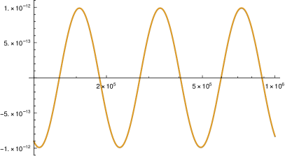
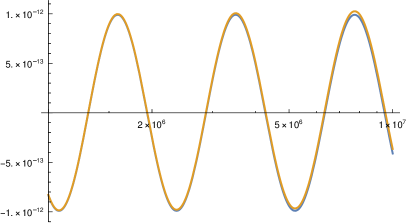
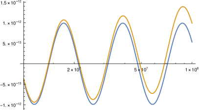
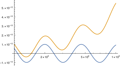
Figure 1: BURA (blue) and RS-BURA (yellow) errors $r_{\alpha,k}(z)-z^{-\alpha}$, respectively ${\widetilde{r}}_{\alpha,k,k^{\prime}}(z)-z^{-\alpha}$, $z\in(1,\delta^{-1}]$, $\alpha=0.25$, $k=85$, $k^{\prime}=46$, $\delta\in\{10^{-6},10^{-7},10^{-8},10^{-9}\}$.

The next numerical results illustrate the accuracy of RS-BURA. The test problem is defined by the following parameters: $\alpha=0.25$, $k=85$, $k^{\prime}=46$ and $\delta\in\{10^{-6},10^{-7},10^{-8},10^{-9}\}$. In accordance with Table 1, $E_{0.25,85}\approx 10^{-12}$. In Figure 1, the behavior of RS-BURA (yellow) and BURA (blue) approximations is compared. The RS-BURA error is always larger than the BURA error, as derived in (11). The largest differences are located at the right part of the interval. As expected, for fixed $(k,k^{\prime})$, the differences increase with the decrease of $\delta$. However, even in the worst case of $\delta=10^{-9}$, the accuracy ${\widetilde{E}}_{0.25,85,46}^{\delta}\approx 5\times 10^{-12}$. Indeed, according to (12) and Table 1, in this case the order of ${\widetilde{E}}_{\alpha,k,k^{\prime}}^{\delta}-E_{\alpha,k}$, thus the order of ${\widetilde{E}}_{\alpha,k,k^{\prime}}^{\delta}$ itself, should not exceed $9+(-5)-15=-11$. On the other hand, (12) implies that when $\delta>10^{-7}$ the order of ${\widetilde{E}}_{\alpha,k,k^{\prime}}^{\delta}-E_{\alpha,k}$ is lower than the order of $E_{\alpha,k}$, meaning that the sum reduction does not practically affect the accuracy. This is illustrated on the first row of Figure 1, where the plots of the two error functions are almost identical. This is a very promising result, taking into account that $\delta$ is controlled by the condition number of $\mathbb{A}$.

From a practical point of view, if $\Omega\subset{\mathbb{R}}^{3}$, and the FEM/FDM mesh is uniform or quasi uniform, the size of mesh parameter is limited by $h>10^{-4}$, corresponding to $N<10^{12}$. Such a restriction for $N$ holds true even for the nowadays supercomputers. Thus, we obtain that if $h\approx 10^{-4}$, the corresponding $\delta>10^{-9}$. In general, for real life applications, the FEM mesh is usually unstructured, including local refinement. This leads to some additional increase of the condition number of $\mathbb{A}$. However, the results in Figure 1 show that RS-BURA has a potential even for such applications.

The final conclusion of these tests is that some additional analysis is needed for better tuning of $k^{\prime}$ for given $k$, $\alpha$ and a certain targeted accuracy.

6 Concluding Remarks

The BURA method was introduced in [5], where the number of the auxiliary sparse SPD system solves was applied as a measure of computational efficiency. This approach is commonly accepted in [6, 7], following the unified view of the methods interpreted as rational approximations, where the degree $k$ is used in the comparative analysis.

At the same time, it was noticed that when iterative PCG solvers are used in BURA implementation even for relatively small degrees $k$, the number of iterations is significantly different, depending on the values of ${\widetilde{d}}_{i}$ (see [3] and the references therein).

The present paper opens a new discussion about the implementation of BURA methods in the case of larger degrees $k$. It was shown that due to the extremely large values of part of $|{\widetilde{d}}_{i}|$, the related auxiliary sparse SPD systems are very difficult (if possible at all) to solve. In this context, the first important question was whether BURA is even applicable to larger $k$ in practice. The proposed RS-BURA method shows one possible way to do this. The presented numerical tests give promising indication for the accuracy of the proposed reduced sum implementation of BURA.

The rigorous analysis of the new method (e.g., the proofs of (8), (11), and (12)) is beyond the scope of this paper.

Also, the results presented in Section 5 reopen the topic of computational complexity analysis, including the question of whether the almost optimal estimate $O((\log N)^{2}N)$ can be improved.

Acknowledgements

We acknowledge the provided access to the e-infrastructure and support of the Centre for Advanced Computing and Data Processing, with the financial support by the Grant No BG05M2OP001-1.001-0003, financed by the Science and Education for Smart Growth Operational Program (2014-2020) and co-financed by the European Union through the European structural and Investment funds.

The presented work is partially supported by the Bulgarian National Science Fund under grant No. DFNI-DN12/1.

References

- [1] Bonito, A., Pasciak, J.: Numerical approximation of fractional powers of elliptic operators. Mathematics of Computation 84(295), 2083–2110 (2015)
- [2] Software BRASIL, https://baryrat.readthedocs.io/en/latest/#baryrat.brasil
- [3] Harizanov, S., Kosturski, N., Margenov, S., Vutov, Y.: Neumann fractional diffusion problems: BURA solution methods and algorithms. Math Comp Simu. (2020), https://doi.org/10.1016/j.matcom.2020.07.018
- [4] Harizanov, S., Lazarov, R., Margenov, S.: A survey on numerical methods for spectral space-fractional diffusion problems. Frac Calc Appl Anal 23, 1605–1646 (2020)
- [5] Harizanov, S., Lazarov, R., Margenov, S., Marinov, P., Vutov, Y.: Optimal solvers for linear systems with fractional powers of sparse SPD matrices. Numer Linear Algebra Appl. 25(5), e2167 (2018), https://doi.org/10.1002/nla.2167
- [6] Harizanov, S., Lazarov, R., Margenov, S., Marinov, P., Pasciak, J.: Analysis of numerical methods for spectral fractional elliptic equations based on the best uniform rational approximation. Journal of Computational Physics 408, 109285 (2020), https://doi.org/10.1016/j.jcp.2020.109285
- [7] Hofreither, C.: A unified view of some numerical methods for fractional diffusion. Comp Math Appl. 80(2), 332–350 (2020)
- [8] Hofreither, C.: An algorithm for best rational approximation based on barycentric rational interpolation. Numer Alg (2021), https://doi.org/10.1007/s11075-020-01042-0
- [9] Stahl, H.: Best uniform rational approximation of on [0, 1]. Bull Amer Math Soc (NS) 28(1), 116–122 (1993)
- [10] Stahl, H.: Best uniform rational approximation of on [0, 1]. Acta Math 190(2), 241–306 (2003)
- [11] Varga, R.S., Carpenter, A.J.: Some numerical results on best uniform rational approximation of on . Num Alg 2(2), 171–185 (1992)